analyzes of solar chimney design - connecting repositories · the following should be considered in...
TRANSCRIPT

Master's ThesisJuly 2011Per Olaf Tjelflaat, EPT
Submission date:Supervisor:
Norwegian University of Science and TechnologyDepartment of Energy and Process Engineering
Analyzes of Solar Chimney Design
Elias Paez Ortega


Norwegian University Department of Energy
of Science and Technology and Process Engineering
NTNU
EPT-M-2011-
MASTER THESIS
for
Stud.techn. Elias Páez Ortega
Spring 2011
Analyzes of Solar Chimney Design
Analyse av design for solskorstein
Background and objective.
In the search for building installations that use less electricity to work, and where
noise generation is avoided, the solar chimney may be a good choice for buildings
with natural and hybrid ventilation.
The present study aims to investigate the basic principles of solar chimneys and to
test and improve the design of a solar chimney installed in the EPT lab.
The following should be considered in the project work:
1 A survey of solar chimney principles and of differences in design and
application.
2 An experimental assessment of the solar chimney installation in the EPT-lab.
3 CFD- simulation of a basic solar chimney design and of the solar chimney in the
EPT lab.
4 Comparison and discussion of results. Suggestions for improved solar chimney design.
-- ” --

Within 14 days of receiving the written text on the diploma thesis, the candidate
shall submit a research plan for his project to the department.
When the thesis is evaluated, emphasis is put on processing of the results, and that
they are presented in tabular and/or graphic form in a clear manner, and that they
are analyzed carefully.
The thesis should be formulated as a research report with summary both in English
and Norwegian, conclusion, literature references, table of contents etc. During the
preparation of the text, the candidate should make an effort to produce a well-
structured and easily readable report. In order to ease the evaluation of the thesis,
it is important that the cross-references are correct. In the making of the report,
strong emphasis should be placed on both a thorough discussion of the results and
an orderly presentation.
The candidate is requested to initiate and keep close contact with his/her academic
supervisor(s) throughout the working period. The candidate must follow the rules
and regulations of NTNU as well as passive directions given by the Department of
Energy and Process Engineering.
Pursuant to “Regulations concerning the supplementary provisions to the
technology study program/Master of Science” at NTNU §20, the Department
reserves the permission to utilize all the results and data for teaching and research
purposes as well as in future publications.
One – 1 complete original of the thesis shall be submitted to the authority that
handed out the set subject. (A short summary including the author’s name and the
title of the thesis should also be submitted, for use as reference in journals (max. 1
page with double spacing)).
Two – 2 – copies of the thesis shall be submitted to the Department. Upon
request, additional copies shall be submitted directly to research
advisors/companies. A CD-ROM (Word format or corresponding) containing the
thesis, and including the short summary, must also be submitted to the Department
of Energy and Process Engineering
Department of Energy and Process Engineering, 17. January 2011
__________________________ ________________________________
Olav Bolland Per Olaf Tjelflaat
Department Manager Academic Supervisor

Abstract The aim of this work to study the solar chimney installed in the EPT-lab of the
NTNU. The work starts with the development of a CFD model of the solar
chimney and comparing with the experimental data, showing a good accuracy of
the CFD results. The CFD model is used to compare three types of solar chimneys
for different heights and width; obtained that the chimney installed in the EPT-
lab gets higher flow rates in the most of the most of the cases. The CFD model
shows a uniform temperature and velocity inside the chimney that allows
developing a simple physical model of the chimney, which gives a good precision
of results. Finally a simplification of the solar chimney and other systems installed
in a building is simulated and also is developed another physical model for this
kind of building, giving an idea of the behavior of this solar house in diverse
conditions.

Contents Abstract .......................................................................................................... III
1 Introduction ........................................................................................... 1—1
2 Theory ................................................................................................... 2—2
2.1 Fluid dynamics ................................................................................ 2—2
2.1.1 Bernoulli equation................................................................... 2—3
2.1.2 Boundary layer ........................................................................ 2—5
2.1.3 Computational fluid dynamics ................................................. 2—7
2.2 Chimney ....................................................................................... 2—11
2.2.1 Solar Chimney ....................................................................... 2—12
3 Method................................................................................................ 3—16
3.1 Experimental results ..................................................................... 3—16
3.2 Development of CDF model .......................................................... 3—17
3.2.1 Boundary conditions ............................................................. 3—18
3.2.2 Chimney CFD model .............................................................. 3—25
3.2.3 Grid ....................................................................................... 3—28
3.2.4 Radiation model .................................................................... 3—29
3.2.5 Turbulence model ................................................................. 3—29
3.2.6 Results .................................................................................. 3—33
3.3 Simplification of the model ........................................................... 3—36
3.3.1 Setting .................................................................................. 3—36
3.4 Comparison different solar chimneys types .................................. 3—37
3.4.1 Results .................................................................................. 3—39
3.5 Performance of the solar chimney ................................................ 3—41
3.5.1 Theoretical equation ............................................................. 3—41
3.5.2 Validation of the theoretical equation ................................... 3—42
3.5.3 Pressure Vs Flow rate ............................................................ 3—45
3.5.4 Study of the control valve...................................................... 3—48
4 Behavior of a building with a solar chimney ......................................... 4—51
4.1 House model ................................................................................ 4—51
4.2 Effect of difference of temperatures ............................................. 4—52

4.3 Effect of the height of the chimney ............................................... 4—54
4.4 Effect of wind ............................................................................... 4—55
4.4.1 Wind velocity ........................................................................ 4—55
4.4.2 Pressure coefficient (Cp) ....................................................... 4—56
4.5 Effect of a heat recovery ............................................................... 4—57
5 Further work ........................................................................................ 5—61
6 Conclusion ........................................................................................... 6—62
7 References ........................................................................................... 7—63
Appendix 1 .................................................................................................. - 1 -
Pressure Loss Coefficients and Moody Diagram........................................ - 1 -
Appendix 2 .................................................................................................. - 4 -
Window data ........................................................................................... - 4 -
Appendix 3 .................................................................................................. - 5 -
Solar Chimney EPT-lab ............................................................................. - 5 -
Appendix 4 .................................................................................................. - 8 -
CFD Solar Chimney Model ........................................................................ - 8 -

Figures
Figur 2-1 Boundary layer on flat plane............................................................. 2—5
Figur 2-2 Turbulent boundary layer on flat plane ............................................ 2—5
Figur 2-3 Profile of a turbulent boundary layer ................................................ 2—6
Figur 2-4 Thermal boundary layer. Number of Prandtl .................................... 2—7
Figur 2-5 Chimney effect ............................................................................... 2—11
Figur 2-6 Solar chimney in the EPT-lab .......................................................... 2—13
Figur 2-7 Chimney type Tånga School ............................................................ 2—14
Figur 2-8 Standard solar chimney .................................................................. 2—15
Figur 3-1 Experimental results of velocity ...................................................... 3—16
Figur 3-2 Residuals configuration 1 ............................................................... 3—19
Figur 3-3 Temperatures configuration 1(K) .................................................... 3—20
Figur 3-4 Residuals configuration 2 ............................................................... 3—21
Figur 3-5 Residuals configuration 3 ............................................................... 3—21
Figur 3-6 Temperatures configuration 3 ........................................................ 3—22
Figur 3-7 Residuals configuration 4 ............................................................... 3—22
Figur 3-8 Residual configuration 5 ................................................................. 3—23
Figur 3-9 Temperatures configuration 5 ........................................................ 3—23
Figur 3-10 Residuals configuration 6 ............................................................. 3—24
Figur 3-11 Velocity configuration 6................................................................ 3—25
Figur 3-12 Stream function inlet .................................................................... 3—26
Figur 3-13 Chimney inlet ............................................................................... 3—26
Figur 3-14 Chimney CFD Model ..................................................................... 3—27
Figur 3-15 Grid fins ....................................................................................... 3—28
Figur 3-16 Grid wall ....................................................................................... 3—28
Figur 3-17 Fin temperature. Different radiation models ................................ 3—29
Figur 3-18 Velocity profile in the outlet (first simulation) .............................. 3—31
Figur 3-19 Profiles of turbulent dissipation rate ............................................ 3—31
Figur 3-20 Velocity profiles h=3m .................................................................. 3—32
Figur 3-21 Velocity profiles h=4,15m ............................................................. 3—33
Figur 3-22 velocity contours 3m and 4,15m ................................................... 3—34
Figur 3-23 Temperature contours 3m and 4,15m .......................................... 3—34
Figur 3-24 Temperatures profiles in chimney outlet ...................................... 3—35
Figur 3-25 Temperature contour of the collector .......................................... 3—35
Figur 3-26 Simplified model .......................................................................... 3—36
Figur 3-27 Models of the types of solar chimney ........................................... 3—38
Figur 3-28 Temperatures in type 3 ................................................................ 3—39
Figur 3-29 Mass flow Vs Width ...................................................................... 3—40
Figur 3-30 Mass flow Vs Height ..................................................................... 3—40
Figur 3-31 q Vs Q (H=cte) .............................................................................. 3—43

Figur 3-32 Temperature Vs Q (H=cte) ............................................................ 3—43
Figur 3-33 q Vs H (Q=cte) .............................................................................. 3—43
Figur 3-34 Temperature Vs H (Q=cte) ............................................................ 3—43
Figur 3-35 Efficiency (%) Vs Q ........................................................................ 3—44
Figur 3-36 Efficiency (%) Vs H ........................................................................ 3—44
Figur 3-37 Behavior of the control valve ........................................................ 3—46
Figur 3-38 Hydrostatic pressure from the chimney ........................................ 3—47
Figur 3-39 Pressure Vs Flow rate ................................................................... 3—47
Figur 3-40 Curves of different types of fan .................................................... 3—48
Figur 3-41 K Vs % opening ............................................................................. 3—49
Figur 3-42 % flow rate Vs % opening ............................................................. 3—50
Figur 3-43 Control valve flow characteristics ................................................. 3—50
Figur 3-44 Effect of authority in a linear valve ............................................... 3—50
Figur 4-1 House model .................................................................................. 4—51
Figur 4-2 Flow rate Vs difference of temperatures ........................................ 4—53
Figur 4-3 Flow rate Vs dT>0 ........................................................................... 4—54
Figur 4-4 Solar efficiency Vs difference of temperature ................................. 4—54
Figur 4-5 Flow rate vs. dT (various height) ..................................................... 4—55
Figur 4-6 Flow rate Vs dT (wind velocity) ....................................................... 4—56
Figur 4-7 rate Vs dT (Cp) ................................................................................ 4—57
Figur 4-8 Flow rate Vs dT (heat recovery) ...................................................... 4—58
Figur 4-9 solar efficiency Vs dT (heat recovery) ............................................. 4—59
Figur 4-10 Flow rate Vs dT>0 (heat recovery) ................................................ 4—59
Figur 4-11 Flow rate Vs dT (heat pipe recovery) ............................................ 4—60
Tables
Table 1 Experimental results .................................................................... 3—16
Table 2 Properties of the flow .................................................................. 3—17
Table 3 Comparison of velocity. Experimental Vs CFD .............................. 3—33
Table 4 Difference Coefficient of pressure drop ....................................... 3—37

Department of Energy
and Process engineering
Master thesis Spring 2011: Analyzes of Solar Chimney Design 1—1
1 Introduction The equipments, materials or human activity increase the pollutant
concentration inside the building, which affects to the indoor air quality.
Pollutant concentration can affect human health and productivity, which
makes necessary their removal. Traditionally the ventilation replaces the
indoor air for outdoor air, which has better quality.
The different modes of promoting air exchange are mechanical ventilation,
which allows controlling the flow rate all the moment, their quality and
temperature; and natural ventilation, which has less maintenance, makes
less noise and does not use electric energy to move the air.
The solar chimney is a system that uses the solar radiation to move the air,
improving the natural ventilation and in some cases providing fresh air for
the building. Many works were carried out the last two decades
demonstrating the advantages of solar chimney, for example the difference
of a traditional chimney and a solar chimney [1], the temperature impact of
a solar chimney [2] or their benefit in hybrid ventilation systems [3]. Other
works focus in the design of the solar chimney as the height, width or angle
of tilt, using in the most of the cases CFD tools to carry out the simulations
or experiments and developments physical and mathematical models for a
solar chimney [1, 4-7]. Also other works centers in the study of a building
with a solar chimney and other ventilation systems as a cooling cavity [8],
Trombe walls [9] or heat recovery [4]. All these studies shows the viability of
the this system and nowadays one can see that new buildings start to install
solar chimneys, like the Tånga School in Falkenberg Sweden [10].
The aim of this thesis is the new design of solar chimney made in the EPT-lab
of the Norwegian University of Science and Technology, which pretends to
demonstrate the advantages against others chimney’s design, develop a
physical model of the chimney and study the effect of a building with this
solar chimney.

Department of Energy
and Process engineering
Master thesis Spring 2011: Analyzes of Solar Chimney Design 2—2
2 Theory The aim of this chapter is to make an introduction of the theory, concepts
and principles used in this Thesis.
2.1 Fluid dynamics
The Navier-Stokes equations describe the motion of a fluid substance:
Continuity
𝜕𝜌
𝜕𝑡+ ∇ 𝜌𝑢 = 0
2.1
Momentum
𝜌𝜕𝑢
𝜕𝑡+ 𝜌𝑢 ∇ 𝑢 = −∇𝑝 +
𝜇
𝜌∇2𝑢 + 𝜌𝑓 𝑚 2.2
Energy
𝜌𝜕𝑐𝑝𝑇
𝜕𝑡+ 𝜌𝑢 ∇ 𝑐𝑝𝑇 = −𝑝∇𝑢 + 𝜏 :∇𝑢 + ∇ 𝑘∇𝑇 2.3
These equations do not have an analytic solution; therefore usually it used
simplification of these ones to achieve an approximate solution. The
dimensionless number is used to carry out these simplifications, as the
Reynolds number or the Rayleigh number.
The Reynolds number gives a measure of the ratio of inertial forces to
viscous forces and consequently quantifies the relative importance of these
two types of forces for given flow conditions.
𝑅𝑒 =𝜌𝑈𝐷
𝜇 2.4
When this number is high (Re>>1) the viscous forces can be neglected. Also
when Re<2300 in ducts a laminar flow occurs and for Re>4000 the flow is
turbulent.
The Rayleigh measures the importance of buoyancy driven flow). When the
Rayleigh number is below the critical value for that fluid, heat transfer is
primarily in the form of conduction; when it exceeds the critical value, heat
transfer is primarily in the form of convection.

Department of Energy
and Process engineering
Master thesis Spring 2011: Analyzes of Solar Chimney Design 2—3
𝑅𝑎 =𝑔𝛽∆𝑇𝑐𝑝𝜌
2𝐿3
𝜇𝑘 2.5
Besides, in a pure natural convection the Rayleigh number measures the
strength of the buoyancy-induced flow. When Ra<108 indicates an induced
laminar flow and a transition to turbulent flow among 108<Ra<1010.
2.1.1 Bernoulli equation
The Bernoulli equation is the result of thee simplification of the Navier-
Stokes equations assuming and inviscid fluid (Re>>1).
1
2𝜌𝑣2 + 𝑃𝑠 = 𝑐𝑡𝑒 = 𝑃𝑡 2.6
This means, if the velocity increases, the static pressure has to decrease.
This equation can be completed summing the effects of gravity and a turbo
machine.
1
2𝜌𝑣2 + 𝑃𝑠 + 𝜌𝑔 + ∆𝑃𝑓𝑎𝑛 = 𝑃𝑡 2.7
2.1.1.1 Pressure loss
In every duct system are present pressure losses due to the circulation of a
fluid inside a duct (primary pressure loss) and caused by additional
components as a valve, contractions or inlets (secondary pressure loss).
These pressure losses can be incorporated in the Bernoulli equation:
1
2𝜌𝑣2 + 𝑃𝑠 + 𝜌𝑔 + ∆𝑃𝑓𝑎𝑛 = 𝑃𝑡 +
1
2𝜌𝑣2 𝐾𝑑𝑟𝑜𝑝 2.8
The total coefficient of pressure drop ( 𝐾𝑑𝑟𝑜𝑝 ) is the sum of the primary
pressure loss and secondary pressure loss.
Primary pressure loss
𝑓 𝑅𝑒,𝜖
𝐷 2.9
𝐿
𝐷𝐿 = 𝑙𝑒𝑛𝑔 𝑜𝑓 𝑡𝑒 𝑑𝑢𝑐𝑡
𝐷 = 𝑦𝑑𝑟𝑎𝑢𝑙𝑖𝑐 𝑑𝑖𝑎𝑚𝑒𝑡𝑒𝑟 𝑜𝑓 𝑡𝑒 𝑑𝑢𝑐𝑡

Department of Energy
and Process engineering
Master thesis Spring 2011: Analyzes of Solar Chimney Design 2—4
𝑓 = 𝑓𝑟𝑖𝑐𝑡𝑖𝑜𝑛 𝑐𝑜𝑒𝑓𝑓𝑖𝑐𝑖𝑒𝑛𝑡 𝑜𝑓 𝐷𝑎𝑟𝑐𝑦
𝜖 = 𝑟𝑢𝑔𝑜𝑠𝑖𝑡𝑦 𝑜𝑓 𝑡𝑒 𝑑𝑢𝑐𝑡
The friction coefficient of Darcy can be estimated with the Moody
chart.
The secondary pressure loss depends of the components of the
system. Every component has its own coefficient of pressure loss,
and in the most of the cases can be calculated with charts. In this
thesis the secondary pressure are the inlet, outlet, nozzle and valve.
All this components have a constant coefficient of pressure loss.
All the charts used in this thesis can be found in Appendix 1
2.1.1.2 Buoyancy and stack effect
Buoyancy is the force, along with the gravity, involved in the movement to
upper positions of an object or fluid with less density than the fluid
surrounding.
In ideal gases when the temperature increases, the density decrease, thus a
movement between the cold and warm zones appears. This movement is
knowledge as Stack effect [11]. The pressure difference of the stack effect is
the next equation 2.10.
∆𝑃𝑠𝑡𝑎𝑐𝑘 = 𝑔𝐻∆𝜌
∆𝑃𝑠𝑡𝑎𝑐𝑘 = 𝜌𝑔𝐻∆𝑇
𝑇𝑖
2.10
The problem of this driven force is that it connects the energy and
momentum equations (equations 2.2 and 2.3) hindering the solution of the
problem.
To get a faster solution usually is used the Boussinesq Model. This model
treats the density as constant value in all the equations except in the
buoyancy term of the momentum equation.
𝜌 = 𝜌0 1 − 𝛽∆𝑇 → 𝛽∆𝑇 ≪ 1
2.11
∆𝑃𝑏𝑢𝑜𝑦𝑎𝑛𝑐𝑦 = 𝜌𝑔𝐻𝛽∆𝑇
2.12

Department of Energy
and Process engineering
Master thesis Spring 2011: Analyzes of Solar Chimney Design 2—5
2.1.2 Boundary layer
For flows with high Re, the effect of the viscosity is neglected, but areas
close to walls, the viscosity has to take into account because this area in the
most of the cases affect to the solution. This area is the boundary layer and
its study is very important to understand the behavior of the solar chimney
Figur 2-1 Boundary layer on flat plane
2.1.2.1 Turbulent boundary layer
As same happens in flows trough ducts, if the velocity or the length is
enough high (Re>>1), the boundary layer can change from laminar to
turbulent. In this case the layer is considerably more complex, at the same is
coarser, and dissipates more energy; thus the friction is higher. Nevertheless
the turbulent boundary layer moves the kinetic energy from the exterior to
the interior, improving the heat transfer between the flow and wall.
Figur 2-2 Turbulent boundary layer on flat plane

Department of Energy
and Process engineering
Master thesis Spring 2011: Analyzes of Solar Chimney Design 2—6
The turbulent boundary layer can be dived in two zones: the zone of defect
of velocities or outer law and zone near to the wall divided also in other two
zones, the viscous sublayer or inner law and the logarithmic sublayer or
overlap layer (Figur 2-3). This zone near the wall is very important to know
the mesh resolution in CFD simulations.
Figur 2-3 Profile of a turbulent boundary layer
2.1.2.2 Thermal boundary layer
In general, the temperature of the flow 𝑇∞ usually does not agree with the
temperature of the wall 𝑇𝑐 . As same as the velocity boundary layer, a
thermal boundary layer appears.
The study of the thermal boundary layer is important in the design of a solar
chimney since this is involved in the heat transfer between the wall and the
fluid and also in the stack effect.
The thickness of the thermal boundary layer depends of the number of
Prandtl, defined as:
𝑃𝑟 =𝑐𝑝𝜇
𝑘
2.13
𝑐𝑝 = 𝑆𝑝𝑒𝑐𝑖𝑓𝑖𝑐 𝑒𝑎𝑡
𝜇 = 𝑉𝑖𝑠𝑐𝑜𝑠𝑖𝑡𝑦
𝑘 = 𝑇𝑒𝑟𝑚𝑎𝑙 𝑐𝑜𝑛𝑑𝑢𝑐𝑡𝑖𝑣𝑖𝑡𝑦

Department of Energy
and Process engineering
Master thesis Spring 2011: Analyzes of Solar Chimney Design 2—7
When this number is higher than one (Pr>1) the thickness of the thermal
boundary layer is higher than the velocity boundary layer and the opposite if
Pr<1. When Pr is near to one, the sizes of both boundary layers have the
same order. Figur 2-4 shows this behavior.
Figur 2-4 Thermal boundary layer. Number of Prandtl
The thickness can be estimated with the following equation
𝛿𝑇𝐿
~ 𝑃𝑟−
12𝑅𝑒−
12 𝑃𝑟 < 1
𝑃𝑟− 13𝑅𝑒−
12 𝑃𝑟 > 1
2.14
𝛿𝑇 = 𝑇𝑖𝑐𝑘𝑛𝑒𝑠𝑠 𝑜𝑓 𝑡𝑒 𝑡𝑒𝑟𝑚𝑎𝑙 𝑏𝑜𝑢𝑛𝑑𝑎𝑟𝑦 𝑙𝑎𝑦𝑒𝑟
𝐿 = 𝐿𝑒𝑛𝑔 𝑜𝑓 𝑡𝑒 𝑤𝑎𝑙𝑙
2.1.3 Computational fluid dynamics
Computational fluid dynamics (CFD) is a computer based tool design to solve
a wide range of fluid mechanics problems. The CFD solves the three
equations of fluid flow (continuity, momentum and energy) approximately.
First the geometry of the model is discredited in thousand of cells and
nodes; the state of one node is affected by the neighboring nodes and the
boundary conditions.
The accuracy of the solution depends of many factors as the size of the cell,
the number of iterations, the boundary conditions selected, the size of the
domain, the models selected (turbulent, radiation or materials), the
discretization used (first order, second order,…) and other factors. Thus a
standard solution method does not exist and is necessary a deeply study of

Department of Energy
and Process engineering
Master thesis Spring 2011: Analyzes of Solar Chimney Design 2—8
the properties and conditions on each problem and in the mainly cases a
validation with experimental results.
In this Master Thesis it have been used Fluent to simulate the fluid flow,
since is one of the most development and used CFD programs.
2.1.3.1 RANS/ Turbulent models
When the Re>>1 the solution of the Navier-Stokes equations became
unstable with small perturbations. These perturbations develop as the flow
increases, leading to turbulence characterized for quick variation both
spatial and temporal. Since these fluctuations can be of small scale and high
frequency, they are too computationally expensive to simulate directly in the
most of engineering calculations.
In the most of the cases a time-averaged solution for the magnitudes is
enough. The equation of Reynolds Average Navier Stokes (RANS) is the result
of decomposing the flow magnitudes (velocity, pressure, temperature…) in
two, the average component and the fluctuating component.
𝑎 = 𝑎 + 𝑎′ 2.15
For example the momentum RANS equation is:
𝜌𝜕𝑢
𝜕𝑡+ 𝜌𝑢 ∇ 𝑢 = −∇𝑝 +
𝜇
𝜌∇2𝑢 +
1
𝜌∇(−𝜌𝑢′𝑢′ ) + 𝜌𝑓 𝑚 2.16
As one can see, the modified equation contain a new unknown variable,
−𝜌𝑢′𝑢′ , Reynolds stresses tensor represents the effects of turbulence and
must be modeled in order to close the equation. Thus turbulence models are
designed to determine this variable in terms of known quantities and close
the RANS equations.
−𝜌𝑢𝑖′𝑢𝑗
′ = 𝜇𝑡 𝜕𝑢𝑖𝜕𝑥𝑗
+𝜕𝑢𝑗
𝜕𝑥𝑖 −
2
3 𝜌𝑘 + 𝜇𝑡
𝜕𝑢𝑘𝜕𝑥𝑘
𝛿𝑖𝑗 2.17
Equation 2.17 represents the Boussinesq hypothesis what introduce the new
concept of turbulent viscosity 𝜇𝑡 (property of the flow). The concept of

Department of Energy
and Process engineering
Master thesis Spring 2011: Analyzes of Solar Chimney Design 2—9
turbulent viscosity reduces the computational cost. However it assumes 𝜇𝑡 is
an isotropic scalar quantity, which is not strictly true.
The alternative is to solve transport equations for each of the terms in the
Reynolds stress tensor, which means that five additional equations have to
be solved in 2D and seven in 3D.
Unfortunately, the choice of the turbulent model is not the same for all kinds
of problems. It is necessary to understand the capabilities and limitations of
the models, besides other considerations such as the accuracy, the
computational resources, time available and the class of problem. Fluent
provides a wide range of turbulence models, but only five are taken into
account in this Thesis.
Standard k-e model
It is a semi-empirical model based on model transport equation for
turbulent kinetic energy (k) and its dissipation rate (e).
𝜇𝑡 = 𝜌𝐶𝜇𝑘2
𝑒 2.18
𝐶𝜇 = 𝑐𝑜𝑛𝑠𝑡𝑎𝑛𝑡
The standard k-e model is the simplest “complete models” of
turbulence. It assumes that the flow is fully turbulent and the
molecular viscosity is negligible.
Realizable k-e problem
The realizable k-e model is an improvement of the standard k-e
problem. There are new formulations for the dissipation rate (e) and
for the turbulent viscosity.
𝐶𝜇 =1
𝐴𝑜 + 𝐴𝑠𝑈∗𝑘𝑒
2.19
𝐶𝜇 is no longer constant in this model.
The realizable k-e model predicts more accurately the spreading
rate of both planar and round jets. Also it can be used in transition
to turbulent flows.
Both models take into account the effect of the generation of k due
to buoyancy.

Department of Energy
and Process engineering
Master thesis Spring 2011: Analyzes of Solar Chimney Design 2—10
Transition k-kl-ω model
This model is used to predict boundary layer development and can
be used in flows with the transition of the boundary layer from
laminar to turbulent regime.
The disadvantage is that it resolves three transport equations
increasing the computational cost.
Transition SST model
It is a four transport equations model, which improves the accuracy
of simulations with flows in low free-stream turbulence
environments.
Reynolds stress model (RSM)
This is the most complete turbulent model that one can find in
Fluent. This model does not use the Boussinesq hypothesis, thus
five transport equations are solved in this model. Usually the model
gives more accurate results than the others in the mainly kind of
flows. This model requires closure assumptions employed in the
transport equations for the Reynolds stresses tensor.
2.1.3.2 Radiation models
In this section, it is going to describe the characteristic of the radiation
models and not the theory behind, due to its long formulation and
explanation.
Fluent provides five radiations models, but only are going to take into
account in the simulations of this Thesis.
The P-1 model is a diffusion equation, which is one of the radiations
who less computational resources use.
This model assumes gray radiation and that the all surfaces are
diffuse. It will be a loss of accuracy if the optical thickness is small
and also tends to over predict radiative fluxes from localized heat
sources.
The DO works with the entire range of optical thickness, with a
computational cost moderate.
The model allows to work with non gray radiation and also with
semi-transparent walls.

Department of Energy
and Process engineering
Master thesis Spring 2011: Analyzes of Solar Chimney Design 2—11
2.2 Chimney
A chimney is device usually used to remove the hot flue gas or smoke to the
atmosphere. It uses the stack effect to induce the movement.
In buildings, the chimney also is used in natural ventilation, taking
advantage of the differences of temperature between in-outside the
building.
Figur 2-5 Chimney effect
Adding equation 2.8 and 2.10 in the condition of Figur 2-5:
𝜌𝑔𝐻∆𝑇
𝑇𝑖=
1
2𝜌𝑣2 𝐾𝑑𝑟𝑜𝑝
𝑣 = 2𝑔𝐻
∆𝑇𝑇𝑖
𝐾𝑑𝑟𝑜𝑝→ 𝐶𝑑 =
1
𝐾𝑑𝑟𝑜𝑝
𝑞 = 𝐶𝑑 · 𝐴 2𝑔𝐻𝑇𝑖 − 𝑇𝑒𝑇𝑖
2.20
Equation 2.20 can be used to estimate the natural draught flow rate (q)
assuming that the heat loss negligible.

Department of Energy
and Process engineering
Master thesis Spring 2011: Analyzes of Solar Chimney Design 2—12
2.2.1 Solar Chimney
A solar chimney is a kind chimney that uses the solar radiation to increase
the temperature inside generating the stack effect to move the air. Usually it
is used as a way to improve the natural ventilation for a building. Also it can
be used to generate electrical energy, but in this cases the size it
considerably bigger, for example the solar tower built in Manzanares, Spain
was 195m high obtaining a maximum output power of 50 KW [12].
This Thesis is focus only in the solar chimney as a way to improve the natural
ventilation.
2.2.1.1 Chimney types
There is not only one design for solar chimney. It depends of the latitude of
the place, the height of the building, the solar collector or the materials.
Nowadays, the most widely used is that one that replaces part of the south
facade for a glazing allowing, the solar radiation, to get inside the chimney.
This Thesis studies three types of solar chimney.
Type 1
This solar chimney is installed in the EPT-lab for the Norwegian University of
Science and Technology. This chimney is the base of this Thesis, because is a
new type designed by this university in the project [13] and therefore not so
much information about the behavior and characteristics can be found.
In Figur 2-6 one can see the operating principle of this chimney. The solar
radiation passes through the glazing, situated in the down part of the south
façade, and it is absorbed by the solar collector (in the bottom of the
chimney). The solar collector is a high number of thin parallel metallic fins
(33 in the EPT-lab); the fin receives the solar radiation, increasing the
temperature of the surfaces, this generates a convection plume for each fin.
The distance between two consecutive fins is relative small (w=4,4cm) and
the angle from the centerline of the plume to the boundary is approximately
β=12.5º [14]. Thus the distance where two consecutives plumes touch each
other is:

Department of Energy
and Process engineering
Master thesis Spring 2011: Analyzes of Solar Chimney Design 2—13
=𝑤
2 · tan𝛽=
4,4
2 · tan 12,50
= 9,92𝑐𝑚 2.21
At this distance, one can consider a homogeneous temperature inside the
chimney. Note that the height of the chimney is bigger (300cm) than “h”,
therefore it is assumed that the height of the chimney and the height of the
stack effect it is the same.
Figur 2-6 Solar chimney in the EPT-lab
Type 2
This type of chimney is installed in the Tånga School in Falkenberg Sweden
[10]. It is designed for cold climates (higher latitudes)
Like the type 1, this chimney changes the down part of the south wall for a
glazing. The chimney is designed for cold climates (higher latitudes), that's
why just a part of the south facade is a glass to minimize the heat loss trough
the chimney, since this chimney also uses the stack effect of the building to
improve natural ventilation.

Department of Energy
and Process engineering
Master thesis Spring 2011: Analyzes of Solar Chimney Design 2—14
The radiation cross the window and it is absorbed by the solar collector, but
in this case it is the front wall, which is painted in black to improve the
absorption of radiation (Figur 2-7). In this case the height of the chimney and
the height of the stack there are not the same; as an approximation, the
begging of stack effect’s height can be calculated as the point where the
thermal boundary layer touches the south wall.
Figur 2-7 Chimney type Tånga School
Type3
This kind of solar chimney is the most used and studied [1, 4, 8, 9]; also it is
developed for warmer and tropical climates.
The design is very simple; the south wall is a glass allowing the radiation gets
to the solar collector, which is the front wall, also painted in black (Figur
2-8). Like the type 2, the height of the stack effect defers from the height of
the chimney; and can be calculated with the same conditions.

Department of Energy
and Process engineering
Master thesis Spring 2011: Analyzes of Solar Chimney Design 2—15
Figur 2-8 Standard solar chimney

Department of Energy
and Process engineering
Master thesis Spring 2011: Analyzes of Solar Chimney Design 3—16
3 Method
3.1 Experimental results
The basis of the development of the solar chimney’s CFD model is the
experimental results taken from the project “Development of Air solar
Collector” [13]. In this project can be found velocity, temperature,
height and radiation experimental data from the solar chimney studied in
this thesis.
As the CFD model will be a 2-D model, only is necessary take the midplane
data from the solar chimney. The results are showed in the next figure and
table.
Figur 3-1 Experimental results of velocity
Radiation (W/m^2) Velocity h=3m (m/s) Velocity h=4,15m (m/s)
881,7 0,35 0,506
846,4 0,362 0,524 Table 1 Experimental results
Also the temperature increase in the surroundings of the collector is around
ΔT≈2 and 3 K.
0,1
0,15
0,2
0,25
0,3
0,35
0,4
0,45
0,5
0,55
0,6
0 0,1 0,2 0,3 0,4 0,5
Vel
oci
ty (
m/s
)
Position (m)
881 W/m^2 h=3m
846 W/m^2 h=3m
881 W/m^2 h=4,15m
846 W/m^2 h=4,15m

Department of Energy
and Process engineering
Master thesis Spring 2011: Analyzes of Solar Chimney Design 3—17
3.2 Development of CDF model
The first step to build the CFD model is know the fluid field properties, as the
Reynolds number or Rayleigh number to select the turbulence, radiation and
fluid models
Properties of the flow:
Name Symbol Value
Density 𝜌 1,225𝑘𝑔
𝑚3
Viscosity 𝜇 1,7894 · 10−5𝑘𝑔
𝑚 · 𝑠
Specific heat 𝑐𝑝 1006,43𝐽
𝑘𝑔 · 𝐾
Thermal conductivity 𝑘 0,0242𝑊
𝑚 · 𝐾
Thermal expansion coefficient
𝛽 0,003411
𝐾
Hydraulic diameter 𝐷 0,5 𝑚
Longitude (height) 𝐿 3 𝑚
Average velocity 𝑈 0,4 𝑚
𝑠
Average difference of temperatures
∆𝑇 2 𝐾
Gravity 𝑔 9,81𝑚
𝑠2
Table 2 Properties of the flow
Reynolds number:
𝑅𝑒 =𝜌𝑈𝐷𝜇
= 13692 3.1
Rayleigh number:
𝑅𝑎 =𝑔𝛽∆𝑇𝑐𝑝𝜌
2𝐿3
𝜇𝑘= 6,3 · 109 3.2
Boussinesq fluid model:
𝛽∆𝑇 ≈ 0,07 ≪ 1 3.3

Department of Energy
and Process engineering
Master thesis Spring 2011: Analyzes of Solar Chimney Design 3—18
With these small differences of temperatures and the thermal
expansion coefficient, one can assume a Boussinesq model
In brief, it is working in a transition- turbulent problem, where is possible to
use the Boussinesq model for the buoyancy effects.
3.2.1 Boundary conditions
Have been studied six types of different configurations of boundary
conditions, to find which of these ones obtains a better converge of the
problem and less affect to the actual conditions.
In this case, has been used a simple model of a symmetric chimney, to
reduce the time of simulations. The six different types of configurations are
the following:
1. The limits of the model are walls with slip conditions and constant
temperature
2. There is a velocity inlet of 0.5 m down in the left wall, outflow of 0.1
m in the left at the top wall and the rest is a wall with slip conditions.
Both velocity inlet and wall have the same constant temperature.
3. The same as above, except that the velocity is in the top and the
outflow in the bottom.
4. The bottom is a velocity inlet, the top is an outflow condition and
the right side is a wall with slip conditions.
5. The same as above, except that the top is a pressure outlet
condition.
6. The bottom is a pressure inlet condition, the top a pressure outlet
and right side a wall with slip condition.
Where velocity inlet conditions are used has to be careful with the velocity
magnitude. In this cases have been used the ratio of Grashof and Reynolds
numbers:
𝐺𝑟
𝑅𝑒2=𝑔𝛽∆𝑇𝐿
𝑈2 3.4
This number measures the importance of buoyancy forces in a mixed
convection flow. When this number is bigger than unity, the buoyancy
effects are stronger than the velocity inlet. To be sure that the velocity inlet

Department of Energy
and Process engineering
Master thesis Spring 2011: Analyzes of Solar Chimney Design 3—19
does not interfere in the buoyancy forces of the problem, has been select a
ratio equal or bigger than 100, which corresponds a velocity of 0.01 m/s.
The model used in all the cases is the same and it is a symmetric chimney
with a radiator boundary condition in the bottom of this one with a heat flux
of 300 W/m2, the external temperature is 300 K (external walls and inlets)
and the turbulence model is standard k-e with standard wall functions and
thermal buoyancy effects.
Configuration 1 does not have problems with the convergence as it
shows in Figur 3-2, but take so many iterations to have a good value
of residuals (more than 6000 iterations to have residual of continuity
less than 10-4).
On the other hand, if one checks the temperature’s field in the
model, one can see that the temperature in the fluid increases
around 40C more than the external walls (Figur 3-3), therefore this
boundary condition does not satisfy the external temperature
condition.
Figur 3-2 Residuals configuration 1

Department of Energy
and Process engineering
Master thesis Spring 2011: Analyzes of Solar Chimney Design 3—20
Figur 3-3 Temperatures configuration 1(K)
The configuration 2 has an unstable solution as Figur 3-4 shows. The
reason of this is that the outlet condition is not long enough to take
all the heat of the radiator, then, the fluid in the model is warmer
than the inlet flow. This fact makes that the boundary conditions are
situated in the opposite direction of the natural flow, i.e. it has a
cold flow inlet in the bottom and the out flow on the top, so it is
forcing a cold flow goes up, when the normal is that the cold flow
goes down. This conclusion motivated the next boundary condition.

Department of Energy
and Process engineering
Master thesis Spring 2011: Analyzes of Solar Chimney Design 3—21
Figur 3-4 Residuals configuration 2
The configuration 3 has a better convergence than the 1 (Figur 3-5),
in less than 6000 iterations it has a residual continuity under 10-4.
Also, the configuration has the difference of temperatures between
external and the fluid problem, but in this case is lower (Figur 3-6),
around 20C.
Figur 3-5 Residuals configuration 3

Department of Energy
and Process engineering
Master thesis Spring 2011: Analyzes of Solar Chimney Design 3—22
Figur 3-6 Temperatures configuration 3
The configuration 4 is unstable (Figur 3-7), because in the outlet
appears a reflow induced for the chimney’s jet. The outlet condition
has problems with inverse flow; the solution is change to a pressure
outlet condition who can work with inverse flows, which it has been
done in the configuration 5.
Figur 3-7 Residuals configuration 4

Department of Energy
and Process engineering
Master thesis Spring 2011: Analyzes of Solar Chimney Design 3—23
Configuration 5 converges very well; as one can see in Figur 3-8
Residual configuration 5Figur 3-8 the residuals are very low after
6000 iterations, only the y-velocity and epsilon residuals are keep
the same value (around 10-3).
Figur 3-8 Residual configuration 5
The temperatures field (Figur 3-9) is what one might expect, i.e. the
inlet temperature is the same as the external and the only
differences of temperature appears inside the chimney and in the
jet.
Figur 3-9 Temperatures configuration 5

Department of Energy
and Process engineering
Master thesis Spring 2011: Analyzes of Solar Chimney Design 3—24
The Fluent’s manual suggests use this configuration in buoyancy
effect problems [15]. The value of gauge total pressure was taken
following the advice of Fluent’s manual.
Figur 3-10 Residuals configuration 6
This configuration is which one gives the best results of
convergence. In 2250 iterations, all the residuals are below 10-5,
which is taken into account as the value of convergence. The
temperatures field is the same as the configuration 6.
The problem of this configuration is the velocity, as one can see in
Figur 3-11, the inlet velocity is constant in the whole pressure inlet
boundary condition and also the magnitude is close to the velocity
inside the chimney. That means, that the influence of the radiation
in the value of the flow rate will be minimized due to that the
velocity in the inlet boundary condition is around 20% the velocity
inside the chimney.

Department of Energy
and Process engineering
Master thesis Spring 2011: Analyzes of Solar Chimney Design 3—25
Figur 3-11 Velocity configuration 6
Finally the configuration 5 has been selected due to it is which gives the best
relation between convergence and approximation to the real problem in the
results (velocity and temperature).
3.2.2 Chimney CFD model
Before making the full model of the chimney, different inlets have been
simulated. This action has been made to avoid the recirculation flow that
appears in the inlet.
First, the solar collector had been replaced for a radiator boundary
condition, fixing the heat flow, to study the flow around the chimney
In the first case (without inlet), one can see the recirculation flow at the
inlet, that is the reason why different inlets configurations have been tested
to try to avoid this reflow. In any case, these configurations do not affect to
the stack effect, as this ones are always before the collector.
The reason, to find an inlet for the chimney, is that this one will join to a
ventilation duct and this reflow hardly appears. Other reasons are the
stability of the simulation and the energy balance in the chimney (some of
the heat goes out and affect to the stack effect).
The following pictures show the steps to achieve the inlet for the chimney

Department of Energy
and Process engineering
Master thesis Spring 2011: Analyzes of Solar Chimney Design 3—26
Figur 3-12 Stream function inlet
Finally, it has been selected the next inlet.
Figur 3-13 Chimney inlet
The selected model to simulate the chimney has:
The boundary conditions selected before.
The inlet selected, without slip conditions.
The outside of the chimney is completely different of the inside; the
reason is to avoid the reflow what appears on the outside of the
inlet.
The solar collector has been changed for 32 fins. One side of the fin
will generated a heat flow, simulating the incident radiation; the
other side will be adiabatic.
The inside (wall and glazing) of the chimney has been considered
completely insulated. This approximation can be prove easily:

Department of Energy
and Process engineering
Master thesis Spring 2011: Analyzes of Solar Chimney Design 3—27
The U-Value for the glazing is 1.2 W/m2, the difference of
temperature is around 2K and the area of glazing is 0.75m2/m, so
the heat loss will be:
𝑄 = 𝑈 ∗ 𝐴 ∗ 𝛥𝑇 = 1,2 ∗ 0,75 ∗ 2 = 1,776𝑊/𝑚
Usually the input power is around 500W/m, which means
that the heat loss is less than 1%.
The heat flow generated in the fins has been estimated
with the next equation:
𝑄 = 𝐼 ∙ cos𝛼 ∙ 𝛿 ∙𝑤
tan𝛼 3.5
𝐼 = 𝑅𝑎𝑑𝑖𝑎𝑡𝑖𝑜𝑛 𝑊
𝑚2
𝛼 = 𝑎𝑛𝑔𝑙𝑒 𝑏𝑒𝑡𝑤𝑒𝑒𝑛 𝑡𝑒 𝑖𝑛𝑐𝑖𝑑𝑒𝑛𝑡 𝑟𝑎𝑑𝑖𝑎𝑡𝑖𝑜𝑛 𝑎𝑛𝑑 𝑡𝑒 𝑜𝑟𝑖𝑧𝑜𝑛𝑡𝑎𝑙 𝑝𝑙𝑎𝑛𝑒
𝛿 = 𝑡𝑟𝑎𝑛𝑠𝑚𝑖𝑡𝑎𝑛𝑐𝑒 𝑜𝑓 𝑡𝑒 𝑤𝑖𝑛𝑑𝑜𝑤
The factor 𝑤
tan𝛼 is the part of the fin which receives the bean radiation
(Appendix 2 and Appendix 3).
Figur 3-14 Chimney CFD Model

Department of Energy
and Process engineering
Master thesis Spring 2011: Analyzes of Solar Chimney Design 3—28
3.2.3 Grid
The grid selected has particular care with the velocity and thermal boundary
layers in the wall inside the chimney and in the fins of the collector, as one
can see in the next pictures.
Figur 3-15 Grid fins
Figur 3-16 Grid wall
Department of Energy
and Process engineering
Master thesis Spring 2011: Analyzes of Solar Chimney Design 3—29
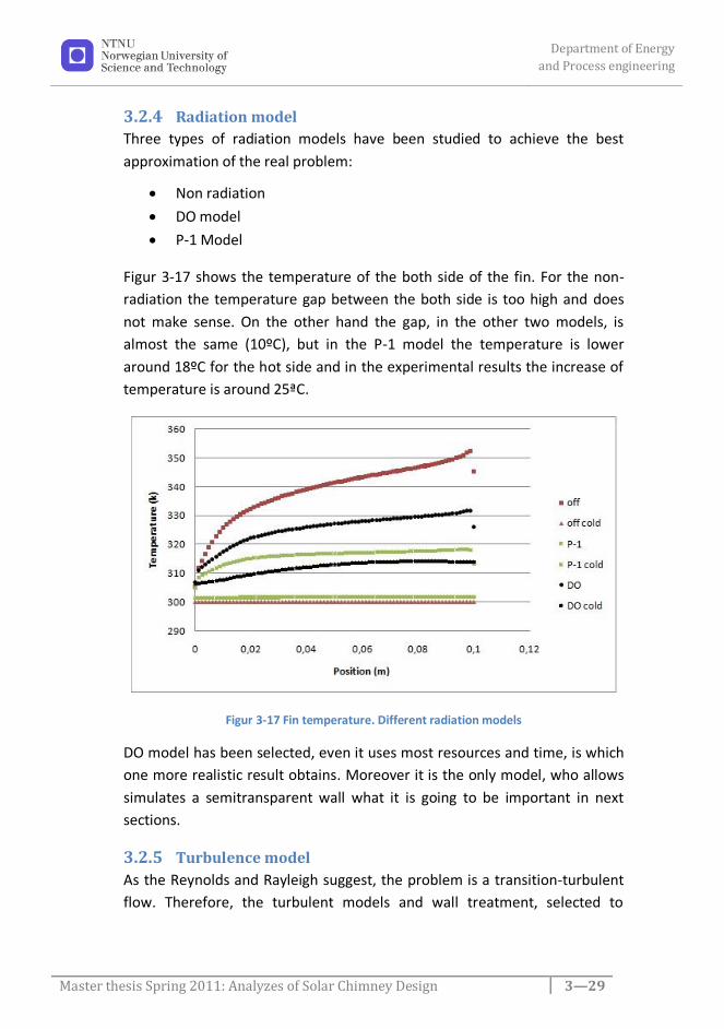
3.2.4 Radiation model
Three types of radiation models have been studied to achieve the best
approximation of the real problem:
Non radiation
DO model
P-1 Model
Figur 3-17 shows the temperature of the both side of the fin. For the non-
radiation the temperature gap between the both side is too high and does
not make sense. On the other hand the gap, in the other two models, is
almost the same (10ºC), but in the P-1 model the temperature is lower
around 18ºC for the hot side and in the experimental results the increase of
temperature is around 25ªC.
Figur 3-17 Fin temperature. Different radiation models
DO model has been selected, even it uses most resources and time, is which
one more realistic result obtains. Moreover it is the only model, who allows
simulates a semitransparent wall what it is going to be important in next
sections.
3.2.5 Turbulence model
As the Reynolds and Rayleigh suggest, the problem is a transition-turbulent
flow. Therefore, the turbulent models and wall treatment, selected to

Department of Energy
and Process engineering
Master thesis Spring 2011: Analyzes of Solar Chimney Design 3—30
compare with the experimental results, have been taken in account this
assumption.
Four models of turbulence had been tested; k-e model, Transition k-kl-w
model, Transition SST model and Reynolds stress model.
In the k-e model, the lash of full buoyancy effect and thermal effect were
ticked due to the flow across the chimney is leaded of these effects. Two
near wall treatment has been simulated; the Standard wall function and the
Enhanced wall treatment. Also two k-e models were taken in account; the
Standard model and the Realizable model.
3.2.5.1 Setting values
The difference of the velocity at the outlet of the chimney is insignificant,
when the radiation varies between 881.7 W/m2 and 846.4 W/m2, as the
experimental data shows. Therefore, the average of these two radiations
(864.05 W/m2) has been selected as an incident radiation of the CFD
simulations. Then the heat flux generated on the fins is:
𝑄 = 𝐼 ∙ cos𝛼 ∙ 𝛿 ∙𝑤
tan𝛼
𝑄 = 864,05 ∙ cos 330 ∙ 0,63 ∙0,044
0,07tan 330 = 186,35 𝑊/𝑚2
3.6
3.2.5.2 First simulation
In the first simulations, the turbulence values of the boundary conditions (k
and e) and the turbulent model constants are the default.
In this case the transition SST model (4 equations) and the Reynolds stress
model (5 equations) had problems with the convergence, so these models
were discarded for next simulations.
Figur 3-18 shows the velocity profiles in the outlet velocity for the
turbulence models and the experimental results of a 3 m high chimney. In all
the cases the velocity is almost the double of the experimental. Before
changed the values of the turbulent model constants and boundary
condition, some model has been removed:

Department of Energy
and Process engineering
Master thesis Spring 2011: Analyzes of Solar Chimney Design 3—31
The Transition k-kl-w model has removed because the velocity
profile is uniform and the experimental results shows that closed to
the wall the velocity is higher than in the center.
The k-e model with Standard wall functions owing to the opposite,
the difference of velocities is too higher compare to the
experimental results.
Figur 3-18 Velocity profile in the outlet (first simulation)
It had been compared the graphics of turbulence properties of the flow, to
know what changes have to make in the turbulence models. Figur 3-19
shows the contours of turbulent dissipation rate (e) and the mistake of the
model, as one can see the value of e is too high in the pressure outlet and
velocity inlet boundaries conditions.
Figur 3-19 Profiles of turbulent dissipation rate
0,25
0,3
0,35
0,4
0,45
0,5
0,55
0,6
0,65
0,7
0,025 0,125 0,225 0,325 0,425
velo
city
(m
/s)
Possition (m)
3 eq
2eq_stn_std
2eq_stn_enh
2eq_real_std
2eq_real_enh
846 W/m^2
881 W/m^2

Department of Energy
and Process engineering
Master thesis Spring 2011: Analyzes of Solar Chimney Design 3—32
3.2.5.3 Second simulation
Changing the turbulent dissipation rate (e) to 0.3 in the velocity inlet and
pressure outlet boundary conditions, the CFD results agree with the
experimental as it is shows in Figur 3-20. The difference between the
Standard k-e model and Realizable k-e model is that the velocity in the last
one is a little bit lower.
Figur 3-20 Velocity profiles h=3m
For height of the chimney of 4.15m (Figur 3-21) the velocity profiles of
experimental and CFD simulations are also similar.
To select the turbulence model, it has been compared the average velocity
of the experimental results and the CFD simulation for both heights (Table
3). For 3m the two turbulent models are inside the limits forced for the
experimental velocities, but for 4.15m the Standard k-e is upper this limits.
Therefore the Realizable k-e model with Enhanced wall function was chosen
to simulate the solar chimney.
0,1
0,15
0,2
0,25
0,3
0,35
0,4
0,45
0,025 0,125 0,225 0,325 0,425
velo
city
(m
/s)
Position (m)
881 W/m^2
846 W/m^2
2eq_real_enh
2eq_stn_enh

Department of Energy
and Process engineering
Master thesis Spring 2011: Analyzes of Solar Chimney Design 3—33
Figur 3-21 Velocity profiles h=4,15m
Radiation (W/m^2) Velocity h=3m (m/s) Velocity h=4,15m (m/s)
881,7 0,350 0,506
846,4 0,362 0,524
2eq_real_enh 0,350 0,515
2eq_stn_enh 0,361 0,539 Table 3 Comparison of velocity. Experimental Vs CFD
3.2.6 Results
As a summary the CFD model selected to simulate the solar chimney and
which one gives the more realistic results is:
The boundary conditions are a velocity inlet in the bottom of 0.01
m/s with a inlet temperature of 300 K, the inlet turbulent kinetic
energy of 1 m2/s2 and a turbulent dissipation rate of 0.3 m2/s3; the
right and the left side is a wall with slip condition and a temperature
of 300 K; and the top is a pressure outlet with the same backflow
conditions as the velocity inlet. Appendix 4
A smooth chimney inlet to avoid the recirculation.
The radiation model is DO model with 4 theta and pi divisions, 4
theta and pi pixels and 10 flow iterations per radiation iteration.
The Realizable k-e model with Enhanced wall function.
0,15
0,25
0,35
0,45
0,55
0,65
0,025 0,125 0,225 0,325 0,425
velo
city
(m
/s)
Position (m)
881 W/m^2
846 W/m^2
2eq_real_enh
2eq_stn_enh

Department of Energy
and Process engineering
Master thesis Spring 2011: Analyzes of Solar Chimney Design 3—34
Figur 3-22 velocity contours 3m and 4,15m
Figur 3-23 Temperature contours 3m and 4,15m

Department of Energy
and Process engineering
Master thesis Spring 2011: Analyzes of Solar Chimney Design 3—35
Figur 3-24 Temperatures profiles in chimney outlet
The before figures show an interesting conclusions
The flow across the model can be considered as a symmetric (Figur
3-22)
The temperature is almost constant inside the chimney (Figur 3-23,
Figur 3-24 and Figur 3-25)
The whole height of the chimney is taking into account in the stack
effect. This is the main difference on the other types of solar
chimneys.
Figur 3-25 Temperature contour of the collector
300
300,5
301
301,5
302
302,5
303
303,5
304
304,5
305
-0,25 -0,15 -0,05 0,05 0,15 0,25
Tem
pe
ratu
re (
k)
position (m)
3 m
4,15m

Department of Energy
and Process engineering
Master thesis Spring 2011: Analyzes of Solar Chimney Design 3—36
3.3 Simplification of the model
As one can see on the before results, the flow inside the chimney can be
consider as symmetric and with constant temperature. This fact suggests
change the model to a symmetric one with a coarse grid to future
simulations of the chimney.
The proposed model has the same turbulent model, radiation model,
boundary conditions (except for the symmetry) and the inlet. On the other
hand, the chimney’s width is constant and equal to the outside of the
chimney (0.5 m); the solar collector has been replaced to a radiator
boundary condition; and the use of the radiation model will be study.
Figur 3-26 Simplified model
3.3.1 Setting
The model has to have the same power as the real one, which means that
the heat flux in the radiator and the collector is not the same. The ratio
between the heat fluxes is the next:
𝑃 = 𝐼𝑟𝑒𝑎𝑙 ∙ 𝐴𝑐𝑜𝑙𝑙𝑒𝑐𝑡𝑜𝑟 = 𝐼𝑟𝑎𝑑𝑖𝑎𝑡𝑜𝑟 ∙ 𝐴𝑟𝑎𝑑𝑖𝑎𝑡𝑜𝑟
𝐼𝑟𝑎𝑑𝑖𝑎𝑡𝑜𝑟 = 𝐼𝑟𝑒𝑎𝑙𝐴𝐶𝑜𝑙𝑙𝑒𝑐𝑡𝑜𝑟𝐴𝑟𝑎𝑑𝑖𝑎𝑡𝑜𝑟
= 𝐼𝑟𝑒𝑎𝑙𝑛𝑢𝑚𝑏𝑒𝑟 𝑜𝑓 𝑓𝑖𝑛𝑠 ∙ 𝑓𝑖𝑛
𝐴𝑟𝑎𝑑𝑖𝑎𝑡𝑜𝑟
𝐼𝑟𝑎𝑑𝑖𝑎𝑡𝑜𝑟 = 𝐼𝑟𝑒𝑎𝑙33 ∙ 0,07𝑚2
0.5𝑚2

Department of Energy
and Process engineering
Master thesis Spring 2011: Analyzes of Solar Chimney Design 3—37
𝐼𝑟𝑎𝑑𝑖𝑎𝑡𝑜𝑟 = 4,62 ∙ 𝐼𝑟𝑒𝑎𝑙 3.7
If there is not any setting in the model (except for the heat flux), it is easy to
check that the flow rate and the temperature will be higher. Therefore is
necessary to introduce a pressure drop in the radiator.
Following the advices of Fluent’s Manual [15], it has been calculated the
difference of the coefficient of pressure drop between the real and the
simplification model for three heat powers in the radiator. Table 4 shows
that the difference is approximately constant, and one can assume that the
pressure drop across the radiator is the average of this values, what is K=0.5
Q (W) Difference K
150 0,467630484
450 0,528222212
960 0,498409162 Table 4 Difference Coefficient of pressure drop
Also, this value can be calculated easily, assuming the difference of pressure
drops, between the real and the simple model, is the reduction between the
inlet and the outlet. The pressure drop coefficient of a nozzle is usually
constant and can be estimate in tables; in this case the value is around
K=0.48.
3.4 Comparison different solar chimneys types
The two models studied in this section has the same geometry, also the
same boundary condition, turbulent and radiation models and the same
assumption of the solar radiation can be estimated as a heat flux in the wall.
The solar radiation (𝐼𝑠𝑢𝑛 ) is the same in all the models to compare the
difference of these three solar chimneys

Department of Energy
and Process engineering
Master thesis Spring 2011: Analyzes of Solar Chimney Design 3—38
Figur 3-27 Models of the types of solar chimney
Type 1
This model is the simplification of the solar chimney in the EPT-lab.
The heat flux in the radiator has the following equation
𝑄 = 𝐼𝑠𝑢𝑛 ∙ 4,62 ∙ cos𝛼 ∙ 𝛿 ∙𝑤
tan𝛼 3.8
Type 2
This is the model of the Swedish school. The solar collector
(absorption wall) has always the same height (0,5 m) and the heat
flux generated is:
𝑄 = 𝐼𝑠𝑢𝑛 ∙ cos𝛼 ∙ 𝛿 3.9
As the equal as the model type 1, it has been assumed that the walls
of the chimney are completely insulated and there is no appreciable
effect of the window in the solution of the simulation.
Type 3
This is the standard solar chimney for mild climates, the southern
wall is a glazing and the interior northern wall is the solar collector.
In this case, the assumption of insulated wall is not possible in the

Department of Energy
and Process engineering
Master thesis Spring 2011: Analyzes of Solar Chimney Design 3—39
glazing. Therefore, a new boundary condition for the glazing had
developed:
The characteristic of the glazing (Appendix 2) shows that a
percentage of the solar energy is transmitted (63%), other is
reflected (23%) and other is absorbed (14%). This absorbed radiation
is simulated as a heat generation rate (W/m3) inside the window:
𝑄𝑔𝑙𝑎𝑧𝑖𝑛𝑔 =𝛾 ∙ 𝐼𝑠𝑢𝑛 ∙ cos 𝛼
𝑒
3.10
𝛾 = 𝑝𝑒𝑟𝑐𝑒𝑛𝑡𝑎𝑔𝑒 𝑜𝑓 𝑠𝑜𝑙𝑎𝑟 𝑎𝑏𝑠𝑜𝑟𝑡𝑖𝑜𝑛
𝑒 = 𝑡𝑖𝑘𝑛𝑒𝑠𝑠 𝑜𝑓 𝑡𝑒 𝑔𝑙𝑎𝑧𝑖𝑛𝑔
Furthermore, the glazing properties (density, conductivity,
absorption coefficient, cp) has been put in the boundary conditions
of the southern wall.
The heat flux in the solar collector is the same as the type 2,
equation 3.9
3.4.1 Results
The results of the temperature in the solar collector and the glazing have
been compared with the simulations carried out in other work [7], that show
an increment around 30ºC in the solar collector and 12ºC in the glazing,
which is similar to the results simulated, 28ºC and 13ªC correspondingly (see
Figur 3-28).
Figur 3-28 Temperatures in type 3
Department of Energy
and Process engineering
Master thesis Spring 2011: Analyzes of Solar Chimney Design 3—40
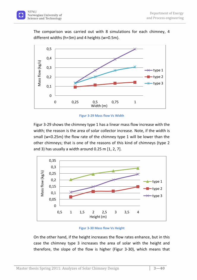
The comparison was carried out with 8 simulations for each chimney, 4
different widths (h=3m) and 4 heights (w=0.5m).
Figur 3-29 Mass flow Vs Width
Figur 3-29 shows the chimney type 1 has a linear mass flow increase with the
width; the reason is the area of solar collector increase. Note, if the width is
small (w<0.25m) the flow rate of the chimney type 1 will be lower than the
other chimneys; that is one of the reasons of this kind of chimneys (type 2
and 3) has usually a width around 0.25 m [1, 2, 7].
Figur 3-30 Mass flow Vs Height
On the other hand, if the height increases the flow rates enhance, but in this
case the chimney type 3 increases the area of solar with the height and
therefore, the slope of the flow is higher (Figur 3-30), which means that
0
0,1
0,2
0,3
0,4
0,5
0 0,25 0,5 0,75 1
Mas
s fl
ow
(kg/
s)
Width (m)
type 1
type 2
type 3
0
0,05
0,1
0,15
0,2
0,25
0,3
0,35
0,5 1 1,5 2 2,5 3 3,5 4
Mas
s fl
ow
(kg/
s)
Height (m)
type 1
type 2
type 3

Department of Energy
and Process engineering
Master thesis Spring 2011: Analyzes of Solar Chimney Design 3—41
chimney type 3 gets higher flow when the height of the chimney is enough
high, in this case around 5 m. Note that, the slop changes between 2 m and
3 m in the chimneys type 2 and 3, the reason is the link of the two thermal
layers (southern and northern walls).
3.5 Performance of the solar chimney
3.5.1 Theoretical equation
Taking into account a uniform velocity and temperature inside the chimney,
as it was demonstrated in 3.2.6, the theoretical flow rate will be:
Energy balance in the chimney
𝑄 = 𝑞𝜌𝑐𝑝 𝑇𝑜𝑢𝑡 − 𝑇𝑒𝑥𝑡
𝑇𝑜𝑢𝑡 = 𝑇𝑒𝑥𝑡 +𝑄
𝑞𝜌𝑐𝑝
3.11
Approximation velocity profile constant
𝑉 ∙ 𝐴 = 𝑞 3.12
Drag coefficient Vs constant pressure loss
𝐶𝑑 =1
𝐾𝑙𝑜𝑠𝑠 3.13
Bernoulli equation
𝜌𝑔𝐻 𝑇𝑜𝑢𝑡 − 𝑇𝑒𝑥𝑡
𝑇𝑒𝑥𝑡=
1
2𝜌𝑉2 𝐾𝑙𝑜𝑠𝑠
𝜌𝑔𝐻 𝑇𝑜𝑢𝑡 − 𝑇𝑒𝑥𝑡 =1
2𝜌𝑇𝑜𝑢𝑡
𝑞
𝐴𝐶𝑑
2
𝑞3 + 𝑞2𝑄
𝑇𝑒𝑥𝑡 𝜌𝑐𝑝− 𝐴𝐶𝑑 22𝑔𝐻𝑄
𝑇𝑒𝑥𝑡 𝜌𝑐𝑝= 0
3.14

Department of Energy
and Process engineering
Master thesis Spring 2011: Analyzes of Solar Chimney Design 3—42
The value of Cd can be calculated as a function of the sum of coefficient of
pressure loss of the inlet, the nozzle, the outlet and the friction of the walls
𝐾 = 𝐾𝑖𝑛𝑙𝑒𝑡 + 𝐾𝑛𝑜𝑧𝑧 + 𝐾𝑜𝑢𝑡𝑙𝑒𝑡 + 𝑓𝐻
𝐷 3.15
In the Appendix 1, one can find the values of this coefficient depending the
geometry
In theory, Cd is function of the flow rate, because the factor f depends of the
number of Re, but 𝑓 ∈ 0.04 , 0.015 which gives a 𝐶𝑑 ∈ 0.75 ,0.788 , who
is not a big difference. Therefore one can consider the Cd as function only of
the height:
𝐾 = 0.04 + 0.48 + 1 + 0.04𝐻
0.5
𝐶𝑑 =1
1.52 + 0.08𝐻
3.16
The solution of equation 3.14 is longer to show, but the method to resolve a
third degree equation can be found in [13]
3.5.2 Validation of the theoretical equation
To valid the equation 3.14, 9 simulations have calculated; 5 for diverse values
of Q (100 W to 300W) and 4 for diverse values of height (1m to 4m). The
reference value of Q is 300 W, of H is 3m, except the cases when varies one
of this values.

Department of Energy
and Process engineering
Master thesis Spring 2011: Analyzes of Solar Chimney Design 3—43
3.5.2.1 Flow rate as a function of radiation
Figur 3-31 q Vs Q (H=cte)
Figur 3-32 Temperature Vs Q (H=cte)
3.5.2.2 Flow rate as a function of height
Figur 3-33 q Vs H (Q=cte)
Figur 3-34 Temperature Vs H (Q=cte)
As one can see in the results, the theoretical equation estimates with
precision the values of flow rate and temperature in the chimney.
The kinetic energy efficiency is one of the solar chimney properties allows
compare with other technologies. This efficiency can be calculated as the
coefficient between the kinetic energy and the power generated in the solar
collector:
0
0,05
0,1
0,15
0,2
0,25
0 100 200 300 400
q(m
3/s
)
Q(W)
q CFD
q theoretical
300,3
300,6
300,9
301,2
301,5
0 100 200 300 400
T(K
)
Q(W)
Temp CFD
Temp theoretical
0,08
0,1
0,12
0,14
0,16
0,18
0 1 2 3 4 5
q(m
3/s
)
h(m)
q CFD
q theoretical 300,6
300,7
300,8
300,9
301
301,1
301,2
0 1 2 3 4 5
T(K
)
h(m)
Temp CFD
Temp theoretical

Department of Energy
and Process engineering
Master thesis Spring 2011: Analyzes of Solar Chimney Design 3—44
𝜂 =
12𝑚 𝑉2
𝑄=
12𝑞𝜌
𝑞𝐴
2
𝑄
𝜂 =𝑞3𝜌
2𝑄𝐴2
3.17
Figur 3-35 Efficiency (%) Vs Q
Figur 3-36 Efficiency (%) Vs H
Figur 3-35 and Figur 3-36 show that if one wants to improve the efficiency of
the solar chimney, he has to increase the height of the chimney and not the
area of the solar collector (more heat generation).
Another important conclusion of both figures is that the efficiency is
constant with the radiation (Q) and increase linearly with the height, which
means:
𝑞 = 𝜂2𝑄𝐴2
𝜌
3 𝑎𝑛𝑑 𝑞 =
𝑐𝑡𝑒𝐻2𝑄𝐴2
𝜌
3
0,002
0,003
0,004
0,005
0,006
0,007
0,008
0,009
0,01
0 2000 4000 6000 8000 10000 12000
Q (W)
efficien…
0
0,005
0,01
0,015
0,02
0,025
0,03
0,035
0 2 4 6 8 10 12
H (m)
effic…

Department of Energy
and Process engineering
Master thesis Spring 2011: Analyzes of Solar Chimney Design 3—45
The value of this constant or η can be calculated if the Boussinesq
approximation is supposed for a gas
∆𝑇
𝑇= 𝛽∆𝑇 3.18
Thus the new equation for the flow rate will be:
𝑔𝐻𝛽 𝑇𝑜𝑢𝑡 − 𝑇𝑒𝑥𝑡 =1
2 𝑞
𝐴𝐶𝑑
2
𝜌𝐻𝛽𝑄
𝑞𝜌𝑐𝑝=
1
2 𝑞
𝐴𝐶𝑑
2
𝑞 = 𝐴𝐶𝑑 22𝑔𝐻𝛽𝑄
𝜌𝑐𝑝
3
3.19
Also, this demonstrates, as a good election, the supposition of Boussinesq
for the CFD simulations.
3.5.3 Pressure Vs Flow rate
The function Pressure Drop Vs Flow rate serves to know the behavior of the
chimney for different pressures loss and also to compare with fans, since the
cross between these curves (system and fan) marks the operations point.
A simple control valve was designed to simulate diverse conditions of work,
this valve consist in two plates, situated in the outlet, are closing form the
outside in (see Figur 3-37).

Department of Energy
and Process engineering
Master thesis Spring 2011: Analyzes of Solar Chimney Design 3—46
Figur 3-37 Behavior of the control valve
Six simulations were carried out for diverse openings of the valve, from fully
open to 10% of aperture. Less percentage of opening makes the simulation
unstable and also the assumptions of adiabatic wall does not satisfy because
the increase of the air temperature.
To calculate the pressure drop across the chimney, it has been taken the
pressure data from 3 lines: one is the symmetric line, other pass close to the
wall (0.05m from the wall) and the other is parallel to these ones and
outside from the chimney.
The outside line severs to calculated the hydrostatic pressure (equation
3.20), since Fluent uses a reduction constant (A) for the simulations. Once
the hydrostatic pressure is calculated, this value is rested to data from the
chimney’s lines. Figur 3-38 shows these values from 80% of valve aperture;
except in the inlet and the outlet the two lines follow a straight line which is
calculated to know the average pressure drop across the chimney.
𝛥𝑃𝐻 = 𝐴𝜌𝑔𝛥𝐻 3.20

Department of Energy
and Process engineering
Master thesis Spring 2011: Analyzes of Solar Chimney Design 3—47
Figur 3-38 Hydrostatic pressure from the chimney
Furthermore, it was carried out simulations for diverse incident radiation (Q)
from both, fully and 20% opening, as a comparison of system curve.
The results of these simulations and the theoretical results from equation
3.14 are shown in Figur 3-39. As one can see, there are several differences
between a chimney curve and a fan curve (see Figur 3-40):
Figur 3-39 Pressure Vs Flow rate
-0,04
-0,02
0
0,02
0,04
0,06
0,08
0,1
0,12
-1 0 1 2 3 4
Pre
ssu
re
Y-position
wall line
Symmetric line
outside
0
0,05
0,1
0,15
0,2
0,25
0,3
0,35
0,4
0,45
0,5
0 0,05 0,1 0,15 0,2 0,25
ΔP
(P
a)
flow rate (m^3/s)
Cd=0,13
Cd=0,13 CFD
Cd=0,78
Cd=0,78 CFD
theoretical
CFD

Department of Energy
and Process engineering
Master thesis Spring 2011: Analyzes of Solar Chimney Design 3—48
1. There is not a maximum or minimum, which means that the slop is
always negative and therefore the operation point is always stable.
2. Meanwhile there is a lower limit for stall in the fans, the chimney
always can generated a flow rate no matter how small it is.
3. The disadvantage is the strong dependence between the flow rate
and the pressure in the chimney, when the desirable is to have the
same pressure drop.
Figur 3-40 Curves of different types of fan
3.5.4 Study of the control valve
This purpose of this section is study the viability of the valve control design
previously (Figur 3-37).
First, it has been calculated the coefficient of pressure loss in function of the
% opening (Figur 3-41). The result shows a higher increase of the coefficient
with an opening less than 40%.

Department of Energy
and Process engineering
Master thesis Spring 2011: Analyzes of Solar Chimney Design 3—49
Figur 3-41 K Vs % opening
Figur 3-42 shows % of flow rate Vs % of opening for the system (chimney +
valve). Ideally, a valve control should have a linear curve, which means that if
it has a 50% of opening, the flow rate will be 50%. In this case the curve is
between a linear curve and a quick opening curve (see Figur 3-43). Usually it
is suggested to choose a quick opening valve for open/close system and not
for control.
Also, it is interesting to know the authority of the valve:
𝐴 =∆𝑃𝑣𝑎𝑙𝑣𝑒 100%
∆𝑃𝑠𝑦𝑠𝑡𝑒𝑚=𝐾𝑣𝑎𝑙𝑣𝑒 100%
𝐾𝑠𝑦𝑠𝑡𝑒𝑚
𝐴 =1
1.52 + 0.08𝐻 3.21
For this case (H=3m), A=0.57, the progressiveness of the system is not the
best but it is closed, but if the pressure loss of the system increase, means
that the authority decrease and the system approach to a quick opening
valve (see Figur 3-44). Even thought the design is simple and cheap to carry
out, the facts suggest choose another valve with a flow characteristic as the
hyperbolic or modify hyperbolic types.
0
40
80
120
160
200
0 0,2 0,4 0,6 0,8 1
K
% steam opening

Department of Energy
and Process engineering
Master thesis Spring 2011: Analyzes of Solar Chimney Design 3—50
Figur 3-42 % flow rate Vs % opening
Figur 3-43 Control valve flow characteristics
Figur 3-44 Effect of authority in a linear valve
00,10,20,30,40,50,60,70,80,9
1
0 0,2 0,4 0,6 0,8 1
% F
low
rat
e
% steam opening
Valve
linear

Department of Energy
and Process engineering
Master thesis Spring 2011: Analyzes of Solar Chimney Design 4—51
4 Behavior of a building with a solar chimney This section pretends to achieve a theoretical equation for solar chimney
attached to a house and simulate diverse conditions studying the effect of
the solar chimney in the flow rate.
4.1 House model
Figur 4-1 House model
Efficiency of the heat recovery
휀 =𝑇𝑖𝑛𝑙 −𝑇𝑟𝑜𝑜𝑚𝑇𝑒𝑥𝑡 −𝑇𝑟𝑜𝑜𝑚
𝑇𝑖𝑛𝑙 = 휀 𝑇𝑒𝑥𝑡 − 𝑇𝑟𝑜𝑜𝑚 + 𝑇𝑟𝑜𝑜𝑚 4.1
Energy balance in the chimney
𝑄 = 𝑞𝜌𝑐𝑝 𝑇𝑜𝑢𝑡 −𝑇𝑖𝑛𝑙
𝑇𝑜𝑢𝑡 =𝑄
𝜌𝑞𝑐𝑝+ 휀 𝑇𝑒𝑥𝑡 − 𝑇𝑟𝑜𝑜𝑚 + 𝑇𝑟𝑜𝑜𝑚
4.2
Boussinesq approximation: Equation 3.18

Department of Energy
and Process engineering
Master thesis Spring 2011: Analyzes of Solar Chimney Design 4—52
Approximation velocity profile constant: Equation 3.12
Drag coefficient Vs constant pressure loss: Equation 3.13
Bernoulli equation
𝜌𝑔𝐻𝛽 𝑇𝑜𝑢𝑡 − 𝑇𝑒𝑥𝑡 + ∆𝑃𝑓𝑎𝑛 (𝑞) +1
2𝜌𝐶𝑝𝑉𝑤𝑖𝑛𝑑
2 =1
2𝜌𝑉2 𝐾𝑙𝑜𝑠𝑠
𝜌𝑔𝐻𝛽 𝑄
𝜌𝑞𝑐𝑝+ 휀 − 1 𝑇𝑒𝑥𝑡 − 𝑇𝑟𝑜𝑜𝑚 + ∆𝑃𝑓𝑎𝑛 (𝑞) +
1
2𝜌𝐶𝑝𝑉𝑤𝑖𝑛𝑑
2 =1
2𝜌
𝑞
𝐴
2
𝐾𝑙𝑜𝑠𝑠
𝑔𝐻𝛽𝑄
𝑐𝑝+ 𝑞 휀 − 1 𝑇𝑒𝑥𝑡 − 𝑇𝑟𝑜𝑜𝑚 𝜌𝑔𝐻𝛽 + ∆𝑃𝑓𝑎𝑛 (𝑞) +
1
2𝜌𝐶𝑝𝑉𝑤𝑖𝑛𝑑
2 =1
2𝜌𝑞3
𝐴2 𝐾𝑙𝑜𝑠𝑠
𝑞3 − 𝑞(𝐴𝐶𝑑)2 휀 − 1 𝑇𝑒𝑥𝑡 − 𝑇𝑟𝑜𝑜𝑚 2𝑔𝐻𝛽 +∆𝑃𝑓𝑎𝑛 (𝑞)
2𝜌+ 𝐶𝑝𝑉𝑤𝑖𝑛𝑑
2 − 2(𝐴𝐶𝑑)2𝑔𝐻𝛽𝑄
𝜌𝑐𝑝= 0
4.3
This is a third degree equation and can be resolve, but the solution is long
and depends of the fan. The method to solve this equation can be found in
[13].
4.2 Effect of difference of temperatures
This case studies the effect of a Temperature in the room (i.e. inlet
temperature in the chimney) different from the external temperature.
Which means that the only variable parameters are Q (radiation) and the
difference of temperatures, fixing the others (Cd, A, H…). It is been
considered that is natural ventilation (no fan and heat recovery) and also
there is not wind effect.
First, it has been compared the theoretical equation of flow rate with CFD
simulations. The CFD model is the same as the other times except that
before the radiator (0,1m) there is a new boundary condition; a new radiator
which gives a jump of temperatures, thus the inlet temperature can be fixed
easily.
Three different radiation have been simulated (150, 450, 960 W), with a
difference of temperatures ranging from -10 to 12 degrees. Have been noted
that when the flow rate is very low (less than 0.1m3/s) the simulation start to
be unstable, and until this, if the difference of temperature increase
(depending the input power), the flow rate is negative (the flow change the
direction), therefore the theoretical equation 4.3 is not satisfied.

Department of Energy
and Process engineering
Master thesis Spring 2011: Analyzes of Solar Chimney Design 4—53
Figur 4-2 and Figur 4-3 shows that the CFD results and the theoretical are
very similar, therefore, form here, it is not necessary to do more simulations,
and the results from the equation 4.3 will be considered valid. Only in the
cases with a flow rate less than 0.05m3/s the equation 4.3 does not work,
because the assumptions of turbulent flow and Boussinesq fluid do not
satisfy.
Figur 4-2 Flow rate Vs difference of temperatures
The first conclusion that one can obtains for the results is the strong relation
between the difference of temperatures (dT) and the flow rate. When dT
decrease (Troom>>Text) increase the flow rate, and the effect of solar
assistance (radiation) decrease, this effect is shown in Figur 4-4. Obviously
the solar efficiency depends of the solar radiation, it is one of the conclusion
of Cito Alfonso 2000 [1]; but it also depends of dT and the effect of solar
radiance can be neglect with a dT<-12 ºC. On the other hand, if dT is enough
high (>10 ºC), the flow rate will be zero and the solar radiation does not have
enough power to generate an efficient flow rate. Therefore the effect of a
solar chimney compared with a normal chimney only takes into account
around -12< dT <10 ºC. This conclusion is estimated and it depends on the
height and the solar radiation.
0
0,1
0,2
0,3
0,4
0,5
0,6
0,7
0,8
0,9
-15 -5 5 15
Flo
w r
ate
(m^3
/s)
dT
CFD 450W
CFD 150W
CFD 960W
Theoric 150W
Theoric 450W
Theoric 960W
No radiation

Department of Energy
and Process engineering
Master thesis Spring 2011: Analyzes of Solar Chimney Design 4—54
Figur 4-3 Flow rate Vs dT>0
Figur 4-3 shows the behavior of the house model if the Troom<Text. There is no
difference appreciable between the results of CFD-model and the theoretical
equation, even in the cases when the CFD simulations were problems with
the convergence (the last point), this evince the good approximation of the
equation 4.3. Also there is a significant difference of the flow rate with
diverse values of solar radiation.
Figur 4-4 Solar efficiency Vs difference of temperature
4.3 Effect of the height of the chimney
This section tries to show the behavior of the solar chimney with various
height and temperatures. The value of the solar radiation is fixed (600W)
and the other variables the same.
0
0,05
0,1
0,15
0,2
0,25
0,3
0,35
0 5 10 15
Flo
w r
ate
(m^3
/s)
dT
CDF Q=450W
CFD Q=150W
CFD Q=960W
theoric Q=150W
Theoric Q=450W
Theoric Q=960W
0
5
10
15
20
25
30
-17 -12 -7 -2
Sola
r ef
fici
ency
dT
150 W
450 W
1000 W

Department of Energy
and Process engineering
Master thesis Spring 2011: Analyzes of Solar Chimney Design 4—55
Figur 4-5 Flow rate vs. dT (various height)
As one can expect (Figur 4-5), if the temperature in the room is higher than
the surrenders, the behavior of the solar chimney is similar than a normal
one i.e. more height means more flow rate. However, if the temperature in
the room is lower than the surrenders (Figur 4-5) from 4ºC, there is no
difference between diverse heights. That is an important result because if
the building with the solar chimney is located in a warm place, when is usual
that the external temperature is higher than the comfortable temperature
for a building; the height of the chimney is not very important, and will be
more effective find solutions to increase the collector area.
4.4 Effect of wind
This section studies the effect of the wind in the flow rate across the building
and the solar chimney.
To understand better this effect, it has been separated in two parts: the
wind velocity and the pressure coefficient
4.4.1 Wind velocity
For the effect of the wind velocity calculations, it has been taken into
account a pressure loss coefficient of Cp=0.25, like in the work of Cito
Oliveira [1]
0
0,1
0,2
0,3
0,4
0,5
0,6
0,7
0,8
0,9
-11 -6 -1 4 9
Flo
w r
ate
(m
^3/s
)
dT
4,15m
2m
1m
3m

Department of Energy
and Process engineering
Master thesis Spring 2011: Analyzes of Solar Chimney Design 4—56
Figur 4-6 show the effect of the wind velocity in the flow rate. One can see
that the effect of velocity increase rapidly with the speed, and for a wind
velocity of 5 m/s the effect of the solar chimney can be neglected. Note that,
for lower magnitudes of speed (between 1 and 2 m/s) the flow rate
increases around 20%; thus the effect of the wind should be taken into
account.
Figur 4-6 Flow rate Vs dT (wind velocity)
4.4.2 Pressure coefficient (Cp)
In this case the wind velocity was set at 2 m/s, because with this speed both
effects of wind and solar radiation determine the flow rate.
The value of Cp of a building depends on the direction of the wind, the inlets
or openings of the building and the outlet of the chimney [2, 5]. Therefore,
the value of Cp is not only a characteristic of the design of the chimney, also
depends of the design on the building. The improvements in the Cp in the
chimney, only can be make in the design of the outlet using the Venturi
effect to make a suction inside the chimney, the problem is that this
improvement in the Cp usually increases the drag coefficient of the chimney;
thus in the best of the cases the Cp can increase around 0.2 without increase
the CD.
0
0,5
1
1,5
2
2,5
3
-15 -5 5 15
Flo
w r
ate
(m^3
/s)
dT
V=10 m/s
V=5 m/s
V=2 m/s
V=0 m/s

Department of Energy
and Process engineering
Master thesis Spring 2011: Analyzes of Solar Chimney Design 4—57
Figur 4-7 rate Vs dT (Cp)
Figur 4-7 shows the effect of the wind pressure coefficient with a constant
velocity of 2 m/s. The effect of wind and Cp is more important for a dT=0
and dT>0 but near to zero, for example when dT=0 the flow rate increase
around 75% for a Cp=0,4 and for dT=2 the flow rate increases around 250%.
On the other hand if dT is too high the effect of wind is not important. Also
when dT decreases the effect of wind decrease smoothly.
4.5 Effect of a heat recovery
The study or the effect of a heat recovery is motivated for several reasons:
It has seen previously that the flow rate is greater when the
difference of temperature is low (dT<0). In the case that the
temperature of the room is higher than the comfortable
temperature (summer days or in warmer places), the solar chimney
helps to remove the extra heat for the building; but on the other
hand, when the temperature of the room is lower than the
comfortable, the solar chimney increase the heat loss of the building
across the building. Therefore even if the efficiency of the chimney
increases (more flow rate), the energy efficiency of the building
decreases. The use of a heat recovery will help to minimize the heat
loss.
When the temperature of the room is lower than the external, the
flow rate is low (Figur 4-2), the use of a heat recovery will help to
0
0,2
0,4
0,6
0,8
1
1,2
-20 -10 0 10 20 30
Flo
w r
ate
(m^3
/s)
dT
Cp=0,4
Cp=0,1
Cp=0,25
Cp=0

Department of Energy
and Process engineering
Master thesis Spring 2011: Analyzes of Solar Chimney Design 4—58
heat up the air flow and raise the flow rate, increasing the solar
efficiency of the chimney.
In buildings with hybrid ventilation (natural and mechanical) is usual
to use heat recoveries to improve the energy efficiency.
Three kinds of heat recovery have been studied, one heat pipe with low
efficiency (e=0,4) [16] and low pressure drop for buildings with natural
ventilation, one plate heat exchanger (e=0,75) and one heat wheal or
cellular recuperator with high efficiency (e=0,9) and high pressure drop for
hybrid ventilation.
Figur 4-8 Flow rate Vs dT (heat recovery)
As one can expect the flow rate is lower when the efficiency of the heat
recovery is higher for dT<0 i.e. the effect of the difference of temperature
decrease when it is been used a heat recovery. Figur 4-9 shows this effect.
0
0,1
0,2
0,3
0,4
0,5
0,6
0,7
0,8
0,9
-16 -6 4 14
Flo
w r
ate
(m^3
/s)
dT
e=0
e=0,4
e=0,75
e=0,9
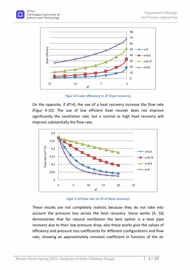
Department of Energy
and Process engineering
Master thesis Spring 2011: Analyzes of Solar Chimney Design 4—59
Figur 4-9 solar efficiency Vs dT (heat recovery)
On the opposite, if dT>0, the use of a heat recovery increase the flow rate
(Figur 4-10). The use of low efficient heat recover does not improve
significantly the ventilation rate, but a normal or high heat recovery will
improve substantially the flow rate.
Figur 4-10 Flow rate Vs dT>0 (heat recovery)
These results are not completely realistic because they do not take into
account the pressure loss across the heat recovery. Some works [4, 16]
demonstrate that for natural ventilation the best option is a heat pipe
recovery due to their low pressure drop; also these works give the values of
efficiency and pressure loss coefficients for different configurations and flow
rate, showing an approximately constant coefficient in function of the air
0
10
20
30
40
50
60
70
80
-17 -12 -7 -2
Sola
r ef
fici
ncy
dT
e=0
e=0,4
e=0,75
e=0,9
0
0,05
0,1
0,15
0,2
0,25
0,3
0 5 10 15 20 25
Flo
w r
ate
(m^^
/s)
dT
e=0,4
e=0,75
e=0,9
e=0

Department of Energy
and Process engineering
Master thesis Spring 2011: Analyzes of Solar Chimney Design 4—60
velocity. The best, the worst and the normal cases was taken to calculate the
flow rate in the building and compare without heat recovery.
Figur 4-11 Flow rate Vs dT (heat pipe recovery)
Figur 4-11 shows that a heat recovery with a low pressure drop decreases
considerably the air exchange and only, in case when dT is enough high, the
heat recovery, make sense to use it. On the other hand, if the building is
design with control valve that allows controlling the pass through the heat
recovery of the air in function of the difference of temperature; the
possibilities of the recuperator increase.
0
0,1
0,2
0,3
0,4
0,5
0,6
0,7
0,8
0,9
-16 -6 4 14
Flo
w r
ate
(m^3
/s)
dT
e=0.3 & k=4
e=0.5 & k=2
e=0.4 & k=3
non recovery

Department of Energy
and Process engineering
Master thesis Spring 2011: Analyzes of Solar Chimney Design 5—61
5 Further work The solar chimney installed in the EPT-lab is a new design and no so much
information can be found. Therefore, it is important to continue the work
carried out in this Thesis to achieve the design and to understand better the
behavior of the solar chimney.
A 3D CFD simulation with external radiation, to know if the
supposition of uniform temperature and velocity can be applied in
all angles of incident of solar radiation.
Verify the equation 3.6 for a range of angles of solar radiation
Study and simulate different designs of chimney outlets to improve
the wind effect in the solar chimney.
A non-steady simulation of the chimney to know the behavior of the
chimney in dynamics conditions, for example the thermal energy
storage of the chimney along the day that allows keeping a flow rate
during part of the night.

Department of Energy
and Process engineering
Master thesis Spring 2011: Analyzes of Solar Chimney Design 6—62
6 Conclusion This report study the basic principles of solar chimney and especially the
chimney installed in EPT-lab, utilizing as tools a commercial CFD software,
Fluent, and basic physical models.
The following conclusion could be drawn.
A simple CFD model, without external radiation is enough to
simulated and study with a good accuracy the solar chimney
installed in the EPT-lab.
The design of the solar chimney in the EPT-lab allows to use simple
physical models, to know its properties (flow rate and temperature)
and also to model the size (height and solar collector area), due to
the uniform velocity and temperature that appears inside the
chimney. Also these characteristics of the flow make it possible use
all the knowledge of the standard chimneys in this solar chimney.
The EPT- solar chimney can be used in both types of climates
(warmer and cold) and for reasonable height it is the type of solar
chimney which gives the highest flow rate. Only in warmer climates
and in high buildings the solar chimney type 3 will give better
results.
The solar efficiency of the chimney depends of the magnitude of
solar radiation, but also of the difference of temperatures between
the building and the surroundings. Therefore, only in the cases
where the difference of temperature is near to zero, the solar
chimney makes sense to use it.
The height of the chimney is usually important to increase the flow
rate, but in the cases when the temperature inside the building is
lower than the external it is more important to increase the area of
the solar collector than the height of the chimney.
A solar chimney with a heat recovery improves the solar efficiency
of a building but hinders the air exchange. For that reason, only
hybrid ventilation systems with the support of a fan and with the
enough flexibility to change the course of the flow rate should be
used with the solar chimney and a heat recovery.

Department of Energy
and Process engineering
Master thesis Spring 2011: Analyzes of Solar Chimney Design 7—63
7 References 1. Clito Oliveira, A.A., Solar chimneys: simulation and experiment.
Energy and Buildings, 2000. 32(1): p. 71-79. 2. Khedari, J., B. Boonsri, and J. Hirunlabh, Ventilation impact of a solar
chimney on indoor temperature fluctuation and air change in a school building. Energy and Buildings, 2000. 32(1): p. 89-93.
3. Szikra, C., Hybrid ventilation systems. 2002, Budapest University of Technology and Economics.
4. Gan, G. and S.B. Riffat, A numerical study of solar chimney for natural ventilation of buildings with heat recovery. Applied Thermal Engineering, 1998. 18(12): p. 1171-1187.
5. I. Chand and P. Bhargava, Studies on design and performance of a non-conventianal system of natural ventilation in buildings. Solar and Wind Technology 1990.
6. Ong, K.S., A mathematical model of a solar chimney. Renewable Energy, 2003. 28(7): p. 1047-1060.
7. Sakonidou, E.P., et al., Modeling of the optimum tilt of a solar chimney for maximum air flow. Solar Energy, 2008. 82(1): p. 80-94.
8. Dai, Y.J., et al., Enhancement of natural ventilation in a solar house with a solar chimney and a solid adsorption cooling cavity. Solar Energy, 2003. 74(1): p. 65-75.
9. Agung Murti Nugroho and M.H.b. Ahmad, POSSIBILITY TO USE SOLAR INDUCED VENTILATION STRATEGIES IN TROPICAL CONDITIONS BY COMPUTATIONAL FLUID DYNAMIC SIMULATION. 2005: p. 8.
10. Åke Blomsterberg, Åsa Wahlström, and M. Sandberg, Refurbishment of the Tånga school. 2002, INTERNATIONAL ENERGY AGENCY, ENERGY CONSERVATION IN BUILDINGS AND COMMUNITY SYSTEMS.
11. Daivid Etheridge and M. Sandberg, Pressure Differences generated by Temperature, in Building Ventilation: Theory and Measurement
1996. p. 28-29. 12. http://www.brynmawr.edu/geology/206/gruenstein2.htm. Solar
Tower Technology. 13. http://en.wikipedia.org/wiki/Cubic_function. Cubic function. 14. Carmen Viñas, et al., Analysis of the Behavior of a Turbulent Jet
Indoor. Informacio Tecnológica, 2008. 19 Nº5: p. 9. 15. ANSYS, I., ANSYS FLUENT 12.0 Theory Guide. 2009. 816. 16. Shao, L., S.B. Riffat, and G. Gan, Heat recovery with low pressure loss
for natural veltilation. Energy and Buildings, 1998. 28(2): p. 179-184.

Department of Energy
and Process engineering
Master thesis Spring 2011: Analyzes of Solar Chimney Design 7—64
17. Störm, H.C., CFD investigation of flow in and around a natural draft cooling tower, in Mechanical and Mechatronic Engineering 2010.
[1, 3, 8, 9, 11, 14, 15, 17]

- 1 -
Appendix 1
Pressure Loss Coefficients and Moody Diagram
Inlets
Outlets
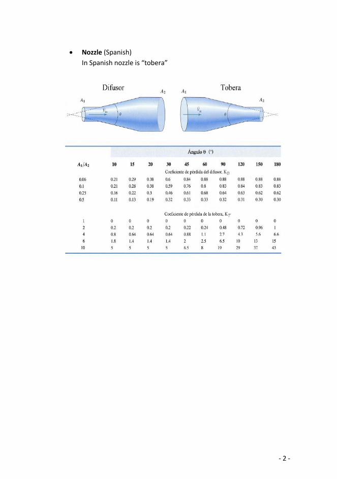
- 2 -
Nozzle (Spanish)
In Spanish nozzle is “tobera”
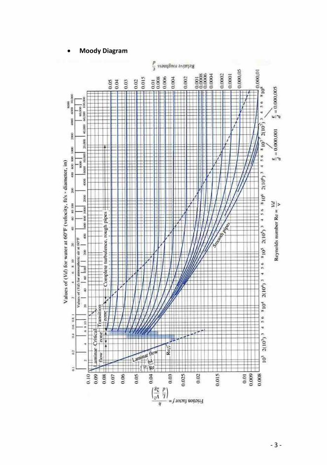
- 3 -
Moody Diagram

- 4 -
Appendix 2
Window data
Position outside
Glass type Thickness mm Weight kg/m2
Glass 1 OptifloatTM Clear 4 10 Space 90% Argon Glass2 OptithermTM SN 15 10
Product code Type Thickness mm Weight kg/m2
4-15Ar-SN4 2 23 20

- 5 -
Appendix 3
Solar Chimney EPT-lab
Chimney side
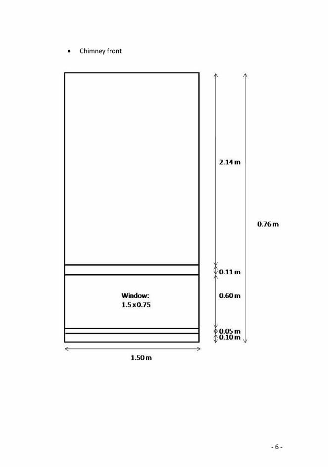
- 6 -
Chimney front

- 7 -
Sola collector and fins
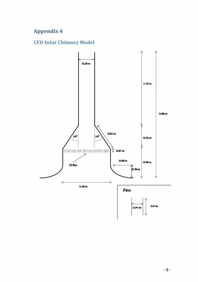
- 8 -
Appendix 4
CFD Solar Chimney Model

- 9 -