analyzing earthquake casualty risk at … · 2014-07-18 · analyzing earthquake casualty risk at...

ANALYZING EARTHQUAKE CASUALTY RISK AT CENSUS BLOCK LEVEL:

A CASE STUDY IN THE LEXINGTON CENTRAL BUSINESS DISTRICT,

KENTUCKY

by

Jarod Thomas Hustler

A Thesis Presented to the

FACULTY OF THE USC GRADUATE SCHOOL

UNIVERSITY OF SOUTHERN CALIFORNIA

In Partial Fulfillment of the

Requirements for the Degree

MASTER OF SCIENCE

(GEOGRAPHIC INFORMATION SCIENCE AND TECHNOLOGY)

August 2014

Copyright 2014 Jarod Thomas Hustler

ii

DEDICATION

This work is dedicated to all of the hard working individuals who put themselves in

harm’s way to help others in distress. This includes, but is not limited to, the first

responders, disaster relief volunteers and all of those who help support them in difficult

times. God Bless you and it is my hope that this study can improve upon your future

heroic efforts.

iii

ACKNOWLEDGMENTS

I would like to thank my thesis chair, Dr. Flora Paganelli, for her assistance in this long

process. I really appreciate all of the support and guidance she has provided to complete

this project. I would also like to thank my thesis committee members, Dr. Su Jin and Dr.

Yao-Yi Chiang, and everyone within the SSI department at USC that has helped me

throughout the entire Master’s program. Thank you to Dr. Junfeng Zhu of the Kentucky

Geological Survey for providing the LiDAR data created by Photo Science, Inc.

iv

Table of Contents

DEDICATION................................................................................................................... ii

ACKNOWLEDGMENTS ............................................................................................... iii

LIST OF TABLES ........................................................................................................... vi

LIST OF FIGURES ........................................................................................................ vii

LIST OF ABBREVIATIONS ....................................................................................... viii

ABSTRACT ...................................................................................................................... ix

CHAPTER 1: INTRODUCTION AND LITERATURE REVIEW ............................. 1

1.1Introduction .......................................................................................................................... 1 1.2.1 Earthquake Studies Using Remote Sensing – Light Detection and Ranging (LiDAR) .. 5

1.2.2 Earthquake Studies Using GIS: HAZUS Application .................................................... 7

1.2.3 Population Estimation Studies ....................................................................................... 9

CHAPTER 2: STUDY AREA AND SEISMIC HISTORY OF AREA ...................... 12

2.1 Study Area .......................................................................................................................... 12

2.2 Seismic History of the Study Area ................................................................................... 13 2.2.1 New Madrid Seismic Zone (NMSZ) .............................................................................. 13

2.2.2 Wabash Valley Seismic Zone ........................................................................................ 14

2.2.3 Earthquakes and Faults Near the Study Area .............................................................. 15

CHAPTER 3: DATA SOURCES AND METHODOLOGY ....................................... 17

3.1 Data Sources ....................................................................................................................... 18 3.1.1 Census Data ................................................................................................................. 18

3.1.2 LiDAR Data .................................................................................................................. 19

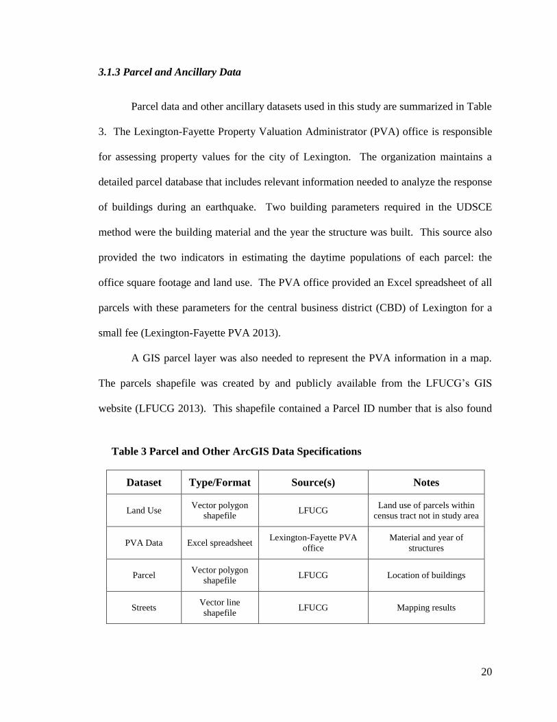
3.1.3 Parcel and Ancillary Data ........................................................................................... 20

3.2 Pre-processing Data ........................................................................................................... 21 3.2.1 Census Pre-processing: Estimating Daytime Populations By Parcel .......................... 21

3.2.2 Pre-processing LiDAR Data ........................................................................................ 23

3.2.3 Pre-processing Parcel Data ......................................................................................... 24

3.2.4 Changes to Pre-processing Based on Study Area Data Acquisition ............................ 25

3.3 Methodology ....................................................................................................................... 27 3.3.1 HAZUS-MH Methodology ............................................................................................ 28

3.3.2 UDSCE Method at Census Tract Level ........................................................................ 30

3.3.3 UDSCE Method at Census Block Level ....................................................................... 36

CHAPTER 4: RESULTS ............................................................................................... 38

4.1 HAZUS-MH Results .......................................................................................................... 39

4.2 UDSCE Method at Census Tract Level Results .............................................................. 42 4.2.1 Validation of UDSCE Method ...................................................................................... 43

4.3 UDSCE Method at Census Block Level Results ............................................................. 45

4.4 UDSCE Method at Parcel Level Results ......................................................................... 47

CHAPTER 5: CONCLUSIONS AND FUTURE WORK ........................................... 49

5.1 Conclusions ........................................................................................................................ 49

5.2 Future Work ...................................................................................................................... 50 5.2.1 Data Availability .......................................................................................................... 51

5.2.2 Flexibility of UDSCE Method ...................................................................................... 51

v

5.2.3 Study Area Constraints................................................................................................. 52

5.2.4 Population Estimations ................................................................................................ 52

5.2.5 Time Factors Affecting Estimates ................................................................................ 53

REFERENCES ................................................................................................................ 54

APPENDIX A: Indoor Casualty Rates by Model Building Type for Slight Structural

Damage............................................................................................................................. 58

APPENDIX B: Indoor Casualty Rates by Model Building Type for Moderate

Structural Damage .......................................................................................................... 59

APPENDIX C: Indoor Casualty Rates by Model Building Type for Extensive

Structural Damage .......................................................................................................... 60

APPENDIX D: Indoor Casualty Rates by Model Building Type for Complete

Structural Damage (No Collapse).................................................................................. 61

APPENDIX E: Indoor Casualty Rates by Model Building Type for Complete

Structural Damage (With Collapse) .............................................................................. 62

APPENDIX F: Explanation of Building Types ............................................................ 63

vi

LIST OF TABLES

Table 1: Census Data Specifications 19

Table 2: LiDAR Data Characteristics 19

Table 3: Parcel and Other ArcGIS Data Specifications 20

Table 4: Breakdown of Office Worker Population by Census Tract 23

Table 5: Alternate Formats of Datasets Used For UDSCE Method 26

Table 6: Description of Injury Severity Levels for HAZUS-MH 28

Table 7: HAZUS-MH Default Setting For Population Distribution 29

Table 8: Building Material Scores 32

Table 9: Building Height Scores 33

Table 10: Building Age Scores 34

Table 11: Total Score Ratings 34

Table 12: UDSCE Casualty Rates by Damage State 35

Table 13: Examples of Vulnerability Calculation by Parcel 36

Table 14: Examples of Casualty Calculation by Parcel 36

Table 15: HAZUS-MH Casualty Estimates for 5.5 Magnitude

Earthquake 40


Earthquake 41


Earthquake 41

Table 18: UDSCE Method For Study Area Results 43

Table 19: Comparison of HAZUS-MH and UDSCE Results 44

Table 20: Percent Difference Error Analysis of Results 45

vii

LIST OF FIGURES

Figure 1: LiDAR Image of Urban Area 6

Figure 2: Study Area Map 12

Figure 3: Map of Fault Lines in Central Kentucky 16

Figure 4: Workflow of Earthquake Casualty Estimation 17

Figure 5: Map of Office Square Footage for Census Tract 22

Figure 6: Raw LiDAR Points of Study Area 24

Figure 7: LiDAR Preprocessing Flowchart 25

Figure 8: Parcel Preprocessing Flowchart 26

Figure 9: Map of Study Area Parcels 27

Figure 10: HAZUS-MH Earthquake Methodology Flowchart 29

Figure 11: UDSCE Method Flowchart 31

Figure 12: Modelbuilder Design of UDSCE Method by Census Tract 37

Figure 13: Modelbuilder Design of UDSCE Method by Census Block 37

Figure 14: Map of Earthquake Epicenter 38

Figure 15: HAZUS-MH Total Casualty Maps by Magnitude 40

Figure 16: UDSCE Method Total Casualties in Study Area Map 42

Figure 17: Estimation of Casualties by Census Block 46

Figure 18: Census Block Casualties by Land Use 46

Figure 19: Estimation of Casualties by Parcel 48

viii

LIST OF ABBREVIATIONS

CBD Central Business District

CUSEC Central United States Earthquake Consortium

FEMA Federal Emergency Management Agency

GIS Geographic Information Systems

HAZUS-MH Hazards United States Multi-Hazard

KGS Kentucky Geological Survey

KRFS Kentucky River Fault System

LFUCG Lexington-Fayette Urban County Government

LiDAR Light Detection and Ranging

NEHRP National Earthquake Hazards Reduction Program

NMSZ New Madrid Seismic Zone

PDE Percentage Difference Error

PVA Property Valuation Administrator

UDSCE Urban Daytime Seismic Casualty Estimation

USGS United States Geological Survey

WVSZ Wabash Valley Seismic Zone

ix

ABSTRACT

Earthquakes strike without warning and leave a trail of devastation. To better

prepare for these disastrous events, government agencies must have a comprehensive

emergency management plan based on current spatial and non-spatial data. Applications

such as HAZUS-MH, developed by the Federal Emergency Management Agency

(FEMA), can be used with ArcGIS software to model loss estimations for many natural

disaster scenarios. However, HAZUS-MH does not supply the necessary data to analyze

losses at geographic units smaller than the census tract level, limiting its effectiveness for

an urban area earthquake casualty study.

Focusing on the Central Business District (CBD) of Lexington (Kentucky), this

study developed a new methodology to test alternate input such as locally sourced

LiDAR remote sensing data and Geographic Information System (GIS) -based parcels

data to predict earthquake casualties within an urban area. The Urban Daytime Seismic

Casualty Estimation (UDSCE) method was applied at a census tract level and casualty

estimations validated using the HAZUS-MH model results from three simulated

earthquake scenarios. The UDSCE methodology was then applied at the census block and

parcel level to refine estimates counts at higher resolution.

The results show compelling evidence that working at the census block and parcel

level can provide focalized casualty counts within the urban context, thus providing

emergency planners crucial information to better prepare for earthquake events in

commercial/urban densely populated areas.

CHAPTER 1: INTRODUCTION AND LITERATURE REVIEW

Chapter 1 provides an introduction on my personal interest in earthquake hazard events

and the importance of earthquake hazard modeling and damage estimates made possible

with advanced technologies such as GIS. This is followed by a literature review in

relation to earthquake hazard events and damage estimates using Remote Sensing and

GIS is provided. The chapter ends with summary of the key the research questions and

objectives of this thesis.

1.1 Introduction

I will never forget the first time I felt an earthquake. I was a fifth grader living in

Southern California when a strong tremor hit the city of Whittier on the morning of 1

October, 1987. As I was getting dressed for school in my bedroom, everything around

me started shaking. Initially I was frozen in place; after a few seconds my instincts

kicked in and I climbed under my desk for safety. The many practice drills that my

school conducted in preparation for an earthquake were finally put to the test.

Fortunately, I lived far enough away from the epicenter to not experience any damage to

my house and I was able to go to school. There were lots of interesting conversations

that day with my classmates about what they experienced during the event. Some even

wrote out their last wills!

A couple years after that experience I moved across the country, where

earthquakes are virtually non-existent. I felt I would never have to worry again about

being ready for an earthquake. I was wrong. A scientist predicted that a large earthquake

would strike along the New Madrid Seismic Zone (NMSZ) in Missouri, potentially

2

affecting the community that I now called home (Show Me Net 2014). Many area school

districts shut down that day, and even though my school was open, a large percentage of

children stayed home. The predicted earthquake never happened and life went on as

normal after that day.

These two events in my life, though completely opposite in nature, were stark

reminders of the importance of being ready for disaster to happen at any time. In the first

case, I had no warning of the impending seismic event. The benefit was that careful pre-

planning allowed me to make an informed decision to protect myself the best I possibly

could at that very moment. The second event (or lack thereof) frightened many people

who were not sure what to do if the earthquake took place. Many questions were raised

in my mind regarding the second event that I still think about to this day. What would

have happened if there was an earthquake that day? Would the kids that stayed home that

day have had a better chance of surviving than the ones that went to school? Did state

and local emergency managers have the resources necessary at that time to deal with this

kind of disaster to limit casualties? If so, were they flexible enough to make any changes

to their execution of the plan if the disaster took place at a different time of day? These

questions are difficult at best to answer unless the event actually took place, putting the

emergency workers to the test.

As time has passed, technological advances have given researchers better

perspective to answer these questions. Geographic information systems (GIS) software

became a leader in combining data and methodologies to assess disaster risk such as

casualties stemming from an earthquake (Esri 2008). The majority of injuries and deaths

attributed to earthquakes are due to the damage of buildings and structures where people

3

are located at the time of the event (USGS 2014). In that regard, having accurate

information of building structures and headcounts within those structures to add into a

GIS database can lead to better prediction of casualties and their spatial distribution

within the area of study.

Despite the rapid advancement of the capabilities to look at risk from seismic

activity, there are several issues within the scientific community that impede the progress

of the effectiveness of incorporating GIS in earthquake studies. For one, GIS and remote

sensing technology show little, if any, improvement in predicting when and where an

earthquake will take place (Gillespie et al. 2007). This limitation still leaves the study of

estimating damages as purely hypothetical and many earthquake scenarios would have to

be viewed for a particular study area, adding cost and time to such projects. Models

could be validated with historical earthquake events, but finding damage assessment data

for an area that suffered an earthquake with enough similarities to any study location

would be difficult. More significantly, Geiβ and Taubenböck (2013) confess that there is

an absence of consistent definitions of key terms such as “risk” and “vulnerability”

among researchers in the field. As a result, separate studies of similar scope and scale

can have drastically different results, making it hard to decide which model would be the

best one on which to base a disaster response.

One way to sidestep these concerns is to use a comprehensive modeling system

with a standardized methodology that houses its own data. The Federal Emergency

Management Agency (FEMA) has implemented such a system that is capable of running

efficient models of major disasters throughout the United States. Called HAZUS-Multi

Hazard (MH), the application works in conjunction with ArcGIS software and can be

4

used by any GIS professional or government organization that is interested in

understanding how disasters such as earthquakes, floods, and hurricanes could impact

their communities (FEMA 2014). FEMA works in partnership with the National

Earthquake Hazards Reduction Program (NEHRP), creating and sharpening strategies to

better prepare the United States for earthquakes (NEHRP 2014). This collaboration relies

heavily on HAZUS-MH to achieve their stated goal of reducing loss of life and property

damage due to earthquakes.

The database that is included with HAZUS-MH contains the best available

engineering information for buildings (HAZUS-MH 2013). Also included is

demographic data to analyze physical, social and economic losses from earthquakes

(FEMA 2014). Thousands of historical earthquakes for the United States are included in

the data so researchers could try to see what damage a subsequent earthquake would

cause. HAZUS-MH can also accept outside data input so more experienced GIS users

can analyze losses with more trusted and detailed information that they may possess.

HAZUS-MH outputs include maps, charts, and reports that can convince any state,

county or municipality to support and implement important safeguards in case a disaster

strikes.

HAZUS-MH is a fascinating tool for disaster modeling and it can fill many needs

when crafting the right emergency plan for any place, but it can be improved upon.

HAZUS-MH is only equipped to model losses at a census tract level or larger. This

poses a problem for modeling an earthquake scenario of casualties for many densely

populated urban areas, where more detailed losses at a census block group level, census

block level or even a parcel level would be desirable. These higher resolution levels help

5

find the way the casualties are distributed by units contained in the census tract. Though

GIS professionals can generally overcome this limitation in the standard HAZUS-MH

application by introducing additional data input such as more detailed building

characteristics and demographic distribution, novice users would struggle with obtaining

better data or know how to leverage the data in HAZUS-MH if they did have it available.

Hopefully there would be an opportunity for less experienced users to apply this useful

methodology to demographic data not already tied into the application.

1.2 Literature Review

This section contains a full literature review of related studies of estimating

earthquake damages. Many studies of earthquake vulnerability utilized GIS software for

analysis (Sahar, Muthukumar and French 2010, Hashemi and Alisheikh 2011, Aydöner

and Maktav 2009); several of which cited HAZUS-MH as a part of their process (Remo

and Pinter 2012, Ploeger, Atkinson and Samson 2010, Neighbors et al. 2013). As this

thesis explores estimating casualty counts, a review of population estimation studies have

also been included here.

1.2.1 Earthquake Studies Using Remote Sensing – Light Detection and Ranging

(LiDAR)

The use of Light Detection and Ranging (LiDAR) remote sensing technology has

become increasingly popular in mapping the earth’s surface. The process involves using

a laser scanner attached to an aircraft that is aimed at the ground. The scanner shoots

millions of laser pulses to determine an accurate depiction of the topography of the land

below (and typically include tree canopies, buildings and other large objects). Figure 1

shows what a LiDAR scan of an urban area would look like. The calculation of the time

6

it takes for each pulse to travel to the surface of the earth and back to the source is then

converted to elevation figures for the surface (Campbell and Wynne 2011, 245).

LiDAR data holds several uses for studying urban environments. Sampath and

Shan (2007) used a modified convex hull approach to trace building footprints from

LiDAR data in multiple urban settings. They documented how point spacing (resolution)

of the LiDAR datasets and other factors such as building angles affected the

regularization process that led to errors in the final output. Barazzetti, Brovelli and

Valentini (2010) introduced a method that uses LiDAR data to correct errors inherent to

aerial photos, including vertical displacement. Their results showed promise, especially

for working with orthophotos of urban areas where tall buildings often distort the image.

Other types of remote sensing have been proven to demonstrate effective analysis

of earthquake damage and vulnerability. Two examples are comparing pre- (5 meter

Figure 1 LiDAR Image of Urban Area

Source: http://oginfo.com/images/lidar_2_610.png

Accessed 15 April 2014

7

resolution) and post-earthquake (2.5 meter resolution) SPOT-5 panchromatic satellite

images to recognize damaged structures (Dell’Acqua and Gamba 2012) and the use of

radar-based tools to analyze changes in digital elevation models (DEM) of landscapes

affected by an earthquake (Geiβ and Taubenböck 2013, Liu et al. 2012). Despite its

growing popularity, LiDAR has not had much utilization in earthquake damage and

vulnerability studies. One possible reason for this is the ability to easily transform

general building stock data as a substitute input. Hashemi and Alisheikh (2011)

demonstrated this by using building stock data of a district in Tehran, Iran and making

3D images of each structure based on the number of stories for earthquake analysis.

Fragility curves were created from the building materials data of the structures within the

study area and a model was implemented to try to predict building damage, casualty

counts and street blockages in the event of an earthquake occurring on the Mosha Fault

nearby. The model was verified by analyzing actual damage and casualty data from the

massive earthquake that damaged much of the city of Bam, Iran in 2003. Since there was

not a good database available for Bam as there was for the district of Tehran, the results

of the comparison were questionable. The upside was that the model does still identify

likely points of destruction and street blockage, which can still contribute to working

toward mitigating losses in case of an actual earthquake.

1.2.2 Earthquake Studies Using GIS: HAZUS Application

One feature of HAZUS-MH is the ability to supply supplemental data for

earthquake loss analysis, giving users opportunities to compare results between their own

data and what is already included when scenarios are played out. Remo and Pinter

(2012) tried multiple soil maps to help predict losses for a potential large earthquake in

8

southeast Illinois. Their studies consistently showed that HAZUS-MH data

overestimated damages and casualties compared to user-supplied data. Ploeger, Atkinson

and Samson (2010) ran a HAZUS-MH model on potential damages that would occur if a

strong earthquake were to strike near Ottawa, Canada. Despite extra steps required to

overcome using an application designed for the U.S. in an international setting, the study

helped identify areas of the city center that could receive the most damage from an

earthquake. Moffatt and Cova (2010) used parcel data for all of Salt Lake County, Utah

to try to predict economic loss estimates for each residential unit under a potential

earthquake threat. They found that this was a massive undertaking given the amount of

data involved. HAZUS-MH alone was not sufficient to run the analysis, so they used an

alternate software package using the same methodology. The large scope of the project

(almost 250,000 parcels analyzed) required additional computer hardware and scripting

tools so the modeling could be completed in a reasonable amount of time.

Historical earthquakes can also be modeled in current times with HAZUS-MH.

Neighbors et al. (2013) took this approach and analyzed both HAZUS-MH and user

supplied data for a handful of earthquakes that occurred around King County,

Washington in the past several decades. Again, HAZUS-MH supplied data

overestimated losses compared to datasets brought in from outside sources. Kirscher,

Whitman and Holmes (2006) used actual reported losses from the 1994 Northridge,

California earthquake to see how close HAZUS-MH could estimate those losses. Though

deaths were overestimated and serious injuries were underestimated, many of the

estimated economic losses lined up closely to reported residential insurance claims that

were paid.

9

1.2.3 Population Estimation Studies

Much like building vulnerability prediction, remote sensing is useful for

population estimation studies. Dong, Ramesh and Nepali (2010) used ordinary least

squares (OLS) regression methodologies to predict populations in Denton, Texas. Light

Detection and Ranging (LiDAR) remote sensing data provided footprints and building

heights and parcel data was used to filter out non-commercial and non-residential areas.

Landsat TM was also included and helped establish land use for this study. Many of their

estimations turned out to be lower than actual numbers as issues like spatial resolution

discrepancies between LiDAR and Landsat and difficulty distinguishing between trees

and structures in the LiDAR that was used caused some error. Qiu, Sridharan and Chen

(2010) also looked at OLS for their population estimation study in Round Rock, Texas.

Due to spatial autocorrelation leading to a higher incidence of Type I error, they opted to

compare those results to spatial autoregressive models and witnessed a big improvement

in their estimations. Silván-Cárdenas et al. (2010) tested four different algorithms on

their remote sensing data to detect buildings and several methods of land use

classification for areas of Austin, Texas. Their resulting population estimations

suggested that overall accuracy assessments using the methods tested would improve if

bias from estimated building attribute information were reduced.

Some of the same strategies used on these studies can also be applied to

estimating the number of workers in an office building. Knowing these counts would be

particularly useful for studying earthquake casualty counts in urban areas given the event

takes place in the daytime. One such study conducted by Miller (2012) looked at trends

of the amount of office space that is needed for each worker and breaks down some

10

estimations of office space per worker for many U.S. cities in addition to breakdown by

various industries. This study did not utilize GIS; however, it gives important insight into

developing a formula to calculate office worker numbers for buildings contained within a

study area.

1.3 Research Question and Objectives

How effective would be the estimate of earthquake casualty counts obtained at a

census block level for a downtown business district if the event took place during the

daytime, when the study area contains the highest population count? HAZUS-MH

methodology was used as a comparative tool for the Urban Daytime Seismic Casualty

Estimation (UDSCE) customized application process using locally-sourced spatial data

such as Light Detection and Ranging (LiDAR) data, parcels and property valuation

assessor (PVA) data to generate all of the individual building parameters necessary to

assess the overall vulnerability of each building. The UDSCE method is a newly built

model designed to predict the distribution of estimated casualties in an urban

environment. In a controlled scenario, the comparative analysis between HAZUS-MH

and the UDSCE method was used to achieve the following measureable objectives:

validation of the UDSCE method at the census tract level through

comparison with the HAZUS-MH model results;

higher resolution analysis using the UDSCE approach at a census block level;

comparison of the UDSCE results at census tract, census block and parcel

level.

The remainder of this thesis is divided into four chapters. Chapter 2 describes the

study area in great detail and the importance of selecting this particular area for the stated

objectives. Chapter 3 details the HAZUS-MH methodology and data that is included,

11

then introduces the UDSCE method and the data input used for the comparative analysis.

Chapter 4 reports the findings of the spatial distribution of casualties by census block

using the UDSCE method and identifies how it differs from the results of the census tract

test are reported. Chapter 5 points out which areas of the study went well and which did

not work, and it debates whether the UDSCE approach can be considered as an

improvement over the current HAZUS-MH model.

12

CHAPTER 2: STUDY AREA AND SEISMIC HISTORY OF AREA

Chapter 2 introduces the study area and provides a brief discussion of past seismic events

that occurred near the study area as a context for this study.

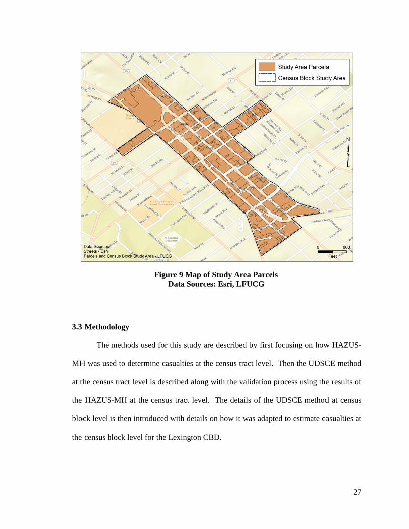
2.1 Study Area

The Central Business District (CBD) of Lexington, Kentucky has been selected as

the study area for this experiment. The area is defined by 52 census blocks containing a

total of 345 parcels that were analyzed for earthquake casualties under the UDSCE

Figure 2 Study Area Map

Data Sources: Esri and LFUCG

13

method. Figure 2 illustrates the census block study area plus the boundary of census tract

#21067000100, with a commercial working (daytime) population of 10,713, according to

the 2000 census survey (U.S. Census 2013). This is the most current estimation of office

workers available for this area and is already included with the data available to users of

HAZUS-MH.

2.2 Seismic History of the Study Area

Lexington is not known for seismic activity, but its residents could be in more

danger than most people realize. This section summarizes the history of notable

earthquakes that have affected the state of Kentucky, including zones in neighboring

states where future activity can still cause major damage for hundreds of miles around.

2.2.1 New Madrid Seismic Zone (NMSZ)

The NMSZ in southeast Missouri is the location of one of the largest earthquakes

in U.S. history. A series of earthquakes occurred over the winter months of 1811-1812

along the NMSZ that devastated the sparsely populated region and disrupted the flow of

the Mississippi River for several days. Each quake was believed to be in the magnitude

range of 7.5 – 8.0, and one tremor caused church bells to ring 1,000 miles away in Boston

(CUSEC 2013). Damage was reported in other faraway places, including Washington,

D.C. and Charleston, South Carolina.

Scientists state that the probability of a magnitude 6.0 or higher earthquake

occurring here in the next 50 years is between 25-40 percent (CUSEC 2013). An event

of that magnitude happening again along the NMSZ would affect a much larger

14

population base that is not accustomed to dealing with seismic activity. The metropolises

of Memphis, Tennessee and St. Louis, Missouri would be particularly vulnerable to large

numbers of casualties as a result of future events in this zone. Lexington is located 400

miles to the northeast of the NMSZ, but the city is not far enough away to escape danger

if future activity here is as strong as or stronger than the events of 1811-1812.

2.2.2 Wabash Valley Seismic Zone

The Wabash Valley Seismic Zone (WVSZ) is found along the Illinois-Indiana

border where the Wabash River serves as the dividing line between the two states. Some

recent moderate earthquakes centered within the zone have resulted in damage to

structures in the state of Kentucky. A 5.2 magnitude earthquake centered near Mt.

Carmel, Illinois on 18 April, 2008 was reviewed by Remo and Pinter (2012) in their

HAZUS-MH study. This tremor caused a brick façade to collapse in Louisville,

Kentucky, 150 miles to the east, but no injuries were reported in the state (The Business

Journals 2008). A 5.4 magnitude earthquake that took place on 9 November, 1968 in the

area did significant damage to the masonry of the City Building in Henderson, Kentucky,

50 miles away (USGS 2014).

The WVSZ is much closer to Lexington than the NMSZ at a distance of 250

miles. Recent history shows that it has been much more active as well. Though recent

earthquakes in the WVSZ have not been as strong as what its counterpart has been known

to produce, the possibility remains that this area is capable of stronger earthquakes in the

future. Geologist Steven Obermeier found evidence of liquefaction (the process of

seismic shaking turning soil into a substance similar to quicksand) within the zone in the

15

mid-1980’s and believes that it was caused by an earthquake about 6,100 years ago at the

estimated magnitude of 7.1 (CUSEC 2013).

2.2.3 Earthquakes and Faults Near the Study Area

Earthquakes that originated in the state of Kentucky were rarely moderate or

strong in magnitude. Many of these tremors happened in the western half of the state,

which were closer in proximity to the NMSZ and the WVSZ and were most likely not felt

in Lexington. However, sporadic seismic activity has been observed in the northeastern

part of the state for the last 150 years (Mauk, Christensen and Henry 1982). It was in this

region where the state’s strongest earthquake occurred. The event took place near

Sharpsburg on 27 July, 1980, a mere 40 miles to the northeast of Lexington. This tremor

measured 5.2 on the Richter scale and caused $3 million worth of damage ($8.4 million

today) to hundreds of homes and businesses in and around the city of Maysville, 60 miles

from Lexington (Street 1982).

Earthquake faults do exist in the immediate area around Lexington. The best

visual evidence of fault lines are found along the Kentucky River fault system (KRFS).

This system of fault lines run primarily east-west across the state of Kentucky, and gets

as close as 15 miles to the CBD of Lexington (Vanarsdale 1986). Figure 3 shows the

location of the KRFS and other fault lines in relation to the city of Lexington (LFUCG

2013).

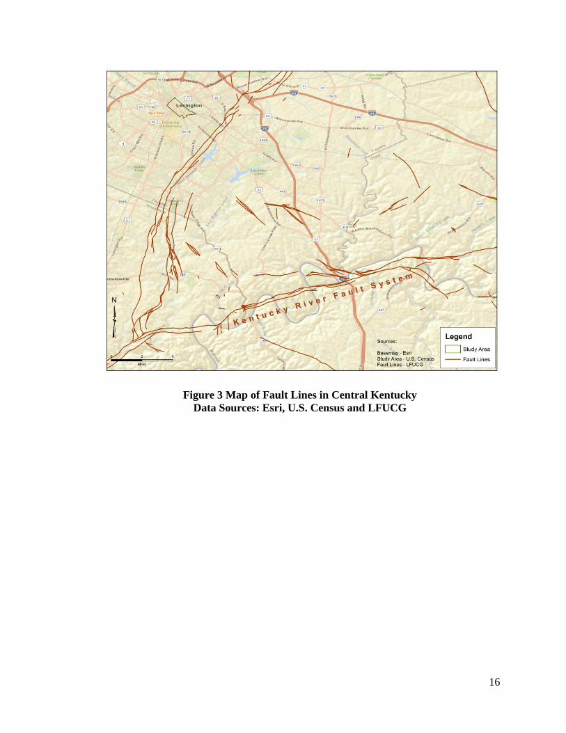
16

Figure 3 Map of Fault Lines in Central Kentucky

Data Sources: Esri, U.S. Census and LFUCG

17

CHAPTER 3: DATA SOURCES AND METHODOLOGY

Chapter 3 introduces the data types, sources, and pre-processing required for them to be

used in this study. This is followed by the methodology subsection, which outline in

detail the HAZUS-MH and UDSCE methods for earthquake casualty estimations used for

this study.

The workflow followed in this study is summarized in Figure 4. This workflow

outline the HAZUS-MH and UDSCE earthquake casualty models, the validation process

of the results of the UDSCE versus HAZUS-MH models and relative percentage

difference error estimation, the final steps in the UDSCE’s higher level casualties

Figure 4 Workflow of Earthquake Casualty Estimation

18

computation at block and parcel level.

The HAZUS-MH component used (model defaults) building and population input

and three earthquake magnitude scenarios to produce output used for the validation

process. For the UDSCE component the input data were acquired specifically for this

study and pre-processed, then a scoring method using three parameters of the structure

(building height, age and material) was used to determine the building’s vulnerability

similarly to HAZUS-MH used standards. The UDSCE’s results were validated by

comparison with HAZUS-MH’s output from three earthquake magnitude scenarios,

finally the percentage difference error of the results was computed. Further analysis was

then conducted with the UDSCE method to estimate casualties at higher resolution,

specifically for block and parcel level.

3.1 Data Sources

The data used in this study are divided in three main categories encompassing

census, LiDAR and parcel data. The sources, characterization, and importance of each

data category in relation to this study will follow in this section.

3.1.1 Census Data

Census data were used to derive, with good accuracy, the number of people that

reside in a multitude of geographic units such as states, counties and zip codes. Finer

levels of resolution of census data such as census tracts and census blocks contain precise

population and demographic data for studies of urbanized areas. The census block

shapefile was publicly available through the U.S. Census website (U.S. Census 2013).

19

The census tract used for the study was also created by the U.S. Census and was accessed

through the HAZUS-MH application (HAZUS 2013). The census tract containing the

study area estimates the daytime population for the area, which was critical to help

calculate casualty counts for the study. Table 1 summarizes the census data used.

3.1.2 LiDAR Data

For this study, it was necessary to find the building heights associated with each

parcel as this parameter is a component in determining earthquake vulnerability in

buildings under the UDSCE method. The LiDAR files that were used for this study was

created by Photo Science, Inc. in 2012 and was obtained for free through the Kentucky

Geological Survey (KGS 2013). The data has a resolution of one meter, representing the

spacing of the points during data collection (Table 2).

Table 2 LiDAR Data Characteristics

Dataset Type/

Format Source(s) Resolution

Year

Created Notes

LiDAR Raster

file (.lsa)

Kentucky Geological Survey

(created by Photo Science, Inc.) 1 meter 2012

Building

heights

Table 1 Census Data Specifications

Dataset Type/Format Source(s) Notes

Census Blocks Vector polygon

shapefile U.S. Census

Resolution level for

casualty estimation

Census Tract Vector polygon

shapefile

HAZUS-MH (created by

U.S. Census)

Daytime population

count for study area

20

3.1.3 Parcel and Ancillary Data

Parcel data and other ancillary datasets used in this study are summarized in Table

3. The Lexington-Fayette Property Valuation Administrator (PVA) office is responsible

for assessing property values for the city of Lexington. The organization maintains a

detailed parcel database that includes relevant information needed to analyze the response

of buildings during an earthquake. Two building parameters required in the UDSCE

method were the building material and the year the structure was built. This source also

provided the two indicators in estimating the daytime populations of each parcel: the

office square footage and land use. The PVA office provided an Excel spreadsheet of all

parcels with these parameters for the central business district (CBD) of Lexington for a

small fee (Lexington-Fayette PVA 2013).

A GIS parcel layer was also needed to represent the PVA information in a map.

The parcels shapefile was created by and publicly available from the LFUCG’s GIS

website (LFUCG 2013). This shapefile contained a Parcel ID number that is also found

Table 3 Parcel and Other ArcGIS Data Specifications

Dataset Type/Format Source(s) Notes

Land Use Vector polygon

shapefile LFUCG

Land use of parcels within

census tract not in study area

PVA Data Excel spreadsheet Lexington-Fayette PVA

office

Material and year of

structures

Parcel Vector polygon

shapefile LFUCG Location of buildings

Streets Vector line

shapefile LFUCG Mapping results

21

on the PVA spreadsheet. The merger of the parcel shapefile and the PVA spreadsheet

shaped the final study area of block groups within the census tract that would be analyzed

for casualty estimations.

Two ancillary datasets, a street shapefile and a land use shapefile were also

obtained from the LFUCG GIS website (LFUCG 2013). The land use shapefile was used

to identify land use for areas within the study census tract that was outside of the final

study block area, thus to help refine the daytime population estimations. The street

shapefile has been used as a context to enhance the mapping results.

3.2 Pre-processing Data

Each of the acquired datasets for this study required preprocessing steps before

the data could be used. This section describes in detail the preprocessing for each

dataset.

3.2.1 Census Pre-processing: Estimating Daytime Populations By Parcel

An important element required for the UDSCE analysis was to calculate daytime

populations by parcel, for each office building within the study area, from the census

data. For this purpose, an average number of square feet of office space per worker was

considered and used in the UDSCE method. Figure 5 displays the office square footage

for both the study area and the territory outside of the study area within the census tract

(Lexington-Fayette PVA 2013). The average office space utilized per worker in this

scenario was 351.16 sq. ft., where 92.5 percent of the office space within the census tract

lies in the study area, as shown in Table 4. Using the 2000 U.S. Census figure of daytime

22

commercial population of 10,716 for the entire census tract, the total office workers

within the study area was calculated at 9,912.

As no reliable retail or visitor daytime populations were available for the study,

the 351.16 sq. ft. per person average was also applied to the retail and

hospitality/recreation designated parcels. This process added 5,452 people to the total

daytime population for the study area. Most residential parcels within the study area

were ruled out, based on the assumption that people would not likely be at their residence

in the middle of the day. The two exceptions made were for parcels containing a large

apartment complex. Based on their size, they were given default daytime population

Figure 5 Map of Office Square Footage For Census Tract

Data Sources: Esri, LFUCG (2013) and Lexington-Fayette PVA (2013)

23

values of 100 and 50. Other land use categories that were ruled out due to the assumption

of the daytime scenario were vacant lots, parking structures and church parcels.

3.2.2 Pre-processing LiDAR Data

The LiDAR data were used to derive the building height within each parcel of the

study area. Since the input LiDAR file (.lsa format) is not compatible with ArcGIS, the

conversion tool .lsa file to multipoint data file, available in ArcGIS 10.2, was employed

to convert the data. This conversion resulted in a large multipoint data file covering the

entire area. Then, only the points within the final study area (represented by the area in

dark gray in Figure 5) were extracted using the clip tool. The raw LiDAR data for the

study area are shown in Figure 6.

The z-values (representing elevation) were then extracted from the clipped

multipoint file and spatially joined to the parcel data. The point within each parcel with

the highest z-value was used to establish the elevation for each parcel’s building top.

This practice was used assuming that only one building occupies each parcel within the

study area. A new field was created for the parcel shapefile and populated by subtracting

Table 4 Breakdown of Office Worker Population for Census Tract

Census Blocks Office Worker

Population

Office Sq.

Ft.

Percent

Total

Avg. Office

Space/Worker

Within Study Area 9,912 3,480,428 92.5 351.16

Outside of Study Area 804 282,587 7.5 351.16

Totals 10,716 3,763,015 100 351.16

Sources: U.S. Census (2013), Lexington-Fayette PVA (2013)

24

the known ground elevation value from the z-value to set each parcel’s building height.

The pre-processing steps for the LiDAR data are shown in the flowchart in Figure 7.

3.2.3 Pre-processing Parcel Data

Pre-processing of both the PVA spreadsheet and the parcel shapefile was

necessary before the analysis. The flowchart of the required pre-processing steps is

shown in Figure 8. First, the building information from the PVA spreadsheet was merged

into the parcel shapefile. This was done by joining the shapefile and table in ArcGIS

10.2, using the Parcel ID number as the matching field for each one. This process

selected only the parcels in the shapefile that had a match to the parcels in the PVA

spreadsheet and added the square footage, building material and year of construction

fields for those parcels, thus creating the final study area seen in Figure 9.

Figure 6 Raw LiDAR Points of Study Area

Overhead and Horizon View

Data Source: Photo Science, Inc. (2012)

25

3.2.4 Changes to Pre-processing Based on Study Area Data Acquisition

It should be noted here that the necessary three datasets used in the UDSCE

method, specifically LiDAR, Parcel, and PVA, might be available in other format

depending on the study area and relative data sources. Therefore, the steps outlined for

the data pre-processing used in the UDSCE method may have to be altered and/or

appended depending on the formats in which the data are. A summary of the potential

alternate formats for each dataset used is provided in Table 5.

Figure 7 LiDAR Pre-processing Flowchart

26

Figure 8 Parcel Pre-processing Flowchart

Table 5 Alternate Formats of Datasets Used For UDSCE Method

Dataset Format Used Alternate

Format(s) Notes

LiDAR .lsa None

Widely accepted; if not available for

study area then other options should

be explored to get building height

Parcel .shp (Esri)

MapInfo and

other GIS

software

formats

.shp is used with ArcGIS and is most

common. MapInfo formats can

easily be converted to .shp

PVA .xls ASCII

ArcGIS can work with any

spreadsheet or database file that can

match up with data in .shp format

27

3.3 Methodology

The methods used for this study are described by first focusing on how HAZUS-

MH was used to determine casualties at the census tract level. Then the UDSCE method

at the census tract level is described along with the validation process using the results of

the HAZUS-MH at the census tract level. The details of the UDSCE method at census

block level is then introduced with details on how it was adapted to estimate casualties at

the census block level for the Lexington CBD.

Figure 9 Map of Study Area Parcels

Data Sources: Esri, LFUCG

28

3.3.1 HAZUS-MH Methodology

The HAZUS-MH application requires three input to run an earthquake casualty

estimation. These input are the earthquake’s location of origin, magnitude and depth

below the surface. HAZUS-MH then computes casualties for the selected study area,

based on its population and building inventory. HAZUS-MH reports earthquake

casualties at four levels of severity for injuries as shown in Table 6.

The event tree model of the basic HAZUS-MH process of earthquake casualty

estimation at the census tract level is shown in Figure 10. The HAZUS-MH

methodology for estimating earthquake casualties considers several factors using the

supplied census data. One key factor is how the population is distributed in the study

area. In Table 7 is illustrated the census population distribution as default setting used for

this study (HAZUS-MH 2013). This chart is used to estimate populations indoors during

the daytime earthquake scenario; the application has separate scenarios for nighttime (2

a.m.)

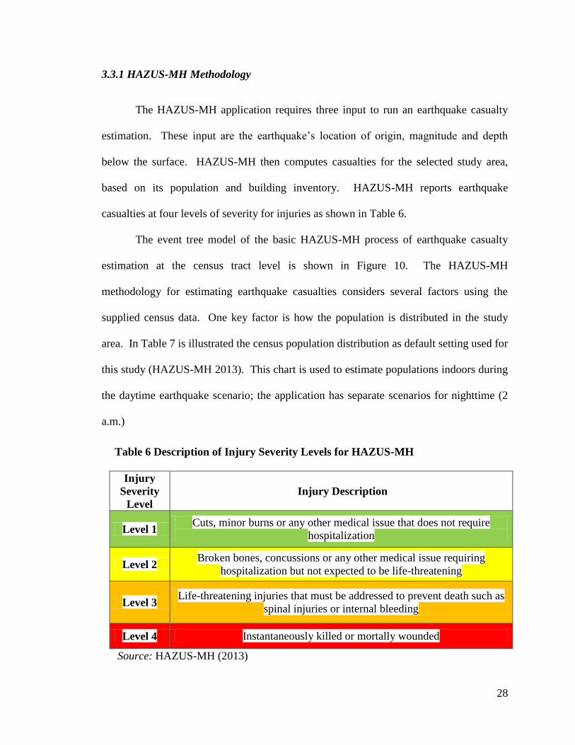
Table 6 Description of Injury Severity Levels for HAZUS-MH

Injury

Severity

Level

Injury Description

Level 1 Cuts, minor burns or any other medical issue that does not require

hospitalization

Level 2 Broken bones, concussions or any other medical issue requiring

hospitalization but not expected to be life-threatening

Level 3 Life-threatening injuries that must be addressed to prevent death such as

spinal injuries or internal bleeding

Level 4 Instantaneously killed or mortally wounded

Source: HAZUS-MH (2013)

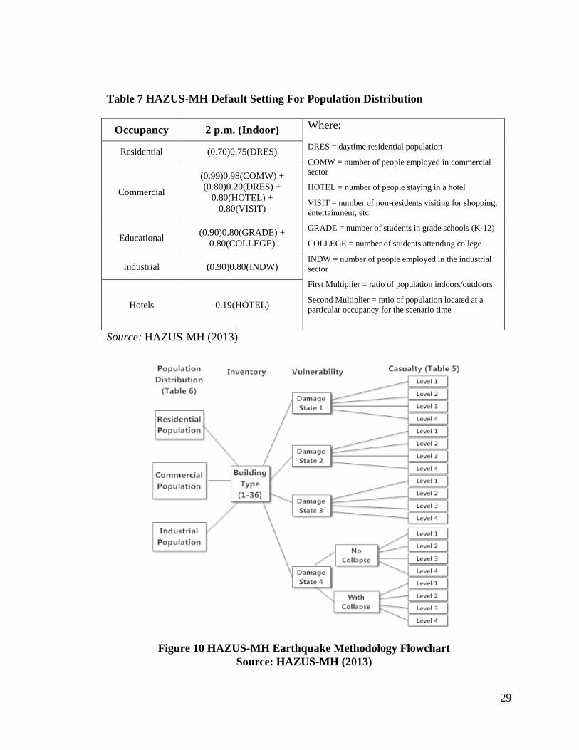
29

Figure 10 HAZUS-MH Earthquake Methodology Flowchart


Table 7 HAZUS-MH Default Setting For Population Distribution

Occupancy 2 p.m. (Indoor) Where:

DRES = daytime residential population

COMW = number of people employed in commercial

sector

HOTEL = number of people staying in a hotel

VISIT = number of non-residents visiting for shopping,

entertainment, etc.

GRADE = number of students in grade schools (K-12)

COLLEGE = number of students attending college

INDW = number of people employed in the industrial

sector

First Multiplier = ratio of population indoors/outdoors

Second Multiplier = ratio of population located at a

particular occupancy for the scenario time

Residential (0.70)0.75(DRES)

Commercial

(0.99)0.98(COMW) +

(0.80)0.20(DRES) +

0.80(HOTEL) +

0.80(VISIT)

Educational (0.90)0.80(GRADE) +

0.80(COLLEGE)

Industrial (0.90)0.80(INDW)

Hotels 0.19(HOTEL)


30

and commute time (5 p.m.). Using the right scenario is important as the population is

assumed not to be stationary over a 24-hour period. Another important assumption in

HAZUS-MH relates to the ratio of the population that would be located indoors or

outdoors during the earthquake in an attempt to better simulate a real-life scenario, thus

leading to more accurate casualty counts. For this study, only indoor casualties were

considered.

The other major input HAZUS-MH considers when estimating earthquake

casualties is the building inventory contained in the application. The HAZUS-MH

earthquake technical manual lists default casualty rates for 36 different building types for

five damage states: slight, moderate, extensive, complete (non-collapse) and complete

(collapse) (HAZUS-MH 2013). Each building type has a specific vulnerability to seismic

activity based on type of construction, building materials and number of stories. The

complete tables of these casualty rates by building type can be viewed in Appendices A

through E.

3.3.2 UDSCE Method at Census Tract Level

The UDSCE method was developed in an attempt to simplify the HAZUS-MH

method of estimating casualties in an urbanized area as the result of an earthquake

occurring during the day. The UDSCE new methodology is outlined in Figure 11. This

method allows for casualty estimations to be viewed at a census block level, improving

upon the limitation of HAZUS-MH results at the census tract level. The foundation of

the UDSCE method is the scoring process of three key building components: building

height, age and material. The total scores are then grouped according to the damage

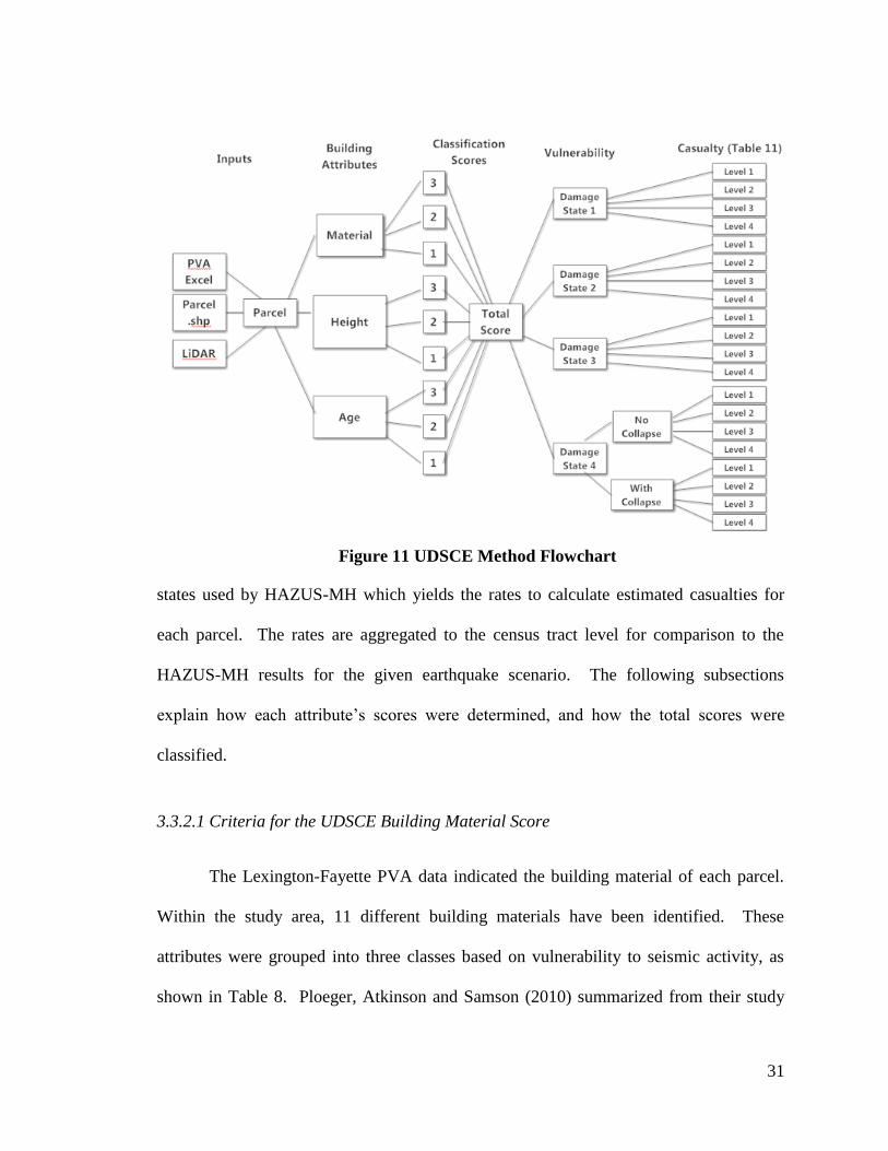
31

states used by HAZUS-MH which yields the rates to calculate estimated casualties for

each parcel. The rates are aggregated to the census tract level for comparison to the

HAZUS-MH results for the given earthquake scenario. The following subsections

explain how each attribute’s scores were determined, and how the total scores were

classified.

3.3.2.1 Criteria for the UDSCE Building Material Score

The Lexington-Fayette PVA data indicated the building material of each parcel.

Within the study area, 11 different building materials have been identified. These

attributes were grouped into three classes based on vulnerability to seismic activity, as

shown in Table 8. Ploeger, Atkinson and Samson (2010) summarized from their study

Figure 11 UDSCE Method Flowchart

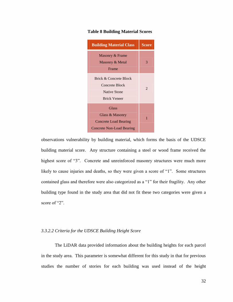
32

observations vulnerability by building material, which forms the basis of the UDSCE

building material score. Any structure containing a steel or wood frame received the

highest score of “3”. Concrete and unreinforced masonry structures were much more

likely to cause injuries and deaths, so they were given a score of “1”. Some structures

contained glass and therefore were also categorized as a “1” for their fragility. Any other

building type found in the study area that did not fit these two categories were given a

score of “2”.

3.3.2.2 Criteria for the UDSCE Building Height Score

The LiDAR data provided information about the building heights for each parcel

in the study area. This parameter is somewhat different for this study in that for previous

studies the number of stories for each building was used instead of the height

Table 8 Building Material Scores

Building Material Class Score

Masonry & Frame

Masonry & Metal

Frame

3

Brick & Concrete Block

Concrete Block

Native Stone

Brick Veneer

2

Glass

Glass & Masonry

Concrete Load Bearing

Concrete Non-Load Bearing

1

33

measurement. Güzey et. al. (2013) and Hashemi and Alisheikh (2011) each factored in

number of stories in their respective building vulnerability studies, with higher storied

buildings generally more likely to cause casualties in an earthquake as shown in Table 9.

The HAZUS-MH application in most cases allocate 10 or 12 feet per story in their

building classification methodology to determine the building’s approximate height. For

this study, each building up to 100 feet [1-8 stories] in height received a score of “3”,

buildings between 100 to 150 feet [9-12 stories] in height received a score of “2” and all

buildings taller than 150 feet [13 or more stories] in height received a score of “1”.

3.3.2.3 Criteria for the UDSCE Building Age Score

The age of the structures play a part in its vulnerability to earthquakes. The

HAZUS-MH application classifies structures by four different levels of code: high-code,

moderate code, low code, and pre-code (built before seismic standards). The year built is

a large factor in this designation, but to a smaller degree and so is the region of the

country the building is located (HAZUS-MH 2013). Putting the year built attribute from

the Lexington-Fayette PVA data into year ranges of vulnerability was done for this study

as summarized in Table 10. The lowest score of “1” was assigned to structures built

Table 9 Building Height Scores

Height Range Number

of Stories Score

Up to 100 feet 1-8 3

100-150 feet 9-12 2

Above 150 feet 13+ 1

34

before 1940, since no seismic codes existed before this date. For any structure built

between 1940 and 1979, a score of “2” was designated, and a score of “3” was assigned

to the buildings built in 1980 and later.

3.3.2.4 Criteria for the UDSCE Total Score

Each parcel’s score for building material, height and age was then added up for a

total score. The total score represented what damage state the structure would fall and to

which would be assigned the casualty rates among the four injury severity levels from the

Table 11 Total Score Ratings

Total

Score Damage State

8-9 Slight

6-7 Moderate

5 Extensive

4 Complete

(No Collapse)

3 Complete (Collapse)

Table 10 Building Age Scores

Year Built Range Score

1980 - Current 3

Between 1940-1979 2

Before 1940 1

35

correlating tables found in HAZUS-MH (HAZUS-MH 2013). The resulting total scores

are summarized in Table 11. Since the HAZUS-MH indoor casualty rate tables

(HAZUS-MH 2013) have listings for 36 different building types, the most common rates

found within each table were used for the UDSCE method. These rates are summarized

in Table 12. Two examples of the computed scores predicting vulnerability and

casualties can be seen in Table 13 and 14.

The ModelBuilder application in ArcGIS 10.2 was used to automate the process

of calculating all new fields for both the scores and the associated casualty rates. A

snapshot of the model can be viewed in Figure 12. The input StudyAreaParcels shapefile

has already been pre-processed with the addition of the three parameters identified to

predict vulnerability to seismic activity. By running this model, all necessary fields were

created and populated by the criteria described, then the parcel casualty rates were

aggregated.

Table 12 UDSCE Assigned Casualty Rates by Damage State

Total

Score Damage State

Casualties (%) % HAZUS-

MH Building

Types Use Level 1 Level 2 Level 3 Level 4

8-9 Slight .05 0 0 0 100

6-7 Moderate .20 .025 0 0 52.78

5 Extensive 1 .1 .001 .001 94.44

4 Complete

(No collapse) 5 1 .01 .01 94.44

3 Complete

(Collapse) 40 20 5 10 91.67

36

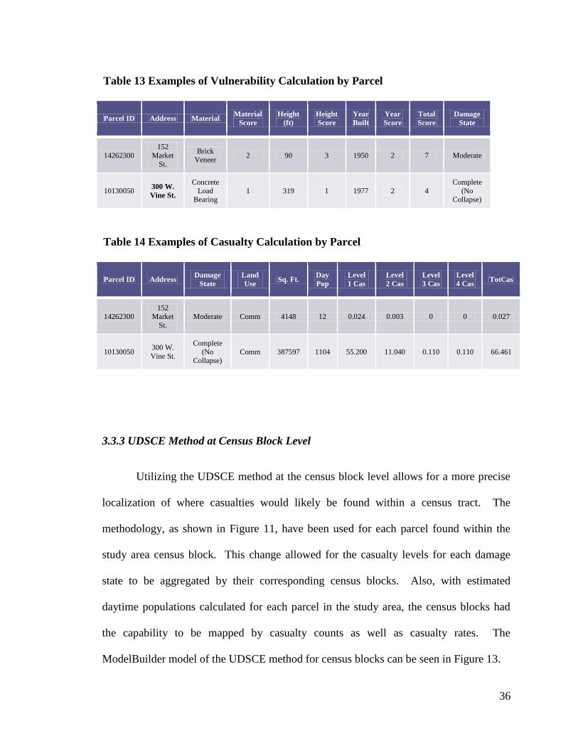
3.3.3 UDSCE Method at Census Block Level

Utilizing the UDSCE method at the census block level allows for a more precise

localization of where casualties would likely be found within a census tract. The

methodology, as shown in Figure 11, have been used for each parcel found within the

study area census block. This change allowed for the casualty levels for each damage

state to be aggregated by their corresponding census blocks. Also, with estimated

daytime populations calculated for each parcel in the study area, the census blocks had

the capability to be mapped by casualty counts as well as casualty rates. The

ModelBuilder model of the UDSCE method for census blocks can be seen in Figure 13.

Table 13 Examples of Vulnerability Calculation by Parcel

Parcel ID Address Material Material

Score

Height

(ft)

Height

Score

Year

Built

Year

Score

Total

Score

Damage

State

14262300

152

Market

St.

Brick Veneer

2 90 3 1950 2 7 Moderate

10130050 300 W.

Vine St.

Concrete

Load Bearing

1 319 1 1977 2 4

Complete

(No Collapse)

Table 14 Examples of Casualty Calculation by Parcel

Parcel ID Address Damage

State

Land

Use Sq. Ft.

Day

Pop

Level

1 Cas

Level

2 Cas

Level

3 Cas

Level

4 Cas TotCas

14262300

152

Market

St.

Moderate Comm 4148 12 0.024 0.003 0 0 0.027

10130050 300 W.

Vine St.

Complete

(No Collapse)

Comm 387597 1104 55.200 11.040 0.110 0.110 66.461

37

Figure 13 ModelBuilder Design of UDSCE Method by Census Block

Figure 12 ModelBuilder Design of UDSCE Method by Census Tract

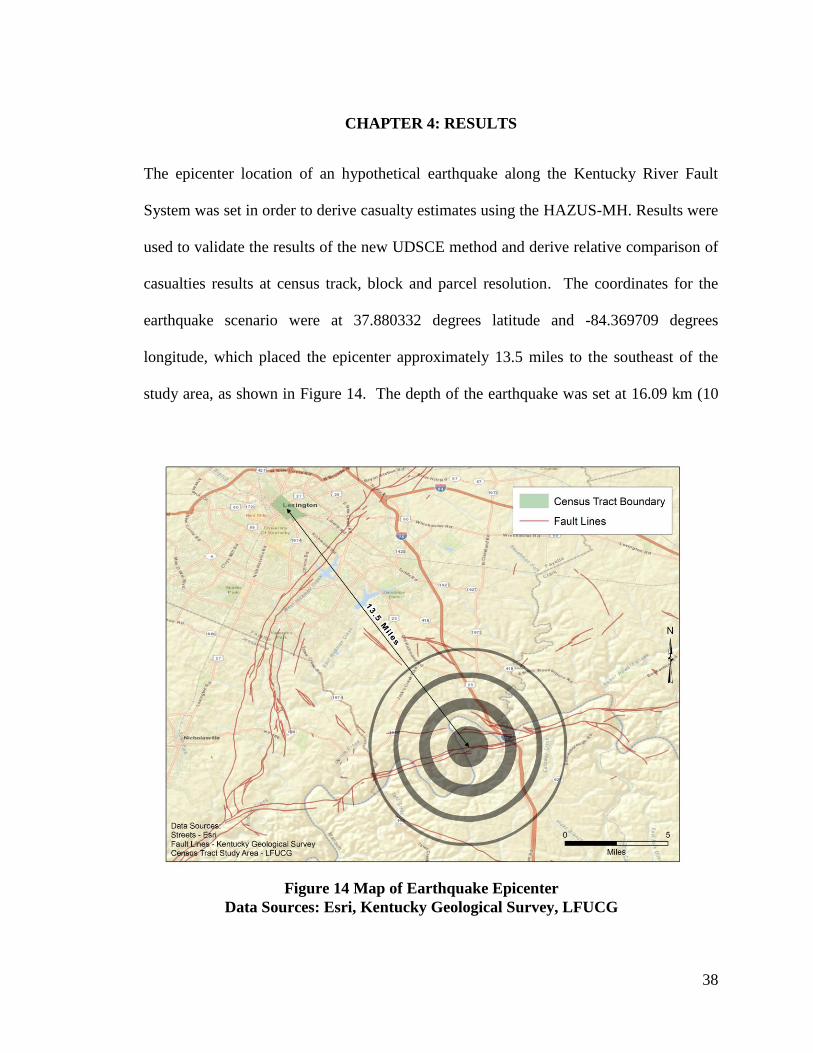
38

CHAPTER 4: RESULTS

The epicenter location of an hypothetical earthquake along the Kentucky River Fault

System was set in order to derive casualty estimates using the HAZUS-MH. Results were

used to validate the results of the new UDSCE method and derive relative comparison of

casualties results at census track, block and parcel resolution. The coordinates for the

earthquake scenario were at 37.880332 degrees latitude and -84.369709 degrees

longitude, which placed the epicenter approximately 13.5 miles to the southeast of the

study area, as shown in Figure 14. The depth of the earthquake was set at 16.09 km (10

Figure 14 Map of Earthquake Epicenter

Data Sources: Esri, Kentucky Geological Survey, LFUCG

39

miles) below the surface, based on historical earthquake records documented in the area

(Street 1982).

First the HAZUS-MH application was run with the determined epicenter input

under three magnitude scenarios: 5.5 (Moderate 5-5.9), 6.2 and 6.8 (Strong 6-6.9). The

classes are listed according to the Earthquake Magnitude Classes (UPSeis 2014). The

recorded earthquake effects for the used magnitudes are:

2.5 to 5.4 Often felt, but only causes minor damage

5.5 to 6.0 Slight damage to buildings and other structures

6.1 to 6.9 May cause a lot of damage in very populated areas

This was done to evaluate at what strength the relative runs with the UDSCE method

would best model the casualty counts at the census track level. Then the UDSCE model

was run, for the same scenario, at the census block level and parcel level to refine the

casualty estimates at higher resolution.

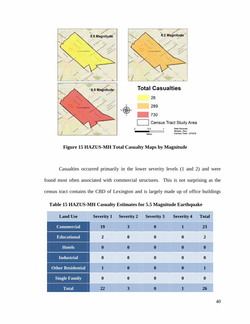
4.1 HAZUS-MH Results

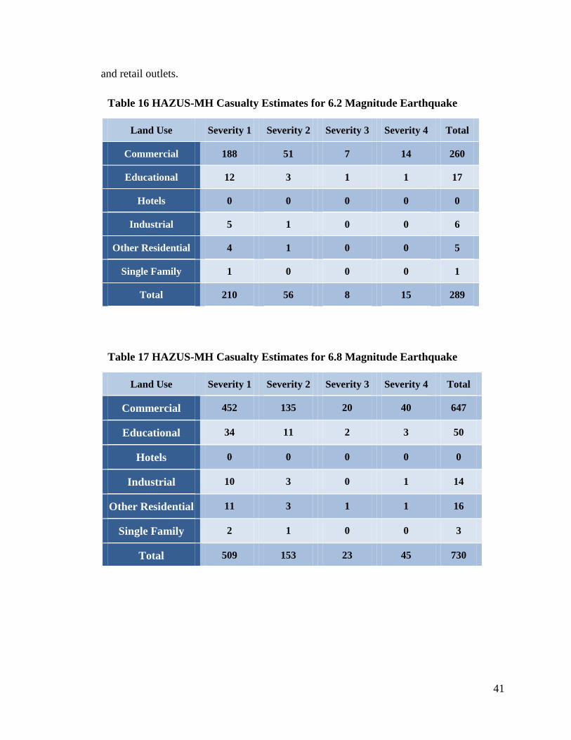
The results of the total casualty estimations from three separate magnitudes for

census tract #21067000100 can be seen in Figure 15. The complete breakdown for each

magnitude by severity level are summarized in Table 15, 16 and 17. These casualty

estimates represent the 2 p.m. (afternoon) scenario only for people located indoors.

Counts were broken down by the four severity levels as well as by building use. For the

5.5 magnitude scenario, the number of total injuries expected was 26, with one potential

death. A total of 289 casualties were predicted under the 6.2 magnitude scenario,

including 15 deaths. The 6.8 magnitude scenario calculated 730 casualties, of which 45

people lost their lives.

40

Casualties occurred primarily in the lower severity levels (1 and 2) and were

found most often associated with commercial structures. This is not surprising as the

census tract contains the CBD of Lexington and is largely made up of office buildings

Table 15 HAZUS-MH Casualty Estimates for 5.5 Magnitude Earthquake

Land Use Severity 1 Severity 2 Severity 3 Severity 4 Total

Commercial 19 3 0 1 23

Educational 2 0 0 0 2

Hotels 0 0 0 0 0

Industrial 0 0 0 0 0

Other Residential 1 0 0 0 1

Single Family 0 0 0 0 0

Total 22 3 0 1 26

Figure 15 HAZUS-MH Total Casualty Maps by Magnitude

41

and retail outlets.



Commercial 452 135 20 40 647


Hotels 0 0 0 0 0




Total 509 153 23 45 730



Commercial 188 51 7 14 260


Hotels 0 0 0 0 0




Total 210 56 8 15 289

42

4.2 UDSCE Method at Census Tract Level Results

The results of the UDSCE method for determining total casualties from

earthquakes are shown in Figure 16 while the complete breakdown by severity level is

shown in Table 18. It is important to note that the UDSCE method was not designed to

receive input of magnitude like HAZUS-MH but rather assigned casualty rates by

damage state (Section 3.3.2, Table 11). These results are representative of the census

block study area of parcels within the census tract, shown in Figure 9, rather than the

entire census tract used for the HAZUS-MH studies. This extent was determined by the

PVA spreadsheet of parcels covering only the entire census block study area. However,

Figure 16 UDSCE Method Total Casualties in Study Area Map

43

as noted in Section 3.2.1, 92.5 percent of the CBD commercial space from the census

tract is included in the census block study area, and the HAZUS-MH studies conducted

show that this is where most of the injuries would occur. A total of 371 injuries for the

census block study area were predicted under the UDSCE method, with the potential for

one fatality.

Just like in the HAZUS-MH studies, injuries were on the lower levels of severity

and most commonly associated with the CDB commercial structures. No injuries were

expected with hotels or single family residences, as people typically do not occupy them

during the early afternoon hours. Casualties from educational and industrial parcels were

not evident in this case as no parcels within the study area fit either of these criteria.

4.2.1 Validation of UDSCE Method

In comparison to the HAZUS-MH predictions, the UDSCE method suggests that

it is modeling earthquake casualties at multiple strengths based on the severity level. For

Table 18 UDSCE Method For Study Area Results


Commercial 303 57 1 1 362


Hotels 0 0 0 0 0




Total 310 59 1 1 371

44

total casualties, the UDSCE method has the closest ties to the 6.2 magnitude scenario

from HAZUS-MH, as seen in Table 19. In contrast, the Severity 3 and Severity 4 levels

of casualties predicted by the UDSCE method are much closer to the 5.5 magnitude

prediction generated by the HAZUS-MH method, in which these levels of injuries are

rare.

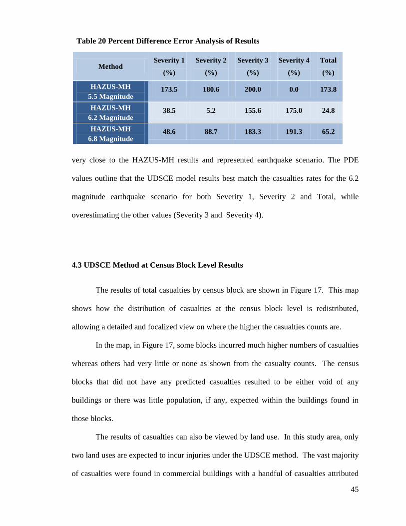
For a closer look at the differences in estimations between the three HAZUS-MH

models and the UDSCE model, the Percent Difference Error (PDE) analysis was used

(University of California, Davis 2014). This analysis can be used to compare model

values, in this case the HAZUS-MH results and the UDSCE method results. In equation

(1) the absolute value of the difference between the HAZUS-MH value (h) and the

UDSCE value (u) divided by their average is multiplied by 100:

(1)

where: h = the HAZUS-MH result; u = the UDSCE method result.

The results of the percent difference error analysis are summarized in Table 20. A

percentage difference error very close to zero means that the UDSCE model values are

Table 19 Comparison of HAZUS-MH and UDSCE Results

Method Severity 1 Severity 2 Severity 3 Severity 4 Total

HAZUS-MH

5.5 Magnitude 22 3 0 1 26

HAZUS-MH

6.2 Magnitude 210 56 8 15 289

HAZUS-MH

6.8 Magnitude 509 153 23 45 730

UDSCE Method 310 59 1 1 371

45

very close to the HAZUS-MH results and represented earthquake scenario. The PDE

values outline that the UDSCE model results best match the casualties rates for the 6.2

magnitude earthquake scenario for both Severity 1, Severity 2 and Total, while

overestimating the other values (Severity 3 and Severity 4).

4.3 UDSCE Method at Census Block Level Results

The results of total casualties by census block are shown in Figure 17. This map

shows how the distribution of casualties at the census block level is redistributed,

allowing a detailed and focalized view on where the higher the casualties counts are.

In the map, in Figure 17, some blocks incurred much higher numbers of casualties

whereas others had very little or none as shown from the casualty counts. The census

blocks that did not have any predicted casualties resulted to be either void of any

buildings or there was little population, if any, expected within the buildings found in

those blocks.

The results of casualties can also be viewed by land use. In this study area, only

two land uses are expected to incur injuries under the UDSCE method. The vast majority

of casualties were found in commercial buildings with a handful of casualties attributed

Table 20 Percent Difference Error Analysis of Results

Method Severity 1

(%)

Severity 2

(%)

Severity 3

(%)

Severity 4

(%)

Total

(%)

HAZUS-MH

5.5 Magnitude 173.5 180.6 200.0 0.0 173.8

HAZUS-MH

6.2 Magnitude 38.5 5.2 155.6 175.0 24.8

HAZUS-MH

6.8 Magnitude 48.6 88.7 183.3 191.3 65.2

46

Figure 18 Census Block Casualties By Land Use. Casualties in Commercial land

use estimated at 357, for Commercial & Residential at 14

Figure 17 Estimation of Casualties by Census Block

47

to residential. The results of the casualties by land use are shown in Figure 18. The

results from the UDSCE method at census block level are very promising and give a

better understanding of the casualties distribution which could be extremely helpful to

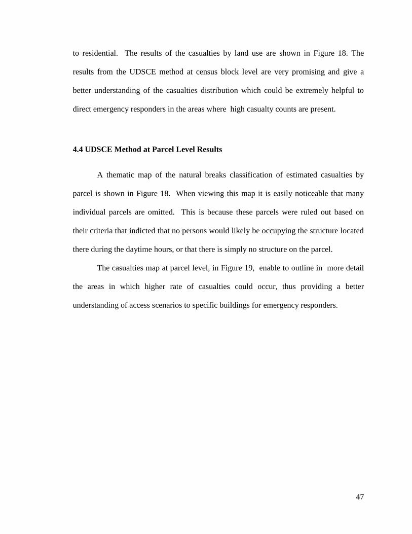
direct emergency responders in the areas where high casualty counts are present.

4.4 UDSCE Method at Parcel Level Results

A thematic map of the natural breaks classification of estimated casualties by

parcel is shown in Figure 18. When viewing this map it is easily noticeable that many

individual parcels are omitted. This is because these parcels were ruled out based on

their criteria that indicted that no persons would likely be occupying the structure located

there during the daytime hours, or that there is simply no structure on the parcel.

The casualties map at parcel level, in Figure 19, enable to outline in more detail

the areas in which higher rate of casualties could occur, thus providing a better

understanding of access scenarios to specific buildings for emergency responders.

48

Figure 19 Estimation of Casualties by Parcel

49

CHAPTER 5: CONCLUSIONS AND FUTURE WORK

Chapter 5 summarizes the conclusions and insights on possible future steps that could be

undertaken for the use and improvement of the new UDSCE method.

5.1 Conclusions

The HAZUS-MH application model earthquake casualties at the census tract

level, hence the UDSCE method was designed to identify potential casualties at a higher

resolution level in urbanized areas. The UDSCE method was validated with results from

three HAZUS-MH models, at three different magnitude scenarios, for the census tract

containing the CBD of Lexington, Kentucky. Casualties at higher resolution, in the

urbanized area, were then calculated using the UDSCE method at a census block level.

The validation process of the UDSCE method went well overall. By comparing

this method with three earthquake scenario models generated from HAZUS-MH, an

indication was given of an approximate earthquake strength that the UDSCE method best

models. The UDSCE method predicted 371 total casualties, putting it closer in line with

the “Strong” 6.2 magnitude HAZUS-MH scenario at 289 casualties. In general the

UDSCE method results overestimated casualties for Severity 1 and Severity 2 in a

“Strong” earthquake case scenario while the Severity 3 and Severity 4 levels are

underestimated, as evidenced by the Percent Difference Error analysis results in Table 17.

The change in study area from the HAZUS-MH models to the UDSCE method was not a

factor as the vast majority of casualties came from commercial buildings and 92.5 percent

50

of the commercial space within the HAZUS-MH census tract was located inside the

block group study area utilized by the UDSCE method. This was a good indicator that

the UDSCE method would be a competent alternative for earthquake casualty modeling

to HAZUS-MH.

Once the UDSCE method was validated, the next step was to group the casualty

count by census blocks for the high resolution analysis. This was done with the UDSCE

method analysis at census block and individual parcels level. The resulting maps, shown

in Figure 16, 17, and 18 (Section 4.3 and 4.4), outline how widely the injuries can vary

within the study area. Only a handful of census blocks and parcels contained the majority

of the total casualties, whereas many other blocks and parcels have shown very little or

no casualties. Casualties by land use were also analyzed and clearly outlined that high

casualties occurred in Commercial and Commercial & Residential land use categories,

while only nine people were hurt that were not in a commercial building.

5.2 Future Work

The results in this study have shown the capability to outline where injuries could

occur within the urbanized area at the block and parcels level, thus facilitating emergency

response in the case of a powerful earthquake taking place during the daytime hours.

However, improvements are possible and considerations for future work are discussed in

the following sections in regard to data use, flexibility of the UDSCE method, areal

constraints, population estimations and factors affecting the estimates.

51

5.2.1 Data Availability

The data used to develop the UDSCE method was derived from local sources.

These sources included the PVA spreadsheet data, local government parcel shapefiles and

LiDAR developed by a private business. The three primary parameters that made up the

new UDSCE method were easily available and provided the necessary detail that for a

solid model foundation, though improvements could be made especially when

considering building parameters.

The PVA data provided general building material attributes but were not nearly as

detailed as the building types that HAZUS-MH utilized. Better detail of construction of

the buildings, such as knowing whether structures are reinforced with stronger materials

on the inside, could enhance the scoring method and deliver better results.

Additional parameters should also be considered for future studies with the

UDSCE method. One parameter in particular that would add value is the soil makeup of

the study area. Soil type plays a part in determining the vulnerability of structures and

can vary even in an urbanized area (Ploeger, Atkinson and Samson 2010).

5.2.2 Flexibility of UDSCE Method

The UDSCE method is suited for a specific type of study area (urban with a large

commercial presence) and a specific time of day (in the middle of a day). This method

would not be helpful for a study area made up of mostly residential areas. Hopefully, any

future work done with this method would yield information that would help develop this

methodology to assess vulnerability and casualties in places like residential areas.

52

The UDSCE method was also developed in a way so that it can easily be

compared to the HAZUS-MH application, in accordance with earthquake hazard

standards, for verification. The UDSCE method did not take into consideration the input

that HAZUS-MH requires for its scenario such as epicenter coordinates, magnitude and

depth, therefore the only way to verify the findings is to conduct multiple HAZUS-MH

scenarios with different magnitudes and see how which one best resembled the UDSCE

results. Potentially the same earthquake input scenarios could be implemented in the

UDSCE method, however, more work must be done in this direction to allow users this

advanced flexibility.

5.2.3 Study Area Constraints

The CBD of Lexington, Kentucky was selected for the trial run of the UDSCE

method. This study area fit entirely within one census tract, which meant that there was

only one census tract to compare between the HAZUS-MH and the UDSCE results for

validation purposes, however, this could be a limitation in the validation process.

Selecting an urbanized area containing multiple census tracts would lead to multiple

comparison and increasing data would allow to refine indicators of the accuracy of the

UDSCE method depending on the complexity of the urban scenarios. Future development

of this method should consider analyzing data derived from multiple census tracts.

5.2.4 Population Estimations

Casualty estimations generated by the UDSCE method relied on a formula that

estimated what the population would be within all structures located in the selected study

53

area. Square footage and land use were the two factors that were used in this study.

Much more could be done to improve the accuracy of the population counts. For

example, occupancy rates of office buildings and apartment complexes would be good

information to know to improve upon the population estimation. Also, better knowledge

of commuting populations would help with the development of a better population

estimation formula.

5.2.5 Time Factors Affecting Estimates

Changes to the UDSCE method could help accurately predict casualties at other

times of the day. A nighttime scenario would shift the focus to residential areas for

assessing building vulnerability and calculating population for locating casualties.

Depending on the study area, building height may be less relevant and LiDAR data may

not be as useful for this purpose. However, LiDAR could be utilized for population

estimations, as explained with examples in Section 1.2.3 in this study. These

developments would open up the possibility to improving upon the HAZUS-MH method

of estimating earthquake casualties of census tracts of residential areas.

54

REFERENCES

Aydöner, C. and D. Maktav. April 2009. The role of the integration of remote sensing

and GIS in land use/land cover analysis after an earthquake. International

Journal of Remote Sensing 30(7): 1697-1717.

Barazzetti, L., M. A. Brovelli and L. Valentini. 2010. LiDAR digital building models

for true orthophoto generation. Applied Geomatics, 2(4): 187-196.

Campbell, J. B. and R. H. Wynne 2011. Introduction to Remote Sensing, Fifth Edition.

New York: The Guilford Press.

Central United States Earthquake Consortium (CUSEC). 2013. Central U.S. Earthquake

Consortium – CUSEC. http://www.cusec.org/ (last accessed 29 September 2013)

Dell’Acqua, F. and P. Gamba. October 2012. Remote sensing and earthquake damage

assessment: experiences, limits, and perspectives. Proceedings of the IEEE 100

(10): 2876-2890.

Dong, P., S. Ramesh, and A. Nepali. 10 November 2010. Evaluation of small-area

population estimation using LiDAR, Landsat TM and parcel data. International

Journal of Remote Sensing, 31(21): 5571-5586.

Esri. October 2008. Geographic information systems providing the platform for

comprehensive emergency management. http://www.esri.com/industries/public-

safety/~/media/Files/Pdfs/library/whitepapers/pdfs/gis-platform-emergency-

management.pdf (last accessed 4 February 2014).

Federal Emergency Management Agency (FEMA). 2014. Hazus.

http://www.fema.gov/hazus (last accessed 4 February 2014).

Geiβ, C. and H. Taubenböck. August 2013. Remote sensing contributing to assess

earthquake risk: from a literature review towards a roadmap. Natural Hazards

68(1): 7-48.

Gillespie, T. W., J. Chu, E. Frankenburg, and D. Thomas. 2007. Assessment and

prediction of natural hazards from satellite imagery. Progress in Physical

Geography 31(5): 459-470.

Güzey, Ö, E. Aksoy, A. C. Gel, Ö. Anil, N. Gültekin and S. O. Akbas. 2013. An inter-

disciplinary approach for earthquake vulnerability assessment in urban areas: A

case study of Central District, Yalova. Regional Studies Association, Annual

European Conference, University of Tampere, Tampere, Finland.

55

Hashemi, M. and A. A. Alisheikh. 2011. A GIS-based earthquake damage assessment

and settlement methodology. Soil Dynamics and Earthquake Engineering, 31:

1607-1617.

HAZUS-MH. 2012. Version 2.1. Federal Emergency Management Agency. Washington,

D.C., United States of America.

Kentucky Geological Survey (KGS). 2013. http://www.uky.edu/KGS/ (last accessed 10

November 2013).

Kirscher, C. A., R. V. Whitman and W. T. Holmes. May 2006. HAZUS Earthquake

Loss Estimation Methods. Natural Hazards Review 7: 45-59.

Lexington/Fayette Urban County Government (LFUCG). 2013. Geographic Information

Systems. http://www.lexingtonky.gov/index.aspx?page=416 (last accessed 29

September 2013).

Lexington-Fayette Property Valuation Administrator (PVA) Office. 2013. http://fayette-

pva.com (last accessed 15 March 2014)

Liu, J. G., P. J. Mason, E. Yu, M. C. Wu, C. Tang, R. Huang, and H. Liu. February 2012.

GIS modeling of earthquake damage zones using satellite remote sensing and

DEM data. Geomorphology 139-140: 518-535.

Mauk, F. J., D. Christensen, and S. Henry. February 1982. The Sharpsburg, Kentucky

earthquake 27 July 1980: main shock parameters and isoseismal maps. Bulletin of

the Seismological Society of America 72(1): 221-236.

Miller, N. 2012. Estimating Office Space per Worker. University of San Diego.

http://www.sandiego.edu/pipeline/documents/EstimatingOfficeSpaceRequirement

sMay12012.pdf (last accessed 13 November 2013).

Moffatt, S. F. and T. J. Cova. 2010. Parcel-scale Earthquake Loss Estimation with

HAZUS: A Case Study in Salt Lake County, Utah. Cartography and Geographic

Information Science 37(1): 17-29.

National Earthquake Hazards Reduction Program (NEHRP). 2014. http://www.nehrp.gov/ (last accessed 4 February 2014).Neighbors, C. J., E. S.

Cochran, Y. Caras and G. R. Noriega. 2013. Sensitivity Analysis of FEMA

HAZUS Earthquake Model: Case Study from King County, Washington. Natural

Hazards Review 14(2): 134-146.

Ploeger, S. K., G. M. Atkinson and C. Samson. 2010. Applying the HAZUS-MH

software tool to assess seismic risk in downtown Ottawa, Canada. Natural

Hazards 53: 1-20.

56

Qiu, F., H. Sridharan, and Y. Chun. July 2010. Spatial autoregressive model for

population estimation at the census block level using LIDAR-derived building

volume information. Cartography and Geographic Information Science, 37(3):

239-257.

Remo, J. W. F. and N. Pinter. 2012. HAZUS-MH earthquake modeling in the central

USA. Natural Hazards 62: 1055-1081.

Sahar, L., S. Muthukumar, and S. P. French. September 2010. Using aerial imagery and

GIS in automated building footprint extraction and shape recognition for

earthquake risk assessment of urban inventories. Transactions on Geoscience and

Remote Sensing 48 (9): 3511-3520.

Sampath, A. and J. Shan. 2007. Building boundary tracing and regularization from

airborne LIDAR point clouds. Photogrammetry Engineering Remote Sensing,

73(7): 805–812.

Show Me Net. 2014. New Madrid Seismic Zone.

http://www.showme.net/~fkeller/quake/comments.htm (last accessed 16 June

2014)

Silván-Cárdenas, J. L., L. Wang, P. Rogerson, C. Wu, T. Feng, and B. D. Kamphaus.

2010. Assessing fine-spatial-resolution remote sensing for small-area population

estimation. International Journal of Remote Sensing, 31(21): 5605-5634.

Street, R. August 1982. Ground motion values obtained from the 27 July 1980

Sharpsburg, Kentucky earthquake. Bulletin of the Seismological Society of

America 72(4): 1295-1307.

The Business Journals. 18 April 2008. Earthquakes Shake Louisville Area.

http://www.bizjournals.com/louisville/stories/2008/04/14/daily36.html (last

accessed 5 March 2014).

United States Census Bureau. 2013. http://www.census.gov (last accessed 20 December

2013).

United States Geological Survey (USGS). 2014. Building Safer Structures.

http://earthquake.usgs.gov/learn/publications/saferstructures (last accessed 2

February 2014).

University of California, Davis. 2014.

http://www.physics.ucdavis.edu/Classes/Physics9Lab/Phy9BLab/9ASupplements.

pdf (last accessed 6 June 2014).

UPSeis. 2014. http://www.geo.mtu.edu/UPSeis/magnitude.html (last accessed 4 June

2014).

57

Vanarsdale, R. November 1986. Quaternary displacement on faults within the Kentucky

River fault system of east-central Kentucky. Geological Society of America

Bulletin 97: 1382-1392.

58

APPENDIX A: Indoor Casualty Rates by Model Building Type for Slight Structural

Damage

# Building Type

(Appendix F)

Severity 1

(%)

Severity 2

(%)

Severity 3

(%)

Severity 4

(%)

1 W1 0.05 0 0 0

2 W2 0.05 0 0 0

3 S1L 0.05 0 0 0

4 S1M 0.05 0 0 0

5 S1H 0.05 0 0 0

6 S2L 0.05 0 0 0

7 S2M 0.05 0 0 0

8 S2H 0.05 0 0 0

9 S3 0.05 0 0 0

10 S4L 0.05 0 0 0

11 S4M 0.05 0 0 0

12 S4H 0.05 0 0 0

13 S5L 0.05 0 0 0

14 S5M 0.05 0 0 0

15 S5H 0.05 0 0 0

16 C1L 0.05 0 0 0

17 C1M 0.05 0 0 0

18 C1H 0.05 0 0 0

19 C2L 0.05 0 0 0

20 C2M 0.05 0 0 0

21 C2H 0.05 0 0 0

22 C3L 0.05 0 0 0

23 C3M 0.05 0 0 0

24 C3H 0.05 0 0 0

25 PC1 0.05 0 0 0

26 PC2L 0.05 0 0 0

27 PC2M 0.05 0 0 0

28 PC2H 0.05 0 0 0

29 RM1L 0.05 0 0 0

30 RM1M 0.05 0 0 0

31 RM2L 0.05 0 0 0

32 RM2M 0.05 0 0 0

33 RM2H 0.05 0 0 0

34 URML 0.05 0 0 0

35 URMM 0.05 0 0 0

36 MH 0.05 0 0 0


59

APPENDIX B: Indoor Casualty Rates by Model Building Type for Moderate

Structural Damage

# Building Type

(Appendix F)

Severity 1

(%)

Severity 2

(%)

Severity 3

(%)

Severity 4

(%)

1 W1 0.25 0.030 0 0

2 W2 0.20 0.025 0 0

3 S1L 0.20 0.025 0 0

4 S1M 0.20 0.025 0 0

5 S1H 0.20 0.025 0 0

6 S2L 0.20 0.025 0 0

7 S2M 0.20 0.025 0 0

8 S2H 0.20 0.025 0 0

9 S3 0.20 0.025 0 0

10 S4L 0.25 0.030 0 0

11 S4M 0.25 0.030 0 0

12 S4H 0.25 0.030 0 0

13 S5L 0.20 0.025 0 0

14 S5M 0.20 0.025 0 0

15 S5H 0.20 0.025 0 0

16 C1L 0.25 0.030 0 0

17 C1M 0.25 0.030 0 0

18 C1H 0.25 0.030 0 0

19 C2L 0.25 0.030 0 0

20 C2M 0.25 0.030 0 0

21 C2H 0.25 0.030 0 0

22 C3L 0.20 0.025 0 0

23 C3M 0.20 0.025 0 0

24 C3H 0.20 0.025 0 0

25 PC1 0.25 0.030 0 0

26 PC2L 0.25 0.030 0 0

27 PC2M 0.25 0.030 0 0

28 PC2H 0.25 0.030 0 0

29 RM1L 0.20 0.025 0 0

30 RM1M 0.20 0.025 0 0

31 RM2L 0.20 0.025 0 0

32 RM2M 0.20 0.025 0 0

33 RM2H 0.20 0.025 0 0

34 URML 0.35 0.400 0.001 0.001

35 URMM 0.35 0.400 0.001 0.001

36 MH 0.25 0.030 0 0


60

APPENDIX C: Indoor Casualty Rates by Model Building Type for Extensive

Structural Damage

# Building Type

(Appendix F)

Severity 1

(%)

Severity 2

(%)

Severity 3

(%)

Severity 4

(%)

1 W1 1 .1 0.001 0.001

2 W2 1 .1 0.001 0.001

3 S1L 1 .1 0.001 0.001

4 S1M 1 .1 0.001 0.001

5 S1H 1 .1 0.001 0.001

6 S2L 1 .1 0.001 0.001

7 S2M 1 .1 0.001 0.001

8 S2H 1 .1 0.001 0.001

9 S3 1 .1 0.001 0.001

10 S4L 1 .1 0.001 0.001

11 S4M 1 .1 0.001 0.001

12 S4H 1 .1 0.001 0.001

13 S5L 1 .1 0.001 0.001

14 S5M 1 .1 0.001 0.001

15 S5H 1 .1 0.001 0.001

16 C1L 1 .1 0.001 0.001

17 C1M 1 .1 0.001 0.001

18 C1H 1 .1 0.001 0.001

19 C2L 1 .1 0.001 0.001

20 C2M 1 .1 0.001 0.001

21 C2H 1 .1 0.001 0.001

22 C3L 1 .1 0.001 0.001

23 C3M 1 .1 0.001 0.001

24 C3H 1 .1 0.001 0.001

25 PC1 1 .1 0.001 0.001

26 PC2L 1 .1 0.001 0.001

27 PC2M 1 .1 0.001 0.001

28 PC2H 1 .1 0.001 0.001

29 RM1L 1 .1 0.001 0.001

30 RM1M 1 .1 0.001 0.001

31 RM2L 1 .1 0.001 0.001

32 RM2M 1 .1 0.001 0.001

33 RM2H 1 .1 0.001 0.001

34 URML 2 .2 0.002 0.002

35 URMM 2 .2 0.002 0.002

36 MH 1 .1 0.001 0.001


61

APPENDIX D: Indoor Casualty Rates by Model Building Type for Complete

Structural Damage (No Collapse)

# Building Type

(Appendix F)

Severity 1

(%)

Severity 2

(%)

Severity 3

(%)

Severity 4

(%)

1 W1 5 1 0.01 0.01

2 W2 5 1 0.01 0.01

3 S1L 5 1 0.01 0.01

4 S1M 5 1 0.01 0.01

5 S1H 5 1 0.01 0.01

6 S2L 5 1 0.01 0.01

7 S2M 5 1 0.01 0.01

8 S2H 5 1 0.01 0.01

9 S3 5 1 0.01 0.01

10 S4L 5 1 0.01 0.01

11 S4M 5 1 0.01 0.01

12 S4H 5 1 0.01 0.01

13 S5L 5 1 0.01 0.01

14 S5M 5 1 0.01 0.01

15 S5H 5 1 0.01 0.01

16 C1L 5 1 0.01 0.01

17 C1M 5 1 0.01 0.01

18 C1H 5 1 0.01 0.01

19 C2L 5 1 0.01 0.01

20 C2M 5 1 0.01 0.01

21 C2H 5 1 0.01 0.01

22 C3L 5 1 0.01 0.01

23 C3M 5 1 0.01 0.01

24 C3H 5 1 0.01 0.01

25 PC1 5 1 0.01 0.01

26 PC2L 5 1 0.01 0.01

27 PC2M 5 1 0.01 0.01

28 PC2H 5 1 0.01 0.01

29 RM1L 5 1 0.01 0.01

30 RM1M 5 1 0.01 0.01

31 RM2L 5 1 0.01 0.01

32 RM2M 5 1 0.01 0.01

33 RM2H 5 1 0.01 0.01

34 URML 10 2 0.02 0.02

35 URMM 10 2 0.02 0.02

36 MH 5 1 0.01 0.01


62

APPENDIX E: Indoor Casualty Rates by Model Building Type for Complete

Structural Damage (With Collapse)

# Building Type

(Appendix F)

Severity 1

(%)

Severity 2

(%)

Severity 3

(%)

Severity 4

(%)

1 W1 40 20 3 5

2 W2 40 20 5 10

3 S1L 40 20 5 10

4 S1M 40 20 5 10

5 S1H 40 20 5 10

6 S2L 40 20 5 10

7 S2M 40 20 5 10

8 S2H 40 20 5 10

9 S3 40 20 3 5

10 S4L 40 20 5 10

11 S4M 40 20 5 10

12 S4H 40 20 5 10

13 S5L 40 20 5 10

14 S5M 40 20 5 10

15 S5H 40 20 5 10

16 C1L 40 20 5 10

17 C1M 40 20 5 10

18 C1H 40 20 5 10

19 C2L 40 20 5 10

20 C2M 40 20 5 10

21 C2H 40 20 5 10

22 C3L 40 20 5 10

23 C3M 40 20 5 10

24 C3H 40 20 5 10

25 PC1 40 20 5 10

26 PC2L 40 20 5 10

27 PC2M 40 20 5 10

28 PC2H 40 20 5 10

29 RM1L 40 20 5 10

30 RM1M 40 20 5 10

31 RM2L 40 20 5 10

32 RM2M 40 20 5 10

33 RM2H 40 20 5 10

34 URML 40 20 5 10

35 URMM 40 20 5 10

36 MH 40 20 3 5


63

APPENDIX F: Explanation of Building Types

# Building

Type Description

1 W1 Wood Light Frame >5,000 sq. ft.

2 W2 Wood Commercial and Industrial <5,000 sq. ft.

3 S1L Steel Moment Frame Low-Rise (1-3 stories)

4 S1M Steel Moment Frame Mid-Rise (4-7 stories)

5 S1H Steel Moment Frame High-Rise (8 + stories)

6 S2L Steel Braced Frame Low-Rise (1-3 stories)

7 S2M Steel Braced Frame Mid-Rise (4-7 stories)

8 S2H Steel Braced Frame High-Rise (8 + stories)

9 S3 Steel Light Frame

10 S4L Steel Frame with Cast-in-Place Concrete Shear Walls Low-Rise

(1-3 stories)

11 S4M Steel Frame with Cast-in-Place Concrete Shear Walls Mid-Rise

(4-7 stories)

12 S4H Steel Frame with Cast-in-Place Concrete Shear Walls High-Rise

(8 + stories)

13 S5L Steel Frame with Unreinforced Masonry Infill Walls Low-Rise

(1-3 stories)

14 S5M Steel Frame with Unreinforced Masonry Infill Walls Mid-Rise

(4-7 stories)

15 S5H Steel Frame with Unreinforced Masonry Infill Walls High-Rise

(8 + stories)

16 C1L Concrete Moment Frame Low-Rise (1-3 stories)

17 C1M Concrete Moment Frame Mid-Rise (4-7 stories)

18 C1H Concrete Moment Frame High-Rise (8 + stories)

19 C2L Concrete Shear Wall Low-Rise (1-3 stories)

20 C2M Concrete Shear Wall Mid-Rise (4-7 stories)

21 C2H Concrete Shear Wall High-Rise (8 + stories)

22 C3L Concrete Frame with Unreinforced Masonry Infill Walls Low-Rise

(1-3 stories)

23 C3M Concrete Frame with Unreinforced Masonry Infill Walls Mid-Rise

(4-7 stories)

24 C3H Concrete Frame with Unreinforced Masonry Infill Walls High-Rise

(8 + stories)

25 PC1 Precast Concrete Tilt-up Walls

26 PC2L Precast Concrete Frames with Concrete Shear Walls Low-Rise

(1-3 stories)

27 PC2M Precast Concrete Frames with Concrete Shear Walls Mid-Rise

(4-7 stories)

28 PC2H Precast Concrete Frames with Concrete Shear Walls High-Rise

64

(8 + stories)

29 RM1L Reinforced Masonry Bearing Walls with Wood or Metal Deck

Diaphragms Low-Rise (1-3 stories)

30 RM1M Reinforced Masonry Bearing Walls with Wood or Metal Deck

Diaphragms Mid-Rise (4 + stories)

31 RM2L Reinforced Masonry Bearing Walls with Precast Concrete Diaphragms

Low-Rise (1-3 stories)

32 RM2M Reinforced Masonry Bearing Walls with Precast Concrete Diaphragms

Mid-Rise (4-7 stories)

33 RM2H Reinforced Masonry Bearing Walls with Precast Concrete Diaphragms

High-Rise (8 + stories)

34 URML Unreinforced Masonry Bearing Walls Low-Rise (1-2 stories)

35 URMM Unreinforced Masonry Bearing Walls Mid-Rise (3 + stories)

36 MH Mobile Homes


analyzing earthquake casualty risk at … · 2014-07-18 · analyzing earthquake casualty risk at...

Documents