1

Analyzing policy impacts and international price shocks: Alternative Computable General Equilibrium (CGE) models

for an aid-dependent less-industrialized country

Lorenzo Giovanni Bellù April 2011

Abstract This paper addresses the issue of analyzing how complex socio-economic systems are hit by and adjust to external shocks and polices. In the first section the focus is put on the structure of a socio-economic system, and on "entry points" of different types of shocks and policies. Subsequently, alternative general equilibrium models are analyzed, with a focus on macro-economic and factor markets closures, highlighting how different closures imply different assumptions related to the way the economic system and related adjustments work. To test how different ways of designing general equilibrium models may influence actual decision making in less industrialized economies, a one-sector, two-household, two-factor general equilibrium model is designed and calibrated on an “archetypical” Social Accounting Matrix of a less industrialized, aid-dependent country. Alternative macro-economic and factor market closures are tested focusing on the mechanisms through which the economic system adjusts to external shocks such as import price upward shifts. Conclusions highlight that: 1) different ways of modelling the economic systems lead to significantly different impacts of the same simulated external shock on import prices; 2) the results are particularly sensitive to the level of the elasticities of substitution of domestic goods with domestic ones; and 3) in aid-dependent economies, characterized by an high foreign dependency ratio of the government budget and an high level of foreign borrowing due to the external trade deficit, trade shocks affecting the real exchange rate largely affect the system and the welfare of households. This due to the fact that they affect the real exchange rate, which in turn shift the value of both foreign savings in domestic currency in the Savings-Investment balance and the foreign transfers in domestic currency in the government balance. These shifts require the adjustments of the S-I and government balances through the adjustments of all the other endogenous variables entering these balances. This particularly applies when investment demand and government consumption are exogenous and kept fixed to the pre-shock level. Table of contents 1 Introduction ........................................................................................................................ 22 Analyzing economic systems and their adjustments to policies and shocks ...................... 2

2.1 Structure of a socio-economic system. ....................................................................... 32.2 Identifying entry points of policies and shocks into an economic system. ................ 42.3 Modelling impacts of policy measures and shocks .................................................... 7

3 Alternative computable general equilibrium models (CGE) .............................................. 84 Applying general equilibrium models for actual decision making .................................. 19

4.1 A one-sector, two-household, two-factor general equilibrium model ..................... 204.2 An “archetypical” SAM of an aid-dependent less industrialized country. .............. 254.3 Alternative macro-economic and factor market closures ......................................... 27

5 Some policy implications ................................................................................................. 366 Conclusions ...................................................................................................................... 377 References ........................................................................................................................ 38

2

1 Introduction This paper proposes an analysis of the way different external shocks or policy measures affect an economic system, with the aim of identifying analytical implications relevant for policy making. Even economic policies, aimed at affecting specific segments of the economic system may have significant spill-overs and macro-economic impacts through the channels mutually linking production activities, factor markets, households, the government and the “rest of the world”. For this reason CGE models are widespread tools to simulate ex-ante the possible impacts of various policy options. However, the results of the simulations have to be interpreted in the light of the macro-economic and factor-related assumptions undertaken. Various authors carried out comparative analyses of alternative macro and factor market closures, such as Sen (1963), Pasinetti (1972), Taylor –Lysy (1978), Rattso (1982), De Melo, Robinson (1989). However, the results of the alternative closure rules and the extent of their mutual discrepancies depend also on the structure of the economic system under investigation. For socio-economic development policy making it is important to better understand the extent to which the different closures affect the results of CGE models when they are applied to less industrialized countries with specific features. After section 2, illustrating how policies and external shocks affect a complex socio-economic system, detailed discussion of selected alternative macro-economic and factor market closure is carried out in section 3. To investigate the extent to which the different macro and factor market closures provide different results, a simple one-sector, two-factor, two-household general equilibrium model is designed and presented in section 4.1. The SAM of a “paradigmatic” aid-dependent oil-importing less-industrialized country adopted to calibrate the CGE model is presented in section 4.2. Some tests with alternative closure rules carried out simulating the impacts of an international import price shock are presented and discussed in section 4.3. Some implications for policy making emerging from the different ways of modelling socio-economic systems are presented, together with concluding remarks at the end of the paper.

2 Analyzing economic systems and their adjustments to policies and shocks Identifying and describing the fundamental relationships among the constituting elements of an economic system is a pre-requisite for understanding how this system evolves and adjusts to stimuli coming from external shocks or policy measures. Any kind of economic analysis, to generate new knowledge and to be functional to decision making processes, should consider the causal links between a shock, whether policy-induced or generated by other external factors, and the modifications likely to occur in the economic system. External shocks and policy measures affect a socio-economic system by modifying the behaviour of economic agents, whether they are producers, consumers or suppliers of factor services, such as workers, investors or renters. To understand how external shocks and policy measures modify the behaviour and relations among different economic agents within an economic system and to obtain analytical results relevant for decision making in policy processes, it is worth: 1) exploring the structure of a socio-economic system; 2) identifying “entry points” of the different policy measures and other shocks into the economic system; and 3) modelling the economic system and the causal relationships linking policies-shock to impacts.

3

2.1 Structure of a socio-economic system. A socio-economic system can be seen as a set of elements, mutually linked by means of physical flows (flows of goods and services) and countervailing flows of payments, flowing in the opposite direction. The System of National Accounts of the United Nations (SNA UN)1

1. Commodities: Goods and services produced, purchased, sold and consumed by various economic agents within an economic system. Commodities are exchanges on commodity markets where supply and demand meets;

, a standard approach for national accounts adopted by almost all countries, identifies some basic elements of a socio-economic system. For each of these, inflows and outflows of payments (income and expenditure, respectively) are recorded on two-side balancing accounts for each period (usually a year). These elements comprise:

2. Activities: Economic sectors (industries) which produce commodities by using other commodities (intermediate consumption), factor services;

3. Factors: Services provided by economic agents for activities such as labour, land and capital services; remunerated by payments such as wages, rents, interests, profits.

4. Institutions: Economic agents such as households, enterprises and the government. They are classified as “private” institutions (households, enterprises) and “public” (the government). Private institutions provide factor services to activities, and to other institutions, by supplying them on factor markets. Private institutions are remunerated with payments for factor services, which constitute their income. Institutions consume final consumption goods and services, whose payments constitute their expenditure. The part of income not spent is saved. The government, as a public institution, collects taxes from other institutions (direct taxes) and activities (indirect taxes). It transfers money to other institutions and activities (public transfers) and directly provides selected services (defence, justice etc.).

5. Savings-Investment. This account keeps track of the savings (income not spent) of the institutions and of the demand for investment goods. This account acts as a peculiar “institution” which receives the income not spent from the other institutions (their savings) and allocates it to purchase investment goods. In addition, this account may receive savings from the Rest of the World (RoW) or may “invest” lending money to the RoW.

6. “Rest of the World” (RoW). This is an account that keeps track of the transactions between the domestic agents and the economic agents outside the economic system, i.e. the rest of the world. The inflows of this account comprise payments for imports; payments for services provided by foreign agents to the national economy; such as immigrants into the country, expatriation of earnings of foreign corporations and transfers from domestic institutions to foreign institutions. The outflows comprise payments for exports, remittances of emigrants and transfers from foreign to domestic institutions2

1United Nations, Statistical Division (1993): System of National Accounts.

.

http://unstats.un.org/unsd/sna1993/toctop.asp 2 In the SNA, the RoW and S-I accounts are used to square up the two-side, balanced accounts system. The balance of the RoW account in a given period represents the deficit or surplus of the RoW towards the country in that period. If it shows a deficit, this implies a surplus in the current external balance of the country, i.e. the RoW received more money from the country than it paid. The balance is then transferred to the Savings-Investment account as an “investment of the country” abroad. In this case, the country is a net lender to the RoW. If the RoW account shows a surplus, this implies that the RoW received less money from the country than it paid out. The balance is then transferred to the Savings-Investment account as a “foreign savings”. In this case, the country is a net borrower from the RoW. Note that being this a two-side, balanced accounting system, once all

4

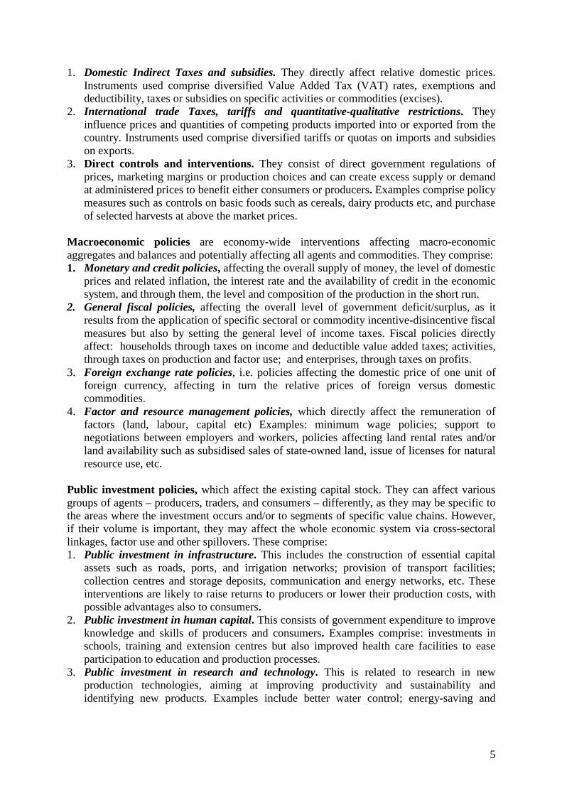
These elements and the flows of income interlinking them are represented in Figure 1. Figure 1: Elements of a socio-economic system and their mutual linkages

Source: Freely adapted from Round (2003)

2.2 Identifying entry points of policies and shocks into an economic system. Development policies affect an economic system through the use of policy instruments, i.e. variables or sets of variables directly under control of decision makers. Also non policy-led external shocks, such as shifts of exogenous international prices or exogenous technological changes, enter the economic system through the direct modification of selected variables affecting the behaviour of economic agents. Different policy measures mostly adopted to stimulate development or react to external shocks such as a) price policies; b) macro-economic policies; c) public investment policies, are normally implemented through the use of different policy instruments, i.e. socio-economic variables directly or indirectly under the control of the policy makers. Price policies, i.e. policies aimed at directly shifting the relative prices of one good or a set of goods with respect to the others are generally implemented through:

the other accounts balance, the deficit-surplus of the RoW account exactly matches the surplus-deficit of the S-I account.

Links within a socio-economic system: the circular flow of income

Activities Households

Current external balance (+/-)

Indirect taxes Savings

Savings-Invest.

Value Added

Factor Markets

Internat. Transfers

Enterprises

Domestic Transfers

Exports

Taxes

Government

Inputs

Commodity Markets

Outputs

Imports Rest of the

World

Final consumption

Profits

Investment

5

1. Domestic Indirect Taxes and subsidies. They directly affect relative domestic prices. Instruments used comprise diversified Value Added Tax (VAT) rates, exemptions and deductibility, taxes or subsidies on specific activities or commodities (excises).

2. International trade Taxes, tariffs and quantitative-qualitative restrictions. They influence prices and quantities of competing products imported into or exported from the country. Instruments used comprise diversified tariffs or quotas on imports and subsidies on exports.

3. Direct controls and interventions. They consist of direct government regulations of prices, marketing margins or production choices and can create excess supply or demand at administered prices to benefit either consumers or producers. Examples comprise policy measures such as controls on basic foods such as cereals, dairy products etc, and purchase of selected harvests at above the market prices.

Macroeconomic policies are economy-wide interventions affecting macro-economic aggregates and balances and potentially affecting all agents and commodities. They comprise: 1. Monetary and credit policies, affecting the overall supply of money, the level of domestic

prices and related inflation, the interest rate and the availability of credit in the economic system, and through them, the level and composition of the production in the short run.

2. General fiscal policies, affecting the overall level of government deficit/surplus, as it results from the application of specific sectoral or commodity incentive-disincentive fiscal measures but also by setting the general level of income taxes. Fiscal policies directly affect: households through taxes on income and deductible value added taxes; activities, through taxes on production and factor use; and enterprises, through taxes on profits.

3. Foreign exchange rate policies, i.e. policies affecting the domestic price of one unit of foreign currency, affecting in turn the relative prices of foreign versus domestic commodities.

4. Factor and resource management policies, which directly affect the remuneration of factors (land, labour, capital etc) Examples: minimum wage policies; support to negotiations between employers and workers, policies affecting land rental rates and/or land availability such as subsidised sales of state-owned land, issue of licenses for natural resource use, etc.

Public investment policies, which affect the existing capital stock. They can affect various groups of agents – producers, traders, and consumers – differently, as they may be specific to the areas where the investment occurs and/or to segments of specific value chains. However, if their volume is important, they may affect the whole economic system via cross-sectoral linkages, factor use and other spillovers. These comprise: 1. Public investment in infrastructure. This includes the construction of essential capital

assets such as roads, ports, and irrigation networks; provision of transport facilities; collection centres and storage deposits, communication and energy networks, etc. These interventions are likely to raise returns to producers or lower their production costs, with possible advantages also to consumers.

2. Public investment in human capital. This consists of government expenditure to improve knowledge and skills of producers and consumers. Examples comprise: investments in schools, training and extension centres but also improved health care facilities to ease participation to education and production processes.

3. Public investment in research and technology. This is related to research in new production technologies, aiming at improving productivity and sustainability and identifying new products. Examples include better water control; energy-saving and

6

carbon-reducing production processes, development of drugs, development and provision of technological breakthroughs, etc.

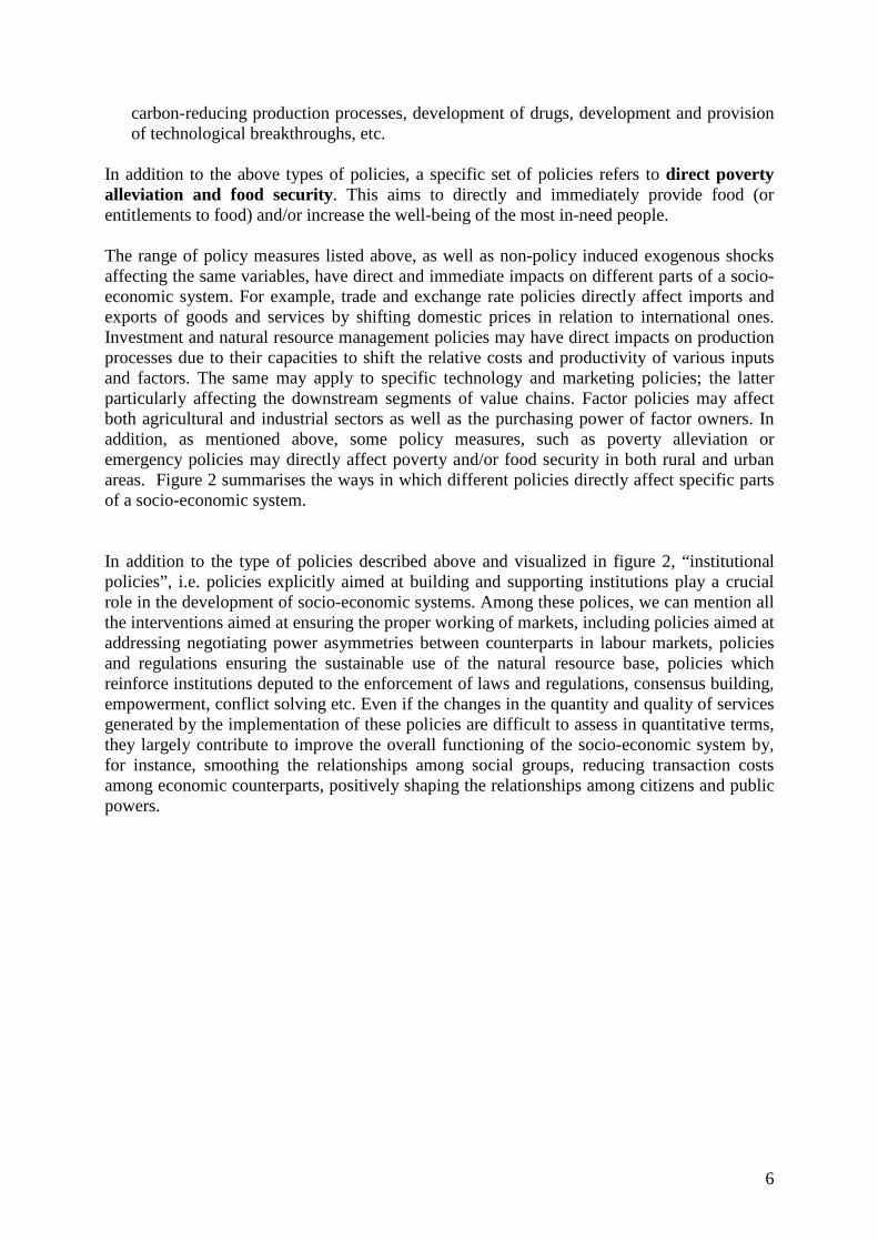
In addition to the above types of policies, a specific set of policies refers to direct poverty alleviation and food security. This aims to directly and immediately provide food (or entitlements to food) and/or increase the well-being of the most in-need people. The range of policy measures listed above, as well as non-policy induced exogenous shocks affecting the same variables, have direct and immediate impacts on different parts of a socio-economic system. For example, trade and exchange rate policies directly affect imports and exports of goods and services by shifting domestic prices in relation to international ones. Investment and natural resource management policies may have direct impacts on production processes due to their capacities to shift the relative costs and productivity of various inputs and factors. The same may apply to specific technology and marketing policies; the latter particularly affecting the downstream segments of value chains. Factor policies may affect both agricultural and industrial sectors as well as the purchasing power of factor owners. In addition, as mentioned above, some policy measures, such as poverty alleviation or emergency policies may directly affect poverty and/or food security in both rural and urban areas. Figure 2 summarises the ways in which different policies directly affect specific parts of a socio-economic system. In addition to the type of policies described above and visualized in figure 2, “institutional policies”, i.e. policies explicitly aimed at building and supporting institutions play a crucial role in the development of socio-economic systems. Among these polices, we can mention all the interventions aimed at ensuring the proper working of markets, including policies aimed at addressing negotiating power asymmetries between counterparts in labour markets, policies and regulations ensuring the sustainable use of the natural resource base, policies which reinforce institutions deputed to the enforcement of laws and regulations, consensus building, empowerment, conflict solving etc. Even if the changes in the quantity and quality of services generated by the implementation of these policies are difficult to assess in quantitative terms, they largely contribute to improve the overall functioning of the socio-economic system by, for instance, smoothing the relationships among social groups, reducing transaction costs among economic counterparts, positively shaping the relationships among citizens and public powers.

7

Figure 2: Different types of policies-shocks and their entry points in the socio-economic system.

However, in addition to direct affects, the circular flow of payments linking the different elements of a system, gives rise to cross-sectoral and inter-institutional effects, i.e. to the activation of other parts of the economic system due to changes in one part. For example, increased household incomes may activate the demand of industrial goods, which in turn may activate the demand of industrial inputs and factors. This generates employment, increases the household income and further increases the demand of goods, thus increasing again incomes. In addition, investment may accelerate these effects by enhancing, period after period, the stock of capital and the efficiency of production and distribution processes.

2.3 Modelling impacts of policy measures and shocks Mathematical models can be used to quantify policy and shock impacts as long as they embody the essential features of economic systems and allow tracing the causal relationships linking exogenous changes to relevant socio-economic variables. This holds also for general equilibrium models, which are systems of simultaneous equations describing the essential

Activities Households

Current external balance (+/-)

Indirect taxes Savings

Savings-Invest.

Value Added

Factor Markets

Internat. Transfers

Enterprises

Domestic Transfers

Exports

Taxes

Government

Inputs

Commodity Markets

Outputs

Imports Rest of the

World

Final consumption

Profits

Investment

Trade and exchange rate policies-shocks

Factor and resource

policies-shocks

Poverty - food security policies-

shocks

Public Investment

polices-shocks

Fiscal policies-shocks

Monetary policies-shocks

Domestic Price policies- shocks

Technology and marketing

policies-shocks

8

elements of an economic system and related mutual linkages. Policy and shock impacts result by a counterfactual analysis, i.e. the comparison of the solutions of the model with and without the policy or shock3

. Values of relevant endogenous variables, i.e. variables whose values are determined by the solution of the equations, calculated “at the benchmark”, i.e. in a situation of reference, are compared with those calculated when relevant policy or other exogenous shocks are introduced by modifying selected exogenous variables (parameters). The difference or the percentage change of the endogenous variables or related indicators provides information on the impacts of the shocks on the economic system.

However, results of impact analyses depend, in addition to the type and magnitude of the exogenous shocks introduced into the model, by the way the economic system is modelled. More specifically, results are particularly sensitive to the assumptions regarding the so-called macro-economic and factor-markets closures, i.e. the way the equilibria of macro-economic balances such as the government budget, the saving-investment account and the current external current account, as well as the equilibria of the factor markets are achieved after the shock. Indeed, different assumptions regarding the above-mentioned balances reflect completely different visions on how the economic system adjusts to external shocks. In the following sections this issue will be addressed by exploring selected alternative approaches for modelling macro-economic balances and the equilibrium of factor markets in a general equilibrium context. Applications to an “archetypical” less industrialized country will allow us to illustrate the extent to which different modelling choices affect model results and, by way of consequence, policy decisions.

3 Alternative computable general equilibrium models (CGE) The concept of general equilibrium of an economic system dates back to Walras (1874)4, who highlighted how given a set of interrelated markets where supply and demand of different commodities meet under free competition, it is possible to determine a set of prices which implies the equilibrium of all the markets, and where each price matches the cost of production of each commodity. In more recent times Arrow and Debreu (1954)5, Debreu (1959)6 and others formalized this concept to allow its application to real economies. Selected authors, pioneered the application of general equilibrium models to actual economic issues such as Chenery and Uzawa (1958) to economic development, Johansen (1960) to economic growth, Harberger (1962) to corporate income taxes7. Showen and Walley (1972, 1974) extended the use of general equilibrium models to capital income and commodity taxes8

3 On the use of counterfactual analysis in policy decision making see e.g. Bellù L.G., Pansini R.V. (2009): Quantitative Socio-Economic Policy Impact Analysis: A Methodological Introduction. EASYPol series n.235.

.

www.fao.org/easypol Food and Agriculture Organization of U.N -Rome. 4 Walras, L. (1874) Éléments d’économie politique pure, ou théorie de la richesse sociale (Elements of pure economics, or theory of social wealth.) Lausanne, L. Borbax ed. 5 Arrow, K and Debreu, G. (1954). Existence of a Competitive Equilibrium for a Competitive Economy. Econometrica 22 (3): 265-290 6 Debreu, G. (1959) Theory of value: an axiomatic analysis of economic equilibrium. New York, Wiley 7 Chenery, H.B. and Uzawa H. (1958) Non-linear Programming in Economic development. In Arrow,K. Hurwicz, L. an Uzawa H. (eds) Studies in linear and on-linear programming, Palo Alto CA. Stanord University press. Harberger, A, (1962) The incidence of corporate income tax. Journal of political economy. 70: 215-240 8 Showen, J.B. and Whalley J. (1972) A general equilibrium calculation of the effects of differential taxation on income from capital . Journal of public economics 1, 281-322. Showen, J.B. and Whalley J. (1974) A proof of the existence o a general equilibrium with ad valorem commodity taxes. Journal of economic theory 8, 1-25.

9

Application to real cases has also been permitted by the works of various mathematical economists, such as Scarf, (1960, 1967), Merrill (1972), Van de Laan and Talman (1979), who worked out methods to actually compute vectors of equilibrium prices. A comparative review with illustrations of these methods can be found in Showen and Walley (1992)9

.

Since then, countless applications of general equilibrium models have been carried out to simulate ex ante the impacts of different policies and different types of models emerged according to various criteria such as: the specific purposes of the analysis, the different theoretical underpinnings specifically related to the causality links assumed to prevail in the economic system, their level of aggregation, the sources of statistical data utilized, the importance assigned to spatial factors, the time span covered etc. However, despite these multiple differences, following Willenbockel (1994)10 two major families of CGEs can be identified, according to their conceptual and operational roots: 1) CGEs rooted on the tradition of applied neoclassical welfare analysis; and 2) CGE rooted in the tradition quantitative development planning. Within the first category fit all the models adhering to the so called “Neo-Walrasian” paradigm. This category is traced back to the mentioned work of Harberger (1962) and includes the work of various authors such as Scarf, Showen and Whalley. Studies in this tradition assume that all the agents supplying and/or demanding factors and goods perform according to an optimizing behaviour, there is homogeneity of degree zero in prices and incomes, and there exist an appropriate set of prices for goods and factors which clear all the markets. The typical use of models following this approach is to carry out ex-ante comparative static analysis of policy impacts. Appropriate sets of clearing prices are identified at the benchmark (i.e. in the scenario without any policy change) and under the various scenarios reflecting the simulated policy changes. In the second category, named “Less-orthodox CGEs” Willenbockel fits the works which to a lesser or greater extent relax the strict Walrasian framework by introducing non-Walrasian elements such as nominal price rigidities, unbalanced government budgets in equilibrium, nominal exchange rates etc. This category hosts the pioneer contributions of Johansen (1960), a large number of CGE models designed for less-industrialized countries, but also large-scale multipurpose models such as the ORANI model of Australia by Dixon et al (1982), the Michigan model of world trade by Deardoff and Stern (1986)11

9 Scarf, H.E. (1960). Some examples of global instability of the competitive equilibrium. International economic review, 1, 157-172.

. In addition, this category hosts the contributions of the so called “macro-structuralists”, such as Lance Taylor (1990), who see themselves more in the tradition of Keynes, Kalecki and Kaldor rather than Walras, arrow and Debreu, and emphasize how the causation links in a CGE run from the macro-economic equilibrating

Scarf, H.E. (1967). The approximation of fixed points of a continuous mapping. SIAM. Journal of applied mathematics. 15, 1328-43. Merril, O.H. (1972). Applications and extension of an algorithm that computes fixed points of certain uppersemi-continuous point to set mapping. Department of Industrial Engineering, University of Michigan. Van der Laan, and G., Talman, A. J (1979). A restart algorithm for computing fixed point without an extra-dimension. Mathematical programming 17, 74-84. Showen, B.J., Walley, J. (1992) Applying general equilibrium. Cambridge surveys of economic literature, Cambridge University Press. 10 Willenbockel D. (1994) Applied general equilibrium modelling: Imperfect competition and European integration. Wiley. 11 Dixon, P.B, Parmenter, B.R., Sutton, J. and Vincent ,D.P. (1982). ORANI A multisectoral model of Australian economy. North Holland, Amsterdam. Deardorf A.V. and tern R.M. (1986). The Michigan model of world production and trade: theory and applications. Cambridge. MIT press. Taylor L. (1990). Structuralist CGE models, in Taylor L. (ed) ; Socially relevant Policy Analysis: Structural comptable general equilibrium models for developing world . Cambridge (MA): MIT press pp. 1-70.

10

mechanisms to the micro-economic distributional implications, i.e. the macro-closures chosen substantially influence the outcomes of the models. Missaglia (2011)12

He highlights how, despite the strikingly similar formal structure, expressed by means of a “complementarity” problem, i.e. a set of non-linear weak inequalities, the four models imply profoundly different visions about the way an economic system works. He argues that the intrinsic difference between a neoclassical and a Keynesian model is not the allowance for unemployment of the latter, which can also be included in the former. The actual difference consists in the fact that or the neo-classical model the “Say’s law” holds, while it does not for the Keynesian model. In other words, the “aggregated demand may never be deficient” as the supply “automatically” generates it. Unemployment, if present, is essentially generated within the labour market by some labour markets imperfections. Instead, in the Keynesian world, factor unemployment is essentially generated by the lack of effective demand. “Bastard Keynesian” models, are such that they work as a Keynesian model, through the working of the Keynesian multiplier, as an expansion of the autonomous demand, e.g. investment, generates an expansion of the labour demand and a contraction of unemployment. This happens until the full employment is reached. Beyond this point, these models work as neo-classical models, where the increase of investment occurs only at the expenses of consumption. Structuralist post Keynesian models, according to Missaglia, are essentially based on four assumptions: 1) in the short run there are almost no possibilities to substitute among factors; Leontief production functions are the only meaningful representations of the technology. 2) Income distribution is not determined by factors’ productivity but by social and institutional aspects. 3) Some markets are not competitive and agents are price-makers (e.g. mark-up pricing). 4) The Say’s law does not apply and aggregate demand matters to determine the level of output, factor use and welfare.

provides important hints to interpret the various strands of theoretical and applied CGE literature. Even if he does not provide a systematic clustering of the contributions in this domain, discusses in a formalized comparative way the salient features of: 1) Neo-classical models; 2) “Bastard Keynesian” models; and 3) Structuralist, post-Keynesian models; and 4) Stock-flow consistent post-keynesian models.

Stock-flow consistent post-keynesian models depict more realistic features of actual economic systems by explicitly introducing money (cash) as an asset. Cash, generated by the government to finance its deficit is held by the households as an asset at the beginning of each period. Cash is used, together with part of the income generated in the period to purchase goods and services. This Allows breaking the link between consumption-investment in one period and income generation in the same period. Also Thissen (1998)13

, among others, attempts a classification of CGEs. He substantially adheres to the classification provided by Willenbockel, but put more emphasis on the different macro-economic closures, that, in line with Lance Taylor, imply substantially different ways of conceiving the causal relationships in the economic system and essentially determine the quantitative results of the models.

12 Missaglia M. (2011). Neoclassical and Keynesian macro-models: Thinking about the special case. University

of Pavia,(It). MIMEO 13 Thissen M. (1998): A classification of empirical CGE modelling, p.9. SOM Research Report 99C01,

University of Groningen, The Netherlands.

11

The issue of macro-economic and factor-market closures in general equilibrium models was firstly addressed by Sen (1963)14

ws

. With a simple five-equation model, namely: 1) a production function (homogeneous of degree 1, output X as a function of labour L and capital stock K), 2) a wage function (wage w equal to marginal productivity of labour), 3) a “zero-extra-profit” function (total wages and profits π absorb all the product, .4) a saving-investment balance (savings determined by different propensities to save of recipients of wages w.r.t. recipients of profits πs ), and 5) an investment equation setting an exogenous investment level

*II = ), he highlighted that in general, it is not possible to determine an equilibrium solution if one wants to simultaneously achieve full employment of factors (as reflected by adding equations 6 and 7 to the system). This is due to the fact that only six variables are left to play with (namely X, π, w, I, L, K) for satisfying seven equations (see also Rattsø 1982)15

. The system s represented as follows:

),( LKXX = (1)

LXw∂∂

= (2)

wLX += π (3) wLssI w+= ππ (4)

*II = (5) *LL = (6)

*KK = (7) Sen himself, on the basis of existing literature, outlined four possible ways forward, which reflect different visions on how an economic system adjusts to exogenous shocks: 1. The “Neo-classical system” (closure). In this model, equation (5) is dropped, leaving the real investment to be “savings-driven” (equation 4). This model solves quite easily by replacing available factor endowments (equations 6 and 7) into the production function (equation 1) which determines the physical output X16

. The wage w is also determined by means of the equation (2), based on the position reached on the production function when fully employing the factor endowments. Once X and w are determined, and given L, π is worked out thanks to equation (3). Subsequently, by means of equation (4), savings are determined. Finally, even if it is not explicitly modelled, it is assumed that there is some mechanism bringing savings and investment in equilibrium, such as the interest rate, which is assumed to be positively linked to savings and negatively linked to investment.

14 Sen, A. (1963): “Neo-classical and neo-Keynesian theories of distribution” Economic Record, March 1963, pp 53-64.This simplified one-commody tmodel is in real terms, i.e. the price of the commodity X is set to 1. w is expressed as the quantity of commodity X per unit of labour. 15 We follow here the structure of the system with seven equations and six variables, as proposed in Rattsø J (1982). “Different Macroclosures of the original Johansen model and their impact on policy evaluation”. Journal of policy modelling 4(1): 85-87, rather than the one originally proposed by Sen of five equations (1 to 5) and four variables, where equations 6 and 7 are reported only in the text of the article but not included in the system. 16 An alternative “neoclassical” closure for an open-economy model is proposed in: Taylor L. And Lysy F.J (1979): Vanishing Income redistributions: Keynesian clues about model surprises in the short run. Journal of development economics, 6, (1979) 11-29, North Holland., where L is endogenously determined due to the fact factor prices are determined on the basis of international prices and existing technology, assuming that value added and intermediate (imported) inputs combine in fixed proportions.

12

2. The “Post-Keynesian system” (closure), or “Kaldorian” closure, from Kaldor (1955)17

wss >π

. Equation 2 is dropped, so that the real wage is no longer forced to reflect the marginal productivity of labour. In addition, the saving rate of profits is assumed to be higher than the saving rate of wages: . Assume for example an increase in investments, due e.g. to increased expectations about future profitability18. According to Robinson (1989)19

and Sen himself, this model adjusts through an income distribution mechanism, which allows reaching the Savings-Investment balance by altering the share of product allocated to profits. This is apparent when working out the share of profits in the total product, as expressed by Kaldor, starting from the above equations. First, note that the product allocated to wages wL in equation 4 can be expressed as the total product X minus the quantity of product allocated to profits:

)( π−= XwL (8)

Replacing the (8) into the (4) yields:

)( πππ −+= XssI w (4a)

which can be expressed as:

πππ ww sXssI −+=

)( ww ssXsI −+= ππ

Working out the profits, leads to: XsIss ww −=− )( ππ

)()( w

w

w ssXs

ssI

−−

−=

ππ

π (9)

Dividing by X leads to the share of profits on total product:

)()( w

w

w sss

XssI

X −−

−=

ππ

π (10)

The (10) is the “Post-Keynesian” (Kaldorian) equation for the profit share (see also Pasinetti, 1962)20

17 Kaldor N. (1955): “Alternative theories of distribution”. The review of economic studies. Pp 83-100.

.

18 In the Keynesian world, profitability expectations are among the driving forces of investments. 19 Robinson S. (1989) Multisectoral models, (chapter 18) in Handbook of development economics, Elsevier 20 Pasinetti L.(1962): Rate of profits and income distribution in relation to the rate of economic growth. The review of economic studies, vol. XXXIX n.4, Oct 1962 pp.267-279. Pasinetti associated specific saving rates not to the sources of income (profits and wages) as done by Kaldor, but to the social classes (workers and capitalists). He observed that, as the model envisages savings of the workers, the workers will necessarily receive a share of profits for their savings by lending them to capitalists at an interest rate i. By introducing the

13

Note that, as in this specification of the “Kaldorian” framework there is full employment of factors, i.e. equations (6) and (7) hold, given the technology, i.e. equation (1), also the output X is determined at the level:

*)*,(* LKXX = (1a) Assume that for I = I*, through the solution of the system of equations above it is possible to define equilibrium profits *π . In equilibrium, as the saving shares are given, this implies that there will be a corresponding income distribution given by:

)(*)(*

**

w

w

w sss

XssI

X −−

−=

ππ

π (10a)

Assume now that investments shift from *I to:

III ∆+= *** (5a)

As the output is fixed (given the technology and factor endowments), the economic system will adjust through a shift of product from consumption to investment, or, analogously, from consumption to savings. Given that saving rates are fixed, this can happen only by means of a shift of income between wages and profits, so that, thanks to the (10a), a new profit-product

ratio ***

Xπ will be determined:

)(*)(*

***

w

w

w sss

XssII

X −−

−∆+

=ππ

π (10b)

Developing the (10b) leads to:

*)()(*)(*

***

XssI

sss

XssI

X ww

w

w −∆

+−

−−

=πππ

π , (10c)

i.e., after substituting the (10a) in the (10c), leads to:

*)(**

***

XssI

XX w−∆

+=π

ππ , (10d)

Or also:

Iss w

∆−

=−)(

1***π

ππ

Calling πππ ∆=− ***

Leads to:

Iss w

∆−

=∆)(

1

π

π (11)

profits of the workers and assuming that in the long run the interest rate equals the profit rate, he worked out a

simplified expression for the profit share: Xs

IX π

π=

14

The (11) can be considered the multiplier of profits in the Kaldorian framework (with full employment).

The adjustments to a shock in a component of the aggregated demand in an actual economic system which presents the stylized features above, following Thissen (1998)21, if nominal wages are fixed for some institutional reasons, may occur through the increase of the general level of prices. This increase is due to the pressure on the demand side, which cannot be satisfied, given the full employment of factors. This leads to a reduction of the real wages and a related upward shift of profits, which in turn generates additional savings to compensate for the increase in investments22

.

3. The “Johansen” system (closure). In the Johansen approach23

, the equation (4) is dropped. At a first sight, it may appear that the Saving-Investment balance is dropped. In actual facts, equation (4) can be re-written introducing one more equation (4c) and one more variable (S) in the system as:

wLssS w+= ππ (4b) IS = (4c)

What is dropped is the (4b), i.e. the equality between savings and “voluntary” savings based on incomes. This implies that there may be in the system other sources of (positive or negative) savings, e.g. the government, so that equation (4b) can be re-written as:

GSAVwLssS w ++= ππ (4d) where GSAV is the new endogenous variable which completes the savings account. Note that the system has now eight variables (X, π, w, I, L, K, S, GSAV) and eight equations, notably:

),( LKXX = (1)

LXw∂∂

= (2)

wLX += π (3) IS = (4c)

GSAVwLssS w ++= ππ (4d) *II = (5) *LL = (6)

*KK = (7)

21 Thissen M. (1998): A classification of empirical CGE modelling, p.9. SOM Research Report 99C01, University of Groningen, The Netherlands. 22 Note that it is assumed here that, for some institutional reasons the employment supply does not drop as a consequence of a reduction of real wages, thus allowing the system to keep the same level of output X*. 23 Firstly introduced by Johansen, Leif (1960): “A multi-sectoral Study of economic growth”. Amsterdam, North-Holland (2nd enlarged edition, 1974). An early review and discussion of alternative macro-economic closures is also found in Rattso, J (1982): “different Macroclosures of the Original Johansen Model and Their Impact on Policy Evaluation”. Journal of Policy Modelling 4(1) p.85-97.

15

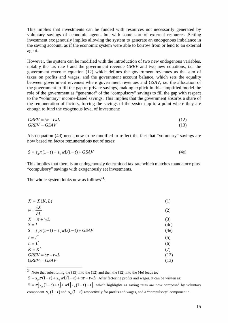
This implies that investments can be funded with resources not necessarily generated by voluntary savings of economic agents but with some sort of external resources. Setting investment exogenously implies allowing the system to generate an endogenous imbalance in the saving account, as if the economic system were able to borrow from or lend to an external agent. However, the system can be modified with the introduction of two new endogenous variables, notably the tax rate t and the government revenue GREV and two new equations, i.e. the government revenue equation (12) which defines the government revenues as the sum of taxes on profits and wages, and the government account balance, which sets the equality between government revenues where government revenues and GSAV, i.e. the allocation of the government to fill the gap of private savings, making explicit in this simplified model the role of the government as “generator” of the “compulsory” savings to fill the gap with respect to the “voluntary” income-based savings. This implies that the government absorbs a share of the remuneration of factors, forcing the savings of the system up to a point where they are enough to fund the exogenous level of investment:

twLtGREV += π (12) GSAVGREV = (13)

Also equation (4d) needs now to be modified to reflect the fact that “voluntary” savings are now based on factor remunerations net of taxes:

GSAVtwLstsS w +−+−= )1()1(ππ (4e) This implies that there is an endogenously determined tax rate which matches mandatory plus “compulsory” savings with exogenously set investments. The whole system looks now as follows24

:

),( LKXX = (1)

LXw∂∂

= (2)

wLX += π (3) IS = (4c)

GSAVtwLstsS w +−+−= )1()1(ππ (4e) *II = (5) *LL = (6)

*KK = (7) twLtGREV += π (12)

GSAVGREV = (13) 24 Note that substituting the (13) into the (12) and then the (12) into the (4e) leads to:

twLttwLstsS w ++−+−= πππ )1()1( . After factoring profits and wages, it can be written as:

[ ] [ ]ttswLttsS w +−++−= )1()1(ππ , which highlights as saving rates are now composed by voluntary

component )1( ts −π and )1( tsw − respectively for profits and wages, and a “compulsory” component t.

16

Note that here, π and wL represent now gross profits and wages. If we assume an external upward shift on the investment demand as illustrated for the case of the “post-keynesian” (Kaldorian) model, the “Johansen” system adjusts by: 1) maintaining the output level as determined by the full employment of factor endowments

(equations 1, 5 and 6); 2) setting the gross remuneration of factors as per equations (3) and (4c) 3) assuming that the government adjusts the tax rates (and related spending) in such a way

of generating enough savings (positive or negative) to compensate for the exogenous shock on investments;

4) Shifts in the tax rates adjust disposable incomes in such a way that the private consumption of goods reduces bring in equilibrium the commodity market, allowing for increased investment demand.

4. The “Keynesian” system (closure). In general terms, the Keynesian approach to economic development in setting the level of production gives prominence to the role of the “effective demand” (Keynes J.M.,1936)25

, rather than to the role of fully-employed factor endowments. Full employment will be reached only if the demand for investment equals the excess supply left after satisfying the demand for private consumption when all the labour is fully employed. This is a special case that can only exist “by accident or design”, as, in all the other cases, the level of (expected) effective demand will not be such to induce entrepreneurs to employ all the available labour. This conceptual framework justifies dropping equation (6) from the above system of equations, allowing the actual level of employment to be endogenously determined. However the system has now more endogenous variables than equations, In addition the equilibrium between investment and savings is no longer achieved by means of an endogenous tax rate, as in the Johansen system, but by shifts in real income which alter the volume of savings. Equation (6) can therefore be replaced by equation (14) which determines tax rate. Therefore, the whole system, which presents ten equations and ten endogenous variables (X, π, w, I, L, K, S, GSAV,GREV, t), becomes:

25 Keynes J.M.(1936) The general theory of employment, interest and money. Electronic version, at http://homepage.newschool.edu/het//texts/keynes/gtcont.htm. “Given the propensity to consume and the rate of new investment, there will be only one level of employment consistent with equilibrium; since any other level will lead to inequality between the aggregate supply price of output as a whole and its aggregate demand price. This level cannot be greater than full employment, i.e. the real wage cannot be less than the marginal disutility of labour. But there is no reason in general for expecting it to be equal to full employment. The effective demand associated with full employment is a special case, only realised when the propensity to consume and the inducement to invest stand in a particular relationship to one another. This particular relationship, which corresponds to the assumptions of the classical theory, is in a sense an optimum relationship. But it can only exist when, by accident or design, current investment provides an amount of demand just equal to the excess of the aggregate supply price of the output resulting from full employment over what the community will choose to spend on consumption when it is fully employed” Ch 3, p.23

17

),( LKXX = (1)

LXw∂∂

= (2)

wLX += π (3) IS = (4c)

GSAVtwLstsS w +−+−= )1()1(ππ (4e) *II = (5)

*KK = (7) twLtGREV += π (12)

GSAVGREV = (13) *tt = (14)

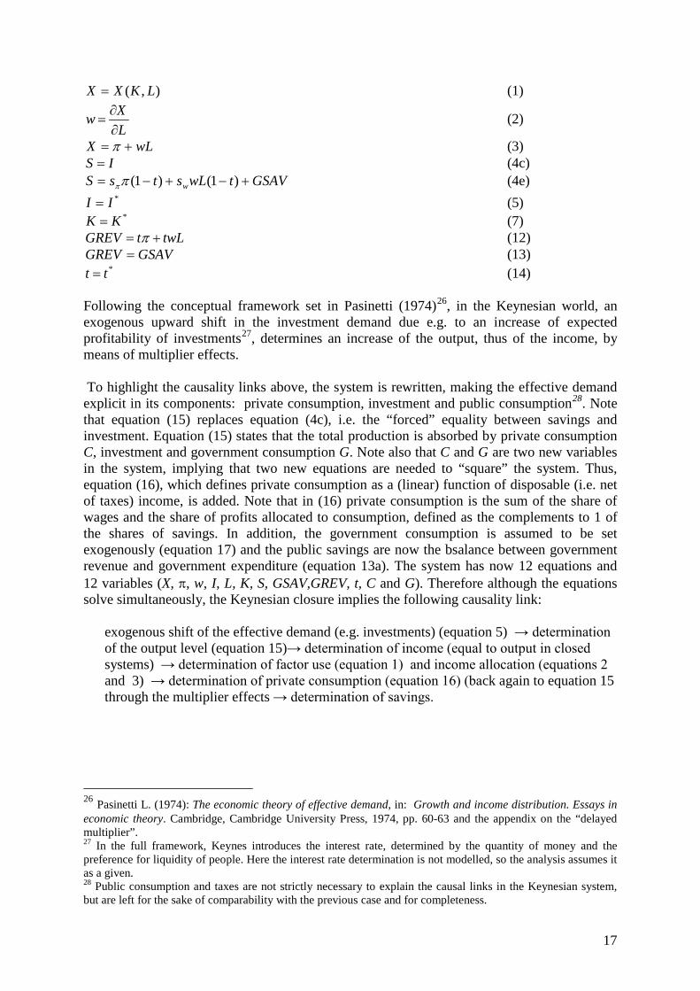
Following the conceptual framework set in Pasinetti (1974)26, in the Keynesian world, an exogenous upward shift in the investment demand due e.g. to an increase of expected profitability of investments27

, determines an increase of the output, thus of the income, by means of multiplier effects.

To highlight the causality links above, the system is rewritten, making the effective demand explicit in its components: private consumption, investment and public consumption28

. Note that equation (15) replaces equation (4c), i.e. the “forced” equality between savings and investment. Equation (15) states that the total production is absorbed by private consumption C, investment and government consumption G. Note also that C and G are two new variables in the system, implying that two new equations are needed to “square” the system. Thus, equation (16), which defines private consumption as a (linear) function of disposable (i.e. net of taxes) income, is added. Note that in (16) private consumption is the sum of the share of wages and the share of profits allocated to consumption, defined as the complements to 1 of the shares of savings. In addition, the government consumption is assumed to be set exogenously (equation 17) and the public savings are now the bsalance between government revenue and government expenditure (equation 13a). The system has now 12 equations and 12 variables (X, π, w, I, L, K, S, GSAV,GREV, t, C and G). Therefore although the equations solve simultaneously, the Keynesian closure implies the following causality link:

exogenous shift of the effective demand (e.g. investments) (equation 5) → determination of the output level (equation 15)→ determination of income (equal to output in closed systems) → determination of factor use (equation 1) and income allocation (equations 2 and 3) → determination of private consumption (equation 16) (back again to equation 15 through the multiplier effects → determination of savings.

26 Pasinetti L. (1974): The economic theory of effective demand, in: Growth and income distribution. Essays in economic theory. Cambridge, Cambridge University Press, 1974, pp. 60-63 and the appendix on the “delayed multiplier”. 27 In the full framework, Keynes introduces the interest rate, determined by the quantity of money and the preference for liquidity of people. Here the interest rate determination is not modelled, so the analysis assumes it as a given. 28 Public consumption and taxes are not strictly necessary to explain the causal links in the Keynesian system, but are left for the sake of comparability with the previous case and for completeness.

18

*II = (5) GICX ++= (15) ),( LKXX = (1)

LXw∂∂

= (2)

wLX +=π (3) )1)(1()1)(1( wstwLstC −−+−−= ππ (16)

GSAVtwLstsS w +−+−= )1()1(ππ (4e) *KK = (7)

twLtGREV += π (12) GSAVGGREV += (13a)

*tt = (14) *GG = (17)

In this framework, savings passively adapt to investment. This can be shown as follows: replace (3) and (16) into (15), to get:

GIstwLstwL w ++−−+−−=+ )1)(1()1)(1( πππ (15a)

Subtract to both sides of the equation (15a) equation (12) after substituting into that equation the (13a):

GSAVGGIstwLsttwLtwL w −−++−−+−−=−−+ )1)(1()1)(1( ππππ (15b) By transporting to the LHS all the elements of the RHS but investment, we get:

IGSAVstwLsttwLtwL w =+−−−−−−−−+ )1)(1()1)(1( ππππ With some manipulations on the LHS we get:

IGSAVstwLsttwLt w =+−−−−−−−+− )1)(1()1)(1()1()1( πππ

IGSAVstwLst w =++−−++−− )11)(1()11)(1( ππ Which reduces to:

IGSAVtwLsts w =+−+− )1()1(ππ (15c) Equation (15c) states the equality between total savings (private and public) as defined in equation (4e) and investment. Making use of equations (11) and (14) leads to:

**)1(*)1( IGSAVtwLsts w =+−+−ππ (15d) This implies that the equality between savings and investment is obtained by the solution of the abovementioned system for any level of investment, savings and fiscal decisions, by

19

means of the determination of appropriate levels of income, labour utilization and income distribution between profits and wages (equation 3). Table 1 summarizes the main features of the different models considered above. Table 1 Main features of alternative economic models Elements Neo-classical Keynesian Johansen Post- Keynesyan

(Kaldor-Pasinetti) Output Determined by

factor endowments and technology

Determined by the effective demand

Determined by the effective demand

Determined by the effective demand (or by factor endowments if full employment is reached)

Investment Endogenous Investment adapts to savings

Exogenous. Savings adjust to investments by means of changes in quantities and incomes (multiplier)

Exogenous. Savings adjust to investment by means of “compulsory” savings (taxes)

Exogenous. Income distribution adapts to adjust savings

Factors Full employment

May be unemployed

Full employment

May be unemployed

Wages Reflects MVP May not reflect MVP

Reflects MVP May not reflect MVP

4 Applying general equilibrium models for actual decision making In the light of the findings illustrated in the previous sections, when applying general equilibrium models to actual cases it is important to carefully analyze the macro-economic context and the factor endowments of the economic system. This relates for instance to the quantity and type of labour available, to the way labour markets work (or don’t work), in particular to their degree of geographic or qualitative segmentation, the level and causes of unemployment as well as to the way wages are determined in the specific institutional context. Analogous considerations hold for other factors such as capital or natural resource endowments such as land, water, mineral and other environmental assets. It is also important considering the degree of substitutability among various factors and the time span in which some substitutability could actually occur. Regarding the macro-economic context, it is important to understand the ways through which the macro-economic balances would be restored after the simulated shock and to what extent the country under investigation has the possibility to increase or decrease the balances of the macro-economic accounts, notably, the external debt and the government deficit. To understand the extent to which the different assumptions regarding the way an economic system works affect the model results, and, by way of consequence, policy making decisions, a simple general equilibrium model has been built. The model, whose main features are

20

illustrated in the next section, has then been applied to an “archetypical” (simplified) less industrialized economy.

4.1 A one-sector, two-household, two-factor general equilibrium model For illustrative purposes, the simple model refers to a one-sector, two-household, two-factor economy, open to international trade. The economy is “small” i.e. the country to which the model refers to is a price taker on international markets, which implies that the prices of imports and exports are set exogenously. The summary features of the model, including equations, endogenous and exogenous variables are represented in table 1. In the system, commodities flow from the producer to consumers, while services flow in the opposite direction. Flows of goods and services are countervailed by flows of payments. The commodity flow within the system is represented in figure 4. A domestic producer produces the one-commodity domestic output X , whose quantity is QX, sold at price PX , by means of one intermediate input, (the “composite” consumption good available in the system Q, whose quantity is QQ, bought at price PQ), and a factor aggregate (value added), combined by means of a “Leontief” technology, i.e. in fixed proportions with the output. The factor aggregate is obtained by combining labour services L, bought at price WL plus taxes on labour (social charges, etc) at a tax rate tl, and capital services K, bought at price WK, by means of a Constant-Elasticity of Substitution (CES) production function29

. The domestic producer operates under a “zero-profit” condition. The producer demands labour up to a point where the marginal value product of labour equates the labour wage. The same applies to capital. Equations G, H and I in table 2 set the behaviour of the producer and impose the zero-profit condition.

The one-commodity domestic output X is both sold on the domestic market and exported. However, imperfect transformation between the domestic and exported commodity is assumed. Quantities to be sold domestically and exported are set to figuratively maximize profits of a “transformer”, who buys the domestic output and transforms it in the export good E, where QE and PE are respectively the quantity and price of E, and in the domestic good DD, with QDD and PDD respectively the quantity and price of DD . This “transformation” occurs on the basis of relative domestic versus export prices and a Constant Elasticity of Transformation (CET) function, which establishes how one unit of domestic output can be transformed either in the domestic good or in the export good. The “transformer” operates under a “zero-profit” condition. PE is set as the international price of the exported good PWE times the exchange rate EXR, which is the price of one unit the foreign currency in domestic currency (units of domestic currency per one unit of foreign currency). Equations L, M, N and O set respectively the price of exports, the supply of exports, the supply of domestic good and the zero-profit condition of this figurative transformation process.

29 More complex production functions could be chosen which embody other types of capital services, such as human capital, natural resources such as land and water, or even immaterial assets, such as the quality of institutions. Implications of policies affecting the endowments and services of these resources, including policies to reinforce institutions would directly affect the domestic product. In this simple example, we consider only capital services and labour services to focus the attention on factor market and macro-closures, rather than on specific factors. In actual CGE models however, the extent to which factors actually affecting the production are included, influences the degree of adherence of the model to the reality and, by way of consequence, the usefulness of model results for actual policy making.

21

The domestic good DD however, is not directly consumed by the final consumers. The economic system also imports good the good M, where QM, and PM are respectively the quantity and price of M. PM is based on the international price of imports PWM, the exchange rate and a tariff rate on imports. Consumers demand the composite consumption good Q, where QQ, and PQ are respectively the quantity and price of Q. Q is a mix of imported and domestic goods, as the domestic and the imported goods are only imperfectly substitutable. The domestic good is therefore figuratively aggregated with the imported one by a “processor”. The mix is set to figuratively minimize the cost of the “processor”, on the basis of the price of the domestic good relative to the price of the imported good and a Constant Elasticity of Substitution (CES) function30

, establishing which quantities of import and domestic good are required for one unit of composite consumption good. Also the “processor” operates under a “zero-profit” condition. Equations P, Q, R and S in table 2, set respectively the price of imports, the demand of imports, the demand of the domestic good and the zero-profit condition of this figurative aggregation process.

30 This CES function in the literature is referred as the “Armington” function: Armington, P, (1969), A Theory of Demand for Products Distinguished by Place of Production. International Monetary Fund Staff Papers, XVI (1969), 159-178.

22

Figure 3. Production, transformation and processing of goods in the one-sector CGE.

Labour (L, PL)

Capital (K,PK)

CES

Value added Int.input (io*QX, PQ)

Domestic Output (QX, PX)

Leontief

CET

Final good (QQS,PQ)

Export good (QE, PE)

Domestic good (QDD, PDD)

Imported good (QM, PM)

Armington

Private consumers (QQD, PQ)

Investment (QINV, PQ)

Government (CG, PQ)

Interm. Cons (io*QX, PQ)

23

Table 2. A one-commodity, two-households open-small country general equilibrium model Eq.code #Eq Description of the equations Functional form #Var Endogen. var. Exogenous var. Notes

Households' consumption and supply of factorsA 2 Household demand of good QQh QQh*PQ*(1+tcon) = EXPh 5 QQh, EXPh, PQ Beta = 1, tcon One-good LES (share =1) B 4 Households' expenditure EXPh EXPh=Yh*(1-tins)-SAVh 7 SAVh tinsC 6 Income of households Yh Yh=Yh (WK,QKSh,WL,QLSh, UNEMPh, 16 WL,WK,UNEMPh QKS, QLS, REMFCh Labour income net of UNEMP

REMFCh, EXR TRGh, CPI, INTRAh) Yh, EXR, INTRAh TRGh,CPI

D 7 Labour price WL WL=WL (PLF, EXR) PLF, b (lab.mobility)E 8 Consumer Price Index CPI CPI=CPI(PQ,QQ) CPI = 1 is the numeraireF 10 Household savings SAVh SAVh = apsh*Yh*(1-tins) apsh, tins apsh: average prop.to save

F1 11 Equat.setting sum of intrah.transf.=0 INTRA1= - INTRA2

Producer of the basic goodG 12 Demand of capital of the domestic producer QK QK=#CES( QX, WK, WL) 18 QK, QX CES parameters CES-based factor demandH 13 Demand of labour of the domestic producer QL QL=#CES( QX, WK,WL) 19 QL CES parameters CES-based factor demandI 14 Zero profit condition of the domestic producer PX*QX = WK*QK + WL*QL + io*QX*PQ 20 PX io (technical coeff.) QX is the prod.of dom.output

GovernmentJ 15 Total government revenue GOVREV GOVREV=Y*tins+QQ*PQ*tcon+QM*PWM* 21 GOVREV tm, tl (tax rates)

EXR*tm + QL*WL*tl+FTRANSF*EXR PWM, FTRANSFK 16 Government expenditure GOVEXP GOVEXP = CG*CPI + TRF*CPI 23 GOVEXP, CG TRF The gov.exp.is exogenous

Import exportL 17 Price of exports PE PE = PWE * EXR 24 PE PWEM 18 Supply of exports QE QE = #CET(QX, QDD, PE, PDD) 27 QE, QDD, PDD CET parameters From the CETN 19 Supply of the transformed good QDD QDD = #CET(QX, QE, PE, PDD) CET parameters QDD goes from CET to CESO 20 Zero profit condition for the CET (the transformer) PX*QX = PDD*QDD + PE*QEP 21 Price of imports PM PM=(1+tm)*PWM*EXR 28 PM PWMQ 22 Demand of imports QM (Entering the CES) QM = #CES(QQ, QDD, PM, PDD) QM enters the CESR 23 Demand of the transformed good QDD QDD = #CES(QQS, QM, PM, PDD) 29 QQS QDD goes from CET to CESS 24 Zero Profit Condition for the CES (the "processor") QQS*PQ = PM*QM + QDD*PDD Armington CES aggregator

Market clearing and Macro closuresT 25 Labour market equilibrium QL = QLS - UNEMP U 26 Allocation of unemployment to households UNEMP1= LABSH1 * (UNEMP2/LABSH2) LABSHh LABSH1+LABSH2 = 1W 27 Capital market equilibrium QK= QKS X 28 Comodity market equilibrium QQ + QINV + ioQX + CG = QQS 30 QINVY 29 Trade balance QM*PWM=QE*PWE+FSAV+FTRANSF+REMFC 31 FSAVZ 30 Savings - Investment balance QINV*PQ = SAV + GSAV + FSAV*EXR GSAV

AA 31 Government buget balance GOVR - GOVEXP - GSAV = WALRAS 32 WALRAS WALRAS = 0 always In the table, variables referenced with the suffix h refer to each of the two household (h = 1, 2). The same variable without suffix refers to the sum across h. For simplicity, the table does not report neither the variables referring to the total across households as endogenous variables, nor the equations which set the totals across households, for instance, the table does not report neither the variable SAV (total household savings) among the endogenous variables nor the equation SAV=SAV1+SAV2 among the equations of the model.

24

Consumers demand the final composite good quantity QQ at the price PQ plus taxes on consumption at a tax rate tcon (equation A). A consumer price index CPI is created (equation E). Hoewever, being a one-good model, the CPI coincides with the price composite consumption good PQ . As the model is expressed in real terms, the CPI is chosen as the numeraire of the other prices and incomes and set equal to one. Each Household receive its income Yh (equations C) by selling labour and capital services, through remittances REMFCh from abroad, transfers from the government TRGh and intra-household transfers INTRAh. Expenditure EXPh on the final good for each household is set as income net of income taxes minus household savings SAVh (equartions B). Savings are calculated as net income times the average propensity to save, aps which is household specific (equation F). The labour supply QLSh is household-specific and exogenous. It includes also a foreign labour component LFh, exogenous as well, which gives rise to remittances. Remittances, based on the prevailing labour wage rate abroad, are received in foreign currency and converted in domestic currency by means of the exchange rate. The wage is endogenously set, the producer uses all the available labour, and the wage adjusts to a point where it equates the marginal value product of labour. The same applies for capital. This is imposed in the model by the equations of “optimal” demand of factors (CES-based). However, in its general form, the model is set in such a way that unemployment and exogenous wage setting (equation D) are allowed. If the wage is forced below its marginal value product, given the zero profit condition of the producer, the remuneration of capital increases above its marginal value. Vice-versa, if the wage is forced above its marginal value, the producer reduces its labour demand up to a point where the equality of the labour wage with its marginal value product is restored. This leaves part of the labour supply unallocated, giving rise to unemployment (labour clearing, equation T). In this case, the total unemployment UNEMP is allocated to households in fixed proportions, reflecting employment at the benchmark (Equations U). This implies that the labour income is given by the household supply of labour (exogenously set), net of its foreign component and unemployment (when it occurs), times the labour wage rate. In the model, the domestic labour wage is assumed to be determined on the basis of the prevailing wage in a closely related foreign labour market, assuming that there exists some institutional mechanisms allowing workers to push wages above the marginal value product of labour whenever the wage abroad, possibly adjusted to reflect the different working conditions and the degree of labour mobility, exceeds the domestic wage. The reverse applies for employers, when the foreign wage is lower than the domestic one. Taxes on income, consumption, imports and labour are collected by the government, which receives also transfers FTRANSF in foreign currency from abroad (foreign aid, exogenously set). The sum of taxes and foreign transfers gives the government revenue GOVREV (equation J). Government expenditure GOVEXP comprises the demand GC of the composite final good QQ, and monetary transfers from the government to households TRG, both set exogenously and fixed in real terms (equation K). The remaining equations are market clearing conditions and macro-closures. The first ones comprise: the clearing condition of the capital market, where the demand for capital services QK is equated to the sum of the supply from the two households LSK (equation W), and the clearing condition of the composite final good Q, (equation X) where its supply QQS is equated to the sum of the demand for final private consumption QQ, the demand for investment QINV, the demand for intermediate consumption ioQX and the demand for the

25

government consumption CG. The macro-closures comprise: the current account balance (equation Y), where the inflows of foreign currency due to exports plus the inflows from foreign transfers and the remittances minus the outflows for imports is gives: – foreign savings (- FSAV) (positive foreign savings implies a deficit of the current account balance, while negative foreign savings implies a surplus), the government budget balance (equation Z), where the government savings GSAV result from the difference between government revenue and government expenditure and the Savings-Investment balance (equation AA), where the investment expenditure is equated to the sum of savings of households, the government savings and the foreign savings multiplied by the exchange rate. This system comprises thirty-one equations and thirty-two endogenous variables, as reported in the sixth column of table 2. However, one equation is dependent from the others for the “Walras law”.31 A dummy “Walras” variable has been added to check for this dependency. Once calibrated on the Social Accounting Matrix (SAM) described in the next section, this system, will be adapted to test alternative macro and factor market closures and quantify relevant differences and related policy making implications32

4.2 An “archetypical” SAM of an aid-dependent less industrialized country.

.

The model described above has been calibrated on an aggregated Social Accounting Matrix (SAM) reflecting the one-year transactions of a foreign aid-dependent less-industrialized country33

. This SAM is assumed to be an archetype of the SAMs of poor oil-dependent countries with little or no mineral or timber resources, which base their inflows of foreign currency mainly on exports of agricultural products, foreign aid and to a minor extent on remittances. The weakness of the export sector, associated to the need to import essential goods, including medical appliances, drugs, technology items, in addition to oil and other energy products s well as fertilizers, lead to recurrent annual deficits of the current account balance. Furthermore, due to the high level of poverty and to institutional weaknesses, taxation is kept at very low levels while expenditures to ensure a minimum of social services generate government budget deficits. The SAM’s inflows and outflows and related structure, expressed as percentage of the totals of rows and columns respectively, are reported in table 3.

The main features of the “archetypical” aggregated and simplified SAM and the socio-economic system of reference are: 1. There is a single aggregated industry (activity) producing one aggregated commodity. 2. This commodity is both consumed domestically (96%) and exported (4%). 3. The same commodity is also used by the single industry as intermediate input, to produce

the unique domestic commodity (34% of the total output produced). 4. The final consumers (households, the government and investors -the S-I account-) require

the domestically produced commodity, but in addition require also that the commodity be imported. (87% and 13% respectively)

5. Factor income (labour wages and capital payments) are paid to households who provide services to the industry, as accounted by means of factor accounts.

31 A dummy “Walras” variable has been added to check for this dependency. 32 As the system is not “square”, to be solved in its general form reported in table 2, one endogenous variable needs to be exogenously determined (“fixed”). 33 The SAM reported in table 3 is essentially based on the Social Accounting Matrix of Burkina Faso for the year 2000, adjusted and simplified for some accounts, such as tax accounts, inventories and payments from factor accounts to financial and non financial enterprises.

26

6. Households are classified as poor (p) and non-poor (n), on the basis of their consumption expenditure compared with a poverty line34

7. Factor income (value added) is very unequally distributed between poor and non poor. 85% of the factor income is paid to non-poor people. As they are around the 50% of the population, on average they receive around five times more income than the poor people.

.

8. Labour Wages (which include family labour) distribute only 37% of the value added, while the payments for capital services distribute 63 % of it.

9. The government budget significantly depends on external support (high dependency ratio), as 44% of its revenue comes from the Rest of the World (RoW) as “foreign aid”. Despite these inflows, government savings are negative, showing a deficit of 22% of the total government inflows and affecting the S-I balance for -30% of the total savings.

10. Foreign aid constitutes 35% of the payments of the RoW to the country in the accounting period, the others being essentially loans (19%), signalling a deficit of the current account balance, payments for exports (33%) and remittances of migrants (13%)35

.

34 In the real-case matrix of Burkina Faso, the classification was done on the basis of the “Survey on the household living standards” in Burkina Faso in 2003, by adopting an absolute poverty line for the period April-July 2003 The poverty line, calculated on the basis of minimum calories intake and minimum-non food requirements, amounts to 82,672 FCFA per person per year, corresponding to around one fourth of the legal minimum wage and around two fifths of the international poverty line of one dollar per person per day. On the basis of this poverty line 46.4% of the population, corresponding to around 37.5% of the households was classified as “poor” (INSD, 2003: Profile de Burkina Faso la Pauvreté en 2003. au, Ministère de l’Economie et du développement. Segretariat General, Insitut National de la Statistique et de la Démographie (INSD). 35 Regarding the RoW account, the archetype SAM adopted here looks quite different form the “Social Accounting matrix for an archetype African Economy” chosen by Winters et al.(1996). There, no payments are recorded from the RoW to the S-I account (no foreign savings) and only 15.2 “Monetary Units-MU” over a total of 81.1MU of the RoW payments to the country (say, less than 19%) are paid to the government. Significant differences arise also in the share of value added distributed through wages, reported as 51%, compared with 37% in the SAM adopted here. Winters, P., De Janvry A., Sadoulet E., Stamoulis K, (1996). The Role Of Agriculture In Economic Development: Visible And Invisible Surplus Transfers Department of resource economics working paper n 143.

27

Table 3. Structure of an “archetypical” less-industrialized aid-dependent economy Panel A: Social accounting matrix

Activity Commodity Saving-Inv. Rest of the W.OUTPUT COUT LABOUR CAPITAL HOUS. Poor HOUS. Non-Poor GOVERNMENT S-I RoW Total

OUTPUT - 2,822,877 - - - 2,822,877 COUT 1,149,125 - 279,296 1,162,520 398,493 279,655 149,849 3,418,938

LABOUR 623,663 - - - - 623,663 CAPITAL 1,046,477 - - - - 1,046,477

HOU. Poor - - 129,301 129,173 - 38,581 11,795 - 18,440 327,289 HOU. NP - - 494,362 917,304 2,570 - 34,511 - 42,886 1,491,633

GOVERNMENT 3,611 137,904 5,297 56,048 160,368 363,228 S-I - 40,126 234,485 81,570 - 86,614 279,655

RoW 458,157 458,157 Total 2,822,877 3,418,938 623,663 1,046,477 327,289 1,491,633 363,228 279,655 458,157

Factors Insitutions

Panel B: Inflows’ Structure

Activity Commodity Saving-Inv. Rest of the W.OUTPUT COUT LABOUR CAPITAL HOUS. Poor HOUS. Non-Poor GOVERNMENT S-I RoW Total

OUTPUT - 100 - - - - - - - 100 COUT 34 - - - 8 34 12 8 4 100

LABOUR 100 - - - - - - - - 100 CAPITAL 100 - - - - - - - - 100

HOU. Poor - - 40 39 - 12 4 - 6 100 HOU. NP - - 33 61 0 - 2 - 3 100

GOVERNMENT 1 38 - - 1 15 - - 44 100 S-I - - - - 14 84 29 - - 31 100

RoW - 100 - - - - - - - 100

Factors Insitutions

Panel C: Outflows’ structure

Activity Commodity Saving-Inv. Rest of the W.OUTPUT COUT LABOUR CAPITAL HOUS. Poor HOUS. Non-Poor GOVERNMENT S-I RoW

OUTPUT - 83 - - - - - - - COUT 41 - - - 85 78 110 100 33

LABOUR 22 - - - - - - - - CAPITAL 37 - - - - - - - -

HOU. Poor - - 21 12 - 3 3 - 4 HOU. NP - - 79 88 1 - 10 - 9

GOVERNMENT 0 4 - - 2 4 - - 35 S-I - - - - 12 16 22 - - 19

RoW - 13 - - - - - - - Total 100 100 100 100 100 100 100 100 100

Factors Insitutions

4.3 Alternative macro-economic and factor market closures The abovementioned SAM has been used to calibrate the one-sector two-household two-factor CGE, notably, the efficiency and the share parameters of the CES and CET functions and the calculation of selected exogenous variables (remittances, transfers etc). Elasticities of substitution for the Armington CES and the CET for domestic-export transformation have been kept in the range 1 to 3, as discussed in Taylor (2006)36

No parameter was needed for the one-good LES consumer demand functions

, notably most simulations have been run with: 1) Armington elasticity of substitution between QDD and QM = 1.75; and 2) Elasticity of transformation between QDD and QE = -1.75. However, one scenario provides a sensitivity analysis of the results to changes of the Armington elasticity, which is set at 0.75. The elasticity of substitution between capital and labour at the bottom of the technology nest (figure 3) has been set at 1.5.

37

36 Taylor L, Arnim von R. (2006) Modeling the impact of trade liberalization. A critique of computable general equilibrium models. P.21. Oxfam research report July 2006.

.

37 With a one-good demand the issue of using price and expenditure elasticities compatible with Curnot and Engel aggregations reduces to imposing own-price elasticity and expenditure elasticity both equal to one. Also the issue of choosing the appropriate Frisch parameter compatible with own-price and income elasticities satisfying Curnot and Engel aggregation vanishes; indeed, the subsistence consumption waves out in the LES demand function when there is only one good. The Engel aggregation requires that the sum of the expenditure share times expenditure elasticity be = 1. If the share =1, the expenditure elasticity must be 1. This ensures that the share of the LES (the beta) is 1, as the beta in the LES demand is given by the expenditure share times

28

Considering the vulnerability of the economic system described above to external shocks affecting the balance of trade, it is interesting to analyze how the system adjusts to an upward shift of the aggregate import commodity price. . A 20% increase in PWM with respect to the base case has been simulated under the different macro-economic and factor markets closures. This simulation may reflect for instance the situation actually faced by most oil-importing less-industrialized countries, which, between 2003 and 2008 had to face a sharp and lasting increase of the international price of oil. The CGE described above has been implemented in GAMS. All the models are variants of the model reported in table 2. More specifically, the tested closures comprise the neo-classical model, five variants of “Keynesian” closures, a form of the “Johansen” closures and a form of “Kaldor-Pasinetti” closure38

. A synoptic view of the exogenous and endogenous variables and of equations dropped or included with respect to the general model of table 2 is provided in table 4. A detailed description of the different closures is provided here below. The results of the simulations are reported in table 5.

All the models exhibit a common result: the GDP does not change as a response to the import price shock. This is due to the fact that, one the one hand, for the neo-classical, Johansen and Kaldor-Pasinetti models, changes in GDP occur only if there is a change in factor endowments. On the other hand, in the Keynesian models changes in GDP occur if there are changes in the autonomous components of the effective demand, say consumption of the government CG and demand for investment I. For other aspects the models provide significantly diversified results. Neoclassical closure. In the neoclassical model, the equation setting the labour wage (equation D) and the equation allocating unemployment to the two households (equation U) are dropped. The two variables referring to unemployment (UNEMPp and UNEMPn) are dropped. In addition, by dropping both the equation setting intra-household transfers (equation F1) and fixing the intra-household transfers variables, the intra-household transfers are assumed to be exogenous. The exchange rate EXR is endogenous while the foreign savings FSAV are fixed to their benchmark value. The labour wage is free to move up to a point where it equates the marginal value product of labour. At that point, the production sector absorbs all the available quantity of labour QLS. The investment demand is endogenous. The shock on PWM affects the balance of trade (equation Y). Other things equal, QM reduces to restore the trade balance. This is due also to the fact that foreign savings FSAV are exogenous (fixed at the benchmark level). The appreciation of the exchange rate contributes

expenditure elasticity. The Curnot aggregation requires that the sum of the expenditure share of the good x times its own price elasticity plus the sum of shares of other goods times their cross price elasticities with x be equal to: minus the share of x. This implies that the expenditure share of x be =1. The other shares are 0, therefore: 1 * own price elasticity = -1. this implies that the own price elasticity = -1. Working out the Frisch paramerer compatible with such elasticities leads to conclude that any value for the Frisch parameter is compatible. Indeed, the subsistence consumption waves out in the LES demand function when there is only one good. 38 The reference to the various authors in naming the different closures does not necessarily imply a full adherence of the adopted model to the theories or visions of the authors themselves, as also discussed in Decaluwé et al. (1987), Decaluwé, B et al. (1987). Macro-closures in an open economy CGE models: A numerical reappraisal. Chaier 8704. C.R.D.E. Université de Montreal. For example, here the denomination “Kaldor-Pasinetti” is associated to a model of full employment not because these authors ruled out unemployment as a significant feature of real socio-economic systems but because we want to highlight the emphasis put on the income distribution changes, in presence of different propensities to save of different social groups, as an important adjustment factor of socio-economic systems hit by “shocks”.

29

to lower the domestic prices of imports, but at the same time depresses the price of exports39. Overall, an increase of PWM, through equation P reduces PM. Through the equation R (Armington) the demand of the transformed good QDD used to create the composite final good QQ increases. This implies that the exports QE decrease. The increase of the cost of the imports generates an increase of the price of the domestic final good PQ with respect to the domestic factors. Being PQ anchored to the numeraire CPI which is fixed to 1.00, this is reflected in an identical reduction of the prices of both capital and labour. The decrease in the price of factors generates a loss of income of both poor and non-poor. However, as the weight of the income from factors is smaller in the in the income of poor than in the income of non poor40

, the income of poor households reduces less than proportionally with respect to the income of non-poor households. This is reflected in the reduction of private savings, reduced consumption expenditure, reduced physical consumption and worsened Equivalent Variation (EV) both for poor and non-poor households. The above-mentioned differences in the structure of the income of poor households with respect to the non-poor ones, generates a greater percentage reduction in the equivalent variation of non-poor with respect to poor households. The government consumption CG is exogenous and fixed at the benchmark. This fact, associated to a reduction of the tax revenue, due to reduced income taxes and import tariffs, increases the government deficit GSAV. In turn, this fact, associated to the loss of private savings due to reduced incomes and the loss of foreign savings in domestic currency due to the appreciation of the exchange rate through the S-I balance (equation Z) reduces the expenditure for investment. This is a peculiarity of the neo-classical closure, where endogenous investments passively adapt to the available savings within the system.

Keynesian closures. The first four “Keynesian” closures differ from the neoclassical one in two fundamental aspects: 1) unemployment is allowed and determined on the basis of an “exogenously set” labour wage41

. Equations EQUNEMP and EQWAGE, (U and D in table 2) are included, allowing for the inclusion of two additional variables reflecting unemployment in the two households. 2) As in the “typical” Keynesian world, investment is set exogenously, i.e. no longer adapts to savings as in the neoclassical case. The differences among the first three Keynesian closures consist in a different treatment of government consumption, taxation and savings. The third “Keynesian” closure is probably the one which better reflect the “Keynesian” framework, where both investment and government consumption are exogenous and, domestic private savings are the only endogenous component of the Savings-Investment balance. The fourth closure is a replica of the third with a much lower Armington elasticity. The fifth “Keynesian” closure still allows for unemployment but fully endogenizes the labour wage.

Under “Keynes 1”, one component of the autonomous demand, notably the government consumption, is endogenous, together with the government savings and the foreign savings. As in the neoclassical case, an increase of PWM is reflected on PM. In addition now, the reduction in the foreign savings, implying a reduced supply of foreign currency, allows limiting the appreciation of the domestic currency, thus generating an even higher PM than in 39 A lower elasticity of substitution in the Armington CES would have implied a reduced appreciation or even a depreciation of the domestic currency with respect to the foreign one, as signaled for instance in ther simulation “Keynes 4”. 40 Conversely, the weight of the exogenous components (transfers from the government and from other households) is greater for poor than for non-poor households. 41 In the model, the wage is set on the basis of the wage level in foreign labour markets, as described in section 4.1. Note however that it is not fully endogenous, as it is assumed that workers look at the foreign wage converted in local currency through the prevailing exchange rate, which is endogenous.

30

the neoclassical case. Unemployment is now allowed. As the labour wage is not allowed to adjust with respect to the price of capital and the output as desired, unemployment emerges. The reduced employment and the reduced imports contribute to generate a reduction of the supply of final composite good QQ. On the other hand, as the capital factor is not allowed to be unemployed, its price reduces more than the price of labour. However, despite the change in relative prices, factor payments shift in favour of capital, as this remains fully employed42

. The reduction in the use of labour leads to a reduced domestic output. However, the reduction in the export price in local currency, due to the appreciation of the exchange rate, leads to a reduction of exports and to an increase of the transformed good absorbed by the domestic market. However this increase is not sufficient to compensate the reduction of the import due to the import price increase as the net combined effect of the appreciation of the exchange rate (reducing the import price) and the simulated shock (increasing it). Overall, this leads to a reduction in the supply of the composite final good which is stronger than under the neo-classical scenario.

In the current account balance, the simulated external shock on the import price (+20%), leads to an excess of foreign currency, due to: 1) the very price-elastic imports leading to a reduction of the outflow of foreign currency for imports with respect to the benchmark43 2) less than proportional reduction of export inflows with respect to the reduction of export outflows44

. Foreign savings FSAV need therefore to shrink to restore the current account balance equilibrium. However, the reduction of foreign savings leads to a “shortage” of savings in the S-I balance, reinforced by the appreciation of the exchange rate, because the investment demand QINV is exogenously fixed (anchored at its benchmark value). As also private savings shrink, due to shrinking factor incomes, government savings have to adjust to fill the gap in the S-I balance. This is done through reduction of the government deficit GSAV. The reduction of the government deficit, has to occur despite: 1) shrinking tax revenues due to reduced taxes on imports and reduced taxes on income; 2) reduced value of foreign transfers (foreign aid) in domestic currency, due to the exchange rate appreciation, which constitute a large component of the government budget. The deficit reduction is obtained by a reduction of government consumption CG more than proportional than the reduction of fiscal revenues. This leaves room to private consumption and investment demand. Overall however, under “Keynes 1”, due to some labour endowments left unemployed, the simulated import price shift hits the welfare (EV) of both poor and non poor households more than under the neoclassical closure.

When comparing the neoclassical closure with Keynes 1, it has to be noted that when foreign savings constitute a significant part of the total savings, as in the case of the archetypical economy under consideration, and they are fixed, as under the neoclassical closure, downward shifts in the exchange rate generated by shocks on international prices significantly reflect on the S-I balance, reducing the foreign savings in domestic currency. If this aspect is associated with endogenous investment demand, as in the neoclassical case, the investment demand is forced downward. If the investment is exogenous, as under Keynes 1, the domestic savings are forced upward. In this case, as private savings shrink due to shrinking income, 42 This can be easily seen by calculating the reduction in the factor payments, i.e. by multiplying the reduction of the wage times the reduction of the factor demand. For labour this amounts to: 0.975*0952=0.928, i.e. a reduction of 7.2%. For capital this amounts to: 0.943*1.00=0.943, i.e. a reduction of 5.7%. 43 The index of PWM times the index of QM amounts to 120.0*75/100-100=-10, i.e. -10.0%). As a result, the increase in the price of imports is more than countervailed by the reduction in the import quantities. 44 This results by multiplying the export price index times the export quantity index: (100.0*95.9/100-100=-4.1, i.e. -4.1%).

31

government savings have to increase to adjust the S-I balance. If tax rates are fixed, income is shrinking and import taxes shrink as well due to reduced imports, the increase of government savings has to occur through the reduction of the (endogenous) government consumption, as under Keynes 1. If foreign savings were only a marginal component of the S-I balance, as in less unbalanced economies, both the S-I balance and the government balance would be less sensitive to shifts of the exchange rate and shocks on the trade balance would have less impacts on the other macro-balances and in turn of the rest of the economic system. A similar consideration holds when looking at the impact of an exchange rate shift on the government budget in presence of a large amount of foreign transfers (e.g. foreign aid). Assuming exogenous and fixed foreign transfers, a downward shift of the exchange rate reduces the amount of transfers in domestic currency, reducing, other things equal, the government savings. But, for the considerations on the S-I balance above, savings have to adjust upwards. In practice, the adjustment of the government savings occurs upward or downward according to the relative importance of foreign savings with respect to foreign transfers, while the other endogenous variables affecting the S-I and the government balances bear the burden of the residual adjustments. Keynes 2 differs from Keynes 1 because here also the government consumption, in addition to the investment demand, is assumed to be exogenous. This is done through the endogenization of the aggregate income tax rate. However, government savings and foreign savings are still endogenous. The main difference here is that the proportional shift of the tax rates alters the expenditure distribution between poor and non poor, to the advantage of the poor, who at the benchmark pay a lower rate. Now, the government demand does not shrink as under “Keynes 1”, because it is exogenous (fixed at its benchmark level). This leads to an expansion of the labour demand because the reduction if imports due to their simulated price increase, is compensated by an increase of the demand of domestic transformed good, which in turn generates an expansion of the domestic output. Indeed, “negative unemployment”, which can be interpreted as a pressure on the labour market generated on the demand side, satisfied by some form of additional supply of labour45

, allows for a larger availability of the final composite good than under the Keynes 1 scenario. This is however absorbed by the government to the detriment of private consumption, generating worse EV indicators than under “Keynes 1”. Foreign savings, which are endogenous, shrink to accommodate the current account balance, as discussed under “Keynes 1”. Government savings increase to accommodate the S-I account. Direct adjustments of foreign and government savings do not allow adjustments of the savings through shifts in the income, which, by the way, is upward constrained by factor endowments, capital in this case.

Under “Keynes 3”, the supply of capital is endogenized, allowing the system to absorb all the quantity of labour and capital required to satisfy the effective demand. The government savings and the foreign savings are exogenized, so the domestic savings expand (or shrink) to a point where they match the investment demand, which is exogenous. In absence of

45 “negative unemployment” in this context has to be intended as additional labour requirements that would occur if the simulated price shock occurs and the model correctly interprets the economic system. As for simplicity we have assumed that at the benchmark there is no unemployment, this additional labour supply could come for instance from immigrants or from extra-hours worked, or the emersion of hidden unemployment (increased participation rate) etc.

32

constraints on the endowments, The S-I balance acts as the constraint to the expansion of the system46

.

A release of this constraint, through for example an exogenous increase of investment, on the one hand, requires and expansion of the domestic savings. On the other hand, the demand for investment activates the production process which requires more factors. Factor income expands, and both consumption and savings expand, with consumption demand giving rise to additional production. Overall, through the multiplier effect, production increases up to a point where the effective demand is satisfied and savings equate investment. The “Keynes 4” scenario replicates the “Keynes 3”, the only variant being a reduction of the Armington elasticity in absolute value from 1.75 to 0.75. This implies that a 1% decrease of the ratio PD/PM decreases the ratio QM/QD of 0.75 instead of 1.75, i.e. the system is less prone to substitute imports with domestic goods. Under this scenario the expansion of the final composite good is more limited than in the case of greater substitutability and factor demand shifts from labour towards capital. The fifth Keynesian closure drops the wage constraint and endogenizes GSAV while maintaining the aggregate income tax rate endogenous. Under this scenario, the final composite good drops dramatically, government savings significantly increase thanks to increases of tax rates, to compensate the decrease of private savings due to the fall of household income. “Johansen” closure. Under this closure, both capital and labour endowments are fully employed. Both government consumption and government savings and the aggregate income tax rate are endogenous, while investment demand, and foreign savings are exogenous. The endogeneity of the variables related to government plays a central role in bringing the system back to equilibrium after a shock. Comparing the “Johansen” with the neo-classical closure allows highlighting the role of the government in compensating the reduction of private savings and foreign savings. As investment is exogenous, also total savings are exogenously set as they have to comply with the S-I balance. Two facts emerge with respect to the neoclassical closure: 1) the gap in the S-I balance left by the downward shifts of the private savings and foreign savings in domestic currency, generated by the appreciation of EXR in presence of fixed FSAV in foreign currency, is compensated by an upward shift of government savings (indeed, a reduction of its deficit); 2) The purchasing power shifts from private households to the government (see the reduction in household expenditure w.r.t. the neoclassical case) thanks to an increase of the income tax rates of more than 40%. As non-poor exhibit at the benchmark a greater tax rate, this implies a reinforcement of the progressive tax scheme, to the advantage of the poor households (compare the consumption and EV indexes). This upward shift in government savings is generated by a simultaneous increase of tax revenues and a reduction of government expenditure. “Kaldor-Pasinetti”. This closure emphasises how income distribution changes, in presence of different propensities to save of different social groups, play an important role in the adjustment of the socio-economic systems hit by an external shock. Under this closure, the intra-household transfers (INTRAh) are endogenized. An equation setting the sum of intra-household transfers to zero is added to the model. Investment demand is exogenous and set to the benchmark. The external shock on import prices generates a loss of income, generating in 46 Under “Keynes 3”, analogously to Keynes 2, negative unemployment is generated, because unemployment is set at zero at the benchmark. This has to be read as an expansion of the labour demand. If unemployment was set at a positive value this would have amounted to a reduction of unemployment.

33

turn a loss of private savings. The S-I balance is restored through a transfer of income (indeed a reduction in transfers from non-poor to poor with respect to the benchmark) from poor households, who exhibit a lower propensity to save (12.6%) to non-poor households, who have a higher propensity (16.8%), thus restoring the S-I equilibrium. The shift of purchasing power is apparent when looking at the larger gap between the expenditure (and EV) of poor and non-poor households than the gap between their incomes. Under this closure both income taxes and intra-household transfers play this role. Here, negative taxes (subsidies) with higher rates for the non-poor play in favour of them, against the poor. A variant of this closure (not reported in table 5) implies leaving the burden only to shifts of the tax rates adjustment. Of course, the transfer of income has welfare implications as the welfare of poor households is negatively hit, while the one of non poor is boosted.

34

Table 4. Endogenous and exogenous variables relevant for setting alternative macro and factor market closures Var. Code Description # General Neoclass. Keynes 1 Keynes 2 Keynes 3 Keynes 4 Keynes 5 Johansen Kaldor-P.

Variables QKSh Supply of capital by household 2 X X X X ENDO ENDO X X XQLSh Supply of labour by household 2 X X X X X X X X XTRGh Transfers from govt to hous. 2 X X X X X X X X XGSAV Government savings (deficit) 1 X ENDO ENDO ENDO X X ENDO ENDO XFSAV Foreign savings 1 ENDO X ENDO ENDO X X X X XFTANSF Foreign Aid to government 1 X X X X X X X X XREMFCh Remittances by household 2 X X X X X X X X XCG Government consumption 1 ENDO ENDO ENDO X X X X ENDO ENDOUNEMPh Unemployment by household 2 ENDO X ENDO ENDO ENDO ENDO ENDO X XQINV Investment demand 1 ENDO ENDO X X X X X X XTY Aggregate income tax rates 1 X X X ENDO ENDO ENDO ENDO ENDO ENDOINTRAh Intra-households transfers 2 ENDO X X X X X X X ENDO

EquationsEQWAGE Wage equation 1 INCL DROP INCL INCL INCL INCL DROP DROP DROPEQUNEMPh Equation to allocate unemp.by hous. 1 INCL DROP INCL INCL INCL INCL INCL DROP DROPEQINTRAh Equat.setting sum of intrah.transf.=0 1 INCL DROP DROP DROP DROP DROP DROP DROP INCL * In its general form, the model presents one endogenous variable more than the number of independent equations. One variable needs to be exogenously determined (fixed”) to “square” the model and to make it solvable. In addition, for each equation dropped an additional variable needs to be “fixed”.

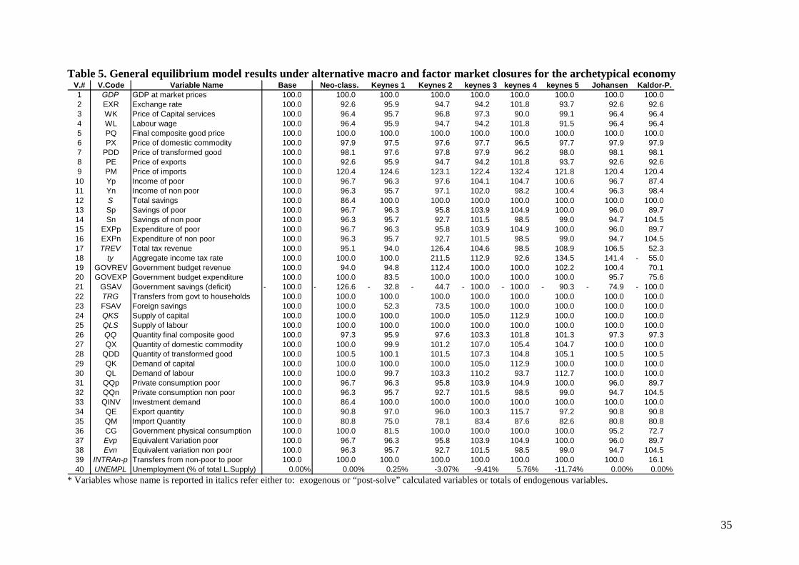
35

Table 5. General equilibrium model results under alternative macro and factor market closures for the archetypical economy V.# V.Code Variable Name Base Neo-class. Keynes 1 Keynes 2 keynes 3 keynes 4 keynes 5 Johansen Kaldor-P.1 GDP GDP at market prices 100.0 100.0 100.0 100.0 100.0 100.0 100.0 100.0 100.0 2 EXR Exchange rate 100.0 92.6 95.9 94.7 94.2 101.8 93.7 92.6 92.6 3 WK Price of Capital services 100.0 96.4 95.7 96.8 97.3 90.0 99.1 96.4 96.4 4 WL Labour wage 100.0 96.4 95.9 94.7 94.2 101.8 91.5 96.4 96.4 5 PQ Final composite good price 100.0 100.0 100.0 100.0 100.0 100.0 100.0 100.0 100.0 6 PX Price of domestic commodity 100.0 97.9 97.5 97.6 97.7 96.5 97.7 97.9 97.9 7 PDD Price of transformed good 100.0 98.1 97.6 97.8 97.9 96.2 98.0 98.1 98.1 8 PE Price of exports 100.0 92.6 95.9 94.7 94.2 101.8 93.7 92.6 92.6 9 PM Price of imports 100.0 120.4 124.6 123.1 122.4 132.4 121.8 120.4 120.4 10 Yp Income of poor 100.0 96.7 96.3 97.6 104.1 104.7 100.6 96.7 87.4 11 Yn Income of non poor 100.0 96.3 95.7 97.1 102.0 98.2 100.4 96.3 98.4 12 S Total savings 100.0 86.4 100.0 100.0 100.0 100.0 100.0 100.0 100.0 13 Sp Savings of poor 100.0 96.7 96.3 95.8 103.9 104.9 100.0 96.0 89.7 14 Sn Savings of non poor 100.0 96.3 95.7 92.7 101.5 98.5 99.0 94.7 104.5 15 EXPp Expenditure of poor 100.0 96.7 96.3 95.8 103.9 104.9 100.0 96.0 89.7 16 EXPn Expenditure of non poor 100.0 96.3 95.7 92.7 101.5 98.5 99.0 94.7 104.5 17 TREV Total tax revenue 100.0 95.1 94.0 126.4 104.6 98.5 108.9 106.5 52.3 18 ty Aggregate income tax rate 100.0 100.0 100.0 211.5 112.9 92.6 134.5 141.4 55.0 - 19 GOVREV Government budget revenue 100.0 94.0 94.8 112.4 100.0 100.0 102.2 100.4 70.1 20 GOVEXP Government budget expenditure 100.0 100.0 83.5 100.0 100.0 100.0 100.0 95.7 75.6 21 GSAV Government savings (deficit) 100.0 - 126.6 - 32.8 - 44.7 - 100.0 - 100.0 - 90.3 - 74.9 - 100.0 - 22 TRG Transfers from govt to households 100.0 100.0 100.0 100.0 100.0 100.0 100.0 100.0 100.0 23 FSAV Foreign savings 100.0 100.0 52.3 73.5 100.0 100.0 100.0 100.0 100.0 24 QKS Supply of capital 100.0 100.0 100.0 100.0 105.0 112.9 100.0 100.0 100.0 25 QLS Supply of labour 100.0 100.0 100.0 100.0 100.0 100.0 100.0 100.0 100.0 26 QQ Quantity final composite good 100.0 97.3 95.9 97.6 103.3 101.8 101.3 97.3 97.3 27 QX Quantity of domestic commodity 100.0 100.0 99.9 101.2 107.0 105.4 104.7 100.0 100.0 28 QDD Quantity of transformed good 100.0 100.5 100.1 101.5 107.3 104.8 105.1 100.5 100.5 29 QK Demand of capital 100.0 100.0 100.0 100.0 105.0 112.9 100.0 100.0 100.0 30 QL Demand of labour 100.0 100.0 99.7 103.3 110.2 93.7 112.7 100.0 100.0 31 QQp Private consumption poor 100.0 96.7 96.3 95.8 103.9 104.9 100.0 96.0 89.7 32 QQn Private consumption non poor 100.0 96.3 95.7 92.7 101.5 98.5 99.0 94.7 104.5 33 QINV Investment demand 100.0 86.4 100.0 100.0 100.0 100.0 100.0 100.0 100.0 34 QE Export quantity 100.0 90.8 97.0 96.0 100.3 115.7 97.2 90.8 90.8 35 QM Import Quantity 100.0 80.8 75.0 78.1 83.4 87.6 82.6 80.8 80.8 36 CG Government physical consumption 100.0 100.0 81.5 100.0 100.0 100.0 100.0 95.2 72.7 37 Evp Equivalent Variation poor 100.0 96.7 96.3 95.8 103.9 104.9 100.0 96.0 89.7 38 Evn Equivalent variation non poor 100.0 96.3 95.7 92.7 101.5 98.5 99.0 94.7 104.5 39 INTRAn-p Transfers from non-poor to poor 100.0 100.0 100.0 100.0 100.0 100.0 100.0 100.0 16.1 40 UNEMPL Unemployment (% of total L.Supply) 0.00% 0.00% 0.25% -3.07% -9.41% 5.76% -11.74% 0.00% 0.00%

* Variables whose name is reported in italics refer either to: exogenous or “post-solve” calculated variables or totals of endogenous variables.

36

5 Some policy implications Under the neo-classical closure with fixed foreign savings, in presence of significant amount of foreign savings, (i.e. deficit of the current account) as in the case of this archetypical economy, the appreciation of the exchange rate negatively affects the demand for investment through the variation of the value of foreign savings in domestic currency in the S-I balance. This contributes to leave more final output for private consumption, implying “better” household welfare indicators. While this result may lead to “optimism” in the short term, it hides longer term consequences for development perspectives. Less investment lead to less capital accumulation thus less production potential in the future. The Assumption that external shocks on international prices, associated to institutional rigidities on factors, may generate unemployment (the “Keynesian” closures), allows us providing a more realistic picture than assuming that factor markets will be able to absorb all shocks. However, the impact of an increase of import prices crucially depends on the way the economic system is able to substitute for imports with domestic products. Low capacities of substituting for imports are reflected in the model by a low elasticity of substitution (Armington elasticity). Low elasticities of substitution apply to all those commodities which cannot be produced domestically while are essential for the functioning on the economic system. In these cases, imported goods have limited or no substitutes, such as energy products in non-oil endowed countries or agricultural chemicals in non-producing countries. Low substitutability of imports in cases of external shocks on import prices badly reflects on welfare of households, investment possibilities and capacities of government interventions to redistribute income and provide good and services47

. In particular different assumptions on the elasticities of substitution between imported and domestic goods alter the impacts not only on the general level of welfare, but also its distribution. If we refer to an economy where factors are unemployed, (such as the one analyzed under the “Keynes 3” and “Keynes 4” scenarios in the previous section), different assumptions regarding the Armington elasticity imply also a different intensity in the use of factors. A lower elasticity of substitution, associated to wage rigidity in the labour market, is likely to leave more labour unemployed than in presence of a higher elasticity of substitution. This is also likely to shift factor payments toward capital.

The actual possibilities for a system to expand are linked to the existence of factors which can be mobilized. Hidden unemployment, in the form of underemployed family labour for instance, or even unconventional forms of capital, both man-made, natural and intellectual, such as biodiversity, specific climatic conditions, indigenous knowledge etc. may be put at work through appropriate policies. For the archetype economy described above, this in particular applies to sectors which can effectively provide import substitution. This is for instance the case of the energy sector which drains a large portion foreign currency of non-oil endowed countries, where actual substitution possibilities, such as bio-masses, solar technologies wind or water could help relaxing the current account constraint. However, models can provide responses on shifts in factor demands under a given policy scenario only to the extent to which these factors actually enter production functions. Unfortunately, some

47 This consideration is applies across all the closures tested. This conclusion is based also to simulation scenarios calculated by the author but not reported in table 5 for space reasons.

37

essential assets, such as environmental assets, or even appropriate institutions ensuring the correct functioning of markets, are difficult to quantify, thus often excluded by CGEs built for operational purposes. Therefore, constraints actually faced by real economic systems in absence of those assets are not reflected in models’ results. This implies that scenarios potentially doable according to model results, may prove to be undoable in practice, due to the missed inclusion of required production factors in the model. In all scenarios implying unemployment, an issue, not directly tackled by this CGE model is the income distribution between employed and unemployed. In situations where substantial increases of welfare of selected layers of the population are associated to significant increases of unemployment (such as the scenario described under “Keynes 4”), if poverty, an even, food security issues have to be avoided, redistribution mechanisms to ensure income support to unemployed need to be assured. Ensuring the direct public provision of services to the weaker layers of the population, in addition to ensuring equity, sustains the effective demand, generating multiplier effects which expand the output, and the income of the economy. On the other hand, situations where fiscal instruments, such as relatively high levels of income taxation (as in the Johansen 1 and 2 scenarios) drain to heavily on incomes of private agents resources that the welfare of people can be significantly negatively affected if fiscal resources are not used to sustain internal demand but used e.g. to fund too drastic international loan pay-back plans.

6 Conclusions In this paper, we analyzed the way different external shocks or policy measures affect an economic system, with the aim of identifying analytical implications relevant for policy making. Even economic policies, aimed at affecting specific segments of the economic system may have significant spill-overs and macro-economic impacts through the channels mutually linking production activities, factor markets, households, the government and the “rest of the world”. For this reason CGE models are widespread tools to simulate ex-ante the possible impacts of various policy options. However, the results of the simulations have to be interpreted in the light of the macro-economic and factor-related assumptions undertaken. An A detailed discussion of selected alternative macro-economic and factor market closure was carried out. However, the results of the alternative closure rules depend also on the structure of the economic system. For socio-economic development policy making it is important to better understand the extent to which the different closures affect the results of CGE models when they are applied to less industrialized countries. The SAM of a paradigmatic aid-dependent oil-importing less industrialized country has been chosen to calibrate a simple one sector-two-factor two household CGE model. Some tests with alternative closure rules have been carried out simulating the impacts of an international import price shock. Peculiar differences in the results emerged when contrasting “Keynesian” types of models, allowing for unemployment of factors with full employment models. Negative impacts of import price rises can turn out to be positive if it is assumed that factor endowments are not completely exploited and large or even relatively large elasticities of substitution between imports and domestic goods are chosen. In addition, given the importance of the foreign savings (the deficit of the current account) and foreign transfers (foreign aid) for this type of economy, the exchange rate plays a crucial role as it directly affects important components of both the Saving-Investment balance and the government balance. Alternative macro-and factor market closures have to be tested, as well as sensitivity analyses on elasticities whose actual level may be difficult to estimate, have to be carried out if proper use of general equilibrium models has to be made for actual decision making.

38

7 References Armington, P, (1969): A Theory of Demand for Products Distinguished by Place of

Production. International Monetary Fund Staff Papers, XVI (1969), 159-178.

Bellù L.G., Pansini R.V. (2009): Quantitative Socio-Economic Policy Impact Analysis: A Methodological Introduction. EASYPol series n.235.

Arrow, K and Debreu, G. (1954): Existence of a Competitive Equilibrium for a Competitive Economy. Econometrica 22 (3): 265-290

www.fao.org/easypol Food and Agriculture Organization of U.N -Rome.

Chenery, H.B. and Uzawa H. (1958): Non-linear Programming in Economic development. In Arrow,K. Hurwicz, L. an Uzawa H. (eds) Studies in linear and on-linear programming, Palo Alto CA. Stanford University press.

Deardorf A.V. and Stern R.M. (1986): The Michigan model of world production and trade: theory and applications. Cambridge. MIT press.

Debreu, G. (1959): Theory of value: an axiomatic analysis of economic equilibrium. New York, Wiley

Decaluwé, B. et al. (1987): Macro-closures in an open economy CGE models: A numerical reappraisal. Chaier 8704. C.R.D.E. Université de Montreal

De Melo, J. Robinson S. (1989): Product differentiation and the treatment of foreign trade in computable general equilibrium models of small economies Journal of International Economics, Volume 27, Issues 1-2, August 1989, Pages 47-67

Dixon, P.B, Parmenter, B.R., Sutton, J. and Vincent ,D.P. (1982): ORANI: a multisectoral model of Australian economy. North Holland, Amsterdam.

Harberger, A, (1962) The incidence of corporate income tax. Journal of political economy. 70: 215-240

INSD, (2003): Profile de Burkina Faso la Pauvreté en 2003. Ministère de l’Economie et du développement. Segretariat General, Insitut National de la Statistique et de la Démographie (INSD).

Johansen, Leif (1960): “A multi-sectoral Study of economic growth”. Amsterdam, North-Holland (2nd

Kaldor N. (1955): “Alternative theories of distribution”. The review of economic studies, pp 83-100.

enlarged edition, 1974).

Keynes J.M.(1936): The general theory of employment, interest and money. Electronic version, at http://homepage.newschool.edu/het//texts/keynes/gtcont.htm.

Merril, O.H. (1972): Applications and extension of an algorithm that computes fixed points of certain upper semi-continuous point to set mapping. Department of Industrial Engineering, University of Michigan.

Missaglia M. (2011): Neoclassical and Keynesian macro-models: Thinking about the special case. University of Pavia,(It). MIMEO

Pasinetti L.(1962): Rate of profits and income distribution in relation to the rate of economic growth. The review of economic studies, vol. XXXIX n.4, Oct 1962 pp.267-279.

Pasinetti L.(1974): The economic theory of effective demand, in: Growth and income distribution. Essays in economic theory. Cambridge, Cambridge University Press, 1974, pp. 60-63 and the appendix on the “delayed multiplier”.

Round J. (2003): Social Accounting Matrices and SAM-based multiplier analysis”, chapter 14 in F. Bourguignon and L.A Pereira da Silva (Eds): The impact of economic policies on poverty and income distribution, New York, World Bank and Oxford University Press.

39

Rattso, J (1982): “different Macroclosures of the Original Johansen Model and Their Impact on Policy Evaluation”. Journal of Policy Modelling 4(1) p.85-97.

Robinson S. (1989): Multisectoral models, (chapter 18) in Handbook of development economics, Elsevier.

Scarf, H.E. (1960): Some examples of global instability of the competitive equilibrium. International economic review, 1, 157-172.

Scarf, H.E. (1967): The approximation of fixed points of a continuous mapping. SIAM. Journal of applied mathematics. 15, 1328-43.

Sen A (1963): “Neo-classical and neo-Keynesian theories of distribution” Economic Record, March 1963, pp 53-64.

Showen, J.B. and Whalley J. (1972): A general equilibrium calculation of the effects of differential taxation on income from capital. Journal of public economics 1, 281-322.

Showen, J.B. and Whalley J. (1974): A proof of the existence o a general equilibrium with ad valorem commodity taxes. Journal of economic theory 8, 1-25.

Showen, B.J., Walley, J. (1992): Applying general equilibrium. Cambridge surveys of economic literature, Cambridge University Press.

Taylor L. And Lysy F.J (1979): Vanishing Income redistributions: Keynesian clues about model surprises in the short run. Journal of development economics, 6, (1979) 11-29, North Holland.

Taylor L. (1990): Structuralist CGE models, in Taylor L. (ed) ; Socially relevant Policy Analysis: Structural comptable general equilibrium models for developing world . Cambridge (MA): MIT press pp. 1-70.

Taylor L, Arnim von R. (2006): Modeling the impact of trade liberalization. A critique of computable general equilibrium models. P.21. Oxfam research report July 2006.

Thissen M. (1998): A classification of empirical CGE modelling, p.9. SOM Research Report 99C01, University of Groningen, The Netherlands.

United Nations, Statistical Division (1993): System of National Accounts. http://unstats.un.org/unsd/sna1993/toctop.asp

Van der Laan, and G., Talman, A. J (1979): A restart algorithm for computing fixed point without an extra-dimension. Mathematical programming 17, 74-84.

Walras, L. (1874): Éléments d’économie politique pure, ou théorie de la richesse sociale (Elements of pure economics, or theory of social wealth.) Lausanne, L. Borbax ed.

Willenbockel D. (1994): Applied general equilibrium modelling: Imperfect competition and European integration. Wiley.

Winters, P., De Janvry A., Sadoulet E., Stamoulis K, (1996): The Role Of Agriculture In Economic Development: Visible And Invisible Surplus Transfers Department of resource economics working paper n 143.