and analysis of a fluorescence spectrum for...
TRANSCRIPT

Molecular Imaging
and
Analysis of a fluorescence spectrum for determination of fluorophore depth
Master's Thesis by
Khaled Terike and Daniel Bengtsson
Lund Reports on Atomic Physics, LRAP-XXX Lund, January 2005

1
Abstract
In this study the goal was to map the field of molecular imaging and, especially, to find an
optical method, within molecular imaging, to recover the distance of a simulated fluorescing
lesion inside a tissue volume.
Spectral changes in the fluorescent light can be used to estimate the depth by measuring the
fluorescence signal in different wavelength bands. By performing a ratio between the signals
at two wavelengths we show that it is possible to determine the depth of the lesion.
Simulations were performed and validated by measurements on a phantom in the wavelength
range 815-930 nm. The depth of a fluorescing layer could be determined with 0.6 mm
accuracy down to at least a depth of 10 mm.

2
Contents
1. Backround and purpose.................................................................................... 4
2. Molecular imaging .............................................................................................. 5
2.1 Advantages of molecular imaging strategies ................................................ 6
2.2 Molecular imaging modalities and techniques .............................................. 10
2.3 Requirements for performing molecular imaging ......................................... 13
2.3.1 Probes ................................................................................................... 13
2.3.2 Overcoming deliver barriers ................................................................. 15
2.3.3 Amplification strategies ....................................................................... 15
3. Optical imaging .................................................................................................. 17
3.1 Fluorescence imaging .................................................................................... 19
3.1.1 Major factors affecting the flourophore performance .......................... 21
3.1.2 Advantages of the near infrared (NIR) spectral region ........................ 23
3.1.3 Probes for flourescence imaging .......................................................... 23
3.2 Bioluminescence imaging ........................................................................... 26
3.2.1 Probes for bioluminescence imaging ................................................. 26
3.3 Future outlook ............................................................................................. 28
4. Theory of light interaction in tissue .................................................................. 29
4.1 Light-tissue interaction .................................................................................. 30
4.1.1 Light ..................................................................................................... 30
4.1.2 Absorption ............................................................................................ 30
4.1.3 Scattering .............................................................................................. 31
4.1.4 Anisotropy factor .................................................................................. 31
4.2 Light propagation models – the forward problem ......................................... 32
4.2.1 The transport equation .......................................................................... 32
4.2.2 Solving the transport equation .............................................................. 33
4.2.3 The monte Carlo method ...................................................................... 33
4.3 The inverse problem .................................................................................... 34
4.3.1 Two-parameters methods ..................................................................... 34
4.3.2 The intergrating sphere method ............................................................ 36
5. Imaging deep interior tissue volumes ............................................................... 38
6. Analysis of a fluorescence spectrum for determination of depth................... 39

3
7. Material and method .......................................................................................... 41
7.1 MC-simulations ............................................................................................. 42
7.2 Tissue phantom ............................................................................................. 42
7.2.1 Preparing the liquis phantom................................................................ 43
7.2.2 Fluorescent layer .................................................................................. 43
7.3 Experiental phantom measurement ............................................................... 44
8. Results .................................................................................................................. 46
9. Discussion and conclusions ................................................................................. 49
Aknowledgments ..................................................................................................... 50
References ................................................................................................................ 51
Appendix 1 ............................................................................................................... 55
Appendix 2 ............................................................................................................... 57

4
1 Background and purpose
This thesis concerns the new, rapidly growing, biomedical field of research, Molecular
Imaging. Our tasks are: (1) to describe Molecular Imaging in general to give insight to this
new field of research in Lund. This study will mainly address the modality Optical Molecular
Imaging. A part within this field will be given extra attention, the evolution of so called
probes – molecules that are the core of the image signals. (2) The work also includes an
important contribution to the research‟s central part, imaging. Within this area we will attempt
to solve a problem within optical molecular imaging, to find a method which gives us depth
information from the signal which is obtained when a probe is activated. This is amongst
other things an important step towards eventually being able to reconstruct a tomographic
image through molecular imaging.
The first part of the essay gives an inroduction to Molecular Imaging. What has emerged from
the field along with potential fields of applications is described here. This section also treats
the requirements for performing Molecular Imaging. The imaging modalities PET (Positron
emission topography), SPECT (Single photon emission computed topography), MRI
(Magnetic resonance imaging), CT (Computer topography) and ultrasound are not treated in
any greater extent in this essay.
The next big section, Chapter 3, specifically treats optical molecular imaging. A more in-
depth description of light emitting probes and how the signal is brought forth is given here. A
couple of successful experiments within MI are also described in this chapter.
Chapter 4 concerns the interaction between light and tissue from a theoretical point of view as
well as definitions of useful parameters within tissue optics. Finally, a description of the
disposition and thought behind the experimental tests are given (Chapter 5 & 6) and later
presented and discussed in Chapter 7 and 8.
The results of the completed experiments have been published in the article “Fluorescence
spectra provide information on the depth of fluorescent lesions in tissue” which is found as an
attachment to this essay.

5
2 Molecular Imaging
To explore things we cannot see with our own eyes has for long been of great interest to man.
Through the history new imaging techniques have played an important role in the
understanding of how our world is constructed and how it works. Imaging with x-rays has
been revolutionary for making diagnosis within medicine. The telescope is another imaging
tool, which really has broadened our horizon and given us pictures from parts of our world
that were unexplored for long.
For biologists the study of the form and structure of organisms and its parts relies on
observations with microscopes. Molecular imaging is a biomedical research discipline that
extends such observations in the living body of a plant or animal to a more meaningful
degree. The images reflect in vivo biologic processes at the cellular and molecular levels in
their native environment.
Molecular imaging is a complex field that requires knowledge from many different research
fields; Biology, chemistry, medicine, pharmacology, medical physics, mathematics and
informatics are all necessary parts of this new imaging model. Recent developments of
different image-capture techniques belong to the central core of molecular imaging. See figure
2.1 below.
Figure 2.1. Molecular imaging is a multidisciplinary field that requires broad knowledge to conduct.
Present imaging technologies rely mostly on physiological or metabolic changes for
distinguishing altered from normal tissue. With molecular imaging the focus is moved one
step further; the molecular abnormalities that are the basis of the disease are investigated,
rather than the end effects of such molecular alterations. This change from a non-specific to a
specific approach describes an important progress where imaging can be used for better
understanding of biology, for earlier detection of disease, and for evaluating treatment
outcome.
Molecular imaging has emerged from recent advances in molecular and cell biology
techniques, development of new imaging instrumentation such as positron emission
topography (PET), magnetic resonance imaging (MRI) and optical imaging and the possibility
of purposely transfer genes between organisms (especially to mice). Also, the availability of
new contrast enhancing agents, that are highly specific, is a fundamental part within the field.

6
The goals possible to achieve in biomedical research, thanks to the development of molecular
imaging are: (a) being able to study specific cellular and molecular processes taking place in
the living body of an animal (in vivo), without involving entry (noninvasively); (b) to watch
multiple molecular events that occurs within a short time; (c) to follow targeting or trafficking
of cells; (d) to optimise drug therapy; (e) to image the effects different drugs have on
molecular and cellular level; and (f) to evaluate and map disease progression at molecular
level. Specifically, molecular imaging is considered to be an extraordinary opportunity for
research in cancer1.
Molecular imaging has its roots within nuclear medicine. Nuclear medicine is a discipline
focused on labelling substances in the human body with radiotracers and in such manner
follow and map those roles. In today's molecular imaging, the principle is the same but has
been extended to other imaging modalities as well and consequently other sources for contrast
than radiotracers. The imaging modalities that have been used until now are CT (computer
topography), MR imaging (magnetic resonance imaging), nuclear imaging techniqes (PET,
SPECT and gamma scintigraphy), nanosensors, optical imaging and ultra sound. The different
imaging modalities are suitable for diverse purposes and the probes that are developed are
designed according to which modality is to be used. In Ref 32 a number of gene products with
corresponding suitable imaging technique are described.
The physicist role in molecular imaging is mainly the development and management of the
advanced imaging technology used, but also in the interpretation of the captured signals and
the reconstruction of clear and understandable images.
2.1 Advantages of molecular imaging strategies
In order for a physicist to understand the advantages molecular imaging provide it is
important to be familiar with how biomedical research is pursued today and what limitations
it faces. Along with some terminology this section will give some briefing on the subject.
The nucleus of the cell contains the genetic information of a human being. This information is
kept in the chromosomes that are built up by DNA stands. Some of this information is used to
express proteins. The proteins have many important functions in the body; structural and
regulative among others. For a protein to be expressed the information in the DNA (genes)
has to be encoded. The DNA is for this purpose transcribed into RNA - a new molecule that is
a copy of the DNA. The RNA acts like a template for the proteins that are put together at the
ribosomes.
If any of those steps goes wrong, undesired proteins will be formed, affecting the important
functions they have. In cases when the body is unable to remove such mistakes they can give
rise to disease3.
Revolutionary with molecular imaging is that these proteins can be tracked and imaged. This
is done by means of probes with a signal-emitting particle (e.g a fluorchrome or radioactive
particle). By finding a protein that is expressed at a certain disease, it will be easier to develop
drugs that stop those proteins from being effective. If cancer is caused by the defect gene the
proteins can be imaged to follow its metastasis etc. Using protein tagging for mapping the
distribution of an animals own proteins servers as another example of the potential this

7
method has. Mapping the distribution of proteins and enzymes can be used to track embryotic
development in action – to see at exactly what point different enzymes get turned on in cells4.
There are, however, further advantages of using highly specific probes. Imaging of proteins,
enzymes and other biomolecules can be used to study the genes from which they emanate.
This kind of research is referred to as gene expression studies. The answers scientists seek by
studying gene expression are very profound; What function does a certain gene have? Did we
manage to replace a defect gene successfully? Or; does a patient have genetic material that
could be dangerous? Gene expression (figure 2.2) is best understood by describing how defect
genes can be replaced (gene theraphy) and by decribing how a specific genes function is
found out in present research3.
To cure a defect gene, the damaged part of the DNA must be replaced with an intact replica.
To produce this replica mRNA (messenger RNA) from a healthy cell is taken. In a laboratory
this mRNA is transformed into complementary DNA (cDNA). This is done via an enzyme
called reverse transcriptase. In the next step this cDNA is copied to DNA templates. The last
step is to introduce the DNA into the defect cell and wait for the cell to begin expressing the
new, undamaged, genetic information. Integrating the DNA into a delivery vehicle makes
introduction of the DNA possible. The delivery vehicle, or vector, could for example be a
virus3.
Figure 2.2. Gene expression. Process where the coded information in a gene is converted into many of the
structures present and operating in the cell. Expressed genes are first transcribed into mRNA and then into
proteins. Modified from Ref 3.

8
It is, however, not trivial to tell whether a gene has been replaced successfully or not. One
could imagine the construction of a probe that tags and is activated by interaction of a protein
coming out from the undamaged gene, but that is insensitive to proteins expressed from the
damaged gene. In such manner a successful gene transfer could be tested. However, some
proteins are more difficult to track than others, and this method implies a great deal of work
since developing a new probe for each target (replaced gene) would be necessary. A
complementary method is therefore often used. Along with the healthy, undamaged, DNA
that is introduced in the cell, additional genetic material is included. The additional material is
a so-called reporter or marker gene - a gene that encodes for an easily detectable protein. So,
if the DNA is replaced successfully, a well-known detectable protein will also be expressed
(figure 2.3). It is important for gene therapists to know what cells the gene is going into and
where it is being expressed4.
This method can not only be used for validating if a gene is successfully transferred. Also, it
can be used generally to determine the patterns of gene expression that encode normal
biological processes, or, by transferring genes that have unknown functions, to find out
certain genes functions3.
Figure 2.3. Along with the genetic material that is going to be expressed a reporter gene is delivered (1). If the
delivery is successful an easily detectable protein is expressed that can be marked i.e. by a intravenously injected
probe (2). The gene delivery can then be imaged (3).
Within molecular imaging there are two classes of marker genes that have been used for
investigation: (a) marker genes encoding intracellular enzymes and (b) marker genes encoding
cell-surface proteins or receptors. Intracellular expressed proteins has the advantage of being
relatively invisible for the immune system whereas surface-expressed receptors are easier to
detect since the probe not necessarily need to penetrate into the cell. Neuroscientists have
used radio-labelled probes that bind to some types of receptors that are placed on the surface
of nerve cells in the brain. In such manner they have managed to map nerve cells that use
dopamine and serotonin4.
Researchers are also looking for another technique that would have far broader applications:
imaging the expression of native genes. The idea is to use probes that bind to mRNA-
molecules. mRNA are the molecules that turn on the production of proteins in cells. This
would help doctors to tell whether patients are expressing particular genes. By looking at
reduced effect of the genes that enable cancer cells to multiply rapidly, doctors could measure
the effectiveness of cancer therapy4.

9
Some biotech companies have developed molecules that bind to mRNAs from such genes in
order to block the production of the proteins they code5.
The development of high-affinity probes and marker genes is a fundamental part of molecular
imaging. It implies great progress within all types of biological research but what differs
molecular imaging from conventional techniques is its applicability to living subjects.
Defining gene expression pathways is at present successfully done using conventional in vitro
and cell culture techniques. Despite the success and rapid progress these conventional
techniques have implied molecular imaging provide further advantages for these kinds of
studies.
In many cases the outcome of a certain gene is not only dependent on the genotype, but also
influenced by environmental factors. The predicted outcome of a gene, from in vitro studies,
can be quite different when studied in a living animal1. In vivo molecular imaging provides
the opportunity to study what effect those additional factors, such as physiological whole-
body contributions of proteins, have in the biological pathways. The function and interaction
of a specific gene becomes more realistic when studied in intact animals where the biological
system is complete, and the complex biological network is not overlooked.
Molecular imaging in intact living animals can, as mentioned, also be of benefit within
pharmaceutical research. In combination with transgenic animal models, the discovery of new
drugs becomes easier. Because this kind of studies includes effects of transport/delivery,
metabolism and excretion, new drugs can be excluded or accepted quicker than before.
Molecular imaging facilitates validation of the target protein, evaluation of test compounds,
studies of toxiological effects of the drug and testing its efficiency1.
The possibility to perform repetitive studies of the same animal is a further advantage over in
vitro and cell culture experimentation. The studies can be performed at different time points,
with the same or with different molecular imaging modalities, all in the same animal. This
gives a clearer vision of how biological parameters under examination change over time. This
yields better results from fewer experimental animals.
Molecular imaging and standard use of conventional imaging can complement each other in a
satisfying way. A good example of this is described by Bremer et al. (Ref 6). Here two
equally sized tumours have been implanted in a mouse one which is more aggressive than the
other one. With MRI the exact position and size of the tumours can be revealed but it does not
provide any information about the aggressiveness. A probe designed to tag a protein which is
only expressed in the more aggressive tumour is designed. The probe is fluorescent and
reveals the difference between the tumours. If only molecular imaging would have been used
just one of the two tumours would have been visible.
The ability to perform both tomographic imaging and quantitative measurements over time
(four-dimentional information) could be possible with molecular imaging without being too
time consuming. However, more research is required within this field.

10
2.2 Molecular imaging modalities and techniques
The development of new clinical imaging technologies has made rapid progress the last
decade. The research has concentrated on changing focus from in vitro to in vivo imaging. Of
special interest has been development of technology that allows non-invasive, high-resolution,
small-animal imaging. Small systems are very useful when conducting laboratory studies
within molecular imaging since they are relatively simple and inexpensive in contrast to the
corresponding used for clinical purposes. However, an important issue and challenge within
research on imaging technology is how to further expand this instrumentation and techniques
so that it becomes applicable to human studies.
In small animal research one aims to obtain as high signal as possible with a high temporal
resolution and with minimum amount of probe. The goal is ultimately to develop a single
device that produces three-dimensional images of anatomical and biological information
together. So far there is no such device but one must choose the most suitable for the
experiments meant to be conducted. The characteristics that separate different instrumentation
form each other are:
resolution (spatial and temporal)
depth penetration
energy expended for image generation
This depends on which component of the electromagnetic spectrum is utilized for
generating images, i.e. ionizing such as CT (-rays) and PET (-rays) or non-ionizing
such as optical imaging (visible or NIR light) and MR (radio waves).
whether there are injectable/biocompatible molecular probes available, and
sensitivity of the system
The sensitivity basically tells which the least detectable amount of probe is.
In table 1 below all available imaging modalities are mentioned with corresponding
characteristics. Further discussion will not be conducted in this text but for more reading on
the subject the internet page http://www.mi-central.org is recommended.

11
Table 2.1. Characteristics of imaging modalities available1
Imaging technique
Portion of EM radiation spectrum used in image generation
Spatial resolution
Depth Temporal resolution
Sensitivity Type of molecular probe
Amount of molecular probe used
Positron emission topography (PET)
high-energy
rays
1-2 mm no limit 10 sec to minutes
10-11-10-12
mole/L
radiolabeled, direct or indirect
nanograms
Single photon emission computed topography (SPECT)
lower-energy
rays
1-2 mm no limit minutes 10-10-10-11
mole/L
radiolabeled, direct or indirect
nanograms
Optical biolumine-scence imaging
visible light
3-5 mm 1-2 cm seconds to minutes
possibly
10-15-10-17
mole/L
activable indirect
micrograms to milligrams
Optical fluore-scence imaging
visible light or near-infrared
2-3mm 1cm seconds to minutes
likely 10-9-
10-12 mole/L
activable direct or indirect
micrograms to milligrams
Magnetic resonance imaging (MRI)
radiowaves
25-100 m no limit minutes to hours
10-3-10-5 mole/L
activable direct or indirect
micrograms to milligrams
Computer topography (CT)
X-rays
50-200 m no limit minutes not well charachterized
may be possible
not applicable
Ultrasound high-frequncy sound
50 - 500 m millimeters to centimeters
seconds to minutes
not well charachterized
limited activable, direct
micrograms to milligrams

12
Imaging technique
Quantit-ative degree
Ability to scale to human imaging
Principal use
Advantages Dis-advantages
Cost
Positron emission topography (PET)
+++ yes metabolic, reporter/gene expression, receptor/ligand, enzyme targeting
high sensitivity, isotopes can substitute naturally occurring atoms, quantitative translational research
PET cyclotron or generator needed, relatively low spatial resolution, radiation to subject
****
Single photon emission computed topography (SPECT)
++ yes reporter/gene expression, receptor/ligand
Many molecular probes avaliable, can image multiple probes simultane-ously, may be adapted to clinical imaging systems
relatively low spatial resolution because of sensitivity, collimation, radiation
***
Optical biolumine-scence imaging
+ to ++ yes but limited
reporter/gene expression, cell trafficking
highest sesitivity, quick, easy, low-cost, relative high-throughput
low spatial resolution, current 2D imaging only, relatively surface-weighted, limited translational research
**
Optical fluore-scence imaging
+ to ++ yes but limited
reporter/gene expression, cell trafficking
high sesitivity, detects fluorochrome in live and dead cells
relatively low spatial resolution, surface-weighted
*-**
Magnetic resonance imaging (MRI)
++ yes morphological reporter/gene expression, receptor/ligand if many receptors
highest spatial resolution, combines morphological and functional imaging
relatively low sensitivity, long scan and postprocessing time, mass quanty of probe may be needed
****
Computer topography (CT)
not applicable yes morphological bone and tumor imaging, anatomical imaging
limited "molecular" applications, limited soft tissue resolution, radiation
**
Ultrasound + yes morphological real-time, low cost
limited spatial resolution, mostly morphological
**

13
2.3 Requirements for performing molecular imaging
Analyzing tissue samples ex vivo is relatively easy compared to corresponding studies
conducted in living subjects. Ex vivo studies are done using test tubes that contain cell
extracts or intact, cultured, living cells. Different cellular processes can be tested by means of
reagents added closely to the cells or even injected into the proper cell. To image specific
molecules in vivo is more of a challenge. Several criteria must be met after an appropriate
target has been selected:
A molecular imaging probe must be developed. The task of the probe is to distinguish the
particular biological process and help to generate images of the target. The probes must
have the right chemical, biochemical and molecular properties to manage this in vivo.
The probe must posses the ability to overcome biologic delivery barriers. Such barriers
could be the cell membrane, of interstitiala or vascular
b nature.
An amplification strategy must be used so that the concentration of the probe is
sufficiently large after interaction of the target.
Sensitive, fast, high-resolution imaging techniques must be available.
2.3.1 Probes
Molecular probes provide the signal in almost all molecular-imaging assays. The only
exception is MRS, which is a spectroscopic method for analysing tissue. MRS belongs to the
same family as Magnetic resonance imaging (MRI). The signals constitute the spectra which
emanate directly from the molecules in the tissue under examination.
Probes used for molecular imaging are injected into the living subjects to image specific
molecular and biological events. A probe typically consists of two components coupled
together; one that interacts with the target and one that emits a signal. The interacting
component should have as high affinity as possible to the target so that the probe accumulates
in large amounts where the target is present and exclusively in these regions. This component
is often referred to as delivery vehicle. The signalling component is for tracking the probe so
that the target can be imaged. The nature of the signalling component depends on which
device is used for capturing the signal. In radio labelled approaches it is often a single atom
with radioactive properties (such as FC 1811 , or Tcm99 ) that is attached to the delivery vehicle
whereas in optical approaches fluorescent molecules (fluorochromes) are used. For MRI the
signalling component is some kind of paramagnetic atom1.
Probes can be categorized as radio labelled or activable probes. Radioactive probes (for PET
and SPECT imaging) produce a signal continuously, before and after interacting with their
target. Activable probes emit a signal only after interaction with the target and are
undetectable before. These probes are used for optical imaging among others. This is a broad
categorization that covers most available probes and some further classification could be
a Interstitial - Characteristic of a particular organ or tissue. b Vascular - Relating to a channel for a body fluid; especially blood vessels.

14
useful. Due to difficulties for the probes to reach their targets (see section 2.3.2) some probes
are less direct than others. Instead of interacting directly with the target, indirect probes are
made to image substances associated with expression of the target.
Molecular imaging probes can be small molecules such as receptor ligandsc or enzyme
substratesd, or higher-weight affinity ligands (figure 2.4). Examples of the latter are
monoclonal antibodies and recombinant proteins. Monoclonal antibodies are proteins with a
definite structure that binds antigense and are made by cell culture technique. Recombinant
proteins are genetically engineered proteins7.
.
Figure 2.4 (Modified from Ref 7). Biological molecules for targeting/imaging. Higher-weight affinity ligands
such as antibodies (proteins), peptides (molecule composed of up to 20 amino acid residues joined by peptide
bounds) and aptamers (nucleic acids) are suitable delivery vehicles for molecular imaging probes. Small
molecules (~300u) are characterized by high specificity, high affinity binding to receptors, transporters or
enzymes and rapid distribution/clearance (minutes/hours). Heavier molecules (antibodies ~150 000u) have high
affinity to a variety of targets and slow distribution/clearance (days/weeks).
The most common type of probes are the non-specific with vascular distribution, e.g.,
circulating within blood vessels. Most of the contrast media in conventional medical imaging
is of this kind, but they are also being used in radionuclide and optical imaging. Indocyanine
green is a widely used fluorescent contrast agent that belongs to this group. They can be used
to image physiological processes such as flow and changes in blood volume but cannot image
specific biological processes at cellular or sub-cellular level. Still they are useful for studying
"downstream" changes in disease process although not suited for monitoring the very early
alterations8.
For better targeting potential, probes can be made using substrates that can interact with
targets within cells or with separate sub-cellular sections. For this purpose antibodies or

15
cligands are used. These kinds of probes are the second most common and are mainly used for
radionucleic and optical imaging. The probes can be used to image the end products of gene
expression by letting the probe interact with the original protein expressed from a specific
gene. The limitation of this approach is the rather difficult and expensive development of
these probes. For each new protein to be targeted a new substrate must be discovered and
radio-labelled. It is desirable to discover a method that could image gene products from any
gene of interest and many research groups have put effort in putting reporter gene/reporter
probe systems together in order to decrease the amount of work for this kind of research1.
The probes mentioned above have one major drawback: background noise can disturb the
measurements with such probes. The first mentioned type of probes, the non-specific with
vascular distribution, give rise to a signal independently of where in the living body the probe
is, even in their activable mode (i.e indocyanine green). Neither, for the second kind of
probes, can a bound probe be distinguished from one which has interacted with its target. In
order to bypass this, other probes have been developed. Probes with these characteristics are
especially so-called smart probes and optical reporters. These probes are especially suitable
for optical imaging and will be discussed under sections 3.1.3 and 3.2.1.
2.3.2 Overcoming deliver barriers
Molecular imaging probes face many obstacles well inside the body. In order to reach the
target in sufficient concentration and to stay there long enough it has to avoid being
transported away, fragmentation and overcome delivery barriers. Overcoming delivery
barriers is the most challenging and several strategies have been developed to make this
possible. The probe could be made more "invisible" for the body by decreasing its sensitivity
to immune response, which gives it more time to reach the target without being carried away
or recognised immediately. At the cell surface mechanisms that shuttles the probe into the cell
can be utilised. Smart probes are often made long circulating in order to achieve a more
homogeneous distribution. Long circulating times are usually not desirable, but smart probes
are built up from a main structure (copolymer chain) that helps the probe to reach cells by
slowly passing from the blood vessels into the surrounding tissue9. Local delivery is another
way of bypassing delivery barriers.
2.3.3 Amplification strategies In molecular imaging the amount of targets can be very limited, and it is important that the signal from the probe is as strong as possible. A signal emanating from deep inside a body faces many obstacles, preventing it from reaching the detector. To deal with this problem different amplification strategies can be used. When possible, as many signal emitting particles per probe is one way to facilitate detection. This strategy is used for smart probes that are described in section 3.1.3 along with a successful example of molecular imaging. To choose targets carefully is another way of minimizing this problem. For instance, if the intention is to visualize a cancer tumor it is appropriate to choose a target that is not only associated with the tumour but also expressed in c Ligand - For a single larger molecule or receptor site, any of the smaller molecules or ions that are able to bind with the larger molecule or site. d Enzyme - Biologic macromolecule that acts as a catalyst by lowering the activation energy of a reaction. Enzymes are proteins or RNAs. A substance that an enzyme acts upon is an enzyme substrate. e Antigen - Any material that is dissimilar to structures in an organism and is recognized and bound by an antibody

16
large amounts. Imaging with proteins as targets do not require amplification in the same
extent as for example RNA targeted imaging would do, since the amount of RNAs per cell is
much less.

17
3 Optical imaging
Optical techniques for imaging rely on the use of electromagnetic radiation in the visible to
infrared wavelength range to reconstruct images. Whereas in MRI or PET paramagnetic and
radioisotopes are used for tracing the probes, optical imaging probes are supplied with a light-
emitting marker (fluorochrome). When interacting with the target such probe acts like a bright
spot in a dark surrounding. The use of non-ionizing radiation as signal source makes optical
imaging a harmless method to use for medical and biological purpose.
Optical molecular imaging techniques can be subdivided into two groups: fluorescence
imaging (figure 3.1) and bioluminescence imaging (figure 3.2). The classification depends on
how the remitted signal is brought forth: (1) fluorescent markers require an external source of
light for excitation and emit light at a different wavelength for detection, and (2)
bioluminescent markers do not need any external excitation light source. As the names
suggest this is from where the optical imaging techniques fluorescence- and bioluminescence
imaging origin.
Figure 3.1. Fluorescence imaging. Reprinted from Ref. 7.

18
Figure 3.2. Bioluminescence imaging. From Ref 7.
In section 2.1 two approaches for imaging were described: one (gene delivery) where the cells
were modified with extra genetic material that give rise to enzymes or proteins (intracellular
enzymes or cell-surface proteins or receptors) that could be traced and detected by probes
(figure 2.3), and another, where probes were developed to trace natural proteins, i.e. proteins
expressed in the body from non-modified genes. Optical molecular imaging provides a
slightly different approach for gene expression studies. Instead of delivering genetic material
and then inject probes to detect the outcome of these delivered genes (reporter genes) optical
molecular imaging fuses these two steps into one. The genetic material delivered encodes for
proteins that are light-emitting themselves, so that no other probe has to be added. The genetic
material is naturally occurring and can be found in algae‟s and butterflies among others.
These types of genes are called optical reporter genes. They can encode for fluorescent as
well as bioluminescent material. Fluorescent molecules can also be used in an “ordinary”
manner – attached to a bio molecule that interacts with a protein in the body. This sums up the
existing options of using light-emitting markers for molecular imaging (figure 3.3).
Figure 3.3. Optical reporter genes can be used within both fluorescence imaging and bioluminescence imaging.
Fluorescent molecules can also be used as exogenous probes when tagged to bio molecules.
An essential issue in optical imaging is how to detect the emitted signal from the probes. The
most commonly used detectors are the charged coupled device cameras (CCDs). CCDs have
high sensitivity, good linear response and cover a wide range of wavelengths. A CCD can,
leaving detailed explanations out, be described as a semiconductor chip with one face
sensitive to light. The light sensitive face is rectangular and subdivided into a grid of discrete
rectangular pixels, each about 10-30 micron across. A photon hitting a pixel generates a small
electrical charge which is stored for later read-out. The more photons hitting a pixel the
greater gets the charge. An image is reconstructed by estimating the amount of light that has

19
struck each pixel. CCD cameras have many application fields, not only within research but
also commercially. Due to the high availability and simple construction of the detector,
optical imaging is far cheaper than the other imaging modalities (such as MRI, PET, SPECT
etc) listed in table 2.1 (section 2.2). One important drawback with CCD cameras is that it is
difficult to image anything but small areas. The size of the chip is limited because of the time
required to read it out. In laboratories, optical fluorescent- and bioluminescent imaging using
CCD cameras have successfully been used for studies of physiological events in mice.
However, for human studies the applicability is far more limited. Further, images obtained
with a CCD camera are two-dimensional and lack depth information. This information is
essential for volumetric (tree-dimensional) imaging.
3.1 Fluorescence imaging
Fluorescence is emitted when a fluorophore (also called fluorochrome or fluorescent dye)
interacts with an incident photon. A photon absorbed by the fluorophore causes an electron in
the molecule to rise from its ground state to a higher energy level. This is called excitation of
a fluorophore. When the electron reverts to its original level, a photon is released - a
phenomena referred to as fluorescence emission. Due to energy dissipation (to vibration
levels, thermal energy etc.) during the time the fluorophore is in its excited state, the energy
of the released photon, Fhv , is lower than the excitation photon, exhv . This process is
represented by the Jablonski diagram (figure 3.4).
The ground state of a fluorophore is actually not discrete but consists of many nearby energy
levels. When incident photons are absorbed by fluorophores the emitted light is made up by a
lot of different wavelengths because of these different possibilities of relaxation. The excited
states - 1S and 2S - also consist of several levels. The result of this is that the electronic
transitions Ahv and Fhv are broad energy spectra called the fluorescence excitation and
fluorescence emission spectrum (figure 3.5).

20
Figure 3.4. A generalized Jablonski diagram. A photon with a frequency of v and energy of Ahv is absorbed by
the fluorophore. Some of the energy is lost and usually puts the fluorophore in the lowest excited energy state
1S . The fluorophore then returns to the ground state by emission of a photon with energy Fhv , which varies
depending on what 0S ground-state level it returns to. Reprinted from Ref 10.
There are various ways fluorescence can provide information in imaging11
. For example: (a)
an imaging system can be tuned to cover a fluorophores emission spectrum; which makes it
possible to localize the fluorophore. For example, cells expressing green fluorescent protein
can be imaged and counted after reporter gene delivery. (b) When a fluorescent molecule is
changed in any sense (such as binding of ions in the body, changes in pH etc) the emission
spectrum can alter as well. An imaging system able to detect such variations can be used to
measure changes of the environment of the fluorophore. Methods for this kind of
measurements have been developed for cellular and sub-cellular level. (c) Intensity
measurements can be used to estimate the concentration of a fluorescently labelled bio
molecule. It is possible to determine the presence of molecules, such as enzymes, proteins,
DNA or antibodies, in very low concentrations, down to single molecules.

21
3.1.1 Major factors affecting the fluorophore performance
As mentioned in the introduction to this chapter fluorescent probes can either be made of a
fluorophore coupled to a biomolecule, or, consist of genetic material that, well inside the cell,
encodes for a fluorescent protein. In the latter case there are few probes available. The genetic
material comes from animals or plants and is very difficult to manipulate in order to e.g.
change the spectral properties of the fluorescence light. Fluorophores coupled to bio
molecules leaves much more options for the constructor. Thousands of fluorophores are
available commercially and still many research groups choose to develop their own dyes.
Several values are important to take into account when choosing a fluorescent dye for an
experiment. Among others are:
The dye‟s molar extinction coefficient (є)
Excitation wavelength
Emission wavelength
The fluorescence quantum yield of the dye (QY)
The photostability of the dye
The environment of the dye
The fluorescence output of a given dye depends on how efficiently it absorbs and emits
photons, and how well it can handle repeated excitation/emission cycles. The molar extinction
coefficient measures the dye's ability to absorb light. The value of є is specified at a single
wavelength, usually the absorption maximum. Most fluorophores in common use have molar
extinction coefficients at their wavelength of maximal absorption ranging between 5000 and
200,000 cm-1
M-1
(Ref. 10). The Stokes shift is the difference in wavelength between the
fluorescence excitation maximum and the fluorescence emission maximum. In general, dyes
with large Stokes shifts tend to have small extinction coefficients and dyes with small Stokes
shifts tend to have relatively large extinction coefficients.
The excitation wavelength is where maximum absorption occurs. Normally, the excitation
band is relatively broad (up to ±50nm on each side of the excitation wavelength)12
. The shape
of the emission spectrum does not change if the fluorophore is excited at another wavelength
than where maximum absorption occurs, but the intensity of the emitted light is dependent of
the amount of light absorbed. This is illustrated in figure 3.5.

22
Figure 3.5. Typical excitation spectrum for a fluorophore. Three excitation wavelengths (EX1, EX2 and EX3)
are shown with corresponding emission spectra (fluorescence spectra). Note that the shape of the fluorescent
spectra does not change for the three excitations, but the intensity does. (From Ref 20)
The emission wavelength is the wavelength where the fluorescence light peaks. All light
absorbed is generally not emitted as fluorescence light. Between absorption and fluorescence
emission the fluorophore is in its excited state. During this time (~1-10 nanoseconds) the
molecule is exposed to several possible interactions with its environment, and therefore
decreases the possibility of fluorescence emission to occur. The fluorescence quantum yield is
measures the efficiency with which the excited molecule is able to convert absorbed light to
emitted light. It is defined as the portion of absorbed photons that are converted to emitted
fluorescence photons. The quantum yield of most fluorophores varies between 0.05 and 1
(QY=1 means that every single photon absorbed results in emitted fluorescence). The
quantum yield of most dyes decreases when they are coupled to proteins. It is also very
sensitive to changes in pH and the temperature of the environment.
Photostability is a measure of how well the dye repeatedly can be excited and fluoresce
without being destroyed. When a fluorophore is destroyed it is called photobleaching. This
phenomenon normally only occurs when the illumination is very high and results in decreased
ability to be detected.
The environment of the fluorophore can affect its performance. The effect can be favourable
or undesired depending on the experiment. Binding to DNA or proteins, pH and the presence
of quenchers are all factors that can change the fluorescence quantum yield of a fluorophore.
The way the fluorophore affects its environment is another important issue to consider. The
probe should not disturb the function of the cell or target molecule because of its size or non-
desired binding.
In summary, a fluorescent molecule used for molecular imaging should have high quantum
yield, high extinction coefficient at the excitation wavelength and high chemical- and
photostability and not being toxic. In addition to this the fluorophore must be easily soluble in
water. In many cases, however, changes can be made to the molecular structure to fulfill this
requirement.

23
When it comes to synthesis probes for molecular optical imaging it is essential that
fluorophore and the bio molecule can bind. The chemistry of fluorescent probes or
fluorophores will not be discussed here; still some guidelines are worth to be mentioned.
There are two major groups that separate fluorophores: amine reactive and thiol reactive.
Amine-reactive probes are widely used to modify proteins, peptides, ligands and other
biomolecules. Thiol-reactive reagents, on the other hand, are most frequently used to probe
protein structure and function. This can be useful to know since the fluorophores offered
commercially, for biomedical use (such as Molecular Probes, Inc.), often are grouped after
their reactive groups. The large amount of avaliable fluorescent probes and application fields
can namely be somewhat confusing.
3.1.2 Advantages of the near infrared (NIR) spectral region
The red region of the spectrum is appropriate to use from many point of views. Here,
inexpensive and compact excitation sources are available, e.g. the He-Ne-Laser or laser
diodes. Of more crucial importance, however, is the fact that light in this spectral range is less
scattered and absorbed by biological tissue. This implies greater penetration depth of the light
and clearer images. Biological tissue has a low degree of intrinsic (inherent) fluorescence in
this range as well8, so that the background is lower. However, not very many fluorochromes
in the NIR region are available. This is due to some general problems with the syntesis of NIR
fluorphores compared to visible light fluorophores13
, namely:
As the wavelenght increases the spectrum is broadened.
The quantum yield is lower
The fluorochromes are less photostable
Increasing red-shift leads to chemical instability, and
They tend to aggregate because of poor water solubility.
One focus of research is therefore the development of dyes that fluoresce well in the region
above 600 nm13
.
3.1.3 Probes for fluorescence imaging
Molecular optical imaging has an advantage over other imaging modalities through the
different ways the probes can be constructed. For no other modaliy, genetic material that
codes for signal-emitting substances is available. Fluorophores that are tagged to bio
molecules are also different from their equivalents in other modalities. They can be made
invisible until reacting with their target. This implies a large reduction of undesired
background noise.
Smart probes, or beacons, are activable probes that can only be detected once they have
interacted with their targets. They can be used both for in vitro studies and in living animals.
The traditionally designed molecular beacon consists of a DNA strand. In one end of the
strand a fluorophore is attached and in the other a quencher (figure 3.6). The DNA strand is
then folded into a U-shape which puts the quencher and the fluorphore close to each other.
Quenching is a bio molecular process that reduces the fluorescent quantum yield and prevents
it from fluorescing. This can occur when one fluorophore is in close proximity to another, co
called self quenching. When the probe hybridizes to DNA or RNA, the U-shaped stem is
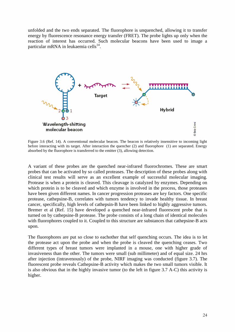
24
unfolded and the two ends separated. The fluorophore is unquenched, allowing it to transfer
energy by fluorescence resonance energy transfer (FRET). The probe lights up only when the
reaction of interest has occurred. Such molecular beacons have been used to image a
particular mRNA in leukaemia cells14
.
Figure 3.6 (Ref. 14). A conventional molecular beacon. The beacon is relatively insensitive to incoming light
before interacting with its target. After interaction the quencher (2) and fluorophore (1) are separated. Energy
absorbed by the fluorophore is transferred to the emitter (3), allowing detection.
A variant of these probes are the quenched near-infrared fluorochromes. These are smart
probes that can be activated by so called proteases. The description of these probes along with
clinical test results will serve as an excellent example of successful molecular imaging.
Protease is when a protein is cleaved. This cleavage is catalyzed by enzymes. Depending on
which protein is to be cleaved and which enzyme is involved in the process, those proteases
have been given different names. In cancer progression proteases are key factors. One specific
protease, cathepsine-B, correlates with tumors tendency to invade healthy tissue. In breast
cancer, specifically, high levels of cathepsin-B have been linked to highly aggressive tumors.
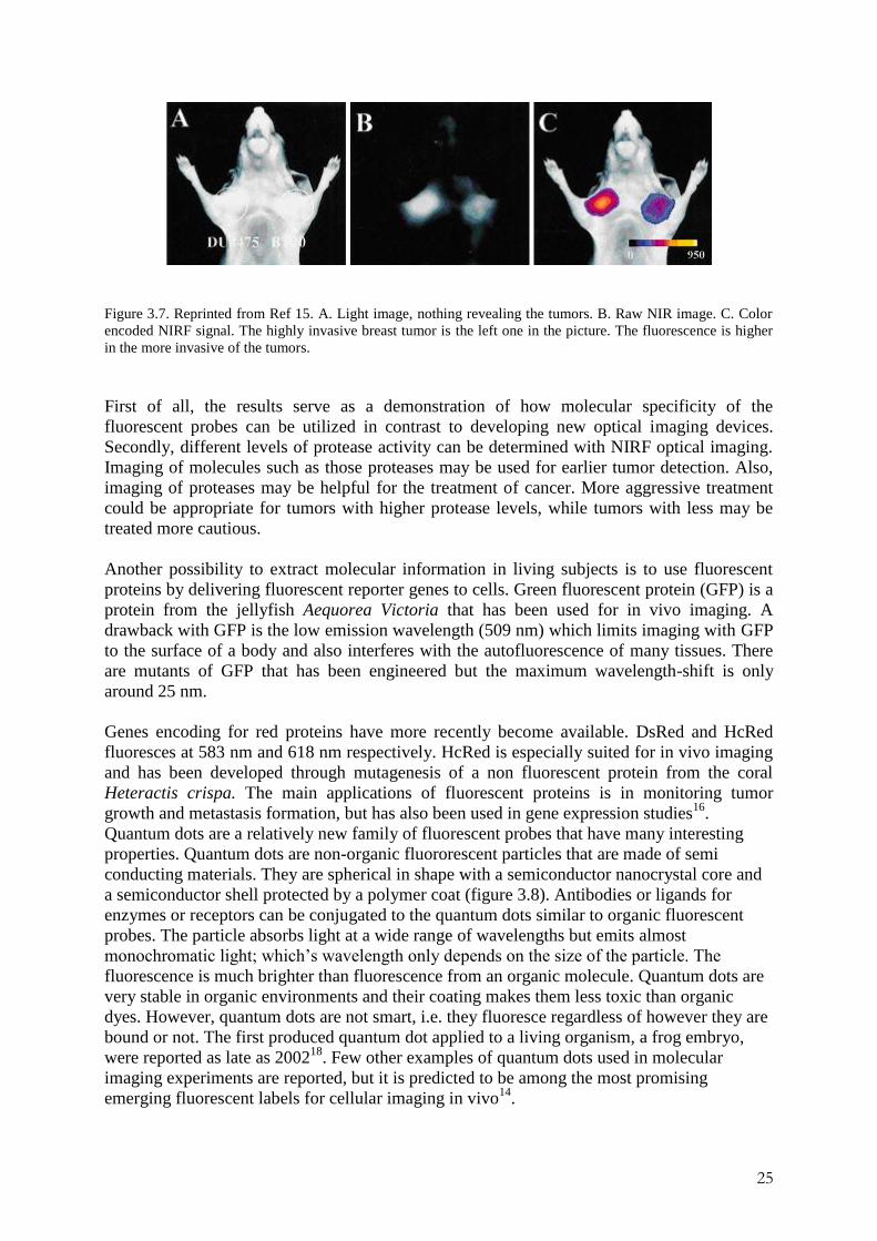
Bremer et al (Ref. 15) have developed a quenched near-infrared fluorescent probe that is
turned on by cathepsine-B protease. The probe consists of a long chain of identical molecules
with fluorophores coupled to it. Coupled to this structure are substances that cathepsine-B acts
upon.
The fluorophores are put so close to eachother that self quenching occurs. The idea is to let
the protease act upon the probe and when the probe is cleaved the quenching ceases. Two
different types of breast tumors were implanted in a mouse, one with higher grade of
invasiveness than the other. The tumors were small (sub millimeter) and of equal size. 24 hrs
after injection (intravenously) of the probe, NIRF imaging was conducted (figure 3.7). The
fluorescent probe reveals Cathepsine-B activity which makes the two small tumors visible. It
is also obvious that in the highly invasive tumor (to the left in figure 3.7 A-C) this activity is
higher.
25
Figure 3.7. Reprinted from Ref 15. A. Light image, nothing revealing the tumors. B. Raw NIR image. C. Color
encoded NIRF signal. The highly invasive breast tumor is the left one in the picture. The fluorescence is higher
in the more invasive of the tumors.
First of all, the results serve as a demonstration of how molecular specificity of the
fluorescent probes can be utilized in contrast to developing new optical imaging devices.
Secondly, different levels of protease activity can be determined with NIRF optical imaging.
Imaging of molecules such as those proteases may be used for earlier tumor detection. Also,
imaging of proteases may be helpful for the treatment of cancer. More aggressive treatment
could be appropriate for tumors with higher protease levels, while tumors with less may be
treated more cautious.
Another possibility to extract molecular information in living subjects is to use fluorescent
proteins by delivering fluorescent reporter genes to cells. Green fluorescent protein (GFP) is a
protein from the jellyfish Aequorea Victoria that has been used for in vivo imaging. A
drawback with GFP is the low emission wavelength (509 nm) which limits imaging with GFP
to the surface of a body and also interferes with the autofluorescence of many tissues. There
are mutants of GFP that has been engineered but the maximum wavelength-shift is only
around 25 nm.
Genes encoding for red proteins have more recently become available. DsRed and HcRed
fluoresces at 583 nm and 618 nm respectively. HcRed is especially suited for in vivo imaging
and has been developed through mutagenesis of a non fluorescent protein from the coral
Heteractis crispa. The main applications of fluorescent proteins is in monitoring tumor
growth and metastasis formation, but has also been used in gene expression studies16
.
Quantum dots are a relatively new family of fluorescent probes that have many interesting
properties. Quantum dots are non-organic fluororescent particles that are made of semi
conducting materials. They are spherical in shape with a semiconductor nanocrystal core and
a semiconductor shell protected by a polymer coat (figure 3.8). Antibodies or ligands for
enzymes or receptors can be conjugated to the quantum dots similar to organic fluorescent
probes. The particle absorbs light at a wide range of wavelengths but emits almost
monochromatic light; which‟s wavelength only depends on the size of the particle. The
fluorescence is much brighter than fluorescence from an organic molecule. Quantum dots are
very stable in organic environments and their coating makes them less toxic than organic
dyes. However, quantum dots are not smart, i.e. they fluoresce regardless of however they are
bound or not. The first produced quantum dot applied to a living organism, a frog embryo,
were reported as late as 200218
. Few other examples of quantum dots used in molecular
imaging experiments are reported, but it is predicted to be among the most promising
emerging fluorescent labels for cellular imaging in vivo14
.

26
Figure 3.8. (Modified from Ref 17). The spherical shape of a quantum dot.
3.2 Bioluminescence imaging
Bioluminescence imaging is an optical imaging technique that makes use of energy dependent
reactions as source for light emission, in contrast to fluorescence imaging, where light
emission is stimulated by absorbed photons. Unlike fluorescence imaging, there is only one
way of distributing probes, namely by delivering bioluminescent genes. Bioluminescence
imaging reminds of fluorescent reporter gene imaging (e.g imaging of GFP) but has an
advantage to this technique in that there is no intrinsic background. Since no excitation light is
needed no autofluorescence can be stimulated in the tissue. Alike GFP imaging the optical
reporter has been isolated from a light producing animals and plants.
3.2.1 Probes for bioluminescence imaging
The optical reporter in bioluminescence imaging is the Firefly luciferase gene. Inside a cell
this gene encodes for an enzyme called Firefly luciferase. This enzyme is converted into
luciferin by some chemical reactions, which emits photons when reacting with oxygen (figure
3.9).

27
Figure 3.9. (Ref 7). A bioluminescent reporter gene delivered to a cell. The reporter gene encodes for a light
emitting enzyme.
Firefly luciferin normally produces light at 562 nm but has in comparison with GFP been
modified to produce red-shifted emission spectrum.
Bioluminescence imaging has been used for tracking tumor cells, stem cells and bacteria as
well as for imaging gene expression16
.
Optical reporter gene imaging (i.e bioluminescence imaging and fluorescent reporter gene
imaging) are suitable for molecular imaging in small animals, but are less likely to be adapted
for clinical applications. The methods do neither allow absolute quantification of target signal.
It is often used to follow disease progression in the same animal over time which can be seen
in figure 3.10. For bioluminescence imaging the signal depends on ATPf (adenosine
triphosphate), 2O and depth.
f A phosphorylated nucleoside that supplies energy for many biochemical cellular processes.

28
Figure 3.10. An example of imaging with bioluminescence. The picture shows a prostate cancer tumor modified
with bioluminescent reporter genes. The growing of the cancer is imaged over time. The numbers below each
image shows the number of bioluminescent cells. Reprinted from Ref 16.
3.3 Future outlook
Optical molecular imaging is an interesting field of molecular imaging due to the many
advantages it provides: it is relatively cheap, non-radioactive and has many fields of
application. However, to improve the method further, advances has to be made within several
areas. The availability of more and further red-shifted probes must be improved. Such probes
are important to minimize absorption, scattering and autofluorescence. New, activable and
specific, probes must be engineered to extend the amount of targets possible to image.
Making the measurements more quantitative is another important issue for optical imaging.
This can be achieved with the use of photon migration theories. The lack of depth information
(three dimensional) imaging is also a problem associated with optical imaging.

29
4 Theory of light interaction in tissue
When light interacts with tissue several processes can occur during the propagation through
the medium. The various processes of absorption, scattering, reflectance, transmittance and
fluorescence can be utilized for characterizing biological tissue. The interaction processes
are strongly wavelength dependent. From an optical perspective, different types of tissue
can be distinguished by the size and the shape of the cell, the distribution of absorbing
substances, the scattering structures and any possible internal structure. Analyzing the
propagation of light in tissue can yield information about optical properties; absorption and
scattering coefficients μa and μs , and the scattering anisotropy factor or simply „„g-factor‟‟.
In section 4.1, the basic aspects of light-tissue interaction in simplified manner are
presented.
When working with strongly scattering media, as in the case of tissue optical studies, you
primarily have to deal with two problems, refered to as the forward problem and the
inverse problem. Solving these problems is the key to calculate the lights distibution and
the optical properties of the tissue23,24
.
The forward problem concerns the calculation of the energy density [ Jm-3
] of the laser
light in a certain position within the tissue, given that the optical absorption and scattering
properties are known. The unknown optial properties of the inverse problem can be derived
from measuring the distribution of reflected or transmitted light in the tissue25
.
The determination of the optical properties of tissue is a central part of tissue optics
because in order to solve the inverse problem, the forward problem has to be solved first26
.
In other words, the fundamental problem is to describe how light propagates through
biological tissue which consists of a large number of randomly distributed scattering
kernels. The kernels may consist of small regions with a refractive index differing from the
surrounding, as for example the mitochondria, cell membranes or even whole cells.
When both the forward and the inverse problem are solved, tissue optics can be a powerful
tool within medical research. When the light propagation is accurately modeled and the
scattering and absorption properties are quantified, tissue analysis can be used, for
example, for diagnostic27
purposes or for dose calculation28
during laser treatment. In
sections 4.2-4.3 this is further treated, along with different methods to model the
propagation of light.

30
4.1 Light-tissue interaction
4.1.1 Light
The electromagnatic radiation spectrum stretches from wavelength less than 10-13
m to
more than 105 m. The visible light is composed of a narrow band of wavelengths between
400-780 nm.
Fig. 4.1 The electromagnetic radiation spectrum.
The ultraviolet (UV) and the near infrared (NIR), bands are bordering this region. The
wavelength (λ) of light, assumed to be well known, can be stated as:
E
ch (7)
cv
(8)
where E is the quanta of light energy, v is the frequency and h is Planck‟s constant.
4.1.2 Absorption
Biological tissue contains different absorbing molecules, chromophores, which absorbs
energy in different wavelength regions. The absorption coefficient, μa [m-1
], describes the
probability of the tissue molecules to absorb photons energy per unit length. The light
absorption mainly depends on the type and the internal configuration of the molecules as
well as their concentration and distribution within the tissue. The absorbed energy can be
converted to heat, give rise to fluorescence or catalyze a photochemical reaction. Light in
the UV region, below 400 nm, is strongly absorbed due to high concentration of absorbing
molecules. Water, lipids and hemoglobin are the main absorbers in the visible and NIR
region. Water is a dominant chromophore of most tissue above 900 nm with a peak around
970 nm. A wavelength region between approximately 700 – 1300 nm , often referred to as
the optical window, is used for diagnostic and therapeutic purposes due to the deeper
penetration into the tissue in this region. In this region, the blood absorption has decreased
while the scattering coefficient is dominant25
.

31
4.1.3 Scattering
Light scattering is one of the most important processes that can occur during light
propagation inside tissue. There are different contributors to light scattering in tissue. When
the photon characteristics of light is applied, then light scattering is regarded on a
molecular level. Photons may give rise to excitation process followed by de-excitation to
either the initial state or to a higher/lower laying level. Relaxation to the initial state do not
cause net energy transfer to the media, this means that the scattered photon still have the
same wavelength as the incoming light (elastic scattering). However, relaxation to a
higher/lower laying level implies a net change in the potential energy of the molecule. If
the scattered photon has gained or lost energy a change in the wavelength has occurred (
Raman scattering).
Light scattering from microscopic tissue components is hardly influencing the resultant of
scattering characteristics. This is perceived at cellular and sub-cellular constituents, such as
the cell membrane, organelles and cytoplasm29
. The wave characteristics of light is almost
exclusively applied when treating light scattering at microscopic level. Thus, light
scattering is regarded as a process arising from spatial variations in refractive index. The
refractive index of tissues varies in a very complicated manner at a microscopic level.
Therefore a detailed description of the refractive index at this level is unfeasible. However,
some important conclusions regarding light scattering on a microscopic level can be drawn.
The main scattering features in tissue are the mitochondria30
and lipid vesicles (fat
droplets).
When applying the transport theory, a macroscopic refractive index is used due to the
complexity of the microscopic structure. The macroscopic refractive index is measured by
analyzing the Fresnel reflection from a tissue surface. The macroscopic refractive index of
most tissue types measured in this way are in the range 1.38 – 1.41 at 632.8 nm31
.
4.1.4 Anisotropy factor
The scattering is assumed to be symmetric which means that the scattering phase function
is a function of the scattering angle, such that p(s,s׳) = p(θ), where θ is the angle between
the incident and the scattered photon. It is further assumed that all photons have the same
energy.
The Henyey-Greenstein32
function is the analytical expression for the scattering phase
function that is often used for light transport in biological tissue:
23
2
2'
)cos21(2
)1()(),(
gg
gpssp
(4)
where g is the scattering anisotropy factor and is defined as g = <cosθ>.

32
4.2 Ligth propagation models – the forward problem
It is possible to model the light scattering by two theories: wave theory (Maxwell‟s
equations) or transport theory. The wave theory relies on solutions of the Maxwell
equations which can be solved numerically. If we are investigating scattering from
spherical particles, Mie theory is best suited33,34
, while T-matrix theory is the prime
candidate to particles of arbitrary shape38,39
. The optical properties are defined by the
complex dielectric constant, ε(r). The scattering and the absorption properties are
represented by Re{ε(r)} and Im{ε(r)} respectively. However, the variation of ε(r) on a
microscopic level is vastly complex. Therefore, the transport theory is better suited for
strongly scattering medium such as biological tissue.
In transport theory, the light propagation in tissue is treated as a stream of photons. Each
photon transports a quantum of energy. The transport of the photons energy can
mathematically be expressed by the radiative transport equation (RTE)35,36
.
The tissue is considered to be a homogeneous medium containing randomly distributed
absorption and scattering centres, simply characterized by three parameters: the absorption
and scattering coefficients, μa and μs, as well as the scattering anisotropy factor, g.
4.2.1 The transport equation
The radiative transport equation (RTE) has been very useful for calculating photon
transport in tissue37
.
The equation treats the changes in the radiance L( r,s,t ) [ Wm-2
sr-1
] which is the quantity
that describes the propagation of photon power per unit area and unit solid angel in the
direction s. The transport equation can be written as:
(1) where c [m/s] is the speed of light in the medium, μa[m
-1] the absorption coefficient, μs[m
-1]
the scattering coefficient, p(s,s׳) [-] the scattering phase function which gives the
probability of scattering from direction s ׳
into direction s and dω(s) that denotes an
infinitesimal solid angle in the direction s23
.
The change in number of photons, at position r, in direction s at time t, is represented in the
left-side of equation (1). The first two terms of the right-side describe the amount of
escaped photons over the volume boundary, and due to absorption and scattering into other
directions, the third term describes gained photons due to scattering from other directions
into s and the last term (Q) is the gain due to a light source inside the volume element.
The radiance can be stated as:

33
L( r,s,t) = N( r,s,t)
2hc (2)
where N(r,s,t) [m-1
sr-1
] is the photon distribution function which is the volume density of
photons per unit solid angle.
Another important quantity is the fluence rate Φ [W/m2], which describes the
power incident on a volume element per surface area:
4
)(),,(),( sdtsrLtr (3)
4.2.2 Solving the transport equation
Analytical solutions to the RTE are available only for a few special cases. On the other
hand, there are various of methods based on approximation such as diffusion
approximation. In practice, numerical methods such as Adding-Doubling38
or Monte
Carlo39
simulations are the most widely used. .
4.2.3 The Monte Carlo method
The conventional Monte Carlo method is frequently used as a model for simulating light
transport in tissue. It is based on building a stochastic model where individual photons
pathways are traced randomly. The scattering and absorption events are governed by the
probabilities given by μs and μa as well as the phase function p(s,s׳).
One drawback with Monte Carlo simulations is the requirement of significant computation
time if high precision and accuracy is wanted. It is also difficult to get good statistics if the
point of interest is located far from the point of entry and the coefficients for absorption
and scattering are high. However the method is a flexible and helpful tool for modelling
and has no limitations concerning boundary conditions or spatial localization of
inhomogeneities in the tissue.
The optical properties for each layer is defined before the simulation is started. Properties
required are the absorption coefficient μa, the scattering coefficient μs , the anisotropy
factor g, the refractive index n and thickness d of the sample. It is also necessary to define
optical properties for the top ambient medium (most often air) and bottom ambient medium
(if this is existent).
A number of photons, or rather photon packages, are launched into the medium. The
number of photons used depends on which problem the simulation is supposed to solve.
The reason for launching many photons at a time, as a packages, is that it improves the
efficiency since normally only one photon follows the selected pathway. The packet starts
off with a weight w set to 1. In several steps it has the possibility of being propagated
undisturbed, absorbed, scattered, reflected internally or transmitted out of the tissue.
34
The simulation continues until the photon is either absorbed or exits the tissue. If it escapes
the reflectance and transmission are recorded, and if it is absorbed the position where this
took place is recorded. The final results from the simulation are fluence, transmittance,
reflectance and photon absorption.
The program Monte Carlo simulation for Multi-Layered media, MCML, by Jacques and
Wang39,40
, has become somewhat of a standard in the field of tissue optics.
An adaptation to time-resolved data and more complex geometries was implemented by
Berg41
, but the photon propagation routines are the same for all subsequent versions of the
program. Various Monte Carlo models were developed to simulate fluorescence spectra
from layered tissues42
. A basic approach to describe fluorescence within transport theory is
to regard the propagation of the excitation light and the emission light as two different
problems, and find a way to handle the transition of excitation light to fluorescence light.
4.3 The inverse problem
One of the more important aspects of the inverse problem is the number of the unknowns.
There are spatial parameters, optical properties and also geometrical parameters, such as
the thickness of the layer as unknowns. If the medium is homogeneous, the number of
unknowns is reduced to the number of optical properties. Thus, the formulation to the
inverse problem in such case is to find the optical properties μa, μs, and g, where the
propagating light is measured.
There are two-parameters methods where both µs‟ = µs(1-g) and µa are unknown and three
parameters methods, where all three µs, µa and g are unknown such as the integrating sphere
method26
, and the medium is assumed homogeneous.
4.3.1 Two-parameters methods
Two-parameters methods are based on measurements of the diffuse reflectance or
transmittance from the medium. The measurements can be spatially resolved, time resolved
or frequency resolved (see Fig. 4.2). Spatially resolved measurements are based on
continuous wave (Cw) light. With this method, as well as with the time-resolved technique,
it is possible to make measurements in vivo. The major advantage with the spatially
resolved technique is that it can be performed with cheap light sources (e.g. lamps or diode
lasers) and detectors (e.g. photodiodes). A drawback is that the method is sensitive to
inhomogeneities in the medium43
.

35
(a)
(b)
(c) Fig.4.2 The principles of three two-parameters techniques to obtain μs
‟ and μa
, are schematically illustrated:
(a) Cw spatially resolved reflectance measurement; (b) time resolved measurement and (c) frequency domain
measurement where the phase shift and the modulation depth = BC/AD is measured.

36
4.3.2 The integrating sphere method
This method is used for measuring three parameters: collimated transmittance, Icol ,total
transmittance, Tmeas, and diffuse reflectance, Rmeas. The optical parameters of the tissue are
deduced from these measurements using different theoretical expressions and numerical
methods to obtain µs ,µa and g.
The first parameter Icol is measured by letting a beam of light pass through a tissue sample and
only measure the light that has not been scattered inside the tissue. This gives us the total
interaction coefficient, µt,meas =µa+µs. The total interaction coefficient can be recognised from
the Beer-Lambert‟s formula, stating that the intensity of a beam passing straight through a
sample with the thickness d decays exponentially:
).exp(0 dII tcol (5)
To measure the diffuse reflectance Rmeas and the total transmittance, Tmeas, a so called
integrating sphere is used. Measuring T, the tissue sample is placed in front of the sphere. The
light passes through the sample, is scattered and registered by a detector inside the sphere.
The inside walls in the sphere are covered by a material that reflects the light in all directions.
Measuring R the sample is placed in the end of the integrating sphere. The reflected light is
collected in the sphere and detected.
Converting R,T and µt, to µa , µs and g are the solutions of an inverse problem. Polynomial
regression is often recommended method. It is an iterative method which approximate the
solutions to the forward model with 3-dimensional polynomials. A Monte Carlo generated
database, producing maps of RMC and TMC as functions of µa , µs and g are used. An
expansion of Chebychev polynomials is used to fit Monte Carlo generated data, yielding
Rcheb(µa,µs,g) and Tcheb(µa,µs,g) (see figure 4.3). The optical properties are determined by
finding the common roots of the new polynomials:
meastsasa
meassachebsa
meassachebsa
gH
TgTgG
RgRgF
,),,(
),,(),,(
),,(),,(
(6)
The common roots is solved by setting the polynomial equal to zero which can be done by a
Newton-Raphson solver.
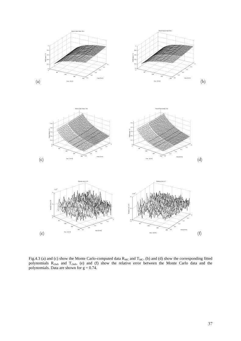
37
(a)
0
0.1
0.2
0.3
0.4
0.5
0
50
100
150
200
0
0.2
0.4
0.6
0.8
1
mua [1/cm]
Monte Carlo Data: Rmc
mus [1/cm]
Refle
cta
nce
%
0
0.1
0.2
0.3
0.4
0.5
0
50
100
150
200
0
0.2
0.4
0.6
0.8
1
mua [1/cm]
Fitted Polynomials Rmc
mus [1/cm]
Refle
cta
nce
%
(b)
(c)
0
0.1
0.2
0.3
0.4
0.5
0
50
100
150
200
0
0.1
0.2
0.3
0.4
0.5
mua [1/cm]
Monte Carlo Data: Tmc
mus [1/cm]
Tra
nsm
itta
nce
%
0
0.1
0.2
0.3
0.4
0.5
0
50
100
150
200
0
0.1
0.2
0.3
0.4
0.5
mua [1/cm]
Fitted Polynomials Tmc
mus [1/cm]
Refle
cta
nce
%
(d)
(e)
0
0.1
0.2
0.3
0.4
0.5
0
50
100
150
200
-5
0
5
x 10-3
mua [1/cm]
Relative error in R
mus [1/cm]
Rela
tive
err
or
in R
0
0.1
0.2
0.3
0.4
0.5
0
50
100
150
200
-5
0
5
x 10-3
mua [1/cm]
Relative error in T
mus [1/cm]
Rela
tive
err
or
in R
(f)
Fig.4.3 (a) and (c) show the Monte Carlo-computed data RMC and TMC. (b) and (d) show the corresponding fitted
polynomials Rcheb and Tcheb. (e) and (f) show the relative error between the Monte Carlo data and the
polynomials. Data are shown for g = 0.74.

38
5 Imaging deep interior tissue volumes
Much effort has been devoted to detect and image heterogeneities in biological tissues with
diffuse near-infrared (NIR) light. Several investigators have been interested in the
determination of the absorption and scattering coefficients in tissue and tissue-like
phantoms. To enhance the specificity and sensitivity in tumor detection, fluorescent contrast
agents have been frequently used. Several reconstruction algorithms have been published
that attempt to recover the distribution of a fluorophore in a tissue volume given a set of
measurements on the tissue surface. Fully three-dimensional reconstruction methods are
being developed by some groups. Most commonly these are based on diffusion theory as the
forward model44,45
, but an algorithm based on discrete-ordinates solution of the transport
equation has also been proposed46
. Many combinations of light source and detection points
are needed for full reconstruction, which implies high complexity of both the
instrumentation and the reconstruction algorithm. A simpler approach has been suggested by
some authors, based on the approximation that the tissue can be regarded as a semi-infinite
volume with fluorescing lesions at some depth from the surface. Stasic et al. presented a
method based on the diffusion equation for a two-layer medium and spatially resolved
measurements of both diffuse reflectance and fluorescence47
. This method was successful in
recovering the absorption and reduced scattering coefficients (µa and µs', respectively) of
both layers, as well as the fluorophore concentration and depth of the layer. However,
recovery of all parameters was limited to a depth of about 3 mm, and determination of the
depth itself proved to be difficult for larger depths due to model coupling between depth,
fluorophore concentration and tissue absorption. Eidsath et al. have described a method
based on image fluorometry using a CCD camera48
. Using a random-walk model, good
accuracy of the determined depth was demonstrated for point-like fluorescing lesions.

39
6. Analysis of a fluorescence spectrum for determination of depth
The goal of the experimental part of this work is to develop a method for estimating the depth
of fluorescent lesions in tissue. The method has been simulated on computer and compared
with experimental results for validation.
The idea is to make use of changes in the spectral shape of the fluorescent light in order to
reveal information about the depth. The changes are induced by tissue absorption and
scattering as the light propagates from the fluorophore towards the surface of the body.
Making use of the spectral properties of the fluorescent light is an alternative approach to
those mentioned in section 5 (depth information) that not yet seem to have been investigated.
To explain the idea, we consider a typical absorption/scattering spectrum of mammalian tissue
(figure 6.1).
0
0.1
0.2
0.3
0.4
600 700 800 900 1000
Wavelength (nm)
Ab
so
rptio
n (
cm
-1)
0
5
10
15
20
Re
du
ce
d s
ca
tte
rin
g (
cm
-1)
#1
#2
#3
#4
#5
#6
Mean Scattering
Figure 6.1. Optical properties of six different types of breast tissue
19. The absorption spectra represent fitted data
rather than actual measurements. The reduced scattering spectra were fitted to a power law. Only the mean
spectrum is shown for scattering to avoid cluttering in the graph. The error bar indicates the standard deviation.

40
At around 600 nm a marked decrease in absorption can be observed. This is the beginning of
the optical window. From 800 nm the absorption starts to increase slightly again, because of
fat absorption and subsequently runs up just above 900 nm. The strong absorption around 970
nm is due to water in the tissue that has an absorption peak at this wavelength. Fluorescence
light propagating through tissue with constant absorption and scattering would not have a
change in the spectrum. The intensity of the fluorescence would decrease for longer pathways
but the shape remains the same. However, a fluorophore whose emission spectrum covers a
range where the absorption has a gradient (as around 600nm or above 900 nm) will have its
fluorescence light altered in shape. Some of the emissions wavelengths will be absorbed more
than others. This effect will be greater the longer the pathway through the tissue is. Our
approach is to investigate whether the depth of a fluorophore embedded in tissue can be
revealed from forming a ratio between two parts of the emission spectrum, affected by
differently strong absorption. This is described by the simple formula:
)(
)(
2
1
With data like those in figure 6.1 as template, computer simulations along with experimental
phantom measurements were going to be made for different depths of fluorescent lesions in
order to investigate whether the spectral changes can be used to reveal the depth. In the
simulations )( represents the probability of detecting a photon of wavelength at the
surface of the sample, and in the experimental measurements )( is the measured intensity at
the surface of the phantom of the detected light at wavelength .
In addition to absorption - scattering and the measurement geometry will affect the
deformation of the fluorescent spectra. This is also taken into account in the simulations.

41
7 Material and method
Performing simulations of a fluorescent lesion on different depths in tissue is rather
unproblematic. The programs available request information about the optical properties of the
tissue, at the wavelength of the excitation and fluorescence light along with the shape and size
of the sample. Most questions raised during this work therefore regard the practical part of the
experiments, i.e. the phantom measurements.
Before and during the measurements and simulations the following issues are necessary to be
considered:
Which tissue optical properties that should be used as model for the simulations and
phantom measurements
The best possible wavelength range for this type of measurements
Choosing of fluorescent dye
Excitation source
Type of phantom
Which detector to use
Method of simulation
Convenient quotient
At the department of Atom Physics in Lund, previous measurements of breast tissue have
been made. The access to those and the fact that optical imaging and breast cancer research
often are linked together makes it appropriate to use these data. The absorption/scattering
spectra of six different types of breast tissue are shown in figure 6.1. A fluorescent dye in this,
red, spectral region seldom fluoresces over a bandwidth greater than 200 nm42
. In the graph
shown in figure 5.1 there are two regions of non-uniform absorption likely to give rise to
measurable changes in the relative spectral intensity of the fluorescence light. These two
regions where the absorption changes dramatically are as mentioned earlier around 600 nm
and just above 900nm. Since no fluorescence will cover them both, one has to be chosen. One
advantage with the latter is that the absorption is low for shorter wavelengths than 900nm,
where the dye will have its absorption maximum. This implies greater penetration depth for
the excitation light. A fluorophore that emits at, for example, 620nm has its absorption peak
around 560 nm. At this wavelength the tissue is much less transparent and the light exciting
the dye would not reach deep into the tissue. Another advantage is that the dominant
absorbers in tissue at wavelengths above 900 nm are water and lipids, which facilitate the
preparation of a liquid phantom with well agreeing optical tissue properties for the region of
interest. Below 600 nm, on the contrary, the absorption is caused by deoxygenated and
oxygenated hemoglobin. With this motivation the region above 900nm was decided to be
used for the experiments. Next a fluorophore emitting light in this spectral area along with a
suitable excitation source and detector had to be found. The best available excitation source in
the NIR region was a Ti:Sapphire laser at 780 nm. Having decided the excitation laser light
source reduced the amount of usable fluorescent dyes severely. The excitation wavelength of

42
the laser and the absorption maximum should match in order to get as much light as possible
out from the dye. Two fluorescent dyes remained that had absorption maximum around
780nm and could be used for lasing up to 1000nm. Those were IR-140 (Exciton, USA) and
LC9280 (Lambda Physik, Germany). Since laser dyes in the NIR region have very poor
solubility in water and poor quantum yield we decided to try them both to increase the
chances of good results.
During the experiments three different detectors were tried out. All but one showed way to
high signal-to-noise ratio of the detected fluorescence at the surface of the phantom. The first
one investigated was a STREAK camera operating in the NIR region which not only provides
spectral but also temporal information. The temporal information was meant to be compared
with the spectral to demonstrate advantages of using spectrally resolved measurements or,
alternatively, to gain additional information about the depth. The STREAK camera had far too
low sensitivity and required hours of detection time already at relatively shallow tumor depth.
The second detector was a non-cooled spectrometer (Princeton Instruments) with fairly good
sensitivity in the NIR spectrum. With this detector the detection time was reduced but the
signal-to-noise ratio was higher than what could be accepted. The final detector was far more
sensitive for the measurements than the other two. This detector (HoloSpec f/1.8i, Kaiser
Optical Systems, USA) consists of a spectrometer and a cooled CCD camera coupled
together. It is normally used for RAMAN spectroscopy in the region around 900nm.
(We use Monte Carlo simulations to compute fluorescence spectra. The Monte Carlo code
was developed earlier and is especially suited for simulating fluorescence from layered
tissue42
.)
7.1 MC-simulations
For experimental validation we performed Monte Carlo simulations with optical properties
similar to phantoms, whose optical properties were measured independently using an
integrating-sphere method (sections 7.2.1 and 7.2.2 below).
The amount of traced photons were 5105. All other values (e.g. excitation wavelength,
distance between detection point and excitation point) were in correspondence with the
experimental phantom measurements.
7.2 Tissue phantom
Measurements were performed on a model that consisted of three parts: the upper and the
lower parts, where the liquid phantom material was stored, and in between those a 1 mm thick
layer, where the same liquid with some added fluorescent dye was kept see figure 7.1. The
walls of the model was made of two plastic cylinders (=7cm). In the bottom of each
cylinder, thin plastic film was attached, for separating the liquids without affecting the light
when propagating between them. The third layer was constructed by placing the two cylinders
on top of each other, with their film–covered surfaces facing each other and isolating the
small resulting volume. Liquid could easily be added and removed to the upper part so the
height of the surface could be varied (i.e the depth of the fluorophore), see figure 7.1.

43
Excitation laser
780 nm Spectrometer
Variable depth
Intralipid solution
Intralipid solution
Inralipid solution + fluorophore
5 mm
Diameter= 7cm
Plastic wall
Plastic film
Figure 7.1. Water based tissue phantom with variable depth of the fluorescent lesion.
7.2.1 Preparing the liquid phantom
The liquid tissue phantom was prepared by mixing 21 parts of water with 1 part 20%-Intra
lipid solution (Fresenius Kabi AG) which corresponds to a lipid concentration of 0.91%. To
increase the absorption a concentration of 2.3 l ink/liter was added to the lipid mix. Figure
A.1 (Appendix 1) describes how the overall absorption varies as a function of different
amount of added ink. 2.3 l ink/liter puts the absorption on a level very proximate to the
template values. The black ink was taken from a copying machine. Resulting absorption and
scattering properties were measured with an integrating sphere. To translate R and T to µa , µs
and µs‟ a Monte Carlo database was generated specifically designed for this application
(section 4.3.2). The generated database covered an interval of 1 to 200 cm-1
and 0.01-0.4 cm-1
for µs‟ and µa respectively.
The absorption and scattering properties of the liquid as a function of wavelength are
presented in figure 8.3 below. The prepared Intra lipid solution simulates healthy tissue and
was kept in the upper and the lower part of the beacon, see figure 7.1.
7.2.2 Fluorescent layer
For the intermediate layer of the phantom a solution with the same optical properties as the
rest of the phantom, but with fluorescent properties had to be prepared. This was achieved
simply by adding a small amount of dye solved in ethanol to the 0.91% Intra lipid solution.
The amount of dye solution should be as high as possible in order to maximize the
fluorescence but low enough not to affect the optical properties in the spectral region where
the measurement were going to be made. The main concern was that the dye would absorb
above 870 nm and in such manner disturb the measurements by reabsorbing its fluorescence.
By pointwise integrating sphere measurements, using interference filter, the highest possible

44
concentration was found. Such measurements were made for the two available dyes, IR-140
and LC9280. It appeared to be possible to add more than twice as much LC9280 to the
solution as IR-140. However, the strength of the fluorescence were almost similar for the two
dyes so nothing was gained by the possibility to use the higher concentration LC9280
solution. On the contrary, the higher amount of alcoholic solution was more of a drawback
since the intralipid showed tendencies to aggregate rather quickly. The conclusion was that
IR-140 was a more efficient dye than LC9280 and was therefore used for the rest of the
measurements.
In appendix 2 pointwise integrating sphere measurements of dye/Intra lipid mix is
presented.
7.3 Experimental phantom measurement
Figure 7.2 illustrates the experimental arrangement used for the measurements. Two fibers
(Super Guide, = 400 m, NA = 0.22; Fiberguide Industries) were led into the upper part of
the phantom, one for the excitation light and one for detection of fluorescence. The light from
the laser passed an interference filter of 780 nm (filter 1) before entering the fiber and had an
intensity of approximately 10mW when illuminating the surface of the phantom. The
detection light was filtered with long-pass filter (RG 780; Schott Glass Technologies, Inc.),
filter 2, to ensure no back scattered light from the excitation light was mixed with the
fluorescence light. The light was led into a holographic imaging spectrograph (HoloSpec
f/1.8i; Kaiser Optical Systems, Inc.) with an interference grating efficacious from 815nm to
960nm. A nitrogen-cooled CCD camera (LN/CCD-1024-EERB/1; Princeton Instruments,
Inc.) recorded the spectral image. The CCD was coupled to a detector controller (Princeton
Instruments, Inc) and was set to operate at a temperature of -110C. To view the resulting
spectrum and to communicate with the CCD the program WinSpec/32 version 2.3.3.3 (Roper
Scientific, Inc.) was used.
(The excitation light was led out from the oscillator of the tera-watt laser at Lund Laser
Centre. This is a pulsed Ti:Sapphire laser pumped with an Ar+ -laser. After passing the
780nm interference filter the pulse was strongly broadened, but in our experiment temporal
information was not of interest.)

45
Figure 7.2 Schematic diagram of the set-up for spectroscopy measurements.
During measurements the height of the liquid tissue material was increased by 1.14 mm at a
time, starting from 0mm to 1.14cm. Spectra were acquired in the wavelength range of 815-
960 nm.

46
8 Results
The optical properties of the Intralipid phantom as determined by the integrating sphere
method (shown in fig. 8.1) were used as input for the Monte Carlo simulations.
0
0.1
0.2
0.3
0.4
0.5
750 800 850 900 950
Wavelength (nm)
Ab
so
rptio
n (
cm
-1)
0
5
10
15
Re
du
ce
d s
ca
tte
rin
g (
cm
-1)
Absorption
Scattering
IR140 Fluo. (a.u.)
Figure 8.1. The optical properties of the Intra lipid phantom. The intrinsic fluorescence spectrum of IR-140 is
also shown.
In this case g was around 0.65 over the wavelength range. The measured fluorescence spectra
at different depths are presented in figure 6.4, which shows the shift of the spectrum as the
depth increases.

47
0
0.25
0.5
0.75
1
825 850 875 900 925
Wavelength (nm)
Inte
nsity (
no
rma
lize
d)
2 mm
6 mm
10 mm
Figure 8.2 Measured (normalized) fluorscence spectra for different depths of the layer with fluorescing IR 140:
2, 6 and 10 mm.
In the Monte Carlo simulations, the highest value of the ratio was obtained with 1=815 nm
and 2=960 nm. However, due to the low fluorescence signal at long wavelengths we had to
use a lower 2 to obtain a good signal-to-noise ratio from the measurements. Due to influence
of autofluorescence when the excitation and detection fibers were close together we used a
fiber distance of 5 mm. Therefore, the measurement was limited to depths larger than about 1
mm. In figure 6.5 we present (normalized to the value at d=2 mm) as a function of d for
1=886 nm and 2=922 nm.

48
Figure 8.3. The ratio shown for 1 = 886 nm and 2 = 922 nm, as a function of the depth d, normalized to the
value for d=2. Results from both measurements on the Intralipid phantom and the Monte Carlo simulations are
shown.

49
9 Discussion and Conclusions
The results from the Monte Carlo simulations show that the ratio (1,2) indeed is a useful
indicator of the depth of a fluorescing lesion for the right combinations of wavelengths 1 and
2. The results from the phantom measurements corroborate the simulations and show that the
method is practically feasible using a relatively simple experimental set-up. In the case of the
Intralipid phantom we utilize the difference in water absorption that has a maximum
absorption at 970 nm. Here we used 2=922 nm, although a longer wavelength would have
given a higher ratio , but we were limited to about 930 nm by the spectrometer and the fact
that the fluorescence spectrum for IR-140 drops to low intensity for longer wavelengths (as
can be seen in figure 6.3). It is worth to mention that the amount of dyes fluorescing above
850 nm is rather limited. An alternative to IR-140 and LC9280, that fluoresce farther up in the
NIR region, but still have good absorption around 780 nm would be ideal. A more careful
analysis of the results show that we were able to recover the depth of the fluorescing layer
from the experimental data with an accuracy of 0.6 mm42
.
A better choice of wavelengths would be (1,2)=(875 nm,935 nm). With this pair of
wavelengths it has been shown in ref 50, that the depth can be recovered with good accuracy
and small dependence on variations in breast tissue from one person to another. This study,
however, is not conducted within this master thesis. To change region to the slope at 600-650
nm could also be an interesting idea.
With the present method, we envision a potential application based on a probe delivering
excitation light and at the same time detecting the fluorescence light by means of relatively
simple photodetectors and wavelength-selecting filters. The operator would manually scan the
probe across the tissue and information would be presented in the form of an indicator of
fluorescence intensity and the estimated depth of the fluorophore. We also consider our
method very promising in terms of providing depth information for image fluorometry and
molecular imaging, as a means to resolve the fluorophore distribution in three dimensions22
.

50
Acknowledgements
We would like to thank our supervisors, Jenny Svensson and Stefan Andersson-Engels, for
their guidance and encouragement, making this thesis possible. We would also like to express
our sincere gratitude to Johannes Swartling, for his support and work with the published
article, Christoffer Abrahamsson, for technical help during the experimental measurements
and Nazila Yavari for her engagement in needed situations.
Finally, we would like to thank our families and friends for all backing support.
Khaled Terike and Daniel Bengtsson

51
References
1. Tarik F. Massoud, Sanjiv S. Gambhir,”Molecular imaging in living subjects: seeing
fundamental biological processes in a new light,” Genes and development 17, 545-580,
(2003).
2. Bogdanov A, Weissleder R., “The development of in vivo imaging systems to study gene
expression,” Trends Biotechnol 16,5-10, (1998).
3. Christoph Bremer, Ralph Weissleder, “In vivo imaging of gene expression: MR and optical
technologies,” Acad Radiol 8,15-23, (2001).
4. Robert F. Service, “New probes open windows on gene expression, and more,” Science
280, 15 may (1998).
5. Roush, W., “Antisence Aims for a Renaissance,” Science 276, 1192-1193, (1997)
6. Bremer C, Bredow S, Mahmood U, Weissleder R, Tung C-H, “Optical imaging of matrix
metalloproteinase-2 activity in tumors: feasibility study in a mouse model,” Radiology
221,523-529, (2001).
7. Crump institute for molecular imaging, “Lecture on Molecular Imaging”,
http://laxmi.nuc.ucla.edu:8248/M248_04/syllabus.html (2004).
8. Weissleder R, “Scaling down imaging: Molecular mapping of cancer in mice,” Nat. Rev.
Cancer 2, 11-18, (2002).
9. Ching-Hsuan Tung et al., “In vivo imaging of proteolytic enzyme activity using a novel
molecular reporter,” Cancer research 60, 4953-4958, September (2000).
10. Molecular probes, Inc., Haugland, R.P. , “Molecular Probes Handbook for Fluorescent
Probes and Research Chemicals, 6th Edition” http://www.probes.com (1996).
11. Imaging research, Inc., “Fluorescence imaging,”
http://www.imagingresearch.com/applications/Fluorescence.asp (2004).
12. Brackmann, U. ”Lambdachrome laser dyes,” Lambda Physik, Göttingen 2000 (3rd
edition)
13. Lin et al, "Novel Near-Infrared Cyanine Fluorochromes: synthesis, Properties, and
Bioconjugation," Biocon Chem 13, 605-610, (2002).
14. Mitchell, P, “Turning the spotlight on cellular imaging,” Nat Biotechnol 19,1013-1017,
(2001).

52
15. Bremer et al, “Imaging of Differential Protease Expression in Breast Cancers for
Detection of Aggressive Tumor Phenotypes,” Radiology 222,814-818, (2002).
16. Weissleder, R. Ntziachristos, V. “Shedding light onto live molecular targets,” Nature
medicine 9(1), 123-128, January (2003).
17. Evident Technologies, Inc. “Quantum dots explained,” http://www.evidenttech.com/qdot-definition/quantum-dot-about.php
18. Benoit Dubertret et al.’’ In Vivo Imaging of Quantum Dots Encapsulated in Phospholipid Micelles,’’ Science vol 298, 29 november 2002 1759-1762
19. A. Pifferi, J. Swartling, E. Chikoidze, A. Torricelli, P. Taroni, A. Bassi, S. Andersson-Engels, and R. Cubeddu, “Spectroscopic time-resolved diffuse reflectance and transmittance 20. Molecular probes, Inc., “Molecular Probes Handbook for Fluorescent Probes and Research Chemicals,” http://www.probes.com/handbook/figures/0665.html 21. Swartling et al, “Fluorescence spectra provide information on the depth of fluorescent lesions in tissue”
22. C. Bremer, V. Ntziachristos, R. Weissleder, “Optical-based molecular imaging: contrast agents and potential medical applications,” Eur. Radiol. 13, 231-243 (2003)
23. A. Ishimaru, Wave propagation and scattering in random media (Academic press, New York, 1978). 24. K. M. Case and P. F. Zweifel, Linear transport theory (Addison-Wesley Publishing Co. 1967). 25. W. F. Cheong, S. A. Prahl, and A. J. Welch, "A review of the optical properties of biological tissues," IEEE J. Quant. Electr. 26, 2166-2185 (1990). 26. J.Swartling, Biomedical and atmospheric applications of optical spectroscopy scattering media, (2002). Ph.D. Thesis, Lund Institute Technology, Lund, Sweden. 27. R. Splinter, R. H. Svenson, L. Littman, J. R. Tuntelder, C. H. Chuang, G. P. Tatsis, and M. Thompson, "Optical properties of normal, diseased, and laser photocoagulated myocardium at the Nd:YAG wavelength," Lasers Surg. Med. 11, 117-124 (1991).
28. R. Berg, ’’Laser-based cancer diagnostics and therapy- Tissue optics considerations’’ (1995). Ph. D. Thesis, Lund Institute of Technology, Lund, Sweden. 29. A. M. K. Enejder, ’’Light scattering and absorption in tissue- models and measurements,’’ (1997). Ph.D. Thesis, Lund Institute of Technology, Lund, Sweden. 30. B. Deauvoit, S. M. Evans, T. W. Jenkins, E. E. Miller, nad B. Chance, ’’ Correlation between the light scattering and the mitochondrial content of normal tissues and transplantable rodent tumors,’’ Anal. Biochem. 226, 167-174 (1995). 31. F. B. Bolin, L.E. Preuss, R. C. Tayler, and R. J. Ference, ’’ Refractive index of some mammalian tissue using a fiber optic cladding method,’’ Appl. Opt. 28, 2297-2303 (1998).

53
32. L. G. Henyey and J. L. Greenstein, ’’ Diffuse Radiation in the galaxy,’’ Astrophys. J. 93, 73-83 (1941). 33. C. F. Bohren and D. R. Huffman, Absorption and scattering of light by small particles (John Wiley & Sons, Inc. New York, 1983). 34. H. C. van de Hulst, Light scattering by small particles (Wiley, New York, 1957). 35. A. Ishimaru, Wave propagation and scattering in random media (Academic press, New York, 1978). 36. K. M. Case and P. F. Zweifel, Linear transport theory (Addison-Wesley Publishing Co. 1967).
37. K. M. Case, "Elementary solutions of the transport equation and their applications,"
Annals of Physics 9, 1-23 (1960).
38. S. A. Prahl, M. J. C. van Gemert, and A. J. Welch, "Determining the optical properties of
turbid media by using the adding-doubling method," Appl. Opt. 32, 559-568 (1993).
39. S. A. Prahl, M. Keijzer, S. L. Jacques and A. J.Welch, A Monte Carlo Model of Light Propagation in Tissue, SPIE Institute Series Vol IS 5, 1989
40. L. Wang and S. L. Jacques, Monte Carlo Modeling of Light Transport in Multi-layeredTissues in Standard C, 1992
41. R. Berg, ’’Laser-based cancer diagnostics and therapy- Tissue optics considerations’’ (1995). Ph. D. Thesis, Lund Institute of Technology, Lund, Sweden. 42. J. Swartling, A.Pifferi, A:M:K:Enejder, and S.Andersson_Engels, ’’Accelerated Monte Carlo model to simulate fluorescence spectra from layered tissues,’’ Journal of the Optical Society of America, in press (2002). 43. Daniel J. Hawrysz and Eva M. Sevick-Muraka, ’’ Development Toward Diagnostic Breast Cancer Imaging Using Near_Infrared Optical Measurenents and Fluorescent Contrast Agents’’. Neoplasia, Vol. 2. No. 5, September- October, 2000, pp. 388-417. 44. M.J. Eppstein, D.J. Hawrysz, A. Godavarty, and E.M. Sevick-Muraca, “Three-dimensional, Bayesian image reconstruction from sparse and noisy data sets: near-infrared fluorescence tomography,” Proc.Natl.Acad.Sci. 99, 9619-9624 (2002) 45. A.B. Milstein, S. Oh, K.J. Webb, C.A. Bouman, Q. Zhang, D.A. Boas, and R.P. Millane, “Fluorescence optical diffusion tomography,” Appl.Opt. 42, 3081-3094 (2004) 46. A. D. Klose, A. H. Hielscher, “Fluorescence tomography with simulated data based on the equation of radiative transfer,” Opt. Lett. 28, 1019-1021 (2003) 47. D. Stasic, T.J. Farrell, and M.S. Patterson, “The use of spatially-resolved fluorescence and reflectance to determine interface depth in layered fluorophore distributions,” Phys.Med.Biol. 48, 3459-3474 (2003)

54
48. A. Eidsath, V. Chernomordik, A.H. Gandjbakhche, P. Smith, and A. Russo, “Three-dimensional localization of fluorescent masses deeply embedded in tissue,” Phys.Med.Biol. 47, 4079-4092 (2002) 49. Pifferi, A. Swartling, J. Chikoidze, E. Torricelli, A. Taroni, P. Bassi, A. Andersson-Engels, S. and Cubeddu, R. “Spectroscopic time-resolved diffuse reflectance and 50. Swartling, J. Svensson, J. Bengtsson, D. Terike, K. Andersson-Engels, S. “Fluorescence spectra provide information on the depth of fluorescent lesions in tissue”

55
Appendix 1
Absorption of the phantom liquid as a function of added ink
Five samples with different concentration of ink were prepared and absorption measurements
were performed with an integrating sphere. The measurements were conducted by first
preparing two premix solutions, one of ink and one of pure 0,91% Intralipid solution. These
two premixes were mixed in five different amounts that were separately measured with the
integrating sphere. Figure A.1 shows these five measurements for all wavelenghts, and in
figure A.2 the linear relationship between the five measuremetns is shown. The following
concentrations were prepared:
Premix of Intralipid (1): 600 microliter Intralipid + 21*600 microliter water, eg 0,91 %
Intralipid solution.
Premix of Ink solution (2) : 13200 micro liter of premix (1) is mixed with 4 micro liter ink
resulting in 3,029385*10^-4 micro liter ink/micro liter solution.
Five samples of premix (1) is mixed with different amount of premix (2) in the following
concentrations:
1. 0,22932 micro liter ink / liter solution
2. 2,27773 micro liter ink / liter solution
3. 4,52147 micro liter ink / liter solution
4. 6,73196 micro liter ink / liter solution
5. 8,90995 micro liter ink / liter solution
Figure A.1 The absorption coefficient for different amount of added inc to the Intralipid solution.

56
Figure A.2. Absorption as a function of ink concentration, wavelength = 850 nm.

57
Appendix 2
Through pointwise absorption measurements with interference filter the highest dye
concentration, not affecting the overall absorption after 870 nm, can be decided. The
measurement in figure A.3 is of a concentration of IR-140 that was used later during the
following phantom measurements.
Figure A.3 Pointwise integrating sphere maesurements using filter at wavelength 870 nm.