anders kaplan - uppsala university

UPTEC X 01 044 ISSN 1401-2138 OCT 2001

ANDERS KAPLAN

On whole-cell modelling and simulation

Master’s degree project

Molecular Biotechnology Programme Uppsala University School of Engineering

UPTEC X 01 044 Date of issue 2001-10 Author

Anders Kaplan Title (English)

On whole-cell modelling and simulation

Title (Swedish) Abstract Computer simulations have been used in biology for a long time, but it is only recently that simulations of a whole cell at a time have been considered, due to the enormous complexity and computation cost. However, the method is without doubt very promising, and may soon become computationally feasible thanks to the rapid development of computer hardware.

This work consists of an analysis of the whole-cell modelling and simulation process, a new notation to be used for cell models, and an efficient simulation algorithm. Its intention is to provide the theoretical foundation for a modelling and simulation framework called Smartcell that is being developed at the EMBL. Keywords whole-cell model, framework, computer simulation, stochastic, mesoscopic Supervisors

Luis Serrano EMBL Heidelberg

Examiner

Mats Gustafsson Uppsala University

Project name

Smartcell Sponsors

TTA Technotransfer AB Language

English

Security

ISSN 1401-2138

Classification

Supplementary bibliographical information Pages 50

Biology Education Centre Biomedical Center Husargatan 3 Uppsala Box 592 S-75124 Uppsala Tel +46 (0)18 4710000 Fax +46 (0)18 555217

On whole-cell modelling and simulation Anders Kaplan Sammanfattning Datorsimuleringar har använts länge inom biologin, men det är först på senare tid som man har börjat undersöka möjligheterna att simu-lera en hel cell på en gång. Å ena sidan är det en enorm uppgift, å andra sidan blir datorerna bättre hela tiden. Och oavsett hur använd-bara simuleringarna visar sig vara, är det intressant att undersöka vad som är viktigt för att en cellmodell ska bli realistisk. Cellsimuleringar har flera tänkbara användningsområden. Man kan t ex testa att den modell av cellen man har beter sig som en riktig cell, eller se vad som händer när man utsätter den för olika behand-lingar. På det sättet kan man göra experiment som inte låter sig göras på riktiga celler. Smartcell är ett projekt som går ut på att konstruera ett ramverk för cellmodellering och -simulering. Tanken är att biologer ska kunna använda ramverket för att enkelt kunna konstruera och testa modeller, utan att behöva bekymra sig alltför mycket om de bakom-liggande fysiska detaljerna. Därför krävs det att de begrepp som används vid modellkonstruktion och simulering känns naturliga för en biolog. Detta examensarbete är det första förberedande steget i Smartcell-projektet. Det som tas upp är huvudsakligen vad som bör finnas med i en cellmodell och hur man ska kunna beskriva det i ett formellt språk, dvs på ett sätt som kan tolkas maskinellt på ett entydigt sätt. Dessutom beskrivs en metod för att utföra simuleringsförsök på en sådan modell. Slutligen presenteras en exempelmodell som visar hur några vanliga mekanismer i cellen kan modelleras. Examensarbete 20 p, Molekylär bioteknik-programmet Uppsala universitet oktober 2001

Summary

Computer simulations have been used in biology for a long time, but it is onlyrecently that simulations of a whole cell at a time have been considered, dueto the enormous complexity and computation costs. However, the method iswithout doubt very promising, and may soon become computationally feasiblethanks to the rapid development of computer hardware.

There are several possible uses of whole-cell computer simulations. A triv-ial use is to verify that the underlying model behaves as its real-world counter-part in different environments. Provided the model is good enough, simulationcan also be used to predict the outcome of experiments. This way, it may bepossible to simulate some experiments that simply cannot be carried out onreal cells.

The goal of the Smartcell project is to provide a framework where a biologistcan construct cell models and perform simulations on them in an intuitive way.The intended user group requires that the communication with the user be inbiological terms, and that the physics and computer science parts of modellingand simulation be hidden inside the framework.

This work is the first part of the Smartcell project, preparing the groundfor further developments. The focus lies on modelling issues and simulationmechanisms, the major part being a comprehensive description of the notationto be used for cell models. In most cases the alternative design choices arepresented, and a motivation given for the actual choice. An effective simula-tion algorithm that traces out the time evolution of the model is also included,as well as a description of an intermediate format used by the simulation en-gine, and a mechanism for automatically converting a Smartcell model to theintermediate format. Finally, there is a sample model written in the Smartcellmodelling format that demonstrates several modelling techniques.

Contents

1 Introduction 21.1 Modelling and Simulation in Biology . . . . . . . . . . . . . . . . 21.2 The Aim of This Project . . . . . . . . . . . . . . . . . . . . . . . . 3

2 Cell Modelling and Simulation 42.1 The Model . . . . . . . . . . . . . . . . . . . . . . . . . . . . . . . 4

2.1.1 The Model Description Format . . . . . . . . . . . . . . . 42.1.2 Presenting the Modelling Target . . . . . . . . . . . . . . 52.1.3 Cell Modelling . . . . . . . . . . . . . . . . . . . . . . . . 62.1.4 Selecting a Kinetics Model . . . . . . . . . . . . . . . . . . 72.1.5 Form and Function . . . . . . . . . . . . . . . . . . . . . . 92.1.6 Describing the Model Geometry . . . . . . . . . . . . . . 92.1.7 Describing Entities . . . . . . . . . . . . . . . . . . . . . . 122.1.8 Describing Processes . . . . . . . . . . . . . . . . . . . . . 13

2.2 Simulation . . . . . . . . . . . . . . . . . . . . . . . . . . . . . . . 152.2.1 Simulation Parameters . . . . . . . . . . . . . . . . . . . . 152.2.2 The Core Model . . . . . . . . . . . . . . . . . . . . . . . . 162.2.3 Time Evolution of a Stochastic System . . . . . . . . . . . 19

3 Results 22

4 References 24

A Model Description Format Reference 25A.1 The Smartcell DTD . . . . . . . . . . . . . . . . . . . . . . . . . . 25A.2 Order of Elements . . . . . . . . . . . . . . . . . . . . . . . . . . . 33A.3 Additional Specifications . . . . . . . . . . . . . . . . . . . . . . . 33A.4 Sample Model . . . . . . . . . . . . . . . . . . . . . . . . . . . . . 33

A.4.1 Files and Modelling Basics . . . . . . . . . . . . . . . . . 34A.4.2 Geometry . . . . . . . . . . . . . . . . . . . . . . . . . . . 34A.4.3 Chemical Reactions . . . . . . . . . . . . . . . . . . . . . . 35A.4.4 Transcription . . . . . . . . . . . . . . . . . . . . . . . . . 36A.4.5 Translation . . . . . . . . . . . . . . . . . . . . . . . . . . . 40A.4.6 Cell Growth by Parameter Variation . . . . . . . . . . . . 41A.4.7 Initial Amounts and Constraints . . . . . . . . . . . . . . 41A.4.8 Simulation Output . . . . . . . . . . . . . . . . . . . . . . 42

B Mesoscopic Diffusion 43

C Subgraph Mapping 46

1

1 Introduction

The cell is the fundamental unit of life. A cell consists of a small volume, sep-arated from its surroundings by a cell membrane and sometimes also by a cellwall. The inside of the cell is a viscous fluid, filled with molecules ranging insize from small ions to large biopolymers, as well as larger structures madefrom these building blocks. The living cell is never at rest; it is constantly inter-acting with its surroundings and using the energy gained from metabolism togrow and propagate (with the exception of specialised cells in a multicellularorganism). Even though it may seem simple, the function of a cell can be verycomplex indeed, and the understanding of the cell is of enormous importanceto biology.

Recently, several new methods have been developed that allow researchersto study the cell more closely. Several genomes have been completely se-quenced, including those of H sapiens, E coli, and S cerevisiae (baker’s yeast),and many more are currently in progress. Extensive yeast-two-hybrid screen-ings are being carried out to find protein–protein interactions (see e g Uetz etal, 2000). Marker proteins such as GFP (green fluorescent protein) have beenfused to other proteins to see where in the cell they are located. Microarrayassays generate vast amounts of gene expression data. What can we do withall this information? One approach is to reconstruct the function of the cell bymeans of a model. Models can be used for testing hypotheses, but they canalso be seen as a way of organising experimental data in a more manageableand understandable structure. Although it may seem optimistic to include ev-erything that is known today in one enormous model, maybe this goal couldat least be partially reached in five or ten years.

To do this we need the right tools. This paper describes the first step to-wards such a tool, called Smartcell. More specifically, by means of its modeldescription format, Smartcell can be used for constructing models of the cell.Smartcell also provides a simulation engine, with the help of which the be-haviour of the model can be investigated.

1.1 Modelling and Simulation in Biology

The use of computers as a modelling and simulation tool in biology is cer-tainly not new. The first efforts, dating back to the late 1950s, were programsspecially written to simulate the kinetics of metabolic pathways (see reviewby Garfinkel, 1981). The next step, a natural one as computers became morecommon in the labs, was the development of more flexible and user friendlyprograms. A number of programs—see Mendes (1997) for a list of some repre-sentative ones—have been developed, that can be used to investigate the prop-erties of biochemical pathways. These programs all use differential equationsto describe the system. There is also a freely available program called StochSimthat uses stochastic kinetics, that has been used to successfully model chemo-taxis in bacteria (Morton-Firth, 1998).

Gene networks are another target for modelling and simulation. Severalapproaches are described in the reviews by McAdams and Arkin (1998) andSmolen et al (2000). In the most basic model, each gene is represented by aboolean switch that can be either ON or OFF. The state of the switch dependson the state of other genes, and the whole network is updated synchronously

2

in discrete time steps. Another alternative is to allow the activation range ofthe gene to be continuous and describe the interactions between genes as dif-ferential equations. Time delays can be introduced to make the model morephysically accurate. It has been shown that the delays due to diffusion andbiopolymer synthesis are necessary for the correct function of certain gene cir-cuits (McAdams and Shapiro, 1995).

Recently, a new category of tools has appeared, that aims at the modellingand simulation of a whole cell at once. To my knowledge, two such projectsexist so far. The Virtual Cell (Schaff and Loew, 1999) is one of them. It has adistributed architecture where the model editor, implemented as a java applet,executes on a client computer, but the actual computations are carried out ona simulation server. The Virtual Cell aims at very large, integrative models,typically of eukaryotic cells. The spatial distribution of species is taken into ac-count, and it has a compartment structure for the transport of species betweenorganelles. All processes are modelled as differential equations. Gene expres-sion is not explicitly considered, but it can of course also be modelled usingdifferential equations. The Virtual Cell has been used to model a calcium wavein a neuronal cell. The other project is called E-Cell (Tomita et al, 1999). Thegroup behind this project has built an impressive model of Mycoplasma geni-talis, including 127 genes. The model uses differential equations for the chem-ical kinetics. The paper also mentions the use of stochastic gene expression,but at the same time claims that differential equations are used for the samepurpose. It is not clear how this is done. The relations between species aredefined in a rules file. The Virtual Cell and E-Cell both come close to the aimof Smartcell, so they are the standards by which the usability and performanceof Smartcell should be compared.

1.2 The Aim of This Project

The aim of this project is to design and build a solid framework for cell mod-elling and simulation. Models constructed using the framework should be ableto include all important features of the cell, at the desired level of detail. Itshould be possible to partition the model into modules, so that modules can beshared with the research community. Finally, the framework must be easy touse.

A new model description format has been developed with these require-ments in mind, based on XML (Extensible Markup Language). The intentionwas to keep the model description format as independent as possible from therest of the framework; previous model formats have often been tightly con-nected to their respective software, making the model non-portable. This inde-pendence has been maintained as far as possible; however, some features of theframework, such as the underlying kinetics model, necessarily shine through.

Contrary to most of the previously mentioned modelling and simulationsoftware, Smartcell is based on a stochastic kinetics model. We hope that, inaddition to being more physically correct, this choice will decrease the simula-tion times for large models. The reason for this is that we expect many speciesto be localised to parts of the cell. In a stochastic model, this reduces the statespace and reduces the number of events that are enabled at any time. The resultis a smaller model and a faster simulation.

3

2 Cell Modelling and Simulation

2.1 The Model

A model is an abstraction of a system; a collection of hypotheses and facts thatdescribe the behaviour of the system under certain circumstances. (My defini-tion, adapted from Schaff and Loew, 1999).

A model can be constructed in several ways, depending on the purpose ofmodelling and on the a priori knowledge about the system. As described inHeinrich et al (1977) and Morton-Firth (1998), there are two extremes of model-building strategies that can be clearly distinguished, called the integrative andthe reductionist strategy respectively. An integrative model tries to be as com-plete as possible and to reproduce as many experimental observations as pos-sible. It will be difficult to extract any information from such a model in itself,as it is almost as complex as the real system. A reductionist model, on the otherhand, aims to be as simple as possible. It will necessarily focus on the featuresconsidered most important and ignore the rest of the system. Such a modelmay have important pedagogical properties, but it will be useless for predict-ing the behaviour of the real system. Because of its intended use, a Smartcellmodel is typically of the integrative type.

Another design choice that must be made is the semantic level of the model.A high semantic level, in this case, means that the model description makessense to a biologist; the terms that are used to define model features are thesame words used by the biologist to describe real cells. If, on the other hand,the model is described using an abstract mathematical notation, the terms usedwhen constructing the model carry little biological meaning and so have a lowsemantic level. The Smartcell model description format is designed to be ata high semantic level, although some mathematical notation is sometimes re-quired, e g for reaction rates. Apart from making it more easy to use for theintended user group, a high semantic level also has obvious advantages whenit comes to the interpretation of simulation results. However, the high seman-tic level is not suitable for simulation, and so a more compact format (the “coremodel format”) is used internally in the simulation engine. The conversion tothis format is done automatically, as will be described later.

2.1.1 The Model Description Format

There are several ways of making a machine-readable model representation. Asurvey was made of the formats used by present modelling/simulation pack-ages. Unfortunately, most packages use their own proprietary format. Thissolution is not very flexible and it also requires a special parser. A better ideais to use a format that is already in use, but to my knowledge there are nosuitable formats available. Schaff and Loew (1999) suggest that their modeldescription format be used as a standard, but it has not been made publiclyavailable, and it is probably too specific to be useful for this purpose anyway.The E-Cell rule file format (Tomita et al, 1999) also seems to specific (and notvery user friendly).

Another approach that has been tried is the puritan object oriented way(Stoffers et al, 1992). Here, the model is defined in source code that uses baseclasses for enzymes, reactions, etc. This code is then interpreted as is, or com-

4

piled into a runnable simulation engine. This approach asks a lot from the user,and therefore is not well suited to our needs.

Finally, there is the possibility of using a general-purpose markup language,such as XML (Extensible Markup Language). XML is already being used fordatabases, web pages, mathematics and for other purposes more related tobiology, including bioinformatics. XML documents are text files, containingplain text and markup tags just like HTML documents. The markup tags de-fine the semantic meaning of the text they contain. Here is an example, show-ing how the text of a book can be written in a fictious “book markup language”,together with the XML tags that add some meta-information such as the booktitle and the division into chapters:

<book author="William Gibson" title="Neuromancer"><chapter>... first chapter ...</chapter><chapter>... second chapter ...</chapter>

</book>

Apart from the fact that model descriptions written in text-based markupcan be expected to be very large, this choice has none of the drawbacks ofthe other formats. It also has the advantage of being human-readable and-writable.

In this case, the XML document describes part of a biological model, and soa set of markup tags or elements that can be used for this purpose is needed.Such a set of elements, together with the rules that define how they may becombined, is called an XML vocabulary and is formally described in a docu-ment type definition (DTD). The DTD for Smartcell model description files canbe found in appendix A, together with a sample model that is intended to shedsome light on the rather abstract XML element descriptions that follow.

An important feature is that a model can be split into several files, or mod-ules. One reason for this is that it makes the model more manageable. Second,modules can be shared with the research community. Third, it makes it pos-sible to “plug in” only those modules that are believed to be of interest for aparticular simulation.

2.1.2 Presenting the Modelling Target

This work focuses on the prokaryotic cell. There are several reasons for this:compared to a eukaryotic cell, the prokaryotic cell is small, it has a simplerstructure (no nucleus, no mitochondria, no microtubules etc) and a simplerfunction as well (e g no splicing). More specifically, the primary target of sim-ulation is the bacterium Escherichia coli, which is a popular model system andtherefore well characterised (see Neidhardt et al, 1990, for a comprehensivepresentation).

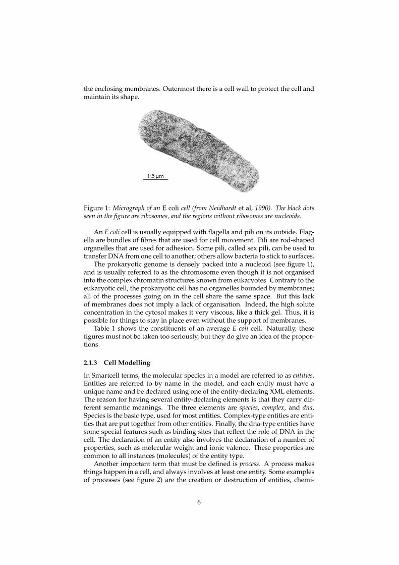
Escherichia coli (or E coli for short) is a gram-negative, rod-shaped bacteriumwhich is typically about 2 µm long and has a cross-section diameter of about1 µm (figure 1). The interior of the cell, the cytosol, is covered by a membranecalled the cell membrane or cytoplasmic membrane. This membrane is in turnsurrounded by another membrane called the outer membrane, a special fea-ture of gram-negative bacteria. The membranes restrict the passage of macro-molecules and some small molecules. The space between the cell membraneand the outer membrane is called the periplasmatic space. The solute compo-sition of the periplasmatic space is very different from that on either side of

5

the enclosing membranes. Outermost there is a cell wall to protect the cell andmaintain its shape.

Figure 1: Micrograph of an E coli cell (from Neidhardt et al, 1990). The black dotsseen in the figure are ribosomes, and the regions without ribosomes are nucleoids.

An E coli cell is usually equipped with flagella and pili on its outside. Flag-ella are bundles of fibres that are used for cell movement. Pili are rod-shapedorganelles that are used for adhesion. Some pili, called sex pili, can be used totransfer DNA from one cell to another; others allow bacteria to stick to surfaces.

The prokaryotic genome is densely packed into a nucleoid (see figure 1),and is usually referred to as the chromosome even though it is not organisedinto the complex chromatin structures known from eukaryotes. Contrary to theeukaryotic cell, the prokaryotic cell has no organelles bounded by membranes;all of the processes going on in the cell share the same space. But this lackof membranes does not imply a lack of organisation. Indeed, the high soluteconcentration in the cytosol makes it very viscous, like a thick gel. Thus, it ispossible for things to stay in place even without the support of membranes.

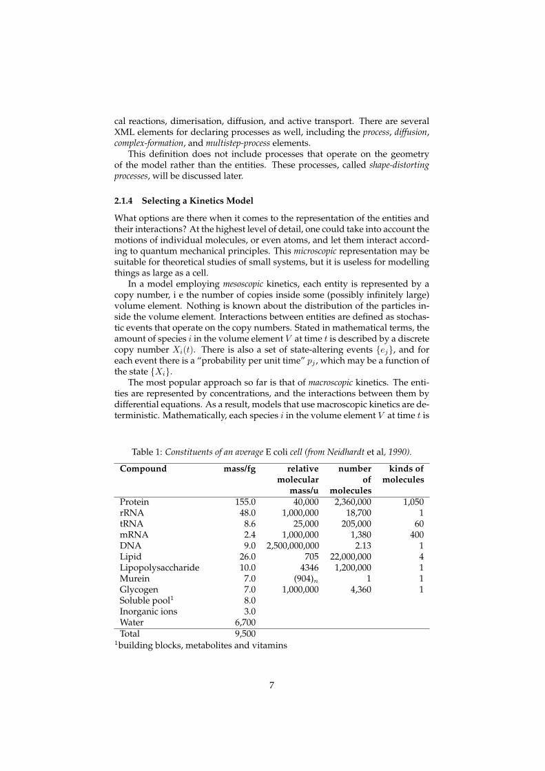
Table 1 shows the constituents of an average E coli cell. Naturally, thesefigures must not be taken too seriously, but they do give an idea of the propor-tions.

2.1.3 Cell Modelling

In Smartcell terms, the molecular species in a model are referred to as entities.Entities are referred to by name in the model, and each entity must have aunique name and be declared using one of the entity-declaring XML elements.The reason for having several entity-declaring elements is that they carry dif-ferent semantic meanings. The three elements are species, complex, and dna.Species is the basic type, used for most entities. Complex-type entities are enti-ties that are put together from other entities. Finally, the dna-type entities havesome special features such as binding sites that reflect the role of DNA in thecell. The declaration of an entity also involves the declaration of a number ofproperties, such as molecular weight and ionic valence. These properties arecommon to all instances (molecules) of the entity type.

Another important term that must be defined is process. A process makesthings happen in a cell, and always involves at least one entity. Some examplesof processes (see figure 2) are the creation or destruction of entities, chemi-

6

cal reactions, dimerisation, diffusion, and active transport. There are severalXML elements for declaring processes as well, including the process, diffusion,complex-formation, and multistep-process elements.

This definition does not include processes that operate on the geometryof the model rather than the entities. These processes, called shape-distortingprocesses, will be discussed later.

2.1.4 Selecting a Kinetics Model

What options are there when it comes to the representation of the entities andtheir interactions? At the highest level of detail, one could take into account themotions of individual molecules, or even atoms, and let them interact accord-ing to quantum mechanical principles. This microscopic representation may besuitable for theoretical studies of small systems, but it is useless for modellingthings as large as a cell.

In a model employing mesoscopic kinetics, each entity is represented by acopy number, i e the number of copies inside some (possibly infinitely large)volume element. Nothing is known about the distribution of the particles in-side the volume element. Interactions between entities are defined as stochas-tic events that operate on the copy numbers. Stated in mathematical terms, theamount of species i in the volume element V at time t is described by a discretecopy number Xi(t). There is also a set of state-altering events {ej}, and foreach event there is a “probability per unit time” pj , which may be a function ofthe state {Xi}.

The most popular approach so far is that of macroscopic kinetics. The enti-ties are represented by concentrations, and the interactions between them bydifferential equations. As a result, models that use macroscopic kinetics are de-terministic. Mathematically, each species i in the volume element V at time t is

Table 1: Constituents of an average E coli cell (from Neidhardt et al, 1990).

Compound mass/fg relativemolecular

mass/u

numberof

molecules

kinds ofmolecules

Protein 155.0 40,000 2,360,000 1,050rRNA 48.0 1,000,000 18,700 1tRNA 8.6 25,000 205,000 60mRNA 2.4 1,000,000 1,380 400DNA 9.0 2,500,000,000 2.13 1Lipid 26.0 705 22,000,000 4Lipopolysaccharide 10.0 4346 1,200,000 1Murein 7.0 (904)n 1 1Glycogen 7.0 1,000,000 4,360 1Soluble pool1 8.0Inorganic ions 3.0Water 6,700Total 9,500

1building blocks, metabolites and vitamins

7

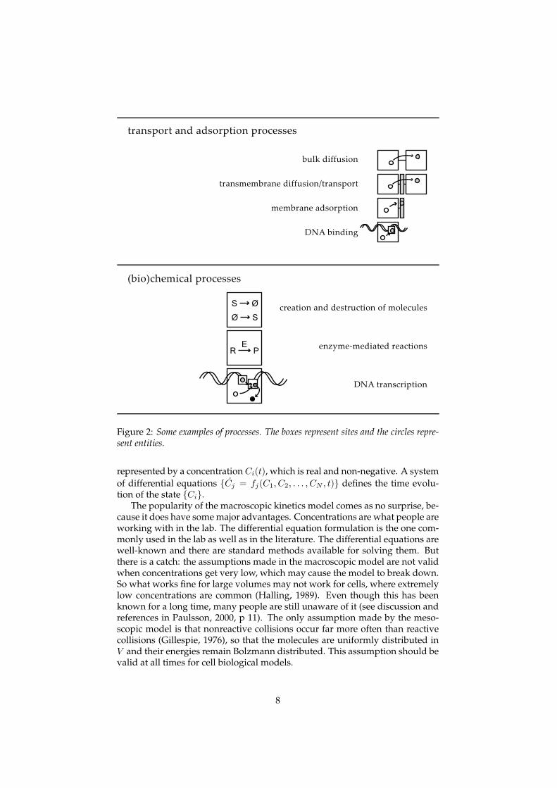
Figure 2: Some examples of processes. The boxes represent sites and the circles repre-sent entities.

represented by a concentration Ci(t), which is real and non-negative. A systemof differential equations {Cj = fj(C1, C2, . . . , CN , t)} defines the time evolu-tion of the state {Ci}.

The popularity of the macroscopic kinetics model comes as no surprise, be-cause it does have some major advantages. Concentrations are what people areworking with in the lab. The differential equation formulation is the one com-monly used in the lab as well as in the literature. The differential equations arewell-known and there are standard methods available for solving them. Butthere is a catch: the assumptions made in the macroscopic model are not validwhen concentrations get very low, which may cause the model to break down.So what works fine for large volumes may not work for cells, where extremelylow concentrations are common (Halling, 1989). Even though this has beenknown for a long time, many people are still unaware of it (see discussion andreferences in Paulsson, 2000, p 11). The only assumption made by the meso-scopic model is that nonreactive collisions occur far more often than reactivecollisions (Gillespie, 1976), so that the molecules are uniformly distributed inV and their energies remain Bolzmann distributed. This assumption should bevalid at all times for cell biological models.

8

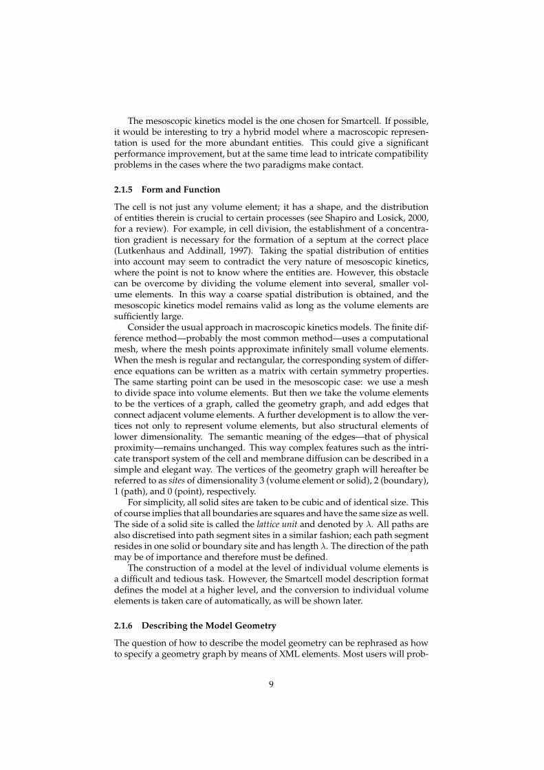
The mesoscopic kinetics model is the one chosen for Smartcell. If possible,it would be interesting to try a hybrid model where a macroscopic represen-tation is used for the more abundant entities. This could give a significantperformance improvement, but at the same time lead to intricate compatibilityproblems in the cases where the two paradigms make contact.

2.1.5 Form and Function

The cell is not just any volume element; it has a shape, and the distributionof entities therein is crucial to certain processes (see Shapiro and Losick, 2000,for a review). For example, in cell division, the establishment of a concentra-tion gradient is necessary for the formation of a septum at the correct place(Lutkenhaus and Addinall, 1997). Taking the spatial distribution of entitiesinto account may seem to contradict the very nature of mesoscopic kinetics,where the point is not to know where the entities are. However, this obstaclecan be overcome by dividing the volume element into several, smaller vol-ume elements. In this way a coarse spatial distribution is obtained, and themesoscopic kinetics model remains valid as long as the volume elements aresufficiently large.

Consider the usual approach in macroscopic kinetics models. The finite dif-ference method—probably the most common method—uses a computationalmesh, where the mesh points approximate infinitely small volume elements.When the mesh is regular and rectangular, the corresponding system of differ-ence equations can be written as a matrix with certain symmetry properties.The same starting point can be used in the mesoscopic case: we use a meshto divide space into volume elements. But then we take the volume elementsto be the vertices of a graph, called the geometry graph, and add edges thatconnect adjacent volume elements. A further development is to allow the ver-tices not only to represent volume elements, but also structural elements oflower dimensionality. The semantic meaning of the edges—that of physicalproximity—remains unchanged. This way complex features such as the intri-cate transport system of the cell and membrane diffusion can be described in asimple and elegant way. The vertices of the geometry graph will hereafter bereferred to as sites of dimensionality 3 (volume element or solid), 2 (boundary),1 (path), and 0 (point), respectively.

For simplicity, all solid sites are taken to be cubic and of identical size. Thisof course implies that all boundaries are squares and have the same size as well.The side of a solid site is called the lattice unit and denoted by λ. All paths arealso discretised into path segment sites in a similar fashion; each path segmentresides in one solid or boundary site and has length λ. The direction of the pathmay be of importance and therefore must be defined.

The construction of a model at the level of individual volume elements isa difficult and tedious task. However, the Smartcell model description formatdefines the model at a higher level, and the conversion to individual volumeelements is taken care of automatically, as will be shown later.

2.1.6 Describing the Model Geometry

The question of how to describe the model geometry can be rephrased as howto specify a geometry graph by means of XML elements. Most users will prob-

9

ably find that “rod-shaped” is a better description of the E Coli geometry thana detailed list of sites and connecting edges. On the other hand, some modelgeometries may be so specific that no high-level description (e g rod-shaped)will do.

The solution to this dilemma is to use a low-level description format, andsupply some pre-defined model geometry modules with the framework. Thisleaves us with the question of how to define an arbitrary geometry graph usingXML elements.

But first the important term region must be defined. When building a model,one frequently needs to refer to a set of sites collectively. This is accomplishedthrough the introduction of the region. Mathematically, the model geometryis represented by an undirected graph G = 〈S,E〉 where S is the set of sites(vertices) and E is the set of edges connecting the sites. A region R ⊆ S is a setof sites. Regions may be defined as part of the model geometry, and they canalso be constructed from existing regions by means of the set operations union(A ∪ B), intersection (A ∩ B), difference (A\B), and complement (Ac). Thereare also two special regions called empty (= ∅), and universe (= S). A regionwhere all sites have the same dimensionality (solid, boundary, path, or point)is called homogeneous.

In its current version, the Smartcell DTD does not contain any elements fordefining the geometry graph. However, one way of doing this that I call thelattice operation method will be presented here. Although not able to define re-ally arbitrary geometry graphs, it is able to describe most, if not all, physicallyrelevant geometry graphs.

The lattice operation method works much like a pixel-based paint pro-gramme. The method starts with the introduction of a lattice; a three-dimen-sional scaffold where volume elements (solid-type sites) can be attached. Atwo-dimensional model can be built by letting the lattice have unit thicknessin one dimension.

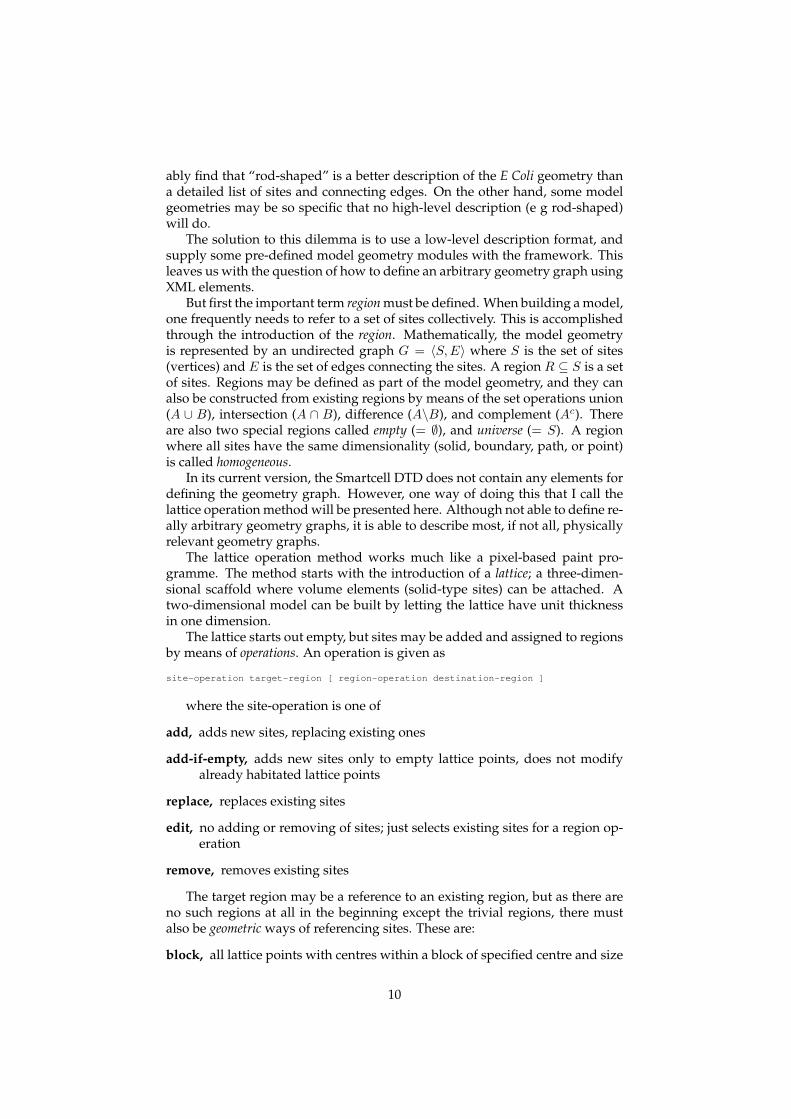
The lattice starts out empty, but sites may be added and assigned to regionsby means of operations. An operation is given as

site-operation target-region [ region-operation destination-region ]

where the site-operation is one of

add, adds new sites, replacing existing ones

add-if-empty, adds new sites only to empty lattice points, does not modifyalready habitated lattice points

replace, replaces existing sites

edit, no adding or removing of sites; just selects existing sites for a region op-eration

remove, removes existing sites

The target region may be a reference to an existing region, but as there areno such regions at all in the beginning except the trivial regions, there mustalso be geometric ways of referencing sites. These are:

block, all lattice points with centres within a block of specified centre and size

10

ellipsoid, all lattice points with centres within an ellipsoid of specified centreand size

border, a border, one lattice unit thick, around a specified region

The last part of the operation specifies an optional region operation to becarried out on the sites identified by the site operation and target region. Validregion operations are:

add-to-region, the sites are added to the destination region

remove-from-region, the sites are removed from the destination region

With the solid sites in place we can start adding other geometry features aswell. There are a number of operations available for this purpose:

interconnect, takes one region as parameter; connects all neighbour pairs forwhich both neighbours belong to the region.

boundary, takes three regions A, B, and C as parameters; adds boundary sitesbetween every region A-region B neighbour pair and assigns them toregion C.

path, takes a list of point coordinates and a name as parameters. The path isdiscretised to fit the lattice and broken into path segment sites, which areassigned to a region named after the path.

point, takes a name and a set of coordinates as parameters; adds a point site tothe geomery graph and assigns it to the region with the specified name.

It should be stressed that this is just one way of defining the model geome-try; there may be other alternatives better suited for the needs of the Smartcellframework. We shall finish this section with an example of how to describe asimple coliform model geometry with this notation:

lattice unit( .2 ) size( 2.2, 2.2, 2.2 )

An initialisation operation that was not described above. The lattice unit(the distance between two lattice points) is taken to be .2 µm, and the size ofthe lattice to be 2.2 µm in each spatial dimension. The lattice is centered at (0,0, 0).

add-if-empty ellipsoid( (0, 0, 0), (2, 1, 1) ) add-to-region "cytosol"

Create sites at the mesh points within an ellipsoid with centre at origo andlength 2 µm in the x direction and 1 µm in the y and z directions, then assignthe sites to the cytosol region

interconnect "cytosol"

Connect neighbour sites within the cytosol.

add-if-empty border( "cytosol" ) add-to-region "surroundings"

Create a border around the cytosol and name it “surroundings”.

interconnect "surroundings"

11

Connect neighbour sites within the surroundings. Note that some sur-roundings sites may still be unconnected due to the jagginess of the discretisedellipsoid’s edge.

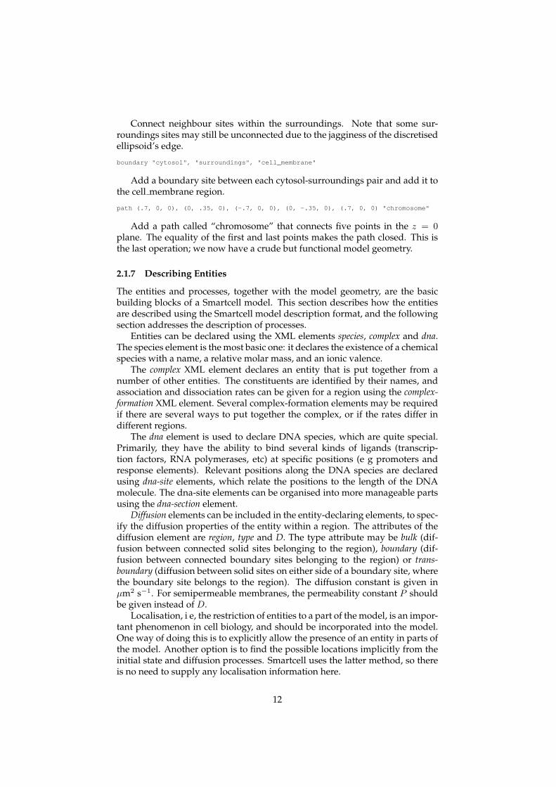
boundary "cytosol", "surroundings", "cell_membrane"

Add a boundary site between each cytosol-surroundings pair and add it tothe cell membrane region.

path (.7, 0, 0), (0, .35, 0), (-.7, 0, 0), (0, -.35, 0), (.7, 0, 0) "chromosome"

Add a path called “chromosome” that connects five points in the z = 0plane. The equality of the first and last points makes the path closed. This isthe last operation; we now have a crude but functional model geometry.

2.1.7 Describing Entities

The entities and processes, together with the model geometry, are the basicbuilding blocks of a Smartcell model. This section describes how the entitiesare described using the Smartcell model description format, and the followingsection addresses the description of processes.

Entities can be declared using the XML elements species, complex and dna.The species element is the most basic one: it declares the existence of a chemicalspecies with a name, a relative molar mass, and an ionic valence.

The complex XML element declares an entity that is put together from anumber of other entities. The constituents are identified by their names, andassociation and dissociation rates can be given for a region using the complex-formation XML element. Several complex-formation elements may be requiredif there are several ways to put together the complex, or if the rates differ indifferent regions.

The dna element is used to declare DNA species, which are quite special.Primarily, they have the ability to bind several kinds of ligands (transcrip-tion factors, RNA polymerases, etc) at specific positions (e g promoters andresponse elements). Relevant positions along the DNA species are declaredusing dna-site elements, which relate the positions to the length of the DNAmolecule. The dna-site elements can be organised into more manageable partsusing the dna-section element.

Diffusion elements can be included in the entity-declaring elements, to spec-ify the diffusion properties of the entity within a region. The attributes of thediffusion element are region, type and D. The type attribute may be bulk (dif-fusion between connected solid sites belonging to the region), boundary (dif-fusion between connected boundary sites belonging to the region) or trans-boundary (diffusion between solid sites on either side of a boundary site, wherethe boundary site belongs to the region). The diffusion constant is given inµm2 s−1. For semipermeable membranes, the permeability constant P shouldbe given instead of D.

Localisation, i e, the restriction of entities to a part of the model, is an impor-tant phenomenon in cell biology, and should be incorporated into the model.One way of doing this is to explicitly allow the presence of an entity in parts ofthe model. Another option is to find the possible locations implicitly from theinitial state and diffusion processes. Smartcell uses the latter method, so thereis no need to supply any localisation information here.

12

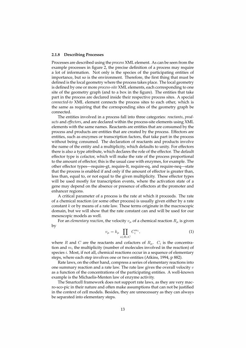
2.1.8 Describing Processes

Processes are described using the process XML element. As can be seen from theexample processes in figure 2, the precise definition of a process may requirea lot of information. Not only is the species of the participating entities ofimportance, but so is the environment. Therefore, the first thing that must bedefined is the local geometry where the process takes place. The local geometryis defined by one or more process-site XML elements, each corresponding to onesite of the geometry graph (and to a box in the figure). The entities that takepart in the process are declared inside their respective process sites. A specialconnected-to XML element connects the process sites to each other, which isthe same as requiring that the corresponding sites of the geometry graph beconnected.

The entities involved in a process fall into three categories: reactants, prod-ucts and effectors, and are declared within the process-site elements using XMLelements with the same names. Reactants are entities that are consumed by theprocess and products are entities that are created by the process. Effectors areentities, such as enzymes or transcription factors, that take part in the processwithout being consumed. The declaration of reactants and products involvethe name of the entity and a multiplicity, which defaults to unity. For effectorsthere is also a type attribute, which declares the role of the effector. The defaulteffector type is cofactor, which will make the rate of the process proportionalto the amount of effector; this is the usual case with enzymes, for example. Theother effector types—require-gt, require-lt, require-eq, and require-neq—statethat the process is enabled if and only if the amount of effector is greater than,less than, equal to, or not equal to the given multiplicity. These effector typeswill be used mostly for transcription events, where the activation state of agene may depend on the absence or presence of effectors at the promoter andenhancer regions.

A critical parameter of a process is the rate at which it proceeds. The rateof a chemical reaction (or some other process) is usually given either by a rateconstant k or by means of a rate law. These terms originate in the macroscopicdomain, but we will show that the rate constant can and will be used for ourmesoscopic models as well.

For an elementary reaction, the velocity vµ of a chemical reaction Rµ is givenby

vµ = kµ

∏

i∈R∪C

Cmii , (1)

where R and C are the reactants and cofactors of Rµ. Ci is the concentra-tion and mi the multiplicity (number of molecules involved in the reaction) ofspecies i. Most, if not all, chemical reactions occur in a sequence of elementarysteps, where each step involves one or two entities (Atkins, 1994, p 882).

Rate laws, on the other hand, compress a series of elementary reactions intoone summary reaction and a rate law. The rate law gives the overall velocity vas a function of the concentrations of the participating entities. A well-knownexample is the Michaelis-Menten law of enzyme activity.

The Smartcell framework does not support rate laws, as they are very mac-ro-sco-pic in their nature and often make assumptions that can not be justifiedin the context of cell models. Besides, they are unnecessary as they can alwaysbe separated into elementary steps.

13

The rate constant k of a process is declared using the rate attribute. If theprocess is reversible, the reverse rate can also be declared using the reverse-rate attribute (one must be very careful with effectors of the limiting kind inreversible reactions, as the reverse process is formed by changing all reactantsto products and vice versa. The effectors are left as they are, which may leadto unexpected behaviour from the limiting effectors). The rate is given as anumerical constant or an expression, and there is no way of attaching a unit toit in the model description file. Therefore, there may be no doubt about whichunit is used.

Let us consider the subject of units for a moment. The unit of preferencefor concentrations is the Molar (M), where 1 M = 1 mol per dm3. The concen-trations of solutes in a cell ranges from a few nanomoles (corresponding to asingle molecule) to tens of millimolars. Entities bound to a membrane (residingin a boundary site) can be quantified by a surface density, and entities bound toa fiber (in a path segment site) by a path density. For reasons of consistency, allconcentrations are given in mol per dmd, where d is the dimensionality (i e, thenumber of spatial dimensions). When there are several entities from differentsites involved in a process, the units tend to get quite complex. This should notoccur frequently, though.

A multistep process is a special kind of process, declared by the multistep-process XML element. It is an adaptation of a feature presented in the paper byGibson and Bruck (2000), that is likely to give an enormous performance im-provement for certain kinds of processes. The processes of interest are chainsof irreversible, monomolecular processes, such as transcription and transla-tion. Consider a chain of n reactions, each with the same reaction parameter c.Each reaction turns one reactant molecule Si into one product molecule Si+1,which is at the same time the reactant of the next reaction. If none of the inter-mediate products is of interest, the whole chain of processes can be reduced toone process, turning S0 directly into Sn. The multistep-process element is usedin the same way as the process element with the following exceptions: theremust be exactly one reactant entity and one product entity, there is an attributen that defines the number of steps in the process, and there is no reverse-rateattribute.

There is one class of processes yet to be described: the shape-distortingprocesses. These processes incorporate the mechanisms that affect the modelgeometry into the model itself. Cell growth, cell fission and DNA diffusion areexamples of such mechanisms. The question is how to specify such a process;it is out of scope for this work, but should be considered in the future.

One possibility is specify rules on the lattice level, like cellular automata,where the rules may involve entities in the affected sites. As I see it, this im-plicit formulation where the outcome is not necessarily known is the most in-teresting one, because it captures the underlying physics albeit in a simplifiedway. However, it will probably be quite difficult to define the rules.

Another alternative is to explicitly specify the changes to the geometry thathappen in a sequence, possibly with requirements that must be fulfilled beforethe next step can take place. This should not be too difficult to implement asa first step, and may give a very accurate description of e g cell growth andfission.

14

2.2 Simulation

Simulation is the process of performing experiments on a model. Using simu-lation techniques instead of actually performing the experiments can save timeand money; in addition there are experiments that are impossible to carry outin reality, that may be possible to simulate. The validity of the model is cru-cial; if the model is invalid, the simulation results will also be invalid. This issometimes referred to as the GIGO principle: garbage in yields garbage out.

A model that accurately describes a system can be used to test a hypothesisconcerning the system, using e g the well-known chi-square test. The anal-ogy with real experimental work continues into the data analysis domain: thenumber of trajectories (simulation runs) required to reach a certain level of con-fidence is of course equal to the number of real experiments it would take toreach the same confidence level.

Smartcell models are models of living cells. What kind of results can begained from simulations on such a model? When building a model, or tuningits parameters, one is frequently interested in the concentration or spatial dis-tribution of entities. To find them, one can set up a dummy experiment, wherethe cell is simply “living” under normal conditions, while the appropriate mea-surements are made. Other simulations that require a working model are themeasurement of the relaxation time following a perturbation, or to see how themodification of one model parameter affects other parts of the model.

2.2.1 Simulation Parameters

A real, wet experiment in cell biology is usually carried out as follows: a sys-tem is set up by growing cells under controlled conditions, then the system isdisturbed in some way, e g by moving the cells to a new growth medium. Ob-servations are made by taking samples from the cell culture and performingmeasurements on them. In some cases it may also be possible to perform themeasurements in vivo. Eventually, conclusions are drawn from the observa-tions. A Smartcell simulation run closely mimics this procedure, as it requiresthe definition of an initial state, an optional set of constraints and a set of obser-vations. These things are all defined by XML elements with the same names, aswill be described next.

The initial state describes “what is where and how much” at the start ofthe simulation run. The initial-state element defines the concentration of anentity in a homogeneous region. Several initial-state elements may be requiredif the concentration varies throughout the model. The concentration (in molper dm−d, where d is the dimensionality of the region) is given as a numericalexpression contained within the initial-state element, and may be a function ofspatial coordinates.

Constraints regulate the amount of a species after the start of the simulation.Constraints should be used with care, as they can lead to unphysical resultsif misused. But, when used in a sensible way, constraints can be a powerfultool. This is another advantage of simulation, as some constraints may be verydifficult or even impossible to enforce on the real system. Constraints are de-fined in the same way as initial states, but as functions of time. A time interval[tstart, tend) when the constraint is active can also be specified; if none is given,it defaults to [0,∞).

15

A special XML element is used for specifying how DNA entities are mappedto paths; it is called dna-mapping and takes an entity name and a path as at-tributes. One can consider this element as a special case of the constraint ele-ment.

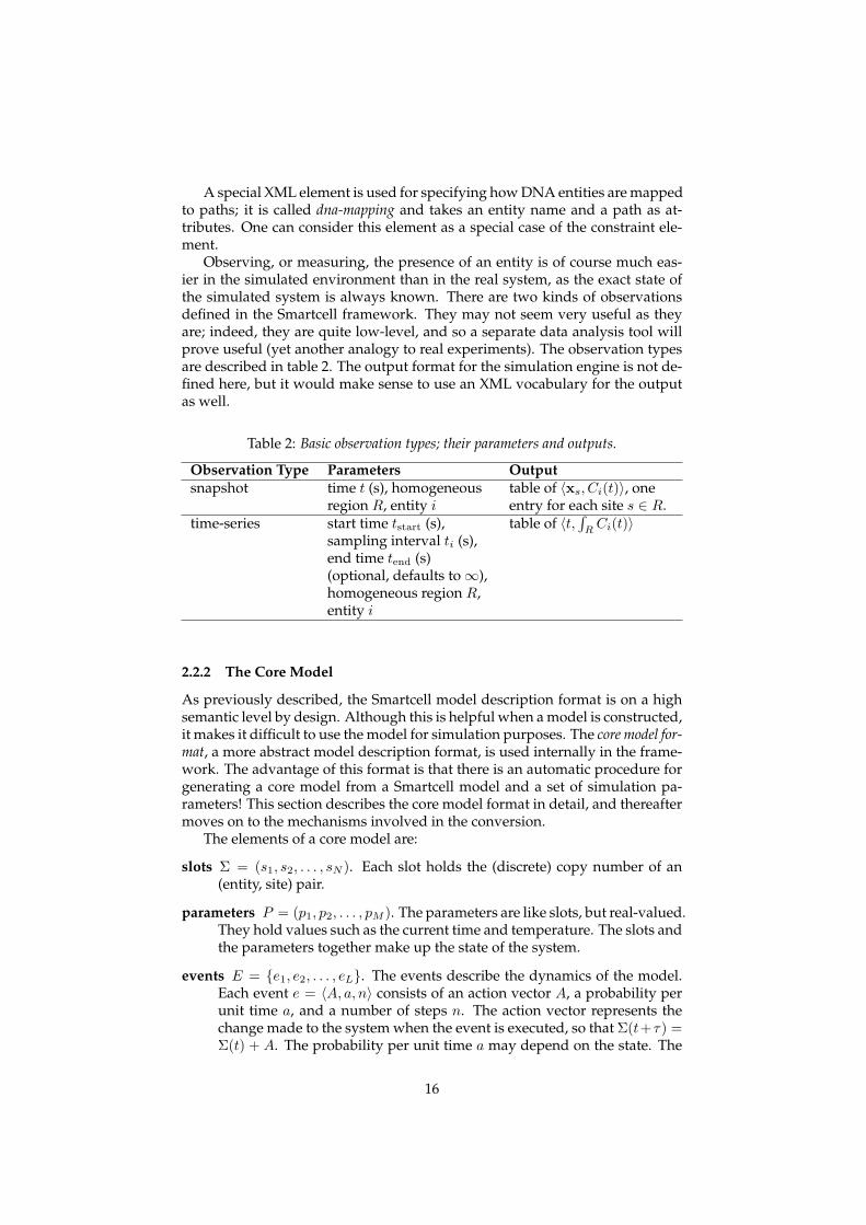
Observing, or measuring, the presence of an entity is of course much eas-ier in the simulated environment than in the real system, as the exact state ofthe simulated system is always known. There are two kinds of observationsdefined in the Smartcell framework. They may not seem very useful as theyare; indeed, they are quite low-level, and so a separate data analysis tool willprove useful (yet another analogy to real experiments). The observation typesare described in table 2. The output format for the simulation engine is not de-fined here, but it would make sense to use an XML vocabulary for the outputas well.

Table 2: Basic observation types; their parameters and outputs.

Observation Type Parameters Outputsnapshot time t (s), homogeneous

region R, entity itable of 〈xs, Ci(t)〉, oneentry for each site s ∈ R.

time-series start time tstart (s),sampling interval ti (s),end time tend (s)(optional, defaults to ∞),homogeneous region R,entity i

table of 〈t, ∫R

Ci(t)〉

2.2.2 The Core Model

As previously described, the Smartcell model description format is on a highsemantic level by design. Although this is helpful when a model is constructed,it makes it difficult to use the model for simulation purposes. The core model for-mat, a more abstract model description format, is used internally in the frame-work. The advantage of this format is that there is an automatic procedure forgenerating a core model from a Smartcell model and a set of simulation pa-rameters! This section describes the core model format in detail, and thereaftermoves on to the mechanisms involved in the conversion.

The elements of a core model are:

slots Σ = (s1, s2, . . . , sN ). Each slot holds the (discrete) copy number of an(entity, site) pair.

parameters P = (p1, p2, . . . , pM ). The parameters are like slots, but real-valued.They hold values such as the current time and temperature. The slots andthe parameters together make up the state of the system.

events E = {e1, e2, . . . , eL}. The events describe the dynamics of the model.Each event e = 〈A, a, n〉 consists of an action vector A, a probability perunit time a, and a number of steps n. The action vector represents thechange made to the system when the event is executed, so that Σ(t+τ) =Σ(t) + A. The probability per unit time a may depend on the state. The

16

number of steps is usually one. When n 6= 1, the event is carried out inn steps, each with probability a per unit time (compare to the multistepprocesses). In this case, a must be constant in order for the event to bephysically valid.

constraints C = {c1, c2, . . . , cK}, each constraint c = 〈n, α, T 〉 constraining slotn or parameter n−N (N is the number of slots) to the expression α duringthe time interval T = [tstart, tend).

Contrary to the Smartcell model, the core model also includes initial state andcontraint information.

The conversion from a Smartcell model (including a geometry graph) anda set of simulation parameters into a core model is done as follows. Please notethat this conversion is valid for a static model only, i e, a model without shape-distorting processes. A non-static model would require a regeneration of thecore model each time the geometry changes (which is a complex operation, butnot impossible).

A final note before we start with the details of the conversion process: it isimportant to keep references from the core model back into the source model.The evaluation of data must be done in the context of the source model ratherthan the core model; without these references it will not be possible to make ameaningful interpretation of the simulation results.

To start with, the DNA sites must be added to the geometry graph. Themapping of dna species onto paths are specified using dna-mapping elements;for each such element, the DNA sites of the DNA species are projected on thepath and added to the geometry graph as point sites. A special kind of site,called a DNA pseudosite, is also added and then connected to all point sites.

Entities of all types (species, complex, and dna) are enumerated, and so areall sites in the geometry graph. Now, a trivial slot mapping is to let each (entity,site) pair correspond to a slot. The trivial slot mapping produces a dense mapmatrix. However, in most cases, an entity will only be found in a small numberof sites, making the actual mapping matrix very sparse. A method must bedeveloped to find out which slots will actually be used (i e, possibly nonzero),and remove the rest from the model. A further optimisation is to also removethe slots that necessarily remain constant throughout the simulation run, andhandle them separately.

Parameter-type simulation parameters are added as one parameter and oneassociated constraint to the core model.

Diffusion specifications and complex formations are converted into normalprocesses in an obvious way, except for the rates of diffusion processes whichneed a bit more work. This conversion procedure is described in appendix B.Reversible processes are split into two irreversible processes, also in an obviousway. This leaves us with a number of processes and multistep-processes toconvert into events.

In general, one process corresponds to several events. Consider a processwhich involves several entities residing in different process sites. Each map-ping of the process sites onto the geometry graph that conforms to the connec-tivity of the process sites corresponds to a separate event. With this mappingestablished, the action vector can be compiled from the set of reactants andproducts. An algorithm for the mapping has been constructed and is given inappendix C.

17

The Smartcell model description format uses the rate attribute k to definethe rate of a process. The core model, on the other hand, uses a “reaction proba-bility per unit time” a for the same purpose. This is where the stochastic natureof the core model shows. Although conceptually similar, the two are very dif-ferent on one point: k is defined with respect to concentrations and is thereforeindependent of volume. The reaction probability is defined as a function ofdiscrete copy numbers, and therefore changes with volume (unless the processis unimolecular). As will be shown, the reaction probability can be deducedfrom the rate, but first the reaction probability must be defined.

In a stochastic model the deterministic concept of “reaction rate” is mean-ingless; its stochastic counterpart is the reaction parameter c, or “reaction prob-ability per unit time”. The formal definition, given by Gillespie (1976), is:

cµδt ≡ average probability, to first order in δt, that a particular com-bination of Rµ reactant molecules will react accordingly in the nexttime interval δt.

This definition of c gives an average probability per unit time for each partic-ular combination of reactant molecules R and cofactors C. By multiplying cwith the number of available combinations h, given by

h =∏

i∈R∪C

(Xi

mi

), (2)

we get the propensity per unit time a. Here, Xi is the copy number of entity i,and mi is the multiplicity of the same entity. The limiting effectors—i e, thoseeffectors that are not of the cofactor type—are also included in h as unit step orimpulse factors, assuming the value 1 when the requirement is fulfilled and 0otherwise.

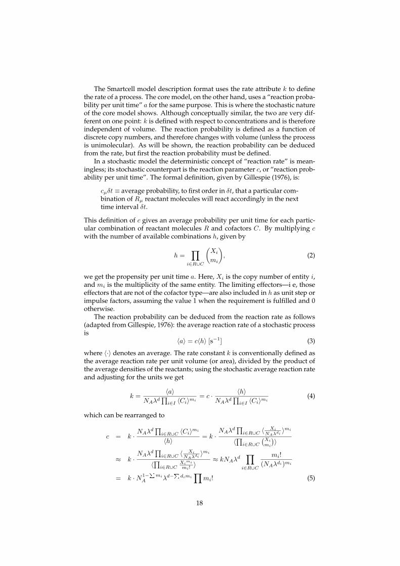
The reaction probability can be deduced from the reaction rate as follows(adapted from Gillespie, 1976): the average reaction rate of a stochastic processis

〈a〉 = c〈h〉 [s−1] (3)

where 〈·〉 denotes an average. The rate constant k is conventionally defined asthe average reaction rate per unit volume (or area), divided by the product ofthe average densities of the reactants; using the stochastic average reaction rateand adjusting for the units we get

k =〈a〉

NAλd∏

i∈I 〈Ci〉mi= c · 〈h〉

NAλd∏

i∈I 〈Ci〉mi(4)

which can be rearranged to

c = k · NAλd∏

i∈R∪C 〈Ci〉mi

〈h〉 = k ·NAλd

∏i∈R∪C 〈 Xi

NAλdi〉mi

〈∏i∈R∪C

(Xi

mi

)〉

≈ k ·NAλd

∏i∈R∪C 〈 Xi

NAλdi〉mi

〈∏i∈R∪CXi

mi

mi!〉 ≈ kNAλd

∏

i∈R∪C

mi!(NAλdi)mi

= k ·N1−Pmi

A λd−P dimi

∏mi! (5)

18

In this expression, λ is the lattice unit, NA is Avogadro’s number, and d is thedimensionality of the product sites (this must be identical for all products, orelse the rate is not well defined). di is the dimensionality of the site whereentity i resides.

2.2.3 Time Evolution of a Stochastic System

Now, with the core model in place, we can start making predictions. The timeevolution of the system can be found by setting up and solving the correspond-ing master equation. This is the same as a transformation of the core model intoa system of coupled differential equations in stochastic variables (see Gillespie,1976, for a summary of the master equation formalism). The solution of themaster equation contains all information there is about the system, but this ap-proach is typically impossible to use as the computing time required for thesolution explodes with increasing model size.

Fortunately, there are other methods. Whereas solving the master equationcan be seen as “finding all trajectories through state space at once”, it is alsopossible (and usually more computationally feasible) to find a number of tra-jectories, one at a time, and make an estimation. The method is simple: startfrom an initial state, then trace out the trajectory stepwise by choosing the nextstate according to calculated transition probabilities. The properties of the sys-tem can be estimated from a set of trajectories starting from the same initialstate. This method also has its drawbacks; one is the large number of trajec-tories that may be required for a good average estimation. There is also theprobability that some unusual states are never reached and therefore do notcontribute to the averages.

Stated in a formal way, the simulation algorithm in its most basic form is asfollows (Gillespie’s First Reaction Method, 1976, reformulated by Gibson andBruck, 2000):

1. initialise the state vector and set t ← 0

2. calculate the propensity function (probability per unit time) ai for eachevent i

3. for each event i, generate a putative time τi according to an exponentialdistribution with parameter ai

4. let µ be the event whose putative time τµ is least

5. update the slots to reflect the execution of event µ and let t ← t + τµ

6. go to step 2

Two things can be noted here: first, the algorithm does not handle multistepprocesses. Second, it draws the putative time from a negative exponential dis-tribution. We will continue by motivating the use of the negative exponentialdistribution and, at the same time, find a suitable distribution for multistepprocesses.

The transition from propensity per unit time a to putative execution timeτ is given by the following argument (from Lukkien et al, 1998): Assumingthat there is only a single enabled event—this is not a restriction as all events

19

are independent—with propensity a per unit time, and let τ be the time that itoccurs. By definition, the probability of the system staying in the initial statefor another interval δt is (1− aδt). Thus

P (τ ≥ t + δt) = P (τ ≥ t)(1− aδt). (6)

Rewriting and taking the limit δt → 0 gives

dP (τ ≥ t)δt

= −aP (τ ≥ t). (7)

Integration yieldsP (τ ≥ t) = exp(−at). (8)

Thus it can be seen that the putative time of execution τ has a negative expo-nential distribution with parameter a. Furthermore, this result can be gener-alised for multistep processes. It follows immediately from the definition ofthe gamma distribution that the putative time of execution for a multistep pro-cess with n steps is distributed as Γ(n, a). When n is one, this reduces to anegative exponential distribution. We therefore replace step 3 with “for eachevent i, generate a putative time τi according to Γ(n, a)”.

Gibson and Bruck (2000) also introduce a number of optimisations to the al-gorithm, resulting in what they call the “Next Reaction Method”. These modi-fications are:

• recalculate ai only when necessary. This can be accomplished as follows:maintain for each slot a list of dependent events, i e, those events whosepropensities depend on the slot. When the slot is modified, all events inits list are marked as “dirty” and will have their propensities recalculatedbefore the next event is selected.

• introduce absolute time—set τ ← t + τ in step 3, and t ← τ in step 5.Then store the τis as well, not just the ais. Thanks to absolute time, theseentities need only be recalculated when ai changes or when the event isexecuted.

• use an indexed priority queue for storing the τis. This guarantees thatthe updating of the queue will be efficient.

Gibson and Bruck also describe a way of reusing random numbers. They showthat, under certain circumstances, the putative execution times can be updatedby means of a scaling procedure instead of by another random number gen-eration. This does not seem to be a good idea to me, though. The scalingprocedure can be costly in itself, and there is also the danger of large round-offerrors.

The multistep event concept also comes from the same article. To handlemultistep events, we must add to the algorithm a priority queue Qi for eachmultistep event i, where the putative times of the events that are on their wayare stored. When the reactant slot is increased, a new putative time is gener-ated (as mentioned above) and put into the queue, and when the reactant slotdecreases (possibly, but not necessarily, due to the execution of the event), thefirst element of the queue—i e, the element with smallest τ—is removed fromthe queue.

20

The stochastic simulation concept requires a source of good random num-bers. This means that if a generator of pseudorandom numbers is used, asis customary on digital computers, it must have high randomness (no obvi-ous bias) and long period (all pseudorandom number generators have finiteperiods, i e, the sequence starts repeating sooner or later). A good choice forSmartcell is a pseudorandom number generator called Mersenne Twister (Mat-sumoto and Nishimura, 1998) that has a period of 219937 − 1. It is also fast—another critical property.

21

3 Results

This report describes the planning and construction of the Smartcell modellingand simulation framework. The framework is unique due to its combination oflocalisation and diffusion phenomena with mesoscopic kinetics. It also incor-porates most mechanisms of cell function in an elegant and consequent way.Not only the biological part, i e, the features of the cell, have been consideredduring the design of the framework, but also the physical and computationalaspects of modelling and simulation. The result is a flexible framework with awell-designed model description format and a simulation algorithm with highexpected performance.

The Smartcell project was initiated by Luis Serrano, who had been out-lining a simulation tool that would be helpful in genetic engineering. Withthis tool, it should be possible to perform simulation experiments on a modelof a cell, to see what would happen if the expression of a gene were up- ordown-regulated. The cell model should be assembled from modules, prefer-ably downloaded from public databases. Such a tool would of course not onlybe of use in the field of genetic engineering, but would be helpful in severalresearch areas.

The construction of a framework of this complexity simply cannot be ac-complished by one person in six months’ time. Instead, this work is to beseen as the initial phase of a larger project. The first step was to write downthe ideas, trying to break down the project into parts, and finding one or afew parts that could be implemented and tested separately. This was not soeasy, as it turned out—the parts were simply too intertwined. Instead, the goalwas set as the formulation of a theoretical foundation for the framework; themodel description format, the intermediate format and automatic conversionmethod, and the simulation algorithm. The initial time plan was revised to in-clude more theory and less programming. Many problems have been solved,others have been stated explicitly and formally, and yet others still remain tofind and solve. But these are left as an exercise to the reader.

The near future directions of the project, as I see it, are as follows:

implementation. A simple implementation of the described algorithms shouldnot be too difficult to achieve. Only when this exists will we know howthe algorithms perform.

modelling concepts. There are particularly two modelling concepts that needmore attention: the geometry description and the shape-distorting pro-cesses.

optimisations. Thanks to its modular organisation, the basis of the frameworkis a good target for optimisations. For example, it should be possible tomodify the simulation algorithm for parallel execution in a multicom-puter cluster. In general it will not be possible to partition the core modelinto independent parts, but an “optimist” parallelisation might performwell, provided the dependency between parts is small.

extensions. A model editor with a graphical user interface will probably beof great use for the model builders. An automatic database import toolwould also be useful, for importing e g DNA species from the genomedatabases or enzyme kinetics parameters from enzyme databases.

22

model construction and validation. This is the most important part: the who-le-cell simulation concept must be tested in itself! Is it at all possible tocreate an in silico cell? What is the typical execution time and accuracy ofa simulation run? This we cannot know until a model has been writtenand the simulation engine is up and running.

Acknowledgements

Many thanks to Luis Serrano (EMBL) for making the project possible, JohanElvnert (TTA) for financing the project, Erik Zeitler and Emmanuel Lacroix(EMBL) for discussions, Maria Ander (UTH/EMBL) for endless questions, MatsGustafsson (Signals and Systems Group, Uppsala University) for being the for-mal examiner, and Matti Nikkola (Department of Biology Education, UppsalaUniversity) for coordinating the diploma work.

23

4 ReferencesAtkins P W (1994). Physical Chemistry, 5th ed. Oxford University Press, OxfordGarfinkel D (1981). Computer modeling of metabolic pathways. TiBS 6:69–71Gibson M A and Bruck J (2000). Efficient Exact Stochastic Simulation of Chemical Sys-

tems with Many Species and Many Channels. J Phys Chem 104:1876–1889Gillespie D T (1976). A General Method for Numerically Simulating the Stochastic Time

Evolution of Coupled Chemical Reactions. J Comput Phys 22:403–434Halling P J (1989). Do the laws of chemistry apply to living cells? TiBS 14:317–318Heinrich R, Rapoport S M and Rapoport T A (1977). Metabolic Regulation and Mathe-

matical Models. Prog Biophys Molec Biol 32:1–82Lakshminarayanaiah N (1984). Equations of Membrane Biophysics. Academic Press, Inc.Lukkien J J, Segers J P L, Hilbers P A J, Gelten R J and Jansen A P J (1998). Efficient

Monte Carlo methods for the simulation of catalytic surface reactions.Phys Rev E 53:2598–2610

Lutkenhaus J and Addinall S G (1997). Bacterial Cell Division and the Z Ring. Annu RevBiochem 66:93–116

Matsumoto M and Nishimura T (1998). Mersenne Twister: A 623-dimensionally equidis-truibuted uniform pseudorandom number generator. ACM TOMACS 8:3–30

McAdams H H and Arkin A (1998). Simulation of prokaryotic genetic circuits. AnnuRev Biophys Biomol Struct 27:199–224

McAdams H H and Shapiro L (1995). Circuit Simulation of Genetic Networks.Science 269:650–656

Mendes P (1997). Biochemistry by numbers: simulation of biochemical pathways withGepasi 3. TiBS 22:361–363

Morton-Firth C J (1998). Stochastic simulation of cell signalling pathways. Ph D thesis,Cambridge

Neidhardt F C, Ingraham J L and Schaechter M (1990). Physiology of the Bacterial Cell,A Molecular Approach. Sinacor Associates, Inc. Sunderland, Massachusetts, USA

Paulsson J (2000). The Stochastic Nature of Intracellular Control Circuits. Ph D thesis,Uppsala

Schaff J and Loew L M (1999). The Virtual Cell. Pacific Symposium on Biocomputing4:228–239

Schaff J, Fink C C, Slepchenko B, Carson J H and Loew L M (1997). A General Compu-tational Framework for Modeling Cellular Structure and Function.Biophys J 73:1135–1146

Shapiro L and Losick R (2000). Dynamic Spatial Regulation in the Bacterial Cell.Cell 100:89–98

Smolen P, Baxter D A and Byrne J H (2000). Modeling Transcriptional Control in GeneNetworks—Methods, Recent Results, and Future Directions. Bull Math Biol 62:247–292

Stoffers H J, Sonnhammer E L L, Blommestijn G J F, Raat N J H and Westerhoff H V(1992). METASIM: object-oriented modelling of cell regulation. CABIOS 8:443–449

Stryer L (1995). Biochemistry, 4th ed. W H Freeman and Company, New YorkStundzia A B and Lumsden C J (1996). Stochastic Simulation of Coupled Reaction-

Diffusion Processes. J Comput Phys 127:196–207Tomita M, Hashimoto K, Takahashi K, Shimizu T S, Matsuzaki Y, Miyoshi F, Saito K,

Tanida S, Yugi K, Venter J C and Hutchison C A (1999). E-CELL: software environ-ment for whole-cell simulation. Bioinformatics 15:72–84

Uetz P, Giot L, Cagney G, Mansfield T A, Judson R S, Knight J R, Lockshon D, Narayan V,Srinivasan M, Pochart P, Qureshi-Emili A, Li Y, Godwin B, Conover D, Kalbfleisch T,Vijayadamodar G, Yang M, Johnston M, Fields S and Rothberg J M (2000). A compre-hensive analysis of protein/protein interactions in Sacccharomyces cerevisiae.Nature 403:623–627

24

A Model Description Format Reference

A Smartcell model consists of one or more module files. A module file is anXML document that conforms to the Smartcell DTD.

An XML file is a text document where the text is structured into elements.The elements carry a semantic meaning, which may differ between differentkinds of documents. The element boundaries are identified by tags; a sequenceof characters delimited by angle brackets. The similarity with HTML is not justin the name (Extensible Markup Language vs HyperText Markup Language);the documents also tend to look similar even though XML documents maydescribe things that have little or nothing in common with world wide webpages.

XML is far more strict than HTML when it comes to formal requirements.For a text file to be a valid XML document, there is an overall structure thatmust be followed, and the naming and nesting of tags is strictly regulated.It is also possible to reference a DTD (Document Type Definition) from thedocument, thereby adding an additional set of requirements on the attributes,order, and nesting of elements. Below is the DTD used for Smartcell modulefiles. Each element type is provided with a description and an example.

A.1 The Smartcell DTD



<!ELEMENT module ANY><!ATTLIST module

name CDATA #REQUIRED>



25

<!ELEMENT description ANY>

<!ELEMENT reference (authors, title, publication*)><!ELEMENT authors (#PCDATA)><!ELEMENT title (#PCDATA)><!ELEMENT publication (#PCDATA)>

<!ELEMENT date (#PCDATA)>

<!ELEMENT dbxref (xref_db, xref_db_id?)><!ELEMENT xref_db (#PCDATA)><!ELEMENT xref_db_id (#PCDATA)>



<!-- speciesThe most basic kind of entity: a chemical species.

Attributes:* ionic_valence: the charge of the particle; unit: electron charges* M: relative molecular mass; unit: u (the unified atomic mass unit)

26

The diffusivity of the entity may be specified by including diffusion elements.

Examples:<species name="ATP" /><species name="Cl-" ionic_valence="-1" M="35.45" />

--><!ELEMENT species (description?, diffusion*)><!ATTLIST species

name CDATA #REQUIREDionic_valence CDATA #IMPLIEDM CDATA #IMPLIED

>

<!ELEMENT complex (

description?,(diffusion|complex-formation)*

)><!ATTLIST complex

name CDATA #REQUIREDionic_valence CDATA #IMPLIEDM CDATA #IMPLIED

>

<!ELEMENT complex-formation (description?,complex-component,complex-component+

)><!ATTLIST complex-formation

region CDATA #REQUIREDtype (region|boundary|path|point) #REQUIREDrate CDATA #REQUIREDreverse-rate CDATA "0"

>

<!ELEMENT complex-component (description?)><!ATTLIST complex-component

name CDATA #REQUIREDmultiplicity CDATA "1"

>

<!-- dna

27

A DNA species.

The presence of relevant regions (such as genes, operators, promoters, etc)along the DNA molecule is marked out using dna-site elements. The dna-siteelements may be organised using dna-section elements. The dna-sections areinformational only and carry no information in themselves.

The diffusivity of a dna entity may be specified by including diffusionelements, but they will be ignored if the entity is mapped to a path.

Attributes:* name: the name of the DNA species or dna-site* size: the size of the DNA species; unit: base pairs* shape: shape of the DNA species; circular or linear* start, end: the position of the dna-site along the molecule; unit: base pairs* strand: the strand (sense or antisense)

Example:<dna name="chromosome" size="82727" shape="circular">

<dna-section><dna-site name="PDHC:E1b" start="426" end="916" />

</dna-section></dna>

--><!ELEMENT dna (description?, (dna-section|dna-site)*, diffusion*)><!ATTLIST dna

name CDATA #REQUIREDsize CDATA #REQUIREDshape (circular|linear) #REQUIRED

>

<!ELEMENT dna-section (description?, (dna-section|dna-site)*)>

<!ELEMENT dna-site (description?)><!ATTLIST dna-site

name CDATA #REQUIREDstart CDATA #REQUIREDend CDATA #IMPLIEDstrand (sense|antisense) "sense"

>

<!ELEMENT diffusion (description?)><!ATTLIST diffusion

region CDATA #REQUIREDtype (bulk|boundary|path|transboundary) #REQUIREDD CDATA #REQUIRED

>



28

<!ELEMENT process (description?, process-site+)><!ATTLIST process

name CDATA #REQUIREDrate CDATA #REQUIREDreverse-rate CDATA #IMPLIED

>

<!ELEMENT process-site ((reactant|effector|product)*, connected-to*)><!ATTLIST process-site

name CDATA #REQUIREDregion CDATA #REQUIREDtype (solid|boundary|path|point) #REQUIRED

>

<!ELEMENT connected-to EMPTY><!ATTLIST connected-to

name CDATA #REQUIREDdirection (positive|negative) #IMPLIED

>

<!ELEMENT reactant EMPTY><!ATTLIST reactant

name CDATA #REQUIREDmultiplicity CDATA "1"

>

<!ELEMENT effector EMPTY><!ATTLIST effector

name CDATA #REQUIREDtype (cofactor|require-gt|require-lt|require-eq|require-neq) "cofactor"multiplicity CDATA "1"

>

<!ELEMENT product EMPTY>

29

<!ATTLIST productname CDATA #REQUIREDmultiplicity CDATA "1"

>

<!ELEMENT multistep-process (description?, process-site+)><!ATTLIST multistep-process

name CDATA #REQUIREDrate CDATA #REQUIREDsteps CDATA #REQUIRED

>



<!ELEMENT initial-amount (#PCDATA|description)*><!ATTLIST initial-amount

entity CDATA #REQUIRED

30

region CDATA #REQUIREDtype (solid|boundary|path|point) #REQUIRED

>

<!ELEMENT dna-mapping EMPTY><!ATTLIST dna-mapping

entity CDATA #REQUIREDpath CDATA #REQUIRED

>

<!ELEMENT constraint (#PCDATA|description)*><!ATTLIST constraint

entity CDATA #REQUIREDregion CDATA #REQUIREDtype (solid|boundary|path|point) #REQUIREDstart-time CDATA "0"end-time CDATA #IMPLIED

>

<!-- parameterThis element is used to specify the value of a parameter.

Attributes:* name: the name of the parameter* start-time, end-time: the time interval where the parameter is defined,

defaults to [0, infinity). Unit: s

The element contains an expression that specifies the value of the parameter asa function of time.

The time intervals of two specifications of the same parameter may not overlap.

Example:

31

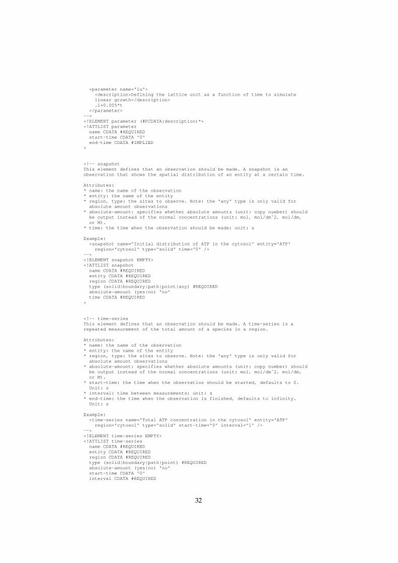
<parameter name="lu"><description>Defining the lattice unit as a function of time to simulatelinear growth</description>.1+0.005*t

</parameter>--><!ELEMENT parameter (#PCDATA|description)*><!ATTLIST parameter

name CDATA #REQUIREDstart-time CDATA "0"end-time CDATA #IMPLIED

>

<!ELEMENT snapshot EMPTY><!ATTLIST snapshot

name CDATA #REQUIREDentity CDATA #REQUIREDregion CDATA #REQUIREDtype (solid|boundary|path|point|any) #REQUIREDabsolute-amount (yes|no) "no"time CDATA #REQUIRED

>

<!ELEMENT time-series EMPTY><!ATTLIST time-series

name CDATA #REQUIREDentity CDATA #REQUIREDregion CDATA #REQUIREDtype (solid|boundary|path|point) #REQUIREDabsolute-amount (yes|no) "no"start-time CDATA "0"interval CDATA #REQUIRED

32

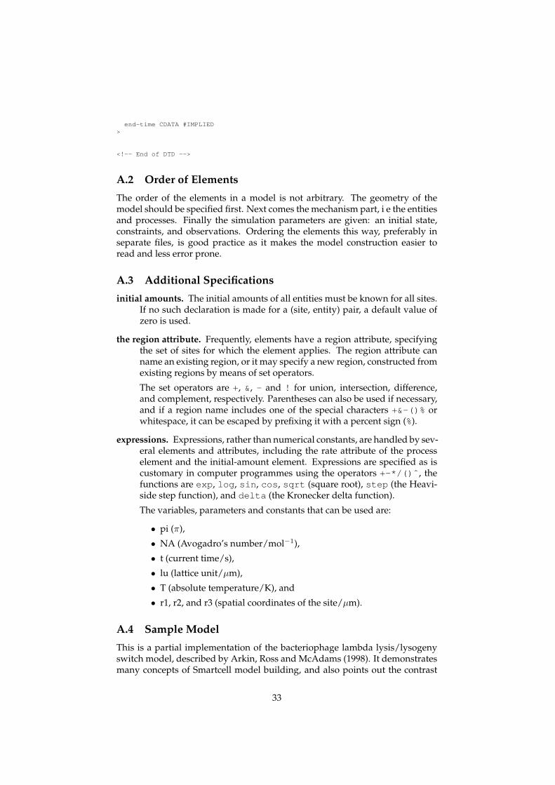
end-time CDATA #IMPLIED>



A.2 Order of Elements

The order of the elements in a model is not arbitrary. The geometry of themodel should be specified first. Next comes the mechanism part, i e the entitiesand processes. Finally the simulation parameters are given: an initial state,constraints, and observations. Ordering the elements this way, preferably inseparate files, is good practice as it makes the model construction easier toread and less error prone.

A.3 Additional Specifications

initial amounts. The initial amounts of all entities must be known for all sites.If no such declaration is made for a (site, entity) pair, a default value ofzero is used.

the region attribute. Frequently, elements have a region attribute, specifyingthe set of sites for which the element applies. The region attribute canname an existing region, or it may specify a new region, constructed fromexisting regions by means of set operators.

The set operators are +, &, - and ! for union, intersection, difference,and complement, respectively. Parentheses can also be used if necessary,and if a region name includes one of the special characters +&-()% orwhitespace, it can be escaped by prefixing it with a percent sign (%).

expressions. Expressions, rather than numerical constants, are handled by sev-eral elements and attributes, including the rate attribute of the processelement and the initial-amount element. Expressions are specified as iscustomary in computer programmes using the operators +-*/()ˆ , thefunctions are exp , log , sin , cos , sqrt (square root), step (the Heavi-side step function), and delta (the Kronecker delta function).

The variables, parameters and constants that can be used are:

• pi (π),

• NA (Avogadro’s number/mol−1),

• t (current time/s),

• lu (lattice unit/µm),

• T (absolute temperature/K), and

• r1, r2, and r3 (spatial coordinates of the site/µm).

A.4 Sample Model

This is a partial implementation of the bacteriophage lambda lysis/lysogenyswitch model, described by Arkin, Ross and McAdams (1998). It demonstratesmany concepts of Smartcell model building, and also points out the contrast

33

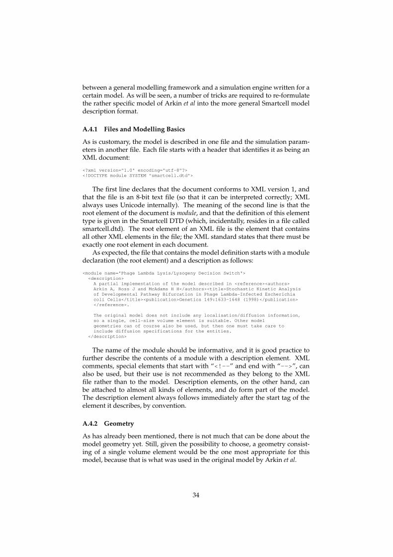
between a general modelling framework and a simulation engine written for acertain model. As will be seen, a number of tricks are required to re-formulatethe rather specific model of Arkin et al into the more general Smartcell modeldescription format.

A.4.1 Files and Modelling Basics

As is customary, the model is described in one file and the simulation param-eters in another file. Each file starts with a header that identifies it as being anXML document:

<?xml version="1.0" encoding="utf-8"?><!DOCTYPE module SYSTEM "smartcell.dtd">

The first line declares that the document conforms to XML version 1, andthat the file is an 8-bit text file (so that it can be interpreted correctly; XMLalways uses Unicode internally). The meaning of the second line is that theroot element of the document is module, and that the definition of this elementtype is given in the Smartcell DTD (which, incidentally, resides in a file calledsmartcell.dtd). The root element of an XML file is the element that containsall other XML elements in the file; the XML standard states that there must beexactly one root element in each document.

As expected, the file that contains the model definition starts with a moduledeclaration (the root element) and a description as follows:

<module name="Phage Lambda Lysis/Lysogeny Decision Switch"><description>

A partial implementation of the model described in <reference><authors>Arkin A, Ross J and McAdams H H</authors><title>Stochastic Kinetic Analysisof Developmental Pathway Bifurcation in Phage Lambda-Infected Escherichiacoli Cells</title><publication>Genetics 149:1633-1648 (1998)</publication></reference>.

The original model does not include any localisation/diffusion information,so a single, cell-size volume element is suitable. Other modelgeometries can of course also be used, but then one must take care toinclude diffusion specifications for the entities.

</description>

The name of the module should be informative, and it is good practice tofurther describe the contents of a module with a description element. XMLcomments, special elements that start with “ ”, canalso be used, but their use is not recommended as they belong to the XMLfile rather than to the model. Description elements, on the other hand, canbe attached to almost all kinds of elements, and do form part of the model.The description element always follows immediately after the start tag of theelement it describes, by convention.

A.4.2 Geometry

As has already been mentioned, there is not much that can be done about themodel geometry yet. Still, given the possibility to choose, a geometry consist-ing of a single volume element would be the one most appropriate for thismodel, because that is what was used in the original model by Arkin et al.

34

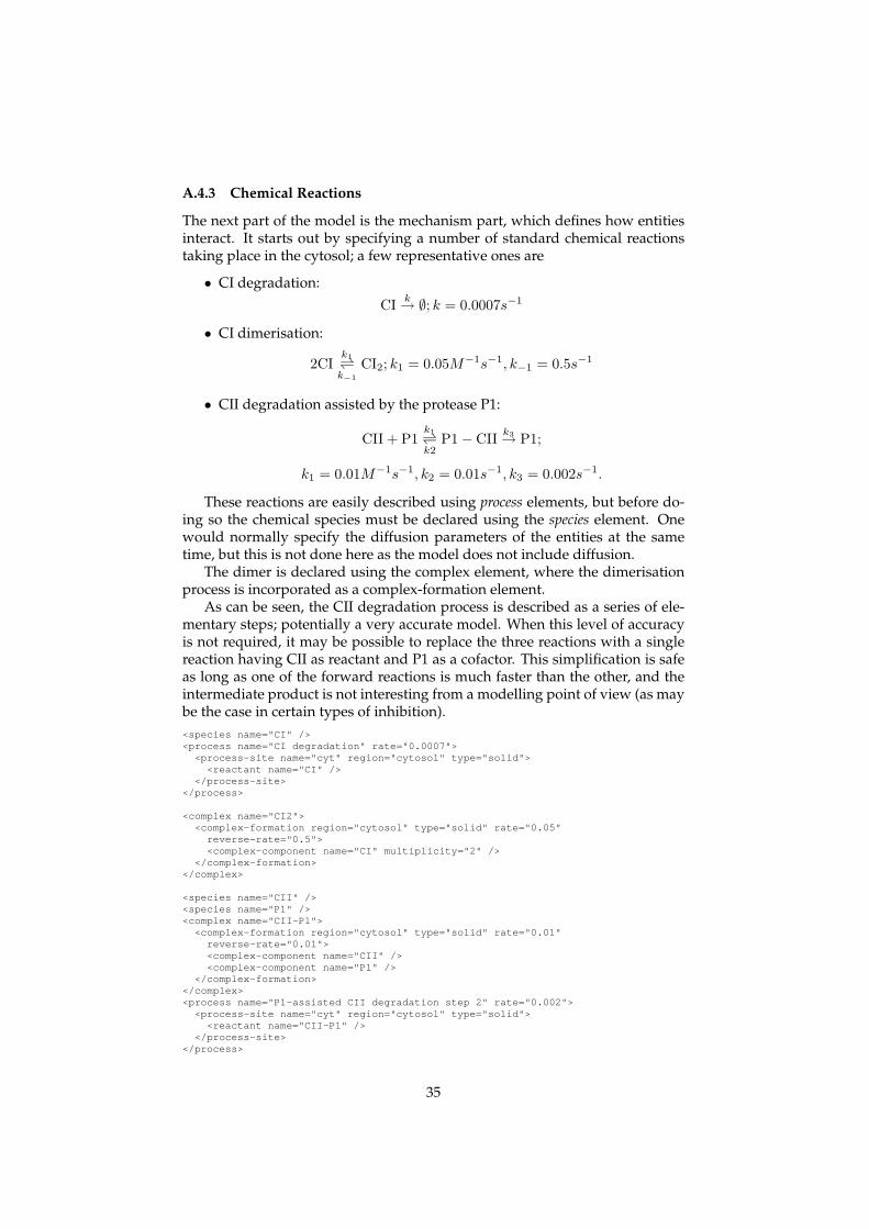
A.4.3 Chemical Reactions

The next part of the model is the mechanism part, which defines how entitiesinteract. It starts out by specifying a number of standard chemical reactionstaking place in the cytosol; a few representative ones are

• CI degradation:

CI k→ ∅; k = 0.0007s−1

• CI dimerisation:

2CIk1⇀↽

k−1

CI2; k1 = 0.05M−1s−1, k−1 = 0.5s−1

• CII degradation assisted by the protease P1:

CII + P1k1⇀↽k2

P1− CII k3→ P1;

k1 = 0.01M−1s−1, k2 = 0.01s−1, k3 = 0.002s−1.

These reactions are easily described using process elements, but before do-ing so the chemical species must be declared using the species element. Onewould normally specify the diffusion parameters of the entities at the sametime, but this is not done here as the model does not include diffusion.

The dimer is declared using the complex element, where the dimerisationprocess is incorporated as a complex-formation element.

As can be seen, the CII degradation process is described as a series of ele-mentary steps; potentially a very accurate model. When this level of accuracyis not required, it may be possible to replace the three reactions with a singlereaction having CII as reactant and P1 as a cofactor. This simplification is safeas long as one of the forward reactions is much faster than the other, and theintermediate product is not interesting from a modelling point of view (as maybe the case in certain types of inhibition).<species name="CI" /><process name="CI degradation" rate="0.0007">

<process-site name="cyt" region="cytosol" type="solid"><reactant name="CI" />


<complex name="CI2"><complex-formation region="cytosol" type="solid" rate="0.05"

reverse-rate="0.5"><complex-component name="CI" multiplicity="2" />

</complex-formation></complex>

<species name="CII" /><species name="P1" /><complex name="CII-P1">

<complex-formation region="cytosol" type="solid" rate="0.01"reverse-rate="0.01"><complex-component name="CII" /><complex-component name="P1" />

</complex-formation></complex><process name="P1-assisted CII degradation step 2" rate="0.002">

<process-site name="cyt" region="cytosol" type="solid"><reactant name="CII-P1" />


35

A.4.4 Transcription

A large part of the model is concerned with the transcription machinery andits regulation. The transcription part is therefore declared in a sub-module tomake the model description file easier to read:

<module name="Transcription">

Ignoring the DNA of the host cell—and most of the phage DNA as well—we can describe the interesting part of the phage DNA as follows:

<dna name="phage lambda genome" size="48502" shape="circular"><description>The interesting part of phage DNA (see figure 1 in the paper by

Arkin et al). Positional data taken from the database entry EMBL:LAMCG.The mRNA feature table entries are used for promoter and terminatorpositions, and misc_signal entries for the operator sites.

</description><dna-section>

<dna-site name="TL2" start="33100" strand="antisense" /><dna-site name="cIII" start="33299" end="33463" strand="antisense" /><dna-site name="TL1" start="33494" strand="antisense" /><dna-site name="TL1.end" start="33494" strand="antisense" /><dna-site name="n" start="35037" end="35438" strand="antisense" /><dna-site name="NutL" start="35518" end="35534" strand="antisense" /><dna-site name="OL1" start="35591" end="35607" strand="antisense" /><dna-site name="OL2" start="35615" end="35631" strand="antisense" /><dna-site name="PL" start="35582" strand="antisense" /><dna-site name="cI" start="37227" end="37940" strand="antisense" /><dna-site name="PRM" start="37940" strand="antisense" /><dna-site name="OR3" start="37951" end="37967" strand="sense" /><dna-site name="OR2" start="37974" end="37990" strand="sense" /><dna-site name="OR1" start="37998" end="38014" strand="sense" /><dna-site name="PR" start="38023" strand="sense" /><dna-site name="cro" start="38041" end="38241" strand="sense" /><dna-site name="NutR" start="38265" end="38281" strand="sense" /><dna-site name="PRE" start="38343" strand="antisense" /><dna-site name="OE1" start="38372" strand="antisense" /><dna-site name="OE2" start="38373" strand="antisense" /><dna-site name="TR1" start="38370" strand="sense" /><dna-site name="cII" start="38360" end="38653" strand="sense" /><dna-site name="o" start="38686" end="39585" strand="sense" /><dna-site name="p" start="39582" end="40283" strand="sense" /><dna-site name="TR2" start="40624" strand="sense" />

</dna-section></dna>

There is one special site in this list that is not present in either the originalmodel or the database entry. It is named TL1.end, and its purpose will beexplained later.

The genes in the lysis/lysogeny decision switch are regulated in severalways. Transcription initiation depends on ligands binding to the operator siteslocated close to the promoters. The original model takes on a statistical, ther-modynamic perspective on ligand binding; each operator/ligand state is as-signed a free energy, and the transcription initiation rate from each state isweighed by the probability of the system being in the specific state. This givesa total rate of transcription initiation as a function of ligand concentrations. It isobvious that this construct can not be transferred directly to a Smartcell model.To overcome this, each ligand binding process is addressed individually foreach operator state.

The sample processes below show part of the transcription initiation at thePRE promoter (see figure 3). Although the actual inititiation step is the closingof the RNAP complex, the RNAP has to bind first, and CII is also involved.

36

�PREcI OE1 OE2

operator sites

CII RNAP

Figure 3: The PRE promoter region. Each operator site may bind zero or one moleculeof a certain species, so there are four distinct operator states.

The quotient between association rate and dissociation rate is related to thechange in free energy as

k1

k−1= K = e−∆G/RT , (9)

which means that we can find the value of k given k−1, ∆G, and T . Considerthe case of CII binding to OE1. According to Arkin et al, the change in freeenergy associated with this event is −9.7 kcal/mol when OE2 is unoccupied,and −11.6 kcal/mol when OE2 binds RNAP. Thus, in the former case, andunder the assumption that T = 298K,

K = exp(−∆G/RT ) ≈ 1.30 · 107. (10)

By assuming the largest of the rates to be 103 s−1, we get k1 = 103 s−1 andk−1 = 0.77 · 10−5 s−1. This particular process is given below in Smartcell nota-tion (the other association/dissociation pairs are similar). The process involvesthree process sites: the cytosol, the OE1 operator site, and the OE2 operator site.In the binding process, one CII molecule moves from the cytosol site to the OE1

site, which means that the two sites must be connected. Only one CII moleculecan bind to the OE1 site at any time, so the process is allowed only when thenumber of CII molecules at OE1 is zero. This process also depends on the ab-sence of RNAP at OE2; the case where RNAP is present has another rate and isdescribed by another process.

<process name="CII binding to OE1, OE2 empty" rate="1e3"><process-site name="cyt" region="cytosol" type="solid">

<connected-to name="o1" /><reactant name="CII" />

</process-site><process-site name="o1" region="OE1" type="point">

<connected-to name="phage lambda genome" /><effector name="CII" type="require-eq" multiplicity="0" /><product name="CII" />


<connected-to name="phage lambda genome" /><effector name="RNAP" type="require-eq" multiplicity="0" />


37

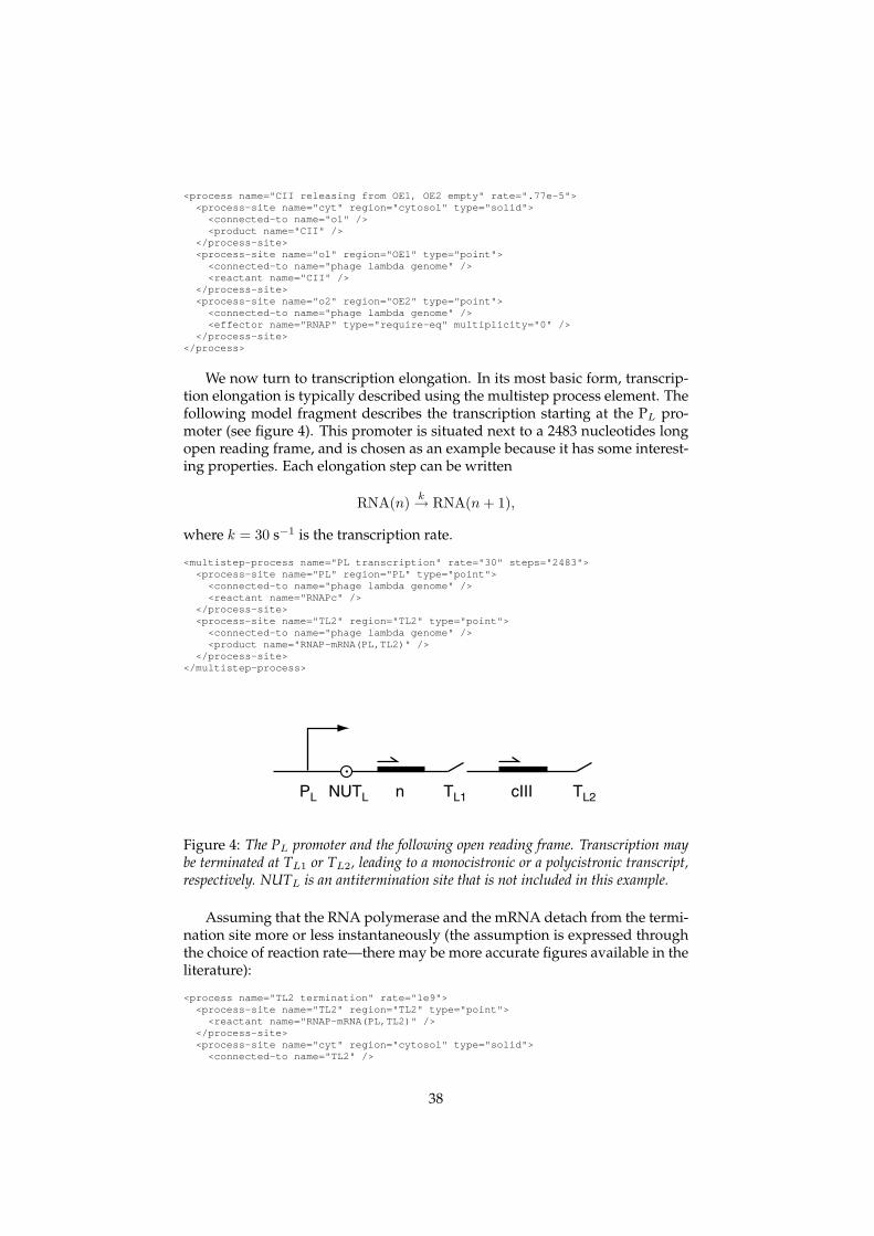
<process name="CII releasing from OE1, OE2 empty" rate=".77e-5"><process-site name="cyt" region="cytosol" type="solid">

<connected-to name="o1" /><product name="CII" />


<connected-to name="phage lambda genome" /><reactant name="CII" />


<connected-to name="phage lambda genome" /><effector name="RNAP" type="require-eq" multiplicity="0" />


We now turn to transcription elongation. In its most basic form, transcrip-tion elongation is typically described using the multistep process element. Thefollowing model fragment describes the transcription starting at the PL pro-moter (see figure 4). This promoter is situated next to a 2483 nucleotides longopen reading frame, and is chosen as an example because it has some interest-ing properties. Each elongation step can be written

RNA(n) k→ RNA(n + 1),

where k = 30 s−1 is the transcription rate.

<multistep-process name="PL transcription" rate="30" steps="2483"><process-site name="PL" region="PL" type="point">

<connected-to name="phage lambda genome" /><reactant name="RNAPc" />

</process-site><process-site name="TL2" region="TL2" type="point">

<connected-to name="phage lambda genome" /><product name="RNAP-mRNA(PL,TL2)" />


PL NUTL n TL1 cIII TL2

Figure 4: The PL promoter and the following open reading frame. Transcription maybe terminated at TL1 or TL2, leading to a monocistronic or a polycistronic transcript,respectively. NUTL is an antitermination site that is not included in this example.

Assuming that the RNA polymerase and the mRNA detach from the termi-nation site more or less instantaneously (the assumption is expressed throughthe choice of reaction rate—there may be more accurate figures available in theliterature):

<process name="TL2 termination" rate="1e9"><process-site name="TL2" region="TL2" type="point">

<reactant name="RNAP-mRNA(PL,TL2)" /></process-site><process-site name="cyt" region="cytosol" type="solid">

<connected-to name="TL2" />

38

<product name="RNAP" /><product name="mRNA(PL,TL2)" />


The PL ORF adds both termination and antitermination to the basic modeof operation. To include termination, the process is split into two: transcriptionupstream and downstream from the termination site. There are two possibleoutcomes from the RNAP-mRNA complex at the termination site: elongationmay continue, resulting in a complete mRNA, or the premature mRNA maybe released. As in the original model, transcription also slows down at thetermination site.

<multistep-process name="PL transcription, part 1" rate="30"steps="2089"><process-site name="PL" region="PL" type="point">

<connected-to name="phage lambda genome" /><reactant name="RNAPc" />




<process name="TL1 termination" rate="25"><process-site name="TL1" region="TL1" type="point">

<connected-to name="phage lambda genome" /><reactant name="RNAP-mRNA(PL,TL1)" />

</process-site><process-site name="cyt" region="cytosol" type="solid">

<connected-to name="TL1" /><product name="RNAP" /><product name="mRNA(PL,TL1)" />


<process name="TL1 elongation" rate="5"><process-site name="TL1" region="TL1" type="point">


</process-site><process-site name="TL1.end" region="TL1.end" type="point">



<multistep-process name="PL transcription, part 2" rate="30" steps="394"><process-site name="TL1.end" region="TL1.end" type="point">





As a matter of fact, the transcription of this particular gene is even morecomplex than this, because it also involves an antitermination process: theRNAP-mRNA complex may be modified at the NUTL site to become “immu-nised” against premature termination at TL1. The implementation of this isnot shown here, but is easily put together using the above concepts. We cantherefore end the transcription submodule:

</module>

39

A.4.5 Translation

The translation of messenger RNA starts immediately after the transcriptionstart, as the ribosomes attach to the free end of mRNA. In the model of Arkinet al, the ribosomes compete for the free end of mRNA with RNAse E. Thereaction rates are related in such a way that an average of ten protein moleculesare synthesised from each transcript, before the transcript is degraded by theRNAse.

It is difficult to implement this exact timing in a Smartcell model. Withthe transcription model described above, there is no way of knowing whena free end is available. The approach taken here is to allow the transcriptionprocess to finish before letting any ribosomes or RNAse molecules attach. Tocompensate for lost translation time, it is then assumed that half of the mRNAhas already been translated when the ribosome attaches. This approximationcertainly has its drawbacks (for example, ribosome crowding is totally ignored)and it may even be totally unacceptable for some applications. There is also aloss of semantics in the model. On the other hand, it does get the averagesright and also the skewed time distributions characteristic of gene expression(McAdams and Arkin, 1997). The competition between translation initiationand mRNA degradation can be formulated as

<process name="mRNA(PL) translation initiation" rate="0.002"><process-site name="cyt" region="cytosol" type="solid">

<reactant name="ribosome" /><effector name="mRNA(PL)" /><product name="ribosome-mRNA(PL)" />


<process name="mRNA(PL) degradation" rate="0.03"><process-site name="cyt" region="cytosol" type="solid">

<reactant name="mRNA(PL)" /><effector name="RNAse E" />


As the rate of the second process is specified in a peculiar way in the origi-nal model, it was assumed that the free concentration of RNAse E is 3 nM in thecytosol. One can then compare the velocities of the two reactions; the velocityof the translation initiation reaction should be ten times that of the degradationreaction, as the average number of transcripts from one mRNA molecule is ten.

Note that the mRNA molecule is removed as soon as the RNAse attaches;this correctly models the function of the system, but may yield strange mRNAconcentration measurements.

The last part of the translation process is the translation elongation, mod-elled as a multistep process, and the (almost instantaneous) dissociation of theribosome from the nascent protein. The rate is 100 amino acids or 33 codonsper second:

<multistep-process name="mRNA(PL) translation elongation" rate="33" steps="66"><process-site name="cyt" region="cytosol" type="solid">

<reactant name="ribosome-mRNA(PL)" /><product name="ribosome-N" />


<process name"ribosome-N dissociation" rate="1e9"><process-site name="cyt" region="cytosol" type="solid">

<reactant name="ribosome-N" />

40

<product name="ribosome" /><product name="N" />


Now this particular mRNA is in fact polycistronic – the gene coding forCIII is on the same mRNA transcript. According to Lewin (2000; p 128) theribosomes do not translate the coding regions of a polycistronic mRNA in se-quence, but release and assemble anew at each start codon. This means that thetranslation of the genes on the same mRNA can be treated as separate processesand one needs only add another multistep process for the CIII translation (notshown here).

This is the end of the model description section, and so we turn to the sim-ulation parameters module.

A.4.6 Cell Growth by Parameter Variation

Cell growth is a fundamental issue for an organism whose life cycle lasts foronly about 35 minutes. The rapid volume expansion means that dilution maybe more important than degradation in regulatory circuits.

In the Arkin et al model, the volume increases linearly from 10−15 L to thedouble volume in 35 minutes. The ideal way of modelling cell growth in theSmartcell environment would be to add more volume elements as time pro-ceeds, but unfortunately this is not yet possible. Instead, one can maintain afixed number of volume elements but increase their size with time. As the ge-ometry model consists of a single cubic volume element, the side of which isthe lattice unit, the lattice unit λ should start out at 1 µm in order to obtain therequired volume. As the volume is proportional to λ3, the expression for thelattice unit looks as follows:

<parameter name="lu">1 + 0.020*tˆ(1/3)</parameter>

A.4.7 Initial Amounts and Constraints

All of the phage lambda gene products start out at zero concentration. There-fore it is not necessary to add initial-amount elements for them, but doing so isgood practice:

<initial-amount name="Cro" region="universe" type="solid">0

</initial-amount>

The initial concentrations for all householding proteins were given in theoriginal paper, so they are also easily added. However in some cases the choicemust be made whether the concentration should be constrained. ConsiderRNAP (RNA polymerase) as an example: even though it is temporarily im-mobilised by certain processes, the effect of the fluctuations is negligible. Onecan therefore put a time-invariant constraint on the concentration at 30 nM,thereby simplifying the model and reducing execution time:

<constraint name="RNAP" region="cytosol" type="solid">30e-9

</constraint>

41

The final example on initial amounts is the MOI (multiplicity of infection),defined as the number of post-infection phage particles in a specific cell. TheMOI is represented in the model by the number of copies of phage DNA. Be-cause each DNA molecule should be mapped to a separate path, a number ofpaths will have to be defined for MOI larger than one. This example showshow a single copy of phage DNA is mapped to an existing path called chromo-some.

<dna-mapping entity="phage lambda genome" region="chromosome" />

It is assumed that infection takes place “early enough” in the cell cycle sothat the phage DNA is present at the start of the cell cycle.

A.4.8 Simulation Output

The interesting outputs from the simulation are the amounts of Cro and CIdimers as functions of time. This information is gathered in the form of twotime series (the interval between samples was arbitrarily chosen to be one sec-ond):

<time-series name="Cro2(t)"entity="Cro2" region="cytosol" type="solid" interval="1" />

<time-series name="CI2(t)"entity="CI2" region="cytosol" type="solid" interval="1" />

That concludes this example. Although not complete and testable, it shouldgive a hint at what can be done and what can not be done with the Smartcellframework.

42

B Mesoscopic Diffusion

In a macroscopic model, the diffusion of an entity in solution is easily expressedas a differential equation, and added to the system of coupled differential equa-tions that describe the interactions between species. Diffusion across bound-aries or along paths is handled in much the same way. This is not quite thecase for stochastic kinetics. In this appendix a new method for introducingdiffusion into a mesoscopic model is presented.

To start with, let us take a look at the macroscopic diffusion equation. Ina macroscopic model, the concentration C of some species is assumed to becontinuous in space. Consider a small volume element δV which is centred atr. There are several factors contributing to the flux of matter in and out of thisvolume element. Let S(r) denote the amount of species that is created in δVper unit time and volume (S may of course assume negative values as well).We also introduce the flux, denoted by j(r). These quantities are related by acontinuity relation,

∫∫∫

δV

∂C

∂tdV =

∫∫∫

δV

SdV −∫∫

∂δV

j · dS (11)

Applying Gauss’ theorem yields∫∫∫

δV

∂C

∂tdV =

∫∫∫

δV

SdV −∫∫∫

δV

∇ · j dV (12)

In the limit of vanishingly small δV , the equation becomes exact in the in-tegrands and reads ∂C/∂t = S − ∇ · j. The factors contributing to the fluxare:

diffusion. Fick’s law states that the diffusion flux jD = −D∇C. Here, D is thediffusion constant and C is the concentration.

ion drift due to electrostatic fields. Ionic species have a drift speed s, whichgives rise to an ion flux jE = −sC. The drift speed is related to theelectric field by the relation s = uE, and the ion mobility u is in turn givenby the Einstein relation u = zDe/kBT . Here, z is the ionic valence, e isthe elementary charge, kB is Bolzmann’s constant and T is the absolutetemperature. This leads to the equation jE = −zDeCE/kBT . See Atkins(1994) for a more detailed descriptions of these relations.

convection due temperature gradients, stirring, etc. The convective flux is gi-ven by jC = −vC, where v is the velocity field.

By superposition we arrive at an expression for ji that, through the introduc-tion of the constants ai and bi, can be written

ji = −a∇C − bC. (13)

The mesoscopic flux is neither space-continuous nor time-continuous. Ra-ther, it is a stochastic event; a transient movement of entities between neigh-bour sites. What is the propensity of such an event? We focus on one of thesites, say u (see figure 5), and try to find the escape probability εuv , defined as

43

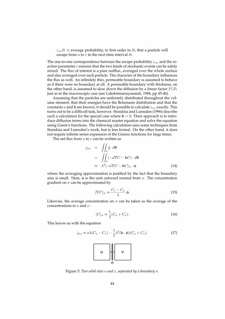
εuvδt ≡ average probability, to first order in δt, that a particle willescape from u to v in the next time interval δt.

The one-to-one correspondence between the escape probability εuv and the re-action parameter c ensures that the two kinds of stochastic events can be safelymixed. The flux of interest is a pure outflux, averaged over the whole surfaceand also averaged over each particle. The character of the boundary influencesthe flux as well. An infinitely thin, permeable boundary is assumed to behaveas if there were no boundary at all. A permeable boundary with thickness, onthe other hand, is assumed to slow down the diffusion by a linear factor P/D,just as in the macroscopic case (see Lakshminarayanaiah, 1984, pp 45-46).

Assuming that the particles are uniformly distributed throughout the vol-ume element, that their energies have the Bolzmann distribution and that theconstants a and b are known, it should be possible to calculate εuv exactly. Thisturns out to be a difficult task, however. Stundzia and Lumsden (1996) describesuch a calculation for the special case where b = 0. Their approach is to intro-duce diffusion terms into the chemical master equation and solve the equationusing Green’s functions. The following calculation uses some techniques fromStundzia and Lumsden’s work, but is less formal. On the other hand, it doesnot require infinite series expansion of the Greens functions for large times.

The net flux from u to v can be written as

juv =∫∫

σ

j · dS

=∫∫

σ

(−a∇C − bC) · dS

≈ λ2〈−a∇C − bC〉σ · n (14)

where the averaging approximation is justified by the fact that the boundaryarea is small. Here, n is the unit outward normal from u. The concentrationgradient on σ can be approximated by

〈∇C〉σ ≈ Cv − Cu

λn. (15)

Likewise, the average concentration on σ can be taken as the average of theconcentrations in u and v:

〈C〉σ ≈ 12(Cu + Cv). (16)

This leaves us with the equation

juv ≈ aλ(Cu − Cv)− 12λ2(b · n)(Cu + Cv). (17)

Figure 5: Two solid sites u and v, separated by a boundary σ.

44

Back in the mesoscopic model, each particle in u has the probability εuv ofescaping to v in the next unit time interval. These events are independent, soan average of Xuεuv particles will escape per time unit. The reverse processtakes place simultaneously in v, leading to an average net flux Xuεuv −Xvεvu

from u to v. For reasons of consistency, we require that this average net flux beequal to the juv calculated above. Therefore, by identification,

εuv =Cu

Xu(aλ− 1

2λ2(b · n))

=a

NAλ2− b · n

2NAλ(18)

It should be noted that n is the outward unit normal relative to each volumeelement, so that nv = −nu.

A similar calculation for the two-dimensional case gives exactly the sameresult. With this expression, a diffusion movement will be present even if theconcentrations in the neighbour sites are equal, as opposed to the situationin deterministic models. The stochastic model comes closer to the thermody-namic character of diffusion—including interesting fluctuation phenomena—but it may do so at the cost of a higher computational load.

If the external fields are very strong, εuv may become negative. To preventthis unphysical condition, the lattice unit must be chosen small enough so thatat all times

λ ≤ 2a

|b · n| . (19)

However, it is very unlikely that any external fields will be included into themodel. The electrostatic interaction will be very weak in the solvent, due to thescreening effect of the water (according to Luis Serrano). But a strong electricpotential can be maintained across membranes, so it could be useful in thiscase. A model of a calcium wave in a neuronal cell, that includes a membranepotential, is described in Schaff et al (1997).

45

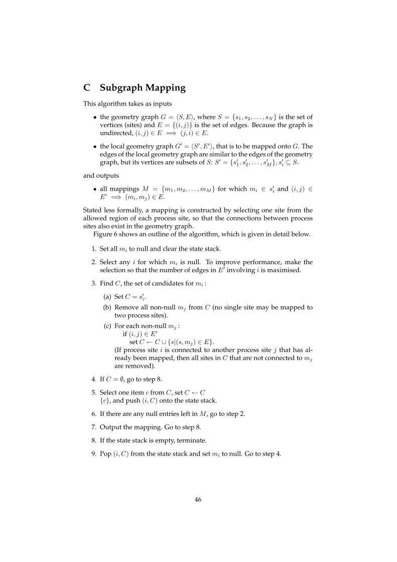
C Subgraph Mapping

This algorithm takes as inputs

• the geometry graph G = 〈S, E〉, where S = {s1, s2, . . . , sN} is the set ofvertices (sites) and E = {(i, j)} is the set of edges. Because the graph isundirected, (i, j) ∈ E =⇒ (j, i) ∈ E.

• the local geometry graph G′ = 〈S′, E′〉, that is to be mapped onto G. Theedges of the local geometry graph are similar to the edges of the geometrygraph, but its vertices are subsets of S: S′ = {s′1, s′2, . . . , s′M}, s′i ⊆ S.

and outputs

• all mappings M = {m1,m2, . . . , mM} for which mi ∈ s′i and (i, j) ∈E′ =⇒ (mi, mj) ∈ E.

Stated less formally, a mapping is constructed by selecting one site from theallowed region of each process site, so that the connections between processsites also exist in the geometry graph.

Figure 6 shows an outline of the algorithm, which is given in detail below.

1. Set all mi to null and clear the state stack.

2. Select any i for which mi is null. To improve performance, make theselection so that the number of edges in E′ involving i is maximised.

3. Find C, the set of candidates for mi :

(a) Set C = s′i.

(b) Remove all non-null mj from C (no single site may be mapped totwo process sites).

(c) For each non-null mj :if (i, j) ∈ E′

set C ← C ∪ {s|(s,mj) ∈ E}.(If process site i is connected to another process site j that has al-ready been mapped, then all sites in C that are not connected to mj

are removed).

4. If C = ∅, go to step 8.

5. Select one item c from C, set C ← C{c}, and push (i, C) onto the state stack.

6. If there are any null entries left in M , go to step 2.

7. Output the mapping. Go to step 8.

8. If the state stack is empty, terminate.

9. Pop (i, C) from the state stack and set mi to null. Go to step 4.

46

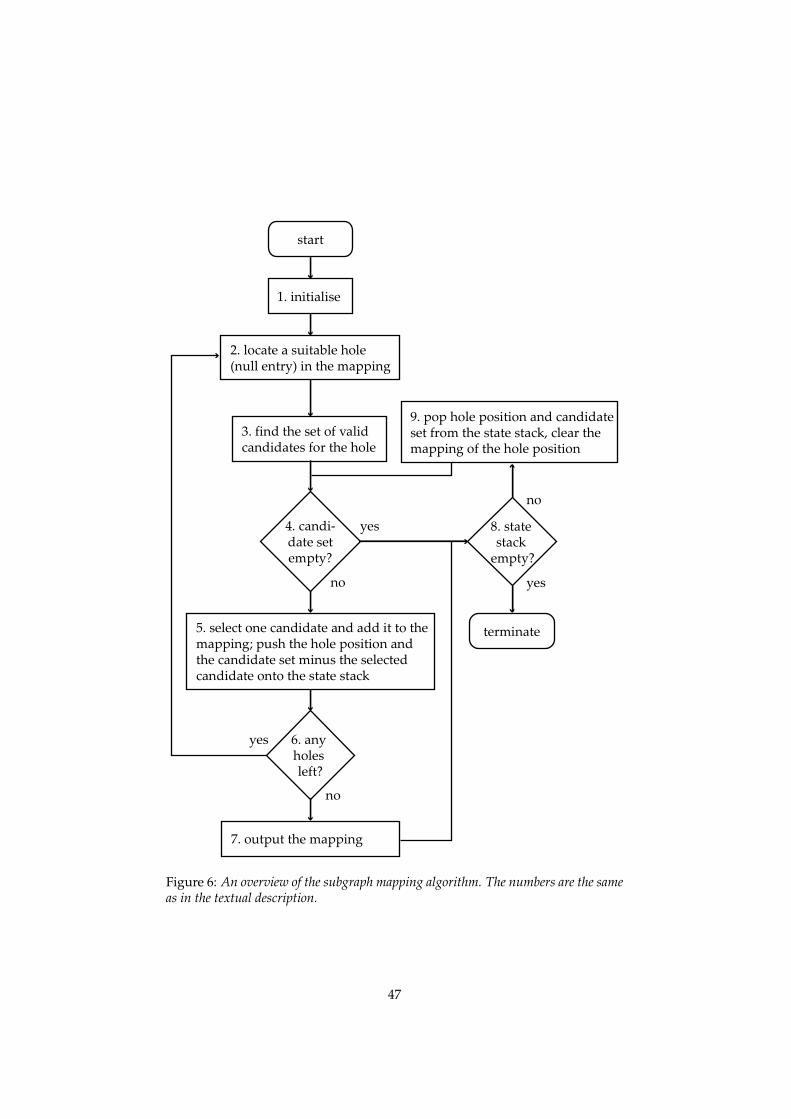
Figure 6: An overview of the subgraph mapping algorithm. The numbers are the sameas in the textual description.

47

anders kaplan - uppsala university

Documents