and/or multi-valued decision diagrams (aomdds) for ... · and/or multi-valued decision diagrams...
TRANSCRIPT

Journal of Artificial Intelligence Research 33 (2008) 465-519 Submitted 05/08; published 12/08
AND/OR Multi-Valued Decision Diagrams (AOMDDs)for Graphical Models
Robert Mateescu [email protected] Engineering DepartmentCalifornia Institute of TechnologyPasadena, CA 91125, USA
Rina Dechter [email protected] Bren School of Information and Computer ScienceUniversity of California IrvineIrvine, CA 92697, USA
Radu Marinescu [email protected] Constraint Computation CentreUniversity College Cork, Ireland
AbstractInspired by the recently introduced framework of AND/OR search spaces for graphical mod-
els, we propose to augment Multi-Valued Decision Diagrams (MDD) with AND nodes, in orderto capture function decomposition structure and to extend these compiled data structures to gen-eral weighted graphical models (e.g., probabilistic models). We present the AND/OR Multi-ValuedDecision Diagram (AOMDD) which compiles a graphical model into a canonical form that sup-ports polynomial (e.g., solution counting, belief updating) or constant time (e.g. equivalence ofgraphical models) queries. We provide two algorithms for compiling the AOMDD of a graphicalmodel. The first is search-based, and works by applying reduction rules to the trace of the memoryintensive AND/OR search algorithm. The second is inference-based and uses a Bucket Eliminationschedule to combine the AOMDDs of the input functions via the the APPLY operator. For bothalgorithms, the compilation time and the size of the AOMDD are, in the worst case, exponential inthe treewidth of the graphical model, rather than pathwidth as is known for ordered binary decisiondiagrams (OBDDs). We introduce the concept of semantic treewidth, which helps explain whythe size of a decision diagram is often much smaller than the worst case bound. We provide anexperimental evaluation that demonstrates the potential of AOMDDs.
1. Introduction
The paper extends decision diagrams into AND/OR multi-valued decision diagrams (AOMDDs)and shows how graphical models can be compiled into these data-structures. The work presented inthis paper is based on two existing frameworks: (1) AND/OR search spaces for graphical modelsand (2) decision diagrams.
1.1 AND/OR Search Spaces
AND/OR search spaces (Dechter & Mateescu, 2004a, 2004b, 2007) have proven to be a unifyingframework for various classes of search algorithms for graphical models. The main characteristic isthe exploitation of independencies between variables during search, which can provide exponentialspeedups over traditional search methods that can be viewed as traversing an OR structure. The
c©2008 AI Access Foundation. All rights reserved.

MATEESCU, DECHTER & MARINESCU
AND nodes capture problem decomposition into independent subproblems, and the OR nodes rep-resent branching according to variable values. AND/OR spaces can accommodate dynamic variableordering, however most of the current work focuses on static decomposition. Examples of AND/ORsearch trees and graphs will appear later, for example in Figures 6 and 7.The AND/OR search space idea was originally developed for heuristic search (Nilsson, 1980).
In the context of graphical models, AND/OR search (Dechter & Mateescu, 2007) was also inspiredby search advances introduced sporadically in the past three decades for constraint satisfaction andmore recently for probabilistic inference and for optimization tasks. Specifically, it resembles thepseudo tree rearrangement (Freuder & Quinn, 1985, 1987), that was adapted subsequently for dis-tributed constraint satisfaction by Collin, Dechter, and Katz (1991, 1999) and more recently byModi, Shen, Tambe, and Yokoo (2005), and was also shown to be related to graph-based backjump-ing (Dechter, 1992). This work was extended by Bayardo and Miranker (1996) and Bayardo andSchrag (1997) and more recently applied to optimization tasks by Larrosa, Meseguer, and Sanchez(2002). Another version that can be viewed as exploring the AND/OR graphs was presented re-cently for constraint satisfaction (Terrioux & Jegou, 2003b) and for optimization (Terrioux & Jegou,2003a). Similar principles were introduced recently for probabilistic inference, in algorithm Recur-sive Conditioning (Darwiche, 2001) as well as in Value Elimination (Bacchus, Dalmao, & Pitassi,2003b, 2003a), and are currently at the core of the most advanced SAT solvers (Sang, Bacchus,Beame, Kautz, & Pitassi, 2004).
1.2 Decision Diagrams
Decision diagrams are widely used in many areas of research, especially in software and hardwareverification (Clarke, Grumberg, & Peled, 1999; McMillan, 1993). A BDD represents a Booleanfunction by a directed acyclic graph with two terminal nodes (labeled 0 and 1), and every internalnode is labeled with a variable and has exactly two children: low for 0 and high for 1. If isomorphicnodes were not merged, we would have the full search tree, also called Shannon tree, which is theusual full tree explored by a backtracking algorithm. The tree is ordered if variables are encounteredin the same order along every branch. It can then be compressed by merging isomorphic nodes(i.e., with the same label and identical children), and by eliminating redundant nodes (i.e., whoselow and high children are identical). The result is the celebrated reduced ordered binary decisiondiagram, or OBDD for short, introduced by Bryant (1986). However, the underlying structure isOR, because the initial Shannon tree is an OR tree. If AND/OR search trees are reduced by nodemerging and redundant nodes elimination we get a compact search graph that can be viewed as aBDD representation augmented with AND nodes.
1.3 Knowledge Compilation for Graphical Models
In this paper we combine the two ideas, creating a decision diagram that has an AND/OR struc-ture, thus exploiting problem decomposition. As a detail, the number of values is also increasedfrom two to any constant. In the context of constraint networks, decision diagrams can be used torepresent the whole set of solutions, facilitating solutions count, solution enumeration and querieson equivalence of constraint networks. The benefit of moving from OR structure to AND/OR is ina lower complexity of the algorithms and size of the compiled structure. It typically moves frombeing bounded exponentially in pathwidth pw∗, which is characteristic to chain decompositions orlinear structures, to being exponentially bounded in treewidth w∗, which is characteristic of tree
466

AND/OR MULTI-VALUED DECISION DIAGRAMS (AOMDDS) FOR GRAPHICAL MODELS
structures (Bodlaender & Gilbert, 1991) (it always holds that w∗ ≤ pw∗ and pw∗ ≤ w∗ · log n,where n is the number of variables of the model). In both cases, the compactness result achieved inpractice is often far smaller than what the bounds suggest.A decision diagram offers a compilation of a propositional knowledge-base. An extension of
the OBDDs was provided by Algebraic Decision Diagrams (ADD) (Bahar, Frohm, Gaona, Hachtel,Macii, Pardo, & Somenzi, 1993), where the terminal nodes are not just 0 or 1, but take values froman arbitrary finite domain. The knowledge compilation approach has become an important researchdirection in automated reasoning in the past decade (Selman & Kautz, 1996; Darwiche & Marquis,2002; Cadoli & Donini, 1997). Typically, a knowledge representation language is compiled into acompact data structure that allows fast responses to various queries. Accordingly, the computationaleffort can be divided between an offline and an online phase where most of the work is pushedoffline. Compilation can also be used to generate compact building blocks to be used by onlinealgorithms multiple times. Macro-operators compiled during or prior to search can be viewed inthis light (Korf & Felner, 2002), while in graphical models the building blocks are the functionswhose compact compiled representations can be used effectively across many tasks.As one example, consider product configuration tasks and imagine a user that chooses sequen-
tial options to configure a product. In a naive system, the user would be allowed to choose any validoption at the current level based only on the initial constraints, until either the product is configured,or else, when a dead-end is encountered, the system would backtrack to some previous state andcontinue from there. This would in fact be a search through the space of possible partial config-urations. Needless to say, it would be very unpractical, and would offer the user no guarantee offinishing in a limited time. A system based on compilation would actually build the backtrack-freesearch space in the offline phase, and represent it in a compact manner. In the online phase, onlyvalid partial configurations (i.e., that can be extended to a full valid configuration) are allowed, anddepending on the query type, response time guarantees can be offered in terms of the size of thecompiled structure.Numerous other examples, such as diagnosis and planning problems, can be formulated as
graphical models and could benefit from compilation (Palacios, Bonet, Darwiche, & Geffner, 2005;Huang & Darwiche, 2005a). In diagnosis, compilation can facilitate fast detection of possible faultsor explanations for some unusual behavior. Planning problems can also be formulated as graphicalmodels, and a compilation would allow swift adjustments according to changes in the environment.Probabilistic models are one of the most used types of graphical models, and the basic query is tocompute conditional probabilities of some variables given the evidence. A compact compilation of aprobabilistic model would allow fast response to queries that incorporate evidence acquired in time.For example, two of the most important tasks for Bayesian networks are computing the probabilityof the evidence, and computing the maximum probable explanation (MPE). If some of the modelvariables become assigned (evidence), these tasks can be performed in time linear in the compila-tion size, which in practice is in many cases smaller than the upper-bound based on the treewidth orpathwidth of the graph. Formal verification is another example where compilation is heavily usedto compare equivalence of circuit design, or to check the behavior of a circuit. Binary DecisionDiagram (BDD) (Bryant, 1986) is arguably the most widely known and used compiled structure.The contributions made in this paper to knowledge compilation in general and to decision dia-
grams in particular are the following:
1. We formally describe the AND/OR Multi-Valued Decision Diagram (AOMDD) and prove itto be a canonical representation for constraint networks, given a pseudo tree.
467
MATEESCU, DECHTER & MARINESCU
2. We extend the AOMDD to general weighted graphical models.
3. We give a compilation algorithm based on AND/OR search, that saves the trace of a memoryintensive search and then reduces it in one bottom up pass.
4. We present the APPLY operator that combines two AOMDDs and show that its complexity isat most quadratic in the input, but never worse than exponential in the treewidth.
5. We give a scheduling order for building the AOMDD of a graphical model starting withthe AOMDDs of its functions which is based on a Variable Elimination algorithm. Thisguarantees that the complexity is at most exponential in the induced width (treewidth) alongthe ordering.
6. We show how AOMDDs relate to various earlier and recent compilation frameworks, provid-ing a unifying perspective for all these methods.
7. We introduce the semantic treewidth, which helps explain why compiled decision diagramsare often much smaller than the worst case bound.
8. We provide an experimental evaluation of the new data structure.
The structure of the paper is as follows. Section 2 provides preliminary definitions, a descriptionof binary decision diagrams and the Bucket Elimination algorithm. Section 3 gives an overview ofAND/OR search spaces. Section 4 introduces the AOMDD and discusses its properties. Section5 describes a search-based algorithm for compiling the AOMDD. Section 6 presents a compilationalgorithm based on a Bucket Elimination schedule and the APPLY operation. Section 7 proves thatthe AOMDD is a canonical representation for constraint networks given a pseudo tree, and Section8 extends the AOMDD to weighted graphical models and proves their canonicity. Section 9 tiesthe canonicity to the new concept of semantic treewidth. Section 10 provides an experimentalevaluation. Section 11 presents related work and Section 12 concludes the paper. All the proofsappear in an appendix.
2. Preliminaries
Notations A reasoning problem is defined in terms of a set of variables taking values from finitedomains and a set of functions defined over these variables. We denote variables or subsets ofvariables by uppercase letters (e.g., X, Y, . . .) and values of variables by lower case letters (e.g.,x, y, . . .). Sets are usually denoted by bold letters, for example X = {X1, . . . , Xn} is a set ofvariables. An assignment (X1 = x1, . . . , Xn = xn) can be abbreviated as x = (〈X1, x1〉, . . . ,〈Xn, xn〉) or x = (x1, . . . , xn). For a subset of variables Y, DY denotes the Cartesian product ofthe domains of variables in Y. The projection of an assignment x = (x1, . . . , xn) over a subset Yis denoted by xY or x[Y]. We will also denote by Y = y (or y for short) the assignment of valuesto variables inY from their respective domains. We denote functions by letters f , g, h etc., and thescope (set of arguments) of the function f by scope(f).
2.1 Graphical Models
DEFINITION 1 (graphical model) A graphical modelM is a 4-tuple,M = 〈X,D,F,⊗〉, where:
468

AND/OR MULTI-VALUED DECISION DIAGRAMS (AOMDDS) FOR GRAPHICAL MODELS
1. X = {X1, . . . , Xn} is a finite set of variables;2. D = {D1, . . . , Dn} is the set of their respective finite domains of values;3. F = {f1, . . . , fr} is a set of positive real-valued discrete functions (i.e., their domains canbe listed), each defined over a subset of variables Si ⊆ X, called its scope, and denoted byscope(fi).
4. ⊗ is a combination operator1 (e.g., ⊗ ∈ {∏
,∑
, �} – product, sum, join), that can take asinput two (or more) real-valued discrete functions, and produce another real-valued discretefunction.
The graphical model represents the combination of all its functions: ⊗ri=1fi.
Several examples of graphical models appear later, for example: Figure 1 shows a constraintnetwork and Figure 2 shows a belief network.In order to define the equivalence of graphical models, it is useful to introduce the notion of
universal graphical model that is defined by a single function.
DEFINITION 2 (universal equivalent graphical model) Given a graphical model M =〈X,D,F1,⊗〉 the universal equivalent model ofM is u(M) = 〈X,D,F2 = {⊗fi∈F1fi},⊗〉.
Two graphical models are equivalent if they represent the same function. Namely, if they havethe same universal model.
DEFINITION 3 (weight of a full and a partial assignment) Given a graphical model M =〈X,D,F〉, the weight of a full assignment x = (x1, . . . , xn) is defined by w(x) =⊗f∈Ff(x[scope(f)]). Given a subset of variables Y ⊆ X, the weight of a partial assignmenty is the combination of all the functions whose scopes are included inY (denoted by FY) evaluatedat the assigned values. Namely, w(y) = ⊗f∈FY
f(y[scope(f)]).
Consistency For most graphical models, the range of the functions has a special zero value “0”that is absorbing relative to the combination operator (e.g., multiplication). Combining anythingwith “0” yields a “0”. The “0” value expresses the notion of inconsistent assignments. It is a primaryconcept in constraint networks but can also be defined relative to other graphical models that have a“0” element.
DEFINITION 4 (consistent partial assignment, solution) Given a graphical model having a “0”element, a partial assignment is consistent if its cost is non-zero. A solution is a consistent assign-ment to all the variables.
DEFINITION 5 (primal graph) The primal graph of a graphical model is an undirected graph thathas variables as its vertices and an edge connects any two variables that appear in the scope of thesame function.
The primal graph captures the structure of the knowledge expressed by the graphical model. Inparticular, graph separation indicates independency of sets of variables given some assignments toother variables. All of the advanced algorithms for graphical models exploit the graphical structure,by using a heuristically good elimination order, a tree decomposition or some similar method. Wewill use the concept of pseudo tree, which resembles the tree rearrangements introduced by Freuderand Quinn (1985):
1. The combination operator can also be defined axiomatically (Shenoy, 1992).
469

MATEESCU, DECHTER & MARINESCU
C
A
B
D
E
F
G
(a) Graph coloring problem
A
BD
CG
F
E
(b) Constraint graph
Figure 1: Constraint network
DEFINITION 6 (pseudo tree) A pseudo tree of a graph G = (X, E) is a rooted tree T having thesame set of nodesX, such that every arc in E is a backarc in T (A path in a rooted tree starts at theroot and ends at one leaf. Two nodes can be connected by a backarc only if there exists a path thatcontains both).
We use the common concepts and parameters from graph theory, that characterize the connec-tivity of the graph, and how close it is to a tree or to a chain. The induced width of a graphical modelgoverns the complexity of solving it by Bucket Elimination (Dechter, 1999), and was also shown tobound the AND/OR search graph when memory is used to cache solved subproblems (Dechter &Mateescu, 2007).
DEFINITION 7 (induced graph, induced width, treewidth, pathwidth) An ordered graph is apair (G, d), where G = ({X1, . . . , Xn}, E) is an undirected graph, and d = (X1, . . . , Xn) is anordering of the nodes. The width of a node in an ordered graph is the number of neighbors thatprecede it in the ordering. The width of an ordering d, denoted w(d), is the maximum width overall nodes. The induced width of an ordered graph, w∗(d), is the width of the induced ordered graphobtained as follows: for each node, from last to first in d, its preceding neighbors are connectedin a clique. The induced width of a graph, w∗, is the minimal induced width over all orderings.The induced width is also equal to the treewidth of a graph. The pathwidth pw∗ of a graph is thetreewidth over the restricted class of orderings that correspond to chain decompositions.
Various reasoning tasks, or queries can be defined over graphical models. Those can be de-fined formally using marginalization operators such as projection, summation and minimization.However, since our goal is to present a compilation of a graphical model which is independent ofthe queries that can be posed on it, we will discuss tasks in an informal manner only. For moreinformation see the work of Kask, Dechter, Larrosa, and Dechter (2005).Throughout the paper, we will use two examples of graphical models: constraint networks
and belief networks. In the case of constraint networks, the functions can be understood as rela-tions. In other words, the functions (also called constraints) can take only two values, {0, 1}, or{false, true}. A 0 value indicates that the corresponding assignment to the variables is inconsis-tent (not allowed), and a 1 value indicates consistency. Belief networks are an example of the moregeneral case of graphical models (also called weighted graphical models). The functions in this caseare conditional probability tables, so the values of a function are real numbers in the interval [0, 1].
470

AND/OR MULTI-VALUED DECISION DIAGRAMS (AOMDDS) FOR GRAPHICAL MODELS
Example 1 Figure 1(a) shows a graph coloring problem that can be modeled by a constraint net-work. Given a map of regions, the problem is to color each region by one of the given colors {red,green, blue}, such that neighboring regions have different colors. The variables of the problemsare the regions, and each one has the domain {red, green, blue}. The constraints are the relation“different” between neighboring regions. Figure 1(b) shows the constraint graph, and a solution(A=red, B=blue, C=green, D=green, E=blue, F=blue, G=red) is given in Figure 1(a). A moredetailed example will be given later in Example 8.
Propositional Satisfiability A special case of a CSP is propositional satisfiability (SAT). A for-mula ϕ in conjunctive normal form (CNF) is a conjunction of clauses α1, . . . , αt, where a clauseis a disjunction of literals (propositions or their negations). For example, α = (P ∨ ¬Q ∨ ¬R) isa clause, where P , Q and R are propositions, and P , ¬Q and ¬R are literals. The SAT problemis to decide whether a given CNF theory has a model, i.e., a truth-assignment to its propositionsthat does not violate any clause. Propositional satisfiability (SAT) can be defined as a CSP, wherepropositions correspond to variables, domains are {0, 1}, and constraints are represented by clauses,for example the clause (¬A ∨ B) is a relation over its propositional variables that allows all tuplesover (A, B) except (A = 1, B = 0).
Cost Networks An immediate extension of constraint networks are cost networks where the setof functions are real-valued cost functions, and the primary task is optimization. Also, GAI-nets(generalized additive independence, Fishburn, 1970) can be used to represent utility functions. Anexample of cost functions will appear in Figure 19.
DEFINITION 8 (cost network, combinatorial optimization) A cost network is a 4-tuple,〈X,D,C,
∑〉, where X is a set of variables X = {X1, . . . , Xn}, associated with a set of
discrete-valued domains,D = {D1, . . . , Dn}, and a set of cost functionsC = {C1, . . . , Cr}. EachCi is a real-valued function defined on a subset of variables Si ⊆ X. The combination operator, is∑. The reasoning problem is to find a minimum cost solution.
Belief Networks (Pearl, 1988) provide a formalism for reasoning about partial beliefs under condi-tions of uncertainty. They are defined by a directed acyclic graph over vertices representing randomvariables of interest (e.g., the temperature of a device, the gender of a patient, a feature of an ob-ject, the occurrence of an event). The arcs signify the existence of direct causal influences betweenlinked variables quantified by conditional probabilities that are attached to each cluster of parents-child vertices in the network.
DEFINITION 9 (belief networks) A belief network (BN) is a graphical modelP = 〈X,D,PG,∏〉,
where X = {X1, . . . , Xn} is a set of variables over domains D = {D1, . . . , Dn}. Given a di-rected acyclic graph G over X as nodes, PG = {P1, . . . , Pn}, where Pi = {P (Xi | pa (Xi) ) }are conditional probability tables (CPTs for short) associated with each Xi, where pa(Xi) are theparents ofXi in the acyclic graph G. A belief network represents a probability distribution overX,P (x1, . . . , xn) =
∏ni=1 P (xi|xpa(Xi)). An evidence set e is an instantiated subset of variables.
When formulated as a graphical model, functions in F denote conditional probability tablesand the scopes of these functions are determined by the directed acyclic graph G: each functionfi ranges over variable Xi and its parents in G. The combination operator is product, ⊗ =
∏.
The primal graph of a belief network (viewed as an undirected model) is called a moral graph. Itconnects any two variables appearing in the same CPT.
471

MATEESCU, DECHTER & MARINESCU
A
F
B C
D
G
Season
Sprinkler Rain
Watering Wetness
Slippery
(a) Directed acyclic graph
A
F
B C
D
G
(b) Moral graph
Figure 2: Belief network
Example 2 Figure 2(a) gives an example of a belief network over 6 variables, and Figure 2(b)shows its moral graph . The example expresses the causal relationship between variables “Season”(A), “The configuration of an automatic sprinkler system” (B), “The amount of rain expected”(C), “The amount of manual watering necessary” (D), “The wetness of the pavement” (F ) and“Whether or not the pavement is slippery” (G). The belief network expresses the probability dis-tribution P (A, B, C, D, F, G) = P (A) · P (B|A) · P (C|A) · P (D|B, A) · P (F |C, B) · P (G|F ).Another example of a belief network and CPTs appears in Figure 9.
The two most popular tasks for belief networks are defined below:
DEFINITION 10 (belief updating, most probable explanation (MPE)) Given a belief networkand evidence e, the belief updating task is to compute the posterior marginal probability of variableXi, conditioned on the evidence. Namely,
Bel(Xi = xi) = P (Xi = xi | e) = α∑
{(x1,...,xi−1,xi+1,...,xn)|E=e,Xi=xi}
n∏k=1
P (xk, e|xpak),
where α is a normalization constant. The most probable explanation (MPE) task is to find acomplete assignment which agrees with the evidence, and which has the highest probability amongall such assignments. Namely, to find an assignment (xo
1, . . . , xon) such that
P (xo1, . . . , x
on) = maxx1,...,xn
n∏k=1
P (xk, e|xpak).
2.2 Binary Decision Diagrams Review
Decision diagrams are widely used in many areas of research to represent decision processes. Inparticular, they can be used to represent functions. Due to the fundamental importance of Booleanfunctions, a lot of effort has been dedicated to the study of Binary Decision Diagrams (BDDs),which are extensively used in software and hardware verification (Clarke et al., 1999; McMillan,1993). The earliest work on BDDs is due to Lee (1959), who introduced the binary-decision pro-gram, that can be understood as a linear representation of a BDD (e.g., a depth first search orderingof the nodes), where each node is a branching instruction indicating the address of the next instruc-tion for both the 0 and the 1 value of the test variable. Akers (1978) presented the actual graphical
472

AND/OR MULTI-VALUED DECISION DIAGRAMS (AOMDDS) FOR GRAPHICAL MODELS
11110011110100011110001001000000
f(ABC)CBA
(a) Table
B
A
C
0 0
C
0 1
C
B
0 0
B
1 1
(b) Unordered tree
B
A
C
0 0
C
0 1
B
C
0 1
C
0 1
(c) Ordered tree
Figure 3: Boolean function representations
representation and further developed the BDD idea. However, it was Bryant (1986) that introducedwhat is now called the Ordered Binary Decision Diagram (OBDD). He restricted the order of vari-ables along any path of the diagram, and presented algorithms (most importantly the apply proce-dure, that combines two OBDDs by an operation) that have time complexity at most quadratic in thesizes of the input diagrams. OBDDs are fundamental for applications with large binary functions,especially because in many practical cases they provide very compact representations.A BDD is a representation of a Boolean function. Given B = {0, 1}, a Boolean function
f : Bn → B, has n arguments, X1, · · · , Xn, which are Boolean variables, and takes Boolean
values.
Example 3 Figure 3(a) shows a table representation of a Boolean function of three variables. Thisexplicit representation is the most straightforward, but also the most costly due to its exponentialrequirements. The same function can also be represented by a binary tree, shown in Figure 3(b),that has the same exponential size in the number of variables. The internal round nodes representthe variables, the solid edges are the 1 (or high) value, and the dotted edges are the 0 (or low) value.The leaf square nodes show the value of the function for each assignment along a path. The treeshown in 3(b) is unordered, because variables do not appear in the same order along each path.
In building an OBDD, the first condition is to have variables appear in the same order (A,B,C)along every path from root to leaves. Figure 3(c) shows an ordered binary tree for our function.Once an order is imposed, there are two reduction rules that transform a decision diagram into anequivalent one:(1) isomorphism: merge nodes that have the same label and the same children.(2) redundancy: eliminate nodes whose low and high edges point to the same node, and connectparent of removed node directly to child of removed node.Applying the two reduction rules exhaustively yields a reduced OBDD, sometimes denoted
rOBDD. We will just use OBDD and assume that it is completely reduced.
Example 4 Figure 4(a) shows the binary tree from Figure 3(c) after the isomorphic terminal nodes(leaves) have been merged. The highlighted nodes, labeled with C, are also isomorphic, and Figure4(b) shows the result after they are merged. Now, the highlighted nodes labeled with C and B areredundant, and removing them gives the OBDD in Figure 4(c).
2.3 Bucket Elimination Review
Bucket Elimination (BE) (Dechter, 1999) is a well known variable elimination algorithm for infer-ence in graphical models. We will describe it using the terminology for constraint networks, but BE
473

MATEESCU, DECHTER & MARINESCU
B
A
C C
0 1
B
C C
(a) Isomorphic nodes
B
A
C
0 1
B
C
(b) Redundant nodes
B
A
0 1
C
(c) OBDD
Figure 4: Reduction rules
A
D
B C
E
C3(ABE)
C2(AB)
C4(BCD)
C1(AC)
(a) Constraint network
D: C4 (BCD)
C: C1(AC) h1(BC)
E: C3(ABE)
B: C2(AB) h3(AB) h2(AB)
A: h4(A)
(b) BE execution
A
BCD
AB
ABCABE
A
AB
BC
AB
bucket-A
bucket-E
bucket-B
bucket-C
bucket-D
(c) Bucket tree
Figure 5: Bucket Elimination
can also be applied to any graphical model. Consider a constraint network R = 〈X,D,C〉 and anordering d = (X1, X2, . . . , Xn). The ordering d dictates an elimination order for BE, from last tofirst. Each variable is associated with a bucket. Each constraint fromC is placed in the bucket of itslatest variable in d. Buckets are processed from Xn to X1 by eliminating the bucket variable (theconstraints residing in the bucket are joined together, and the bucket variable is projected out) andplacing the resulting constraint (also called message) in the bucket of its latest variable in d. Afterits execution, BE renders the network backtrack free, and a solution can be produced by assigningvariables along d. BE can also produce the solutions count if marginalization is done by summation(rather than projection) over the functional representation of the constraints, and join is substitutedby multiplication.BE also constructs a bucket tree, by linking the bucket of each Xi to the destination bucket of
its message (called the parent bucket). A node in the bucket tree typically has a bucket variable, acollection of constraints, and a scope (the union of the scopes of its constraints). If the nodes of thebucket tree are replaced by their respective bucket variables, it is easy to see that we obtain a pseudotree.
Example 5 Figure 5(a) shows a network with four constraints. Figure5(b) shows the execution ofBucket Elimination along d = (A, B, E, C, D). The buckets are processed from D to A.2 Figure5(c) shows the bucket tree. The pseudo tree corresponding to the order d is given in Fig. 6(a).
2. The representation in Figure 5 reverses the top down bucket processing described in earlier papers (Dechter, 1999).
474

AND/OR MULTI-VALUED DECISION DIAGRAMS (AOMDDS) FOR GRAPHICAL MODELS
Procedure GeneratePseudoTree(G, d)input : graph G = (X, E); order d = (X1, . . . , Xn)output : Pseudo tree TMakeX1 the root of T1Condition onX1 (eliminateX1 and its incident edges from G). Let G1, . . . , Gp be the resulting connected2components of Gfor i = 1 to p do3
Ti = GeneratePseudoTree (Gi, d|Gi)4
Make root of Ti a child ofX15
return T6
2.4 Orderings and Pseudo Trees
Given an ordering d, the structural information captured in the primal graph through the scopesof the functions F = {f1, . . . , fr} can be used to create the unique pseudo tree that correspondsto d (Mateescu & Dechter, 2005). This is precisely the bucket tree (or elimination tree), that iscreated by BE (when variables are processed in reverse d). The same pseudo tree can be created byconditioning on the primal graph, and processing variables in the order d, as described in ProcedureGeneratePseudoTree. In the following, d|Gi
is the restriction of the order d to the nodes ofthe graph Gi.
3. Overview of AND/OR Search Space for Graphical Models
The AND/OR search space is a recently introduced (Dechter & Mateescu, 2004a, 2004b, 2007)unifying framework for advanced algorithmic schemes for graphical models. Its main virtue con-sists in exploiting independencies between variables during search, which can provide exponentialspeedups over traditional search methods oblivious to problem structure. Since AND/OR MDDsare based on AND/OR search spaces we need to provide a comprehensive overview for the sake ofcompleteness.
3.1 AND/OR Search Trees
The AND/OR search tree is guided by a pseudo tree of the primal graph. The idea is to exploitthe problem decomposition into independent subproblems during search. Assigning a value to avariable (also known as conditioning), is equivalent in graph terms to removing that variable (and itsincident edges) from the primal graph. A partial assignment can therefore lead to the decompositionof the residual primal graph into independent components, each of which can be searched (or solved)separately. The pseudo tree captures precisely all these decompositions given an order of variableinstantiation.
DEFINITION 11 (AND/OR search tree of a graphical model) Given a graphical model M =〈X,D,F〉, its primal graph G and a pseudo tree T of G, the associated AND/OR search treehas alternating levels of OR and AND nodes. The OR nodes are labeled Xi and correspond tovariables. The AND nodes are labeled 〈Xi, xi〉 (or simply xi) and correspond to value assignments.The structure of the AND/OR search tree is based on T . The root is an OR node labeled with theroot of T . The children of an OR node Xi are AND nodes labeled with assignments 〈Xi, xi〉 that
475

MATEESCU, DECHTER & MARINESCU
A
D
B
CE
(a) Pseudo tree
0
A
B
0
E C
0 1
D
0 1
D
0 1 0 1
1
E C
0 1
D
0 1
D
0 1 0 1
1
B
0
E C
0 1
D
0 1
D
0 1 0 1
1
E C
0 1
D
0 1
D
0 1 0 1
(b) Search tree
Figure 6: AND/OR search tree
are consistent with the assignments along the path from the root. The children of an AND node〈Xi, xi〉 are OR nodes labeled with the children of variable Xi in the pseudo tree T .
Example 6 Figure 6 shows an example of an AND/OR search tree for the graphical model given inFigure 5(a), assuming all tuples are consistent, and variables are binary valued. When some tuplesare inconsistent, some of the paths in the tree do not exist. Figure 6(a) gives the pseudo tree thatguides the search, from top to bottom, as indicated by the arrows. The dotted arcs are backarcsfrom the primal graph. Figure 6(b) shows the AND/OR search tree, with the alternating levels ofOR (circle) and AND (square) nodes, and having the structure indicated by the pseudo tree.
The AND/OR search tree can be traversed by a depth first search algorithm, thus using linearspace. It was already shown (Freuder & Quinn, 1985; Bayardo & Miranker, 1996; Darwiche, 2001;Dechter & Mateescu, 2004a, 2007) that:
THEOREM 1 Given a graphical modelM over n variables, and a pseudo tree T of depth m, thesize of the AND/OR search tree based on T is O(n km), where k bounds the domains of variables.A graphical model of treewidth w∗ has a pseudo tree of depth at most w∗ log n, therefore it has anAND/OR search tree of size O(n kw∗ log n).
The AND/OR search tree expresses the set of all possible assignments to the problem variables(all solutions). The difference from the traditional OR search space is that a solution is no longer apath from root to a leaf, but rather a tree, defined as follows:
DEFINITION 12 (solution tree) A solution tree of an AND/OR search tree contains the root node.For every OR node, it contains one of its child nodes and for each of its AND nodes it contains allits child nodes, and all its leaf nodes are consistent.
3.2 AND/OR Search Graph
The AND/OR search tree may contain nodes that root identical subproblems. These nodes are saidto be unifiable. When unifiable nodes are merged, the search space becomes a graph. Its sizebecomes smaller at the expense of using additional memory by the search algorithm. The depth firstsearch algorithm can therefore be modified to cache previously computed results, and retrieve themwhen the same nodes are encountered again. The notion of unifiable nodes is defined formally next.
476

AND/OR MULTI-VALUED DECISION DIAGRAMS (AOMDDS) FOR GRAPHICAL MODELS
DEFINITION 13 (minimal AND/OR graph, isomorphism) Two AND/OR search graphsG andG′
are isomorphic if there exists a one to one mapping σ from the vertices of G to the vertices of G′
such that for any vertex v, if σ(v) = v′, then v and v′ root identical subgraphs relative to σ. AnAND/OR graph is called minimal if all its isomorphic subgraphs are merged. Isomorphic nodes(that root isomorphic subgraphs) are also said to be unifiable.
It was shown by Dechter and Mateescu (2007) that:
THEOREM 2 A graphical model M has a unique minimal AND/OR search graph relative to apseudo-tree T .
The minimal AND/OR graph of a graphical model G relative to a pseudo tree T is denoted byMT (G). Note that the definition of minimality used in the work of Dechter and Mateescu (2007)is based only on isomorphism reduction. We will extend it here by also including the eliminationof redundant nodes. The previous theorem only shows that given an AND/OR graph, the mergeoperator has a fixed point, which is the minimal AND/OR graph. We will show in this paper thatthe AOMDD is a canonical representation, namely that any two equivalent graphical models canbe represented by the same unique AOMDD given that they accept the same pseudo tree, and theAOMDD is minimal in terms of number of nodes.Some unifiable nodes can be identified based on their contexts. We can define graph based
contexts for both OR nodes and AND nodes, just by expressing the set of ancestor variables in Tthat completely determine a conditioned subproblem. However, it can be shown that using cachingbased on OR contexts makes caching based on AND contexts redundant and vice versa, so we willonly use OR caching. Any value assignment to the context ofX separates the subproblem belowX
from the rest of the network.
DEFINITION 14 (OR context) Given a pseudo tree T of an AND/OR search space,context(X) = [X1 . . . Xp] is the set of ancestors of X in T , ordered descendingly, that are con-nected in the primal graph to X or to descendants of X .
DEFINITION 15 (context unifiable OR nodes) Given an AND/OR search graph, two OR nodes n1
and n2 are context unifiable if they have the same variable label X and the assignments of theircontexts is identical. Namely, if π1 is the partial assignment of variables along the path to n1, andπ2 is the partial assignment of variables along the path to n2, then their restriction to the context ofX is the same: π1|context(X) = π2|context(X).
The depth first search algorithm that traverses the AND/OR search tree, can be modified totraverse a graph, if enough memory is available. We could allocate a cache table for each variableX ,the scope of the table being context(X). The size of the cache table for X is therefore the productof the domains of variables in its context. For each variable X , and for each possible assignmentto its context, the corresponding conditioned subproblem is solved only once and the computedvalue is saved in the cache table, and whenever the same context assignment is encountered again,the value of the subproblem is retrieved from the cache table. Such an algorithm traverses what iscalled the context minimal AND/OR graph.
DEFINITION 16 (context minimal AND/OR graph) The context minimal AND/OR graph is ob-tained from the AND/OR search tree by merging all the context unifiable OR nodes.
477
MATEESCU, DECHTER & MARINESCU
B A
C
E
F G
H
J
D
KM
L
N
O
P
R
(a) Primal graph
C
HK
D
M
F
G
A
B
E
J
O
L
N
R
P [AR]
[AF]
[CHAE]
[CEJ]
[CD]
[HAB][CHAB]
[CHA]
[CH]
[C]
[ ]
[CKO]
[CKLN]
[CKL]
[CK]
[C]
(b) Pseudo treeC
0
K
0
H
0
F F F
1 1
F
G
0 1
G
0 1
G
0 1
G
0 1
M
0 1
M
0 1
0
K
0
H
01 1
M
0 1
M
0 1
0 1 0 1 0 1 0 1
L
0 1
N N
0 1 0 1
A
0 1
B
0 1
E
P
0 1
P
0 1
O
0 1
O
0 1
O
0 1
O
0 1
D
0 1
D
0 1
D
0 1
D
0 1
RE R
L
0 1
N N
0 1 0 1
P
0 1
P
0 1
O
0 1
O
0 1
O
0 1
O
0 1
B
0 1
E RE R
A
0 1
B
0 1
E RE R
J
0 1
J
0 1
B
0 1
E RE R
J
0 1
J
0 1
0 1 0 10 1 0 10 1 0 10 1 0 10 1 0 10 1 0 10 1 0 10 1 0 1
L
0 1
N N
0 1 0 1
A
0 1
B
0 1
E
P
0 1
P
0 1
O
0 1
O
0 1
O
0 1
O
0 1
D
0 1
D
0 1
D
0 1
D
0 1
E
J
0 1
J
0 1
L
0 1
N N
0 1 0 1
P
0 1
P
0 1
O
0 1
O
0 1
O
0 1
O
0 1
B
0 1
E E
J
0 1
J
0 1
A
0 1
B
0 1
E E
J
0 1
J
0 1
B
0 1
E E
J
0 1
J
0 1
0 1 0 1 0 1 0 1 0 1 0 1 0 1 0 1
J
0 1
J
0 1
J
0 1
J
0 1
(c) Context minimal graph
Figure 7: AND/OR search graph
It was already shown (Bayardo & Miranker, 1996; Dechter & Mateescu, 2004a, 2007) that:
THEOREM 3 Given a graphical modelM, its primal graph G and a pseudo tree T , the size of thecontext minimal AND/OR search graph based on T , and therefore the size of its minimal AND/ORsearch graph, isO(n kw∗
T(G)), where w∗
T (G) is the induced width ofG over the depth first traversalof T , and k bounds the domain size.
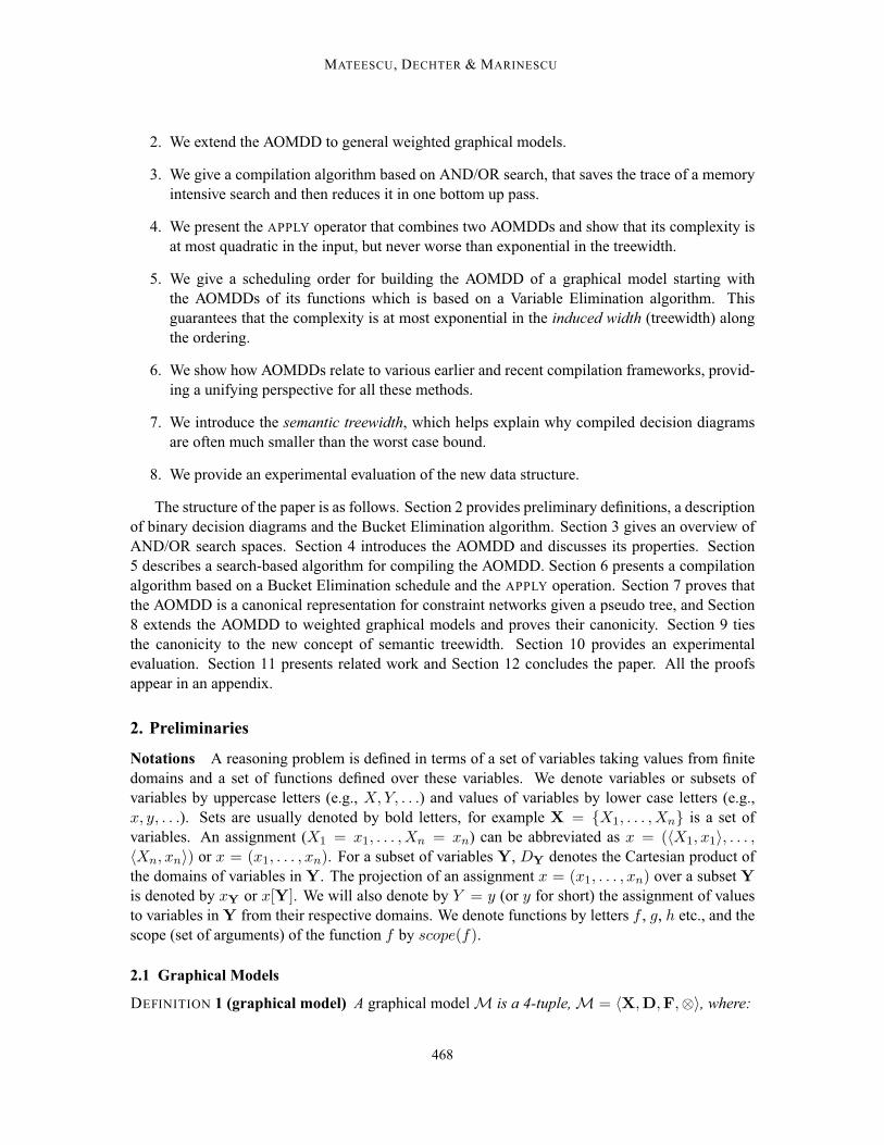
Example 7 Let’s look at the impact of caching on the size of the search space by examining a largerexample. Figure 7(a) shows a graphical model with binary variables and Figure 7(b) a pseudo treethat drives the AND/OR search. The context of each node is given in square brackets. The contextminimal graph is given in Figure 7(c). Note that it is far smaller than the AND/OR search tree,which has 28 = 256 AND nodes at the level of M alone (because M is at depth 8 in the pseudo tree).The shaded rectangles show the size of each cache table, equal to the number of OR nodes thatappear in each one. A cache entry is useful whenever there are more than one incoming edges intothe OR node. Incidentally, the caches that are not useful (namely OR nodes with only one incomingarc), are called dead caches (Darwiche, 2001), and can be determined based only on the pseudo
478
AND/OR MULTI-VALUED DECISION DIAGRAMS (AOMDDS) FOR GRAPHICAL MODELS
tree inspection, therefore a cache table need not be allocated for them. The context minimal graphcan also explain the execution of BE along the same pseudo tree (or, equivalently, along its depthfirst traversal order). The buckets are the shaded rectangles, and the processing is done bottom up.The number of possible assignments to each bucket equals the number of AND nodes that appearin it. The message scope is identical to the context of the bucket variable, and the message itself isidentical to the corresponding cache table. For more details on the relationship between AND/ORsearch and BE see the work of Mateescu and Dechter (2005).
3.3 Weighted AND/OR Graphs
In the previous subsections we described the structure of the AND/OR trees and graphs. In orderto use them to solve a reasoning task, we need to define a way of using the input function valuesduring the traversal of an AND/OR graph. This is realized by placing weights (or costs) on theOR-to-AND arcs, dictated by the function values. Only the functions that are relevant contribute toan OR-to-AND arc weight, and this is captured by the buckets relative to the pseudo tree:
DEFINITION 17 (buckets relative to a pseudo tree) Given a graphical modelM = 〈X,D,F,⊗〉and a pseudo tree T , the bucket of Xi relative to T , denoted BT (Xi), is the set of functions whosescopes contain Xi and are included in pathT (Xi), which is the set of variables from the root to Xi
in T . Namely,
BT (Xi) = {f ∈ F|Xi ∈ scope(f), scope(f) ⊆ pathT (Xi)}.
A function belongs to the bucket of a variable Xi iff its scope has just been fully instantiatedwhen Xi was assigned. Combining the values of all functions in the bucket, for the current assign-ment, gives the weight of the OR-to-AND arc:
DEFINITION 18 (OR-to-AND weights) Given an AND/OR graph of a graphical model M, theweight w(n,m)(Xi, xi) of arc (n, m) where Xi labels n and xi labels m, is the combination ofall the functions in BT (Xi) assigned by values along the current path to the AND node m, πm.Formally, w(n,m)(Xi, xi) = ⊗f∈BT (Xi)f(asgn(πm)[scope(f)]).
DEFINITION 19 (weight of a solution tree) Given a weighted AND/OR graph of a graphical modelM, and given a solution tree t having the OR-to-AND set of arcs arcs(t), the weight of t is definedby w(t) = ⊗e∈arcs(t)w(e).
Example 8 We start with the more straightforward case of constraint networks. Since functionsonly take values 0 or 1, and the combination is by product (join of relations), it follows that any OR-to-AND arc can only have a weight of 0 or 1. An example is given in Figure 8. Figure 8(a) showsa constraint graph, 8(b) a pseudo tree for it, and 8(c) the four relations that define the constraintproblem. Figure 8(d) shows the AND/OR tree that can be traversed by a depth first search algorithmthat only checks the consistency of the input functions (i.e., no constraint propagation is used).Similar to the OBDD representation, the OR-to-AND arcs with a weight of 0 are denoted by dottedlines, and the tree is not unfolded below them, since it will not contain any solution. The arcs witha weight of 1 are drawn with solid lines.
479

MATEESCU, DECHTER & MARINESCU
A
E
C
B
F
D
(a) Constraint graph
A
D
B
EC
F
(b) Pseudo tree
01111011110110011110001011001000
RABCCBA
01111011110100011110101001001000
RABEEBA
01111011110110011110101011000000
RAEFFEA
11111011010110010110101011001000
RBCDDCB
(c) Relations
A
0
B
0
E
F
0 1
0 1
C
D D
0 1 0 1
0 1
� � � � � �
�
1
E
F F
0 1 0 1
0 1
C
D
0 1
0 1
1
B
0
E
F
0 1
0 1
C
D D
0 1 0 1
0 1
1
E
F
0 1
0 1
C
D
0 1
0 1
� � � � � �
�
� � � � � � � � � �
� � �� � � �� � � �� � �
� � � �
� �
(d) AND/OR tree
Figure 8: AND/OR search tree for constraint networks
Example 9 Figure 9 shows a weighted AND/OR tree for a belief network. Figure 9(a) shows thedirected acyclic graph, and the dotted arc BC added by moralization. Figure 9(b) shows the pseudotree, and 9(c) shows the conditional probability tables. Figure 9(d) shows the weighted AND/ORtree.
As we did for constraint networks, we can move from weighted AND/OR search trees toweighted AND/OR search graphs by merging unifiable nodes. In this case the arc labels should bealso considered when determining unifiable subgraphs. This can yield context-minimal weightedAND/OR search graphs and minimal weighted AND/OR search graphs.
4. AND/OR Multi-Valued Decision Diagrams (AOMDDs)
In this section we begin describing the contributions of this paper. The context minimal AND/ORgraph (Definition 16) offers an effective way of identifying some unifiable nodes during the execu-tion of the search algorithm. Namely, context unifiable nodes are discovered based only on theirpaths from the root, without actually solving their corresponding subproblems. However, merg-ing based on context is not complete, which means that there may still exist unifiable nodes inthe search graph that do not have identical contexts. Moreover, some of the nodes in the context
480

AND/OR MULTI-VALUED DECISION DIAGRAMS (AOMDDS) FOR GRAPHICAL MODELS
A
D
B C
E
(a) Belief network
A
D
B
CE
(b) Pseudo tree
.2
.7
.5
.4
E=0
.811
.301
.510
.600
E=1BA
.1
.4
B=0
.91
.60
B=1A
.7
.2
C=0
.31
.80
C=1A
.4
.6
P(A)
1
0
A
.5
.3
.1
.2
D=0
.511
.701
.910
.800
D=1CB
P(E | A,B)P(D | B,C)
P(B | A) P(C | A)P(A)
(c) CPTs
0
A
B
0
E C
0
D
0 1
1
D
0 1
0 1
1
E C
0
D
0 1
1
D
0 1
0 1
1
B
0
E C
0
D
0 1
1
D
0 1
0 1
1
E C
0
D
0 1
1
D
0 1
0 1
.7.8 .9 .5 .7.8 .9 .5
.4 .5 .7 .2.2 .8 .2 .8 .7 .3 .7 .3
.4 .6 .1 .9
.6 .4
.6 .5 .3 .8
.2 .1 .3 .5 .2 .1 .3 .5
(d) Weighted AND/OR tree
Figure 9: Weighted AND/OR search tree for belief networks
minimal AND/OR graph may be redundant, for example when the set of solutions rooted at vari-able Xi is not dependant on the specific value assigned to Xi (this situation is not detectable basedon context). This is sometimes termed as “interchangeable values” or “symmetrical values”. Asoverviewed earlier, Dechter and Mateescu (2007, 2004a) defined the complete minimal AND/ORgraph which is an AND/OR graph whose unifiable nodes are all merged, and Dechter and Mateescu(2007) also proved the canonicity for non-weighted graphical models.In this paper we propose to augment the minimal AND/OR search graph with removing re-
dundant variables as is common in OBDD representation as well as adopt notational conventionscommon in this community. This yields a data structure that we call AND/OR BDD, that exploitsdecomposition by using AND nodes. We present the extension over multi-valued variables yieldingAND/OR MDD or AOMDD and define them for general weighted graphical models. Subsequentlywe present two algorithms for compiling the canonical AOMDD of a graphical model: the first issearch-based, and uses the memory intensive AND/OR graph search to generate the context minimalAND/OR graph, and then reduces it bottom up by applying reduction rules; the second is inference-based, and uses a Bucket Elimination schedule to combine the AOMDDs of initial functions byAPPLY operations (similar to the apply for OBDDs). As we will show, both approaches have thesame worst case complexity as the AND/OR graph search with context based caching, and also thesame complexity as Bucket Elimination, namely time and space exponential in the treewidth of theproblem, O(n kw∗). The benefit of each of these generation schemes will be discussed.
481
MATEESCU, DECHTER & MARINESCU
A
(a) OBDD
1 2 k
A
…(b) MDD
Figure 10: Decision diagram nodes (OR)
A
… …(a) AOBDD
A
… … ……1 2 k
(b) AOMDD
Figure 11: Decision diagram nodes (AND/OR)
4.1 From AND/OR Search Graphs to Decision Diagrams
An AND/OR search graph G of a graphical model M = 〈X,D,F,⊗〉 represents the set of allpossible assignments to the problem variables (all solutions and their costs). In this sense, G canbe viewed as representing the function f = ⊗fi∈Ffi that defines the universal equivalent graphicalmodel u(M) (Definition 2). For each full assignment x = (x1, . . . , xn), if x is a solution expressedby the tree tx, then f(x) = w(tx) = ⊗e∈arcs(tx)w(e) (Definition 19); otherwise f(x) = 0 (theassignment is inconsistent). The solution tree tx of a consistent assignment x can be read from Gin linear time by following the assignments from the root. If x is inconsistent, then a dead-end isencountered in G when attempting to read the solution tree tx, and f(x) = 0. Therefore, G can beviewed as a decision diagram that determines the values of f for every complete assignment x.We will now see how we can process an AND/OR search graph by reduction rules similar to
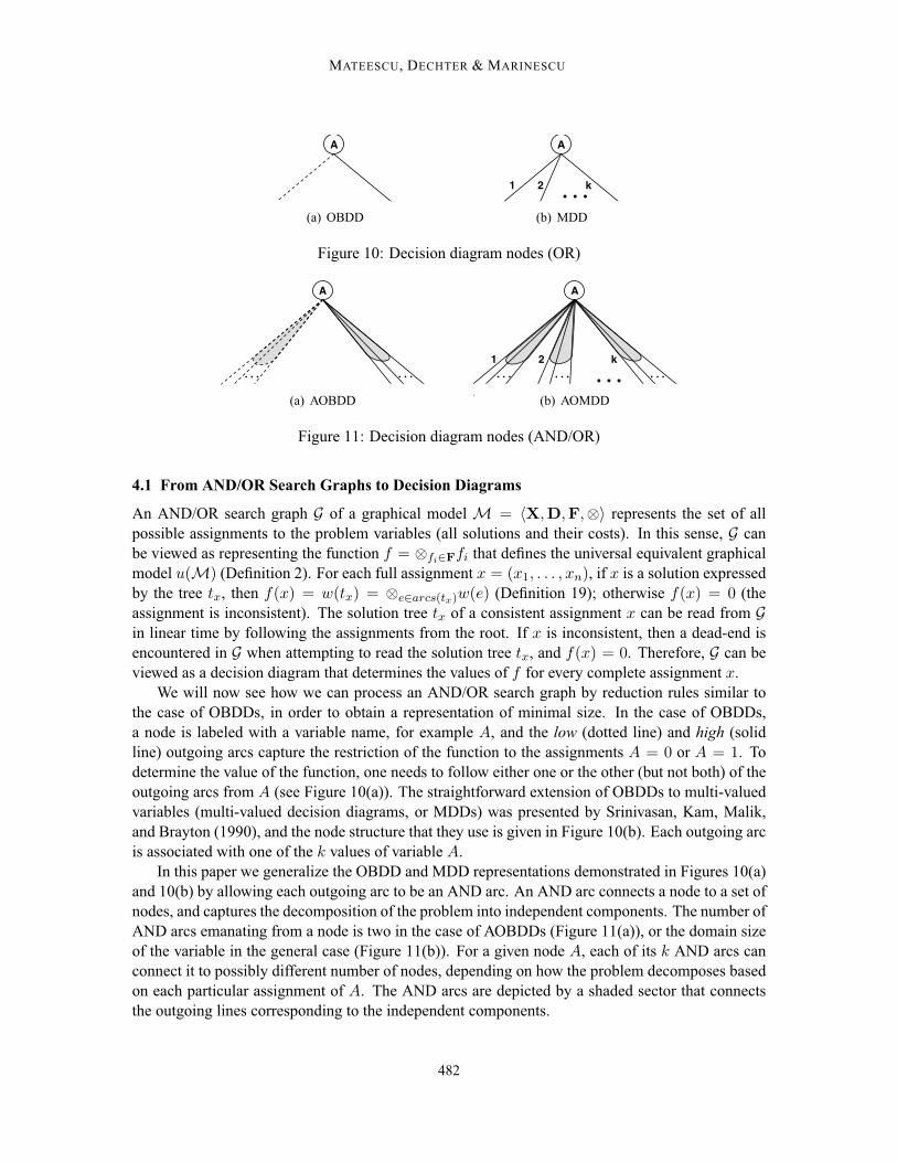
the case of OBDDs, in order to obtain a representation of minimal size. In the case of OBDDs,a node is labeled with a variable name, for example A, and the low (dotted line) and high (solidline) outgoing arcs capture the restriction of the function to the assignments A = 0 or A = 1. Todetermine the value of the function, one needs to follow either one or the other (but not both) of theoutgoing arcs from A (see Figure 10(a)). The straightforward extension of OBDDs to multi-valuedvariables (multi-valued decision diagrams, or MDDs) was presented by Srinivasan, Kam, Malik,and Brayton (1990), and the node structure that they use is given in Figure 10(b). Each outgoing arcis associated with one of the k values of variable A.In this paper we generalize the OBDD and MDD representations demonstrated in Figures 10(a)
and 10(b) by allowing each outgoing arc to be an AND arc. An AND arc connects a node to a set ofnodes, and captures the decomposition of the problem into independent components. The number ofAND arcs emanating from a node is two in the case of AOBDDs (Figure 11(a)), or the domain sizeof the variable in the general case (Figure 11(b)). For a given node A, each of its k AND arcs canconnect it to possibly different number of nodes, depending on how the problem decomposes basedon each particular assignment of A. The AND arcs are depicted by a shaded sector that connectsthe outgoing lines corresponding to the independent components.
482

AND/OR MULTI-VALUED DECISION DIAGRAMS (AOMDDS) FOR GRAPHICAL MODELS
… … ……
A
1 2 k…
(a) Nonterminal meta-node
0
(b) Terminal meta-node 0
1
(c) Terminal meta-node 1
Figure 12: Meta-nodes
We define the AND/OR Decision Diagram representation based on AND/OR search graphs. Wefind that it is useful to maintain the semantics of Figure 11 especially when we need to express theredundancy of nodes, and therefore we introduce the meta-node data structure, which defines smallportions of any AND/OR graph, based on an OR node and its AND children:
DEFINITION 20 (meta-node) A meta-node u in an AND/OR search graph can be either: (1) aterminal node labeled with 0 or 1, or (2) a nonterminal node, that consists of an OR node labeledX (therefore var(u) = X) and its k AND children labeled x1, . . . , xk that correspond to the valueassignments of X . Each AND node labeled xi stores a list of pointers to child meta-nodes, denotedby u.childreni. In the case of weighted graphical models, the AND node xi also stores the OR-to-AND arc weight w(X, xi).
The rectangle in Figure 12(a) is a meta-node for variable A, that has a domain of size k. Notethat this is very similar to Figure 11, with the small difference that the information about the value ofA that corresponds to each outgoing AND arc is now stored in the AND nodes of the meta-node. Weare not showing the weights in that figure. A larger example of an AND/OR graph with meta-nodesappears later in Figure 16.The terminal meta-nodes play the role of the terminal nodes in OBDDs. The terminal meta-
node 0, shown in Figure 12(b), indicates inconsistent assignments, while the terminal meta-node 1,shown in figure 12(c) indicates consistent ones.Any AND/OR search graph can now be viewed as a diagram of meta-nodes, simply by grouping
OR nodes with their AND children, and adding the terminal meta-nodes appropriately.Once we have defined the meta-nodes, it is easier to see when a variable is redundant with re-
spect to the outcome of the function based on the current partial assignment. A variable is redundantif any of its assignments leads to the same set of solutions.
DEFINITION 21 (redundant meta-node) Given a weighted AND/OR search graph G representedwith meta-nodes, a meta-node u with var(u) = X and |D(X)| = k is redundant iff:(a) u.children1 = . . . = u.childrenk and(b) w(X, x1) = . . . = w(X, xk).
An AND/OR graph G, that contains a redundant meta-node u, can be transformed into an equiv-alent graph G′ by replacing any incoming arc into u with its common list of children u.children1,absorbing the common weight w(X, x1) by combination into the weight of the parent meta-nodecorresponding to the incoming arc, and then removing u and its outgoing arcs from G. Thevalue X = x1 is picked here arbitrarily, because they are all isomorphic. If u is the root of the
483

MATEESCU, DECHTER & MARINESCU
Procedure RedundancyReductioninput : AND/OR graph G; redundant meta-node u, with var(u) = X; List of meta-node parents of u,
denoted by Parents(u).output : Reduced AND/OR graph G after the elimination of u.if Parents(u) is empty then1
return independent AND/OR graphs rooted by meta-nodes in u.children1, and constant w(X, x1)2
forall v ∈ Parents(u) (assume var(v) == Y ) do3forall i ∈ {1, . . . , |D(Y )|} do4
if u ∈ v.childreni then5v.childreni ← v.childreni \ {u}6v.childreni ← v.childreni ∪ u.children17w(Y, yi) ← w(Y, yi) ⊗ w(X, x1)8
remove u9
return reduced AND/OR graph G10
Procedure IsomorphismReductioninput : AND/OR graph G; isomorphic meta-nodes u and v; List of meta-node parents of u, denoted by
Parents(u).output : Reduced AND/OR graph G after the merging of u and v.forall p ∈ Parents(u) do1
if u ∈ p.childreni then2p.childreni ← p.childreni \ {u}3p.childreni ← p.childreni ∪ {v}4
remove u5
return reduced AND/OR graph G6
graph, then the common weight w(X, x1) has to be stored separately as a constant. ProcedureRedundancyReduction formalizes the redundancy elimination.
DEFINITION 22 (isomorphic meta-nodes) Given a weighted AND/OR search graph G representedwith meta-nodes, two meta-nodes u and v having var(u) = var(v) = X and |D(X)| = k areisomorphic iff:(a) u.childreni = v.childreni ∀i ∈ {1, . . . , k} and(b) wu(X, xi) = wv(X, xi) ∀i ∈ {1, . . . , k}, (where wu, wv are the weights of u and v).
Procedure IsomorphismReduction formalizes the process of merging isomorphic meta-nodes. Naturally, the AND/OR graph obtained by merging isomorphic meta-nodes is equivalent tothe original one. We can now define the AND/OR Multi-Valued Decision Diagram:
DEFINITION 23 (AOMDD) An AND/OR Multi-Valued Decision Diagram (AOMDD) is a weightedAND/OR search graph that is completely reduced by isomorphic merging and redundancy removal,namely:(1) it contains no isomorphic meta-nodes; and(2) it contains no redundant meta-nodes.
484

AND/OR MULTI-VALUED DECISION DIAGRAMS (AOMDDS) FOR GRAPHICAL MODELS
B
1 2 k…
c d y…
A
1 2 k…
z
(a) Fragment of an AOMDD
c d y…
A
1 2 k…
z
(b) After eliminating the B
meta-node
Figure 13: Redundancy reduction
C
1 2 k…
d e y…
A
1 2 k…
C
1 2 k…
B
1 2 k…
(a) Fragment of an AOMDD
C
1 2 k…
d e y…
A
1 2 k…B
1 2 k…
(b) After merging the isomor-phic C meta-nodes
Figure 14: Isomorphism reduction
Example 10 Figure 13 shows an example of applying the redundancy reduction rule to a portionof an AOMDD. On the left side, in Figure 13(a), the meta-node of variable B is redundant (wedon’t show the weights of the OR-to-AND arcs, to avoid cluttering the figure). Any of the values{1, . . . , k} of B will lead to the same set of meta-nodes {c, d, . . . , y}, which are coupled in an ANDarc. Therefore, the meta-node of B can be eliminated. The result is shown in Figure 13(b), wherethe meta-nodes {c, d, . . . , y} and z are coupled in an AND arc outgoing from A = 1.In Figure 14 we show an example of applying the isomorphism reduction rule. In this case, the
meta-nodes labeled with C in Figure 14(a) are isomorphic (again, we omit the weights). The resultof merging them is shown in Figure 14(b).
Examples of AOMDDs appear in Figures 16, 17 and 18. Note that if the weight on an OR-to-AND arc is zero, then the descendant is the terminal meta-node 0. Namely, the current path is adead-end, cannot be extended to a solution, and is therefore linked directly to 0.
5. Using AND/OR Search to Generate AOMDDs
In Section 4.1 we described how we can transform an AND/OR graph into an AOMDD by applyingreduction rules. In Section 5.1 we describe the explicit algorithm that takes as input a graphi-
485
MATEESCU, DECHTER & MARINESCU
cal model, performs AND/OR search with context-based caching to obtain the context minimalAND/OR graph, and in Section 5.2 we give the procedure that applies the reduction rules bottomup to obtain the AOMDD.
5.1 Algorithm AND/OR-SEARCH-AOMDD
Algorithm 1, called AND/OR-SEARCH-AOMDD, compiles a graphical model into an AOMDD.Amemory intensive (with context-based caching) AND/OR search is used to create the context min-imal AND/OR graph (see Definition 16). The input to AND/OR-SEARCH-AOMDD is a graphicalmodelM and a pseudo tree T , that also defines the OR-context of each variable.Each variable Xi has an associated cache table, whose scope is the context of Xi in T . This
ensures that the trace of the search is the context minimal AND/OR graph. A list denoted by LXi
(see line 35), is used for each variable Xi to save pointers to meta-nodes labeled with Xi. Theselists are used by the procedure that performs the bottom up reduction, per layers of the AND/ORgraph (one layer contains all the nodes labeled with one given variable). The fringe of the searchis maintained on a stack called OPEN. The current node (either OR or AND node) is denoted byn, its parent by p, and the current path by πn. The children of the current node are denoted bysuccessors(n). For each node n, the Boolean attribute consistent(n) indicates if the current pathcan be extended to a solution. This information is useful for pruning the search space.The algorithm is based on two mutually recursive steps: Forward (beginning at line 5) and
Backtrack (beginning at line 29), which call each other (or themselves) until the search terminates.In the forward phase, the AND/OR graph is expanded top down. The two types of nodes, AND andOR, are treated differently according to their semantics.Before an OR node is expanded, the cache table of its variable is checked (line 8). If the entry
is not null, a link is created to the already existing OR node that roots the graph equivalent to thecurrent subproblem. Otherwise, the OR node is expanded by generating its AND descendants. TheOR-to-AND weight (see Definition 18) is computed in line 13. Each value xi of Xi is checked forconsistency (line 14). The least expensive check is to verify that the OR-to-ANDweight is non-zero.However, the deterministic (inconsistent) assignments inM can be extracted to form a constraintnetwork. Any level of constraint propagation can be performed in this step (e.g., look ahead, arcconsistency, path consistency, i-consistency etc.). The computational overhead can increase, in thehope of pruning the search space more aggressively. We should note that constraint propagation isnot crucial for the algorithm, and the complexity guarantees are maintained even if only the simpleweight check is performed. The consistent AND nodes are added to the list of successors of n (line16), while the inconsistent ones are linked to the terminal 0 meta-node (line 19).An AND node n labeled with 〈Xi, xi〉 is expanded (line 20) based on the structure of the pseudo
tree. If Xi is a leaf in T , then n is linked to the terminal 1 meta-node (line 22). Otherwise, an ORnode is created for each child of Xi in T (line 24).The forward step continues as long as the current node is not a dead-end and still has unevaluated
successors. The backtrack phase is triggered when a node has an empty set of successors (line 29).Note that, as each successor is processed, it is removed from the set of successors in line 42. Whenthe backtrack reaches the root (line 32), the search is complete, the context minimal AND/OR graphis generated, and the Procedure BOTTOMUPREDUCTION is called.When the backtrack step processes an OR node (line 31), it saves a pointer to it in cache, and
also adds a pointer to the corresponding meta-node to the list LXi . The consistent attribute of
486

AND/OR MULTI-VALUED DECISION DIAGRAMS (AOMDDS) FOR GRAPHICAL MODELS
Algorithm 1: AND/OR SEARCH - AOMDDinput :M = 〈X,D,F〉; pseudo tree T rooted atX1; parents pai (OR-context) for every variableXi.output : AOMDD ofM.forallXi ∈ X do1
Initialize context-based cache table CacheXi(pai) with null entries2
Create new OR node t, labeled withXi; consistent(t) ← true; push t on top of OPEN3while OPEN �= φ do4
n ← top(OPEN); remove n from OPEN // Forward5successors(n) ← φ6if n is an OR node labeled withXi then // OR-expand7
if CacheXi(asgn(πn)[pai]) �= null then8
Connect parent of n to CacheXi(asgn(πn)[pai]) // Use the cached pointer9
else10forall xi ∈ Di do11
Create new AND node t, labeled with 〈Xi, xi〉12w(X, xi) ← ⊗
f∈BT (Xi)f(asgn(πn)[pai])13
if 〈Xi, xi〉 is consistent with πn then // Constraint Propagation14consistent(t) ← true15add t to successors(n)16
else17consistent(t) ← false18make terminal 0 the only child of t19
if n is an AND node labeled with 〈Xi, xi〉 then // AND-expand20if childrenT (Xi) == φ then21
make terminal 1 the only child of n22else23
forall Y ∈ childrenT (Xi) do24Create new OR node t, labeled with Y25consistent(t) ← false26add t to successors(n)27
Add successors(n) to top of OPEN28while successors(n) == φ do // Backtrack29
let p be the parent of n30if n is an OR node labeled withXi then31
ifXi == X1 then // Search is complete32Call BottomUpReduction procedure // begin reduction to AOMDD33
Cache(asgn(πn)[pai]) ← n // Save in cache34Add meta-node of n to the list LXi35consistent(p) ← consistent(p) ∧ consistent(n)36if consistent(p) == false then // Check if p is dead-end37
remove successors(p) from OPEN38successors(p) ← φ39
if n is an AND node labeled with 〈Xi, xi〉 then40consistent(p) ← consistent(p) ∨ consistent(n);41
remove n from successors(p)42n ← p43
487

MATEESCU, DECHTER & MARINESCU
Procedure BottomUpReductioninput : A graphical modelM = 〈X,D,F〉; a pseudo tree T of the primal graph, rooted atX1; Context
minimal AND/OR graph, and lists LXi of meta-nodes for each levelXi.output : AOMDD ofM.Let d = {X1, . . . , Xn} be the depth first traversal ordering of T1for i ← n down to 1 do2
LetH be a hash table, initially empty3forall meta-nodes n in LXi do4
ifH(Xi, n.children1, . . . , n.childrenki, wn(Xi, x1), . . . , w
n(Xki, xki
)) returns a meta-node5p then
merge n with p in the AND/OR graph6
else if n is redundant then7eliminate n from the AND/OR graph8combine its weight with that of the parent9
else10hash n into the table H:11H(Xi, n.children1, . . . , n.childrenki
, wn(Xi, x1), . . . , wn(Xki
, xki)) ← n12
return reduced AND/OR graph13
the AND parent p is updated by conjunction with consistent(n). If the AND parent p becomesinconsistent, it is not necessary to check its remaining OR successors (line 38). When the backtrackstep processes an AND node (line 40), the consistent attribute of the OR parent p is updated bydisjunction with consistent(n).The AND/OR search algorithm usually maintains a value for each node, corresponding to a task
that is solved. We did not include values in our description because an AOMDD is just an equivalentrepresentation of the original graphical modelM. Any task overM can be solved by a traversalof the AOMDD. It is however up to the user to include more information in the meta-nodes (e.g.,number of solutions for a subproblem).
5.2 Reducing the Context Minimal AND/OR Graph to an AOMDD
Procedure BottomUpReduction processes the variables bottom up relative to the pseudo tree T .We use the depth first traversal ordering of T (line 1), but any other bottom up ordering is as good.The outer for loop (starting at line 2) goes through each level of the context minimal AND/OR graph(where a level contains all the OR and AND nodes labeled with the same variable, in other words itcontains all the meta-nodes of that variable). For efficiency, and to ensure the complexity guaranteesthat we will prove, a hash table, initially empty, is used for each level. The inner for loop (starting atline 4) goes through all the metanodes of a level, that are also saved (or pointers to them are saved)in the list LXi . For each new meta-node n in the list LXi , in line 5 the hash table H is checked toverify if a node isomorphic with n already exists. If the hash tableH already contains a node p cor-responding to the hash key (Xi, n.children1, . . . , n.childrenki
, wn(Xi, x1), . . . , wn(Xki
, xki)),
then p and n are isomorphic and should be merged. Otherwise, if the new meta-node n is redundant,then it is eliminated from the AND/OR graph. If none of the previous two conditions is met, thenthe new meta-node n is hashed into table H .
488

AND/OR MULTI-VALUED DECISION DIAGRAMS (AOMDDS) FOR GRAPHICAL MODELS
D
C B F
AE
G
H
A
B
C F
D E G H
(a) (b)
Figure 15: (a) Constraint graph for C = {C1, . . . , C9}, where C1 = F ∨ H , C2 = A ∨ ¬H ,C3 = A⊕B⊕G, C4 = F ∨G, C5 = B ∨F , C6 = A∨E, C7 = C ∨E, C8 = C ⊕D,C9 = B ∨ C; (b) Pseudo tree (bucket tree) for ordering d = (A, B, C, D, E, F, G, H)
Proposition 1 The output of Procedure BottomUpReduction is the AOMDD ofM along thepseudo tree T , namely the resulting AND/OR graph is completely reduced.
Note that we explicated Procedure BottomUpReduction separately only for clarity. In prac-tice, it can actually be included in Algorithm AND/OR-SEARCH-AOMDD, and the reduction rulescan be applied whenever the search backtracks. We can maintain a hash table for each variable, dur-ing the AND/OR search, to store pointers to meta-nodes. When the search backtracks out of anOR node, it can already check the redundancy of that meta-node, and also look up in the hash tableto check for isomorphism. Therefore, the reduction of the AND/OR graph can be done during theAND/OR search, and the output will be the AOMDD ofM.From Theorem 3 and Proposition 1 we can conclude:
THEOREM 4 Given a graphical modelM and a pseudo tree T of its primal graph G, the AOMDDofM corresponding to T has size bounded by O(n kw∗
T(G)) and it can be computed by Algorithm
AND/OR-SEARCH-AOMDD in time O(n kw∗T
(G)), where w∗T (G) is the induced width of G over
the depth first traversal of T , and k bounds the domain size.
6. Using Bucket Elimination to Generate AOMDDs
In this section we propose to use a Bucket Elimination (BE) type algorithm to guide the compilationof a graphical model into an AOMDD. The idea is to express the graphical model functions asAOMDDs, and then combine them with APPLY operations based on a BE schedule. The APPLY isvery similar to that from OBDDs (Bryant, 1986), but it is adapted to AND/OR search graphs. Ittakes as input two functions represented as AOMDDs based on the same pseudo tree, and outputsthe combination of initial functions, also represented as an AOMDD based on the same pseudo tree.We will describe it in detail in Section 6.2.We will start with an example based on constraint networks. This is easier to understand because
the weights on the arcs are all 1 or 0, and therefore are depicted in the figures by solid and dashedlines, respectively.
Example 11 Consider the network defined byX = {A, B, . . . , H},DA = . . . = DH = {0, 1} andthe constraints (where⊕ denotes XOR):C1 = F∨H ,C2 = A∨¬H ,C3 = A⊕B⊕G,C4 = F∨G,
489
MATEESCU, DECHTER & MARINESCU
HG
ED
CF
B
A
F0 1
H0 1
0 1C1
A0 1
H0 1
0 1C2
A0 1
B0 1
G0 1
G0 1
B0 1
0 1C3
F0 1
G0 1
0 1C4
A0 1
E0 1
0 1C6
C0 1
E0 1
0 1C7
C0 1
D0 1
D0 1
0 1C8
B0 1
C0 1
0 1C9
B0 1
F0 1
0 1C5
m1
m3
m7
m6
m4 m2m 5
A0 1
F0 1
H0 1
F0 1
H0 1
0 1m1
A0 1
B0 1
G0 1
F0 1
B0 1
G0 1
0 1m2
A0 1
E0 1
C0 1
0 1m4
C0 1
D0 1
D0 1
0 1m5
A0 1
B0 1
F0 1
G0 1
H0 1
F0 1
G0 1
B0 1
F0 1
F0 1
H0 1
0 1m3
A0 1
B0 1
C0 1
C0 1
D0 1
E0 1
D0 1
B0 1
C0 1
C0 1
0 1m6
m7
A
F
H
A
B
F
G H
C
D
A
B
C
D E
A
B
C F
D E G H
A
B
F
G
C
E
A
Figure 16: Execution of BE with AOMDDs
A0 1
B0 1
C0 1
0
D0 1
1
F0 1
G0 1
H0 1
C0 1
D0 1
E0 1
F0 1
G0 1
B0 1
C0 1
F0 1
C0 1
F0 1
H0 1
(a)
D
C
B
F
A
E
G
H
1 0
B
CC C
D D D D D
E E
F F F
G G G G
H
(b)
Figure 17: (a) The final AOMDD; (b) The OBDD corresponding to d
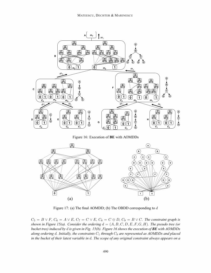
C5 = B ∨ F , C6 = A ∨ E, C7 = C ∨ E, C8 = C ⊕ D, C9 = B ∨ C. The constraint graph isshown in Figure 15(a). Consider the ordering d = (A, B, C, D, E, F, G, H). The pseudo tree (orbucket tree) induced by d is given in Fig. 15(b). Figure 16 shows the execution of BE with AOMDDsalong ordering d. Initially, the constraints C1 through C9 are represented as AOMDDs and placedin the bucket of their latest variable in d. The scope of any original constraint always appears on a
490

AND/OR MULTI-VALUED DECISION DIAGRAMS (AOMDDS) FOR GRAPHICAL MODELS
Algorithm 2: BE-AOMDDinput : Graphical modelM = 〈X,D,F〉, whereX = {X1, . . . , Xn}, F = {f1, . . . , fr} ; order
d = (X1, . . . , Xn)output : AOMDD representing ⊗i∈Ffi
T = GeneratePseudoTree(G, d);1for i ← 1 to r do // place functions in buckets2
place Gaomddfi
in the bucket of its latest variable in d3
for i ← n down to 1 do // process buckets4message(Xi) ← Gaomdd
1 // initialize with AOMDD of 1 ;5while bucket(Xi) �= φ do // combine AOMDDs in bucket of Xi6
pick Gaomddf from bucket(Xi);7
bucket(Xi) ← bucket(Xi) \ {Gaomddf };8
message(Xi) ← APPLY(message(Xi),Gaomddf )9
addmessage(Xi) to the bucket of the parent ofXi in T10
returnmessage(X1)11
path from root to a leaf in the pseudo tree. Therefore, each original constraint is represented by anAOMDD based on a chain (i.e., there is no branching into independent components at any point).The chain is just the scope of the constraint, ordered according to d. For bi-valued variables, theoriginal constraints are represented by OBDDs, for multiple-valued variables they are MDDs. Notethat we depict meta-nodes: one OR node and its two AND children, that appear inside each graynode. The dotted edge corresponds to the 0 value (the low edge in OBDDs), the solid edge to the1 value (the high edge). We have some redundancy in our notation, keeping both AND value nodesand arc-types (dotted arcs from “0” and solid arcs from “1”).The BE scheduling is used to process the buckets in reverse order of d. A bucket is processed
by joining all the AOMDDs inside it, using the APPLY operator. However, the step of eliminationof the bucket variable is omitted because we want to generate the full AOMDD. In our example,the messages m1 = C1 �� C2 and m2 = C3 �� C4 are still based on chains, therefore they areOBDDs. Note that they contain the variables H and G, which have not been eliminated. However,the message m3 = C5 �� m1 �� m2 is not an OBDD anymore. We can see that it follows thestructure of the pseudo tree, where F has two children, G andH . Some of the nodes correspondingto F have two outgoing edges for value 1.The processing continues in the same manner. The final output of the algorithm, which coincides
with m7, is shown in Figure 17(a). The OBDD based on the same ordering d is shown in Fig.17(b). Notice that the AOMDD has 18 nonterminal nodes and 47 edges, while the OBDD has 27nonterminal nodes and 54 edges.
6.1 Algorithm BE-AOMDD
Algorithm 2, called BE-AOMDD, creates the AOMDD of a graphical model by using a BE sched-ule for APPLY operations. Given an order d of the variables, first a pseudo tree is created based onthe primal graph. Each initial function fi is then represented as an AOMDD, denoted by Gaomdd
fi,
and placed in its bucket. To obtain the AOMDD of a function, the scope of the function is orderedaccording to d, a search tree (based on a chain) that represents fi is generated, and then reducedby Procedure BottomUpReduction. The algorithm proceeds exactly like BE, with the only dif-ference that the combination of functions is realized by the APPLY algorithm, and variables are not
491

MATEESCU, DECHTER & MARINESCU
eliminated but carried over to the destination bucket. The messages between buckets are initializedwith the dummy AOMDD of 1, denoted by Gaomdd
1, which is neutral for combination.
In order to create the compilation of a graphical model based on AND/OR graphs, it is necessaryto traverse the AND/OR graph top down and bottom up. This is similar to the inward and outwardmessage passing in a tree decomposition. Note that BE-AOMDD describes the bottom up traversalexplicitly, while the top down phase is actually performed by the APPLY operation. When twoAOMDDs are combined, after the top chain portion of their pseudo tree is processed, the remainingindependent branches are attached only if they participate in the newly restricted set of solutions.This amounts to an exchange of information between the independent branches, which is equivalentto the top down phase.
6.2 The AOMDD APPLY Operation
We will now describe how to combine two AOMDDs. The APPLY operator takes as input twoAOMDDs representing functions f1 and f2 and returns an AOMDD representing f1 ⊗ f2.In OBDDs the apply operator combines two input diagrams based on the same variable ordering.
Likewise, in order to combine two AOMDDs we assume that their pseudo trees are identical. Thiscondition is satisfied by any two AOMDDs in the same bucket of BE-AOMDD. However, wepresent here a version of APPLY that is more general, by relaxing the previous condition fromidentical to compatible pseudo trees. Namely, there should be a pseudo tree in which both can beembedded. In general, a pseudo tree induces a strict partial order between the variables where aparent node always precedes its child nodes.
DEFINITION 24 (compatible pseudo trees) A strict partial order d1 = (X, <1) over a set X isconsistent with a strict partial order d2 = (Y, <2) over a set Y, if for all x1, x2 ∈ X ∩ Y, ifx1 <2 x2 then x1 <1 x2. Two partial orders d1 and d2 are compatible iff there exists a partialorder d that is consistent with both. Two pseudo trees are compatible iff the partial orders inducedvia the parent-child relationship, are compatible.
For simplicity, we focus on a more restricted notion of compatibility, which is sufficient whenusing a BE like schedule for the APPLY operator to combine the input AOMDDs (as described inSection 6). The APPLY algorithm that we will present can be extended to the more general notionof compatibility.
DEFINITION 25 (strictly compatible pseudo trees) A pseudo tree T1 having the set of nodes X1
can be embedded in a pseudo tree T having the set of nodesX ifX1 ⊆ X and T1 can be obtainedfrom T by deleting each node in X \ X1 and connecting its parent to each of its descendents. Twopseudo trees T1 and T2 are strictly compatible if there exists T such that both T1 and T2 can beembedded in T .
Algorithm APPLY (algorithm 3) takes as input one node from Gaomddf and a list of nodes from
Gaomddg . Initially, the node from Gaomdd
f is its root node, and the list of nodes from Gaomddg is in fact
also made of just one node, which is its root. We will sometimes identify an AOMDD by its rootnode. The pseudo trees Tf and Tg are strictly compatible, having a target pseudo tree T .The list of nodes from Gaomdd
g always has a special property: there is no node in it that can be theancestor in T of another (we refer to the variable of the meta-node). Therefore, the list z1, . . . , zm
492

AND/OR MULTI-VALUED DECISION DIAGRAMS (AOMDDS) FOR GRAPHICAL MODELS
Algorithm 3: APPLY(v1; z1, . . . , zm)input : AOMDDs Gaomdd
f with nodes vi and Gaomddg with nodes zj , based on strictly compatible pseudo
trees Tf , Tg that can be embedded in T .var(v1) is an ancestor of all var(z1), . . . , var(zm) in T .var(zi) and var(zj) are not in ancestor-descendant relation in T , ∀i �= j.
output : v1 ⊗ (z1 ∧ . . . ∧ zm), based on T .ifH1(v1, z1, . . . , zm) �= null then returnH1(v1, z1, . . . , zm); // is in cache1if (any of v1, z1, . . . , zm is 0) then return 02if (v1 = 1) then return 13if (m = 0) then return v1 // nothing to combine4create new nonterminal meta-node u5var(u) ← var(v1) (call itXi, with domainDi = {x1, . . . , xki
} )6for j ← 1 to ki do7
u.childrenj ← φ // children of the j-th AND node of u8wu(Xi, xj) ← wv1(Xi, xj) // assign weight from v19if ( (m = 1) and (var(v1) = var(z1) = Xi) ) then10
temp Children ← z1.childrenj11wu(Xi, xj) ← wv1(Xi, xj) ⊗ wz1(Xi, xj) // combine input weights12
else13temp Children ← {z1, . . . , zm}14
group nodes from v1.childrenj ∪ temp Children in several {v1; z1, . . . , zr}15for each {v1; z1, . . . , zr} do16
y ← APPLY(v1; z1, . . . , zr)17if (y = 0) then18
u.childrenj ← 0; break19
else20u.childrenj ← u.childrenj ∪ {y}21
if (u.children1 = . . . = u.childrenki) and (wu(Xi, x1) = . . . = wu(Xi, xki
)) then22promote wu(Xi, x1) to parent23return u.children1 // redundancy24
if (H2(Xi, u.children1, . . . , u.childrenki, wu(Xi, x1), . . . , w
u(Xki, xki
)) �= null) then25returnH2(Xi, u.children1, . . . , u.childrenki
, wu(Xi, x1), . . . , wu(Xki
, xki))26
// isomorphism
LetH1(v1, z1, . . . , zm) = u // add u to H127LetH2(Xi, u.children1, . . . , u.childrenki
, wu(Xi, x1), . . . , wu(Xki
, xki)) = u // add u to H228
return u29
from g expresses a decomposition with respect to T , so all those nodes appear on different branches.We will employ the usual techniques from OBDDs to make the operation efficient. First, if one ofthe arguments is 0, then we can safely return 0. Second, a hash table H1 is used to store the nodesthat have already been processed, based on the nodes (v1, z1, . . . , zr). Therefore, we never needto make multiple recursive calls on the same arguments. Third, a hash table H2 is used to detectisomorphic nodes. This is typically split in separate tables for each variable. If at the end of therecursion, before returning a value, we discover that a meta-node with the same variable, the samechildren and the same weights has already been created, then we don’t need to store it and we simplyreturn the existing node. And fourth, if at the end of the recursion we discover that we created aredundant node (all the children are the same and all the weights are the same), then we don’t storeit, and return instead one of its identical lists of children, and promote the common weight.
493
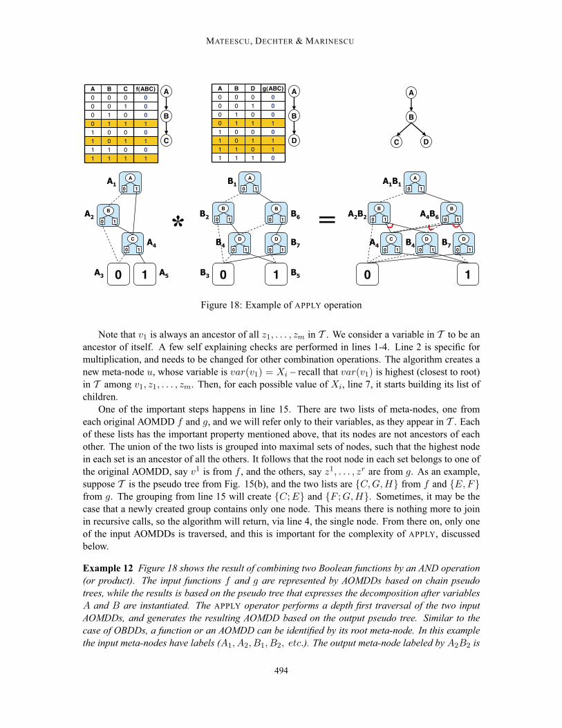
MATEESCU, DECHTER & MARINESCU
0
A
0 1
B
0 1
1
C
0 1
��
��
��
��
��
A
B
C
11110011110100011110001001000000
f(ABC)CBA A
B
D
01111011110100011110001001000000
g(ABC)DBA
0
A
0 1
B
0 1
1
D
0 1
D
0 1
B
0 1
�
�
�
�
�
�
A
B
DC
* =
A
0 1���
B
0 1���
0
C
0 1��
D
0 1�
1
B
0 1��
D
0 1�
Figure 18: Example of APPLY operation
Note that v1 is always an ancestor of all z1, . . . , zm in T . We consider a variable in T to be anancestor of itself. A few self explaining checks are performed in lines 1-4. Line 2 is specific formultiplication, and needs to be changed for other combination operations. The algorithm creates anew meta-node u, whose variable is var(v1) = Xi – recall that var(v1) is highest (closest to root)in T among v1, z1, . . . , zm. Then, for each possible value of Xi, line 7, it starts building its list ofchildren.One of the important steps happens in line 15. There are two lists of meta-nodes, one from
each original AOMDD f and g, and we will refer only to their variables, as they appear in T . Eachof these lists has the important property mentioned above, that its nodes are not ancestors of eachother. The union of the two lists is grouped into maximal sets of nodes, such that the highest nodein each set is an ancestor of all the others. It follows that the root node in each set belongs to one ofthe original AOMDD, say v1 is from f , and the others, say z1, . . . , zr are from g. As an example,suppose T is the pseudo tree from Fig. 15(b), and the two lists are {C, G, H} from f and {E, F}from g. The grouping from line 15 will create {C; E} and {F ; G, H}. Sometimes, it may be thecase that a newly created group contains only one node. This means there is nothing more to joinin recursive calls, so the algorithm will return, via line 4, the single node. From there on, only oneof the input AOMDDs is traversed, and this is important for the complexity of APPLY, discussedbelow.
Example 12 Figure 18 shows the result of combining two Boolean functions by an AND operation(or product). The input functions f and g are represented by AOMDDs based on chain pseudotrees, while the results is based on the pseudo tree that expresses the decomposition after variablesA and B are instantiated. The APPLY operator performs a depth first traversal of the two inputAOMDDs, and generates the resulting AOMDD based on the output pseudo tree. Similar to thecase of OBDDs, a function or an AOMDD can be identified by its root meta-node. In this examplethe input meta-nodes have labels (A1, A2, B1, B2, etc.). The output meta-node labeled by A2B2 is
494

AND/OR MULTI-VALUED DECISION DIAGRAMS (AOMDDS) FOR GRAPHICAL MODELS
the root of a diagram that represents the function obtained by combining the functions rooted by A2
and B2.
6.3 Complexity of APPLY and BE-AOMDD
We now provide a characterization of the complexity of APPLY, based on different criteria. Thefollowing propositions are inspired by the results that govern OBDD apply complexity, but areadapted for pseudo tree orderings.An AOMDD along a pseudo tree can be regarded as a union of regular MDDs, each restricted
to a full path from root to a leaf in the pseudo tree. Let πT be such a path in T . Based on thedefinition of strictly compatible pseudo trees, πT has corresponding paths πTf
in Tf and πTg in Tg.The MDDs from f and g corresponding to πTf
and πTg can be combined using the regular MDDapply. This process can be repeated for every path πT . The resulting MDDs, one for each path in Tneed to be synchronized on their common parts (on the intersection of the paths). The algorithm weproposed does all this processing at once, in a depth first search traversal over the inputs. Based onour construction, we can give a first characterization of the complexity of AOMDD APPLY as beinggoverned by the complexity of MDD apply.
Proposition 2 Let π1, . . . , πl be the set of paths in T enumerated from left to right and let Gif and
Gig be the MDDs restricted to path πi, then the size of the output of AOMDD apply is bounded by∑i |G
if | · |G
ig| ≤ n · maxi|G
if | · |G
ig|. The time complexity is also bounded by
∑i |G
if | · |G
ig| ≤
n · maxi|Gif | · |G
ig|.
A second characterization of the complexity can be given, similar to the MDD case, in terms oftotal number of nodes of the inputs:
Proposition 3 Given two AOMDDs Gaomddf and Gaomdd
g based on strictly compatible pseudo trees,the size of the output of APPLY is at most O(| Gaomdd
f | · | Gaomddg |).
We can further detail the previous proposition as follows. Given AOMDDs Gaomddf and Gaomdd
g ,based on compatible pseudo trees Tf and Tg and the common pseudo tree T , we define the inter-section pseudo tree Tf∩g as being obtained from T by the following two steps: (1) mark all thesubtrees whose nodes belong to either Tf or Tg but not to both (the leaves of each subtree should beleaves in T ); (2) remove the subtrees marked in step (1) from T . Steps (1) and (2) are applied justonce (that is, not recursively). The part of AOMDD Gaomdd
f corresponding to the variables in Tf∩g
is denoted by Gf∩gf , and similarly for Gaomdd
g it is denoted by Gf∩gg .
Proposition 4 The time complexity of APPLY and the size of the output are O(|Gf∩gf | · |Gf∩g
g | +
|Gaomddf | + |Gaomdd
g |).
We now turn to the complexity of the BE-AOMDD algorithm. Each bucket has an associatedbucket pseudo tree. The top chain of the bucket pseudo tree for variable Xi contains all and onlythe variables in context(Xi). For any other variables that appear in the bucket pseudo tree, theirassociated buckets have already been processed. The original functions that belong to the bucketofXi have their scope included in context(Xi), and therefore their associated AOMDDs are based
495

MATEESCU, DECHTER & MARINESCU
on chains. Any other functions that appear in bucket of Xi are messages received from indepen-dent branches below. Therefore, any two functions in the bucket of Xi only share variables in thecontext(Xi), which forms the top chain of the bucket pseudo tree. We can therefore characterizethe complexity of APPLY in terms of treewidth, or context size of a bucket variable.
Proposition 5 Given two AOMDDs in the same bucket of BE-AOMDD, the time and space com-plexity of the APPLY between them is at most exponential in the context size of the bucket variable(namely the number of the variables in the top chain of the bucket pseudo tree).
We can now bound the complexity of BE-AOMDD and the output size:
THEOREM 5 The space complexity of BE-AOMDD and the size of the output AOMDD areO(n kw∗), where n is the number of variables, k is the maximum domain size andw∗ is the treewidthof the bucket tree. The time complexity is bounded by O(r kw∗), where r is the number of initialfunctions.
7. AOMDDs Are Canonical Representations
It is well known that OBDDs are canonical representations of Boolean functions given an orderingof the variables (Bryant, 1986), namely a strict ordering of any CNF specification of the sameBoolean function will yield an identical OBDD, and this property extends to MDDs (Srinivasanet al., 1990). The linear ordering of the variables defines a chain pseudo tree that captures thestructure of the OBDD or MDD. In the case of AOBDDs and AOMDDs, the canonicity is withrespect to a pseudo tree, transitioning from total orders (that correspond to a linear ordering) topartial orders (that correspond to a pseudo tree ordering). On the one hand we gain the ability to havea more compact compiled structure, but on the other hand canonicity is no longer with respect toall equivalent graphical models, but only relative to those graphical models that are consistent withthe pseudo tree that is used. Specifically, if we start from a strict ordering we can generate a chainAOMDD that will be canonical relative to all equivalent graphical models. If however we want toexploit additional decomposition we can use a partial ordering captured by a pseudo-tree and createa more compact AOMDD. This AOMDD however is canonical relative to those equivalent graphicalmodels that can accept the same pseudo tree that guided the AOMDD. In general, AOMDD can beviewed as a more flexible framework for compilation that allows both partial and total orderings.Canonicity is restricted to a subset of graphical models whose primal graph agrees with the partialorder but it is relevant to a larger set of orderings which are consistent with the pseudo-tree.In the following subsection we discuss the canonicity of AOMDD for constraint networks. The
case of general weighted graphical models is discussed in Section 8.
7.1 AOMDDs for Constraint Networks Are Canonical Representations
The case of constraint networks is more straightforward, because the weights on the OR-to-ANDarcs can only be 0 or 1. We will show that any equivalent constraint networks, that admit the samepseudo tree T , have the same AOMDD based on T . We start with a proposition that will help provethe main theorem.
Proposition 6 Let f be a function, not always zero, defined by a constraint network overX. Givena partition {X1, . . . ,Xm} of the set of variables X (namely, Xi ∩ X
j = φ,∀ i = j, and X =
496

AND/OR MULTI-VALUED DECISION DIAGRAMS (AOMDDS) FOR GRAPHICAL MODELS
∪mi=1X
i), if f = f1 ⊗ . . . ⊗ fm and f = g1 ⊗ . . . ⊗ gm, such that scope(fi) = scope(gi) = Xi for
all i ∈ {1, . . . , m}, then fi = gi for all i ∈ {1, . . . , m}. Namely, if f can be decomposed over thegiven partition, then the decomposition is unique.
We are now ready to show that AOMDDs for constraint networks are canonical representationsgiven a pseudo tree.
THEOREM 6 (AOMDDs are canonical for a given pseudo tree) Given a constraint network, anda pseudo tree T of its constraint graph, there is a unique (up to isomorphism) AOMDD that repre-sents it, and it has the minimal number of meta-nodes.
A constraint network is defined by its relations (or functions). There exist equivalent constraintnetworks that are defined by different sets of functions, even having different scope signatures.However, equivalent constraint networks define the same function, and we can ask if the AOMDDof different equivalent constraint networks is the same. The following corollary can be derivedimmediately from Theorem 6.
Corollary 1 Two equivalent constraint networks that admit the same pseudo tree T have the sameAOMDD based on T .
8. Canonical AOMDDs for Weighted Graphical Models
Theorem 6 ensures that the AOMDD is canonical for constraint networks, namely for functions thatcan only take the values 0 or 1. The proof relied on the fact that the OR-to-AND weights can onlybe 0 or 1, and on Proposition 6 that ensured the unique decomposition of a function defined by aconstraint network.In this section we turn to general weighted graphical models. We can first observe that Propo-
sition 6 is no longer valid for general functions. This is because the valid solutions (having strictlypositive weight) can have their weight decomposed in more than one way into a product of positiveweights.Therefore we raise the issue of recognizing nodes that root AND/OR graphs that represent the
same universal function, even though the graphical representation is different. We will see that theAOMDD for a weighted graphical model is not unique under the current definitions, but we canslightly modify them to obtain canonicity again. We have to note that canonicity of AOMDDs forweighted graphical models (e.g., belief networks) is far less crucial than in the case of OBDDs thatare used in formal verification. Even more than that, sometimes it may be useful not to eliminatethe redundant nodes, in order to maintain a simpler semantics of the AND/OR graph that representsthe model.The loss of canonicity of AOMDD for weighted graphical models can happen because of the
weights on the OR-to-AND arcs, and we suggest a possible way of re-enforcing it if a more compactand canonical representation is needed.
Example 13 Figure 19 shows a weighted graphical model, defined by two (cost) functions,f(M, A, B) and g(M, B, C). Assuming the order (M,A,B,C), Figure 20 shows the AND/OR searchtree on the left. The arcs are labeled with function values, and the leaves show the value of thecorresponding full assignment (which is the product of numbers on the arcs of the path). We can
497

MATEESCU, DECHTER & MARINESCU
M
A
B
A
M B
4111
6011
10101
4001
2110
18010
5100
12000
f(M,A,B)BAM
C C
6111
7011
15101
9001
12110
14010
5100
3000
g(M,B,C)CBM
Figure 19: Weighted graphical model
0
A
B
0
C
0 1
1
1
0
M
1
C
0 1
B
0
C
0 1
1
C
0 1
0
A
B
0
C
0 1
1
1
C
0 1
B
0
C
0 1
1
C
0 1
3 5 14 12 3 5 14 12 9 15 7 6 9 15 7 6
12 5 18 2 4 10 6 4
36 60 70 60 54 90 28 24 36 60 70 60 54 90 28 24
0
A
B
0
C
0 1
1
1
0
M
1
C
0 1
B
0 1
0
A
B
0
C
0 1
1
1
C
0 1
B
0 1
3 5 14 12 9 15 7 6
12 5 18 2 4 10 6 4
36 60
Figure 20: AND/OR search tree and context minimal graph
see that either value of M (0 or 1) gives rise to the same function (because the leaves in the twosubtrees have the same values). However, the two subtrees can not be identified as representing thesame function by the usual reduction rules. The right part of the figure shows the context minimalgraph, which has a compact representation of each subtree, but does not share any of their parts.
What we would like in this case is to have a method of recognizing that the left and right subtreescorresponding to M = 0 and M = 1 represent the same function. We can do this by normalizingthe values in each level, and processing bottom up. In Figure 21 left, the values on the OR-to-ANDarcs have been normalized, for each OR variable, and the normalization constant was promotedup to the OR value. In Figure 21 right, the normalization constants are promoted upwards againby multiplication. This process does not change the value of each full assignment, and thereforeproduces equivalent graphs.We can see already that some of the nodes labeled by C can now be merged, producing the graph
in Figure 22 on the left. Continuing the same process we obtain the AOMDD for the weighted graph,shown in Figure 22 on the right.We can define the AOMDD of a weighted graphical model as follows:
DEFINITION 26 (AOMDD of weighted graphical model) The AOMDD of a weighted graphicalmodel is an AND/OR graph, with meta-nodes, such that: (1) for each meta-node, its weights sum to1; (2) the root meta-node has a constant associated with it; (3) it is completely reduced, namely ithas no isomorphic meta-nodes, and no redundant meta-nodes.
498
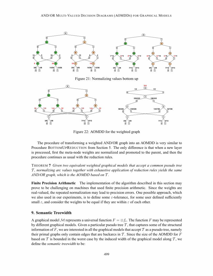
AND/OR MULTI-VALUED DECISION DIAGRAMS (AOMDDS) FOR GRAPHICAL MODELS
0
A
B
0
C
0 1
1
1
0
M
1
C
0 1
B
0 1
0
A
B
0
C
0 1
1
1
C
0 1
B
0 1
3/8 5/8 14/26 12/26 3/8 5/8 14/26 12/26
12 5 18 2 4 10 6 4
8 26 24 13
0
A
B
0
C
0 1
1
1
0
M
1
C
0 1
B
0 1
0
A
B
0
C
0 1
1
1
C
0 1
B
0 1
3/8 5/8 7/13 6/13 3/8 5/8 7/13 6/13
8*12 26*5 8*18 26*2 24*4 13*10 24*6 13*4
Figure 21: Normalizing values bottom up
0
A
B
0
C
0 1
1
1
0
M
1
C
0 1
B
0 1
0
A
B
0 1
1
B
0 1
3/8 5/8 7/13 6/13
96 130 144 52 96 130 144 52
0
A
B
0
C
0 1
1
1
0
M
1
C
0 1
B
0 1
3/8 5/8 7/13 6/13
226/422 196/422
1/2 1/2
96/226 130/226 144/196 52/196
844
Figure 22: AOMDD for the weighted graph
The procedure of transforming a weighted AND/OR graph into an AOMDD is very similar toProcedure BOTTOMUPREDUCTION from Section 5. The only difference is that when a new layeris processed, first the meta-node weights are normalized and promoted to the parent, and then theprocedure continues as usual with the reduction rules.
THEOREM 7 Given two equivalent weighted graphical models that accept a common pseudo treeT , normalizing arc values together with exhaustive application of reduction rules yields the sameAND/OR graph, which is the AOMDD based on T .
Finite Precision Arithmetic The implementation of the algorithm described in this section mayprove to be challenging on machines that used finite precision arithmetic. Since the weights arereal-valued, the repeated normalization may lead to precision errors. One possible approach, whichwe also used in our experiments, is to define some ε-tolerance, for some user defined sufficientlysmall ε, and consider the weights to be equal if they are within ε of each other.
9. Semantic Treewidth
A graphical modelM represents a universal function F = ⊗fi. The function F may be representedby different graphical models. Given a particular pseudo tree T , that captures some of the structuralinformation ofF , we are interested in all the graphical models that accept T as a pseudo tree, namelytheir primal graphs only contain edges that are backarcs in T . Since the size of the AOMDD for Fbased on T is bounded in the worst case by the induced width of the graphical model along T , wedefine the semantic treewidth to be:
499

MATEESCU, DECHTER & MARINESCU
�
��
�
��
����
�
��
�
��
����
(a) The two solutions
A
DB
C
�������������
������������������
�������������������� �
�������������
����������������
������������ �
(b) First model
A DB C
�����
�����
���� �
(c) Second model
Figure 23: The 4-queen problem
DEFINITION 27 (semantic treewidth) The semantic treewidth of a graphical model M relativeto a pseudo tree T denoted by swT (M), is the smallest treewidth taken over all models R thatare equivalent to M, and accept the pseudo tree T . Formally, it is defined by swT (M) =minR,u(R)=u(M)wT (R), where u(M) is the universal function ofM, and wT (R) is the inducedwidth of R along T . The semantic treewidth of a graphical model, M, is the minimal semantictreewidth over all the pseudo trees that can express its universal function.
Computing the semantic treewidth can be shown to be NP-hard.3
THEOREM 8 Computing the semantic treewidth of a graphical modelM is NP-hard.
Theorem 8 shows that computing the semantic treewidth is hard, and it is likely that the actualcomplexity is even higher. However, the semantic treewidth can explain why sometimes the minimalAND/OR graph or OBDD are much smaller than the exponential in treewidth or pathwidth upperbounds. In many cases, there could be a huge disparity between the treewidth ofM and the semantictreewidth along T .
Example 14 Figure 23(a) shows the two solutions of the 4-queen problem. The problem is ex-pressed by a complete graph of treewidth 3, given in Figure 23(b). Figure 23(c) shows an equivalentproblem (i.e., that has the same set of solutions), which has treewidth 1. The semantic treewidth ofthe 4-queen problem is 1.
Based on the fact that an AOMDD is a canonical representation of the universal function of agraphical model, we can conclude that the size of the AOMDD is bounded exponentially by thesemantic treewidth along the pseudo tree, rather than the treewidth of the given graphical modelrepresentation.
Proposition 7 The size of the AOMDD of a graphical model M is bounded by O(n kswT (M)),where n is the number of variables, k is the maximum domain size and swT (M) is the semantictreewidth ofM along the pseudo tree T .
3. We thank David Eppstein for the proof.
500

AND/OR MULTI-VALUED DECISION DIAGRAMS (AOMDDS) FOR GRAPHICAL MODELS
0 1
A
B B
C C
D D
(a) OBDD representation
A
B M
C N
D P
(b) Primal graph with hiddenvariablesM, N and P .
Figure 24: The parity function
Example 15 Consider a constraint network on n variables such that every two variables are con-strained by equality (X = Y ). One graph representation is a complete graph, another is a chainand another is a tree. If the problem is specified as a complete graph, and if we use a linear order,the OBDD will have a linear size because there exists a representation having a pathwidth of 1(rather than n).
While the semantic treewidth can yield a much better upper bound on the AOMDD, it can alsobe a very bad bound. It is well known that the parity function on n variables has a very compact,chain-like OBDD representation. Yet, the only constraint network representation of a parity functionis the function itself (namely a complete graph on all the variables), whose treewidth and semantictreewidth is its number of variables, n. The OBDD representation of the parity function suggeststhat the addition of hidden variables can simplify its presentation. We show an example in Figure24. On the left side, in Figure 24(a) we have the OBDD representation of the parity function forfour binary variables. A graphical model would represent this function by a complete graph on thefour variables. However, we could add the extra variablesM, N and P in Figure 24(b), sometimescalled “hidden” variables, that can help decompose the model. In this caseM can form a constrainttogether with A and B such thatM represents the parity of A and B, namelyM = 1 if A⊕B = 1,where ⊕ is the parity (XOR) operator. Similarly, N would capture the parity of M and C, and P
would capture the parity of N and D, and would also give the parity of the initial four variables.The two structures are surprisingly similar. It would be interesting to study further the connectionbetween hidden variables and compact AOBDDs, but we leave this for future work.
10. Experimental Evaluation
Our experimental evaluation is in preliminary stages, but the results we have are already encourag-ing. We ran the search-based compile algorithm, by recording the trace of the AND/OR search, andthen reducing the resulting AND/OR graph bottom up. In these results we only applied the reduc-tion by isomorphism and still kept the redundant meta-nodes. We implemented our algorithms inC++ and ran all experiments on a 2.2GHz Intel Core 2 Duo with 2GB of RAM, running Windows.
501

MATEESCU, DECHTER & MARINESCU
10.1 Benchmarks
We tested the performance of the search-based compilation algorithm on random Bayesian net-works, instances from the Bayesian Network Repository and a subset of networks from the UAI’06Inference Evaluation Dataset.
Random Bayesian Networks The random Bayesian networks were generated using parameters(n, k, c, p), where n is the number of variables, k is the domain size, c is the number of conditionalprobability tables (CPTs) and p is the number of parents in each CPT. The structure of the networkwas created by randomly picking c variables out of n and, for each, randomly picking p parents fromtheir preceding variables, relative to some ordering. The remaining n − c variables are called rootnodes. The entries of each probability table were generated randomly using a uniform distribution,and the table was then normalized. It is also possible to control the amount of determinism in thenetwork by forcing a percentage det of the CPTs to have only 0 and 1 entries.
Bayesian Network Repository The Bayesian Network Repository4 contains a collection of beliefnetworks extracted from various real-life domains which are often used for benchmarking proba-bilistic inference algorithms.
UAI’06 Inference Evaluation Dataset The UAI 2006 Inference Evaluation Dataset5 contains acollection of random as well as real-world belief networks that were used during the first UAI 2006Inference Evaluation contest. For our purpose we selected a subset of networks which were derivedfrom the ISCAS’89 digital circuits benchmark.6 ISCAS’89 circuits are a common benchmark usedin formal verification and diagnosis. Each of these circuits was converted into a Bayesian networkby removing flip-flops and buffers in a standard way, creating a deterministic conditional probabilitytable for each gate, and putting uniform distributions on the input signals.
10.2 Algorithms
We consider two search-based compilation algorithms, denoted by AOMDD-BCP and AOMDD-SAT, respectively, that reduce the context minimal AND/OR graph explored via isomorphism, whileexploiting the determinism (if any) present in the network. The approach we take for handling thedeterminism is based on unit resolution over a CNF encoding (i.e., propositional clauses) of the zeroprobability tuples of the CPTs. The idea of using unit resolution during search for Bayesian net-works was first explored by Allen and Darwiche (2003). AOMDD-BCP is conservative and appliesonly unit resolution at each node in the search graph, whereas AOMDD-SAT is more aggressive anddetects inconsistency by running a full SAT solver. We used the zChaff SAT solver (Moskewicz,Madigan, Zhao, Zhang, & Malik, 2001) for both unit resolution as well as full satisfiability. Forcomparison, we also ran an OR version of AOMDD-BCP, called MDD-BCP.For reference we also report results obtained with the ACE7 compiler. ACE compiles a Bayesian
network into an Arithmetic Circuit (AC) and then uses the AC to answer multiple queries with re-spect to the network. An arithmetic circuit is a representation that is equivalent to AND/OR graphs(Mateescu & Dechter, 2007). Each time ACE compiler is invoked, it uses one of two algorithmsas the basis for compilation. First, if an elimination order can be generated for the network having
4. http://www.cs.huji.ac.il/compbio/Repository/5. http://ssli.ee.washington.edu/bilmes/uai06InferenceEvaluation6. Available at: http://www.fm.vslib.cz/kes/asic/iscas/7. Available at: http://reasoning.cs.ucla.edu/ace
502

AND/OR MULTI-VALUED DECISION DIAGRAMS (AOMDDS) FOR GRAPHICAL MODELS
Network (w*, h) (n, k) ACE MDD w/ BCP AOMDD w/ BCP AOMDD w/ SAT#nodes time #meta #cm(OR) time #meta #cm(OR) time #meta #cm(OR) time
Bayesian Network Repositoryalarm (4, 13) (37, 4) 1,511 0.01 208,837 682,195 73.35 320 459 0.05 320 459 0.22cpcs54 (14, 23) (54, 2) 196,933 0.06 - - - 65,158 66,405 6.97 65,158 66,405 6.97cpcs179 (8, 14) (179, 4) 67,919 0.05 - - - 9,990 32,185 46.56 9,990 32,185 46.56cpcs360b (20, 27) (360, 2) 5,258,826 1.72 - - - - - - - - -diabetes (4, 77) (413, 21) 7,615,989 1.81 - - - - - - - - -hailfinder (4, 16) (56, 11) 8,815 0.01 - - - 2,068 2,202 0.34 1,893 2,202 1.48mildew (4, 13) (35, 100) 823,913 0.39 - - - 73,666 110,284 1367.81 62,903 65,599 3776.82mm (20, 57) (1220, 2) 47,171 1.49 - - - 38,414 58,144 4.54 30,274 52,523 99.55munin2 (9, 32) (1003, 21) 2,128,147 1.91 - - - - - - - - -munin3 (9, 32) (1041, 21) 1,226,635 1.27 - - - - - - - - -munin4 (9, 32) (1044, 21) 2,423,009 4.44 - - - - - - - - -pathfinder (6, 11) (109, 63) 18,250 0.05 610,854 1,303,682 352.18 6,984 16,267 30.71 2,265 15,963 50.36pigs (11, 26) (441, 3) 636,684 0.19 - - - 261,920 294,101 174.29 198,284 294,101 1277.72water (10, 15) (32, 4) 59,642 0.52 707,283 1,138,096 95.14 18,744 20,926 2.02 18,503 19,225 7.45
UAI’06 Evaluation DatasetBN 42 (21, 62) (851, 2) 4,860 1.35 - - - 107,025 341,428 53.50 42,445 43,280 57.36BN 43 (26, 65) (851, 2) 10,373 1.62 - - - 1,343,923 1,679,013 1807.63 313,388 314,669 434.38BN 44 (25, 56) (851, 2) 4,235 1.31 - - - 155,588 187,589 20.90 47,222 48,540 66.09BN 45 (22, 54) (851, 2) 12,319 1.50 - - - 390,795 487,593 68.81 126,182 126,929 177.50BN 46 (20, 46) (851, 2) 5,912 2.90 1,125,658 1,228,332 94.93 16,711 17,532 1.31 7,337 7,513 5.54BN 47 (39, 57) (632, 2) 1,448 1.17 42,419 47,128 2.87 1,873 2,663 0.24 1,303 2,614 2.36BN 49 (40, 60) (632, 2) 1,408 1.16 18,344 19,251 1.32 1,205 1,539 0.19 952 1,515 1.34BN 51 (41, 68) (632, 2) 1,467 1.15 63,851 68,005 4.22 4,442 5,267 0.50 3,653 5,195 4.58BN 53 (47, 87) (532, 2) 1,357 0.91 14,210 19,162 1.49 4,819 9,561 0.74 1,365 1,719 1.36BN 55 (49, 92) (532, 2) 1,288 0.93 5,168 6,088 0.57 1,972 2,816 0.26 790 904 0.75BN 57 (49, 85) (532, 2) 1,276 0.90 48,436 51,611 3.52 4,036 5,089 0.37 962 1,277 1.01BN 59 (52, 87) (511, 2) 1,749 0.93 332,030 353,720 25.61 22,963 29,146 2.14 10,655 18,752 14.17BN 61 (41, 64) (638, 2) 1,411 1.10 20,459 20,806 1.45 1,244 1,589 0.17 1,016 1,528 1.37BN 63 (53, 95) (511, 2) 1,324 0.90 11,461 17,087 1.28 7,182 14,048 1.07 1,419 2,177 1.69BN 65 (56, 86) (411, 2) 1,184 0.75 - - - 20,764 23,102 1.52 12,569 19,778 12.90BN 67 (54, 88) (411, 2) 1,031 0.74 - - - 179,067 511,031 154.91 716 1,169 0.78
Positive Random Bayesian Networks (n=75, k=2, p=2, c=65)r75-1 (12, 22) (75, 2) 67,737 0.31 - - - 21,619 21,619 2.59 21,619 21,619 2.59r75-2 (12, 23) (75, 2) 46,703 0.29 - - - 18,083 18,083 1.88 18,083 18,083 1.88r75-3 (11, 26) (75, 2) 53,245 0.30 - - - 18,419 18,419 1.86 18,419 18,419 1.86r75-4 (11, 19) (75, 2) 28,507 0.29 - - - 8,363 8,363 1.16 8,363 8,363 1.16r75-5 (13, 24) (75, 2) 149,707 0.36 - - - 42,459 42,459 4.61 42,459 42,459 4.61r75-6 (14, 24) (75, 2) 132,107 1.19 - - - 62,621 62,621 6.95 62,621 62,621 6.95r75-7 (12, 24) (75, 2) 89,913 0.36 - - - 21,583 21,583 2.42 21,583 21,583 2.42r75-8 (14, 24) (75, 2) 86,183 0.36 - - - 49,001 49,001 6.23 49,001 49,001 6.23r75-9 (11, 19) (75, 2) 29,025 0.30 - - - 7,681 7,681 0.81 7,681 7,681 0.81r75-10 (10, 24) (75, 2) 20,291 0.28 - - - 5,905 5,905 0.63 5,905 5,905 0.63Deterministic Random Bayesian Networks (n=100, k=2, p=2, c=90) and det = 25% of the CPTs containing only 0 and 1 entries
r100d25-1 (13, 31) (100, 2) 68,398 0.38 - - - 34,035 34,075 2.94 34,035 34,075 12.77r100d25-2 (16, 28) (100, 2) 150,134 0.46 - - - 70,241 70,931 7.72 70,241 70,931 27.17r100d25-3 (16, 29) (100, 2) 705,200 0.96 - - - 134,079 135,203 13.80 134,079 135,203 50.51r100d25-4 (16, 31) (100, 2) 161,902 0.54 - - - 79,366 79,488 7.26 79,366 79,488 28.06r100d25-5 (16, 29) (100, 2) 185,348 0.53 - - - 140,627 140,636 14.57 140,627 140,636 49.42r100d25-6 (18, 28) (100, 2) 148,835 0.66 - - - 204,232 210,066 17.56 197,134 210,066 92.24r100d25-7 (16, 29) (100, 2) 264,629 0.60 - - - 134,344 135,008 14.26 133,850 135,008 55.60r100d25-8 (17, 27) (100, 2) 65,186 0.46 - - - 36,857 36,887 2.95 36,857 36,887 11.97r100d25-9 (14, 27) (100, 2) 140,014 0.40 - - - 58,421 59,791 6.88 58,172 59,791 23.21r100d25-10 (16, 27) (100, 2) 173,808 0.58 - - - 69,110 69,136 7.50 69,110 69,136 26.50
Table 1: Results for experiments with 50 Bayesian networks from 3 problem classes; w∗ =treewidth, h = depth of pseudo tree, n = number of variables, k = domain size, time
given in seconds; bold types highlight the best results across rows.
503

MATEESCU, DECHTER & MARINESCU
sufficiently small induced width, then tabular variable elimination will be used as the basis. Thisalgorithm is similar to the one discussed by Chavira and Darwiche (2007), but uses tables to rep-resent factors rather than ADDs. If the induced width is large, then logical model counting will beused as the basis. Tabular variable elimination is typically efficient when width is small but cannothandle networks when the width is larger. Logical model counting, on the other hand, incurs moreoverhead than tabular variable elimination, but can handle many networks having larger treewidth.Both tabular variable elimination and logical model counting produce ACs that exploit local struc-ture, leading to efficient online inference. When logical model counting is invoked, it proceedsby encoding the Bayesian network into a CNF (Chavira & Darwiche, 2005; Chavira, Darwiche, &Jaeger, 2006), simplifying the CNF, compiling the CNF into a d-DNNF, and then extracting the ACfrom the compiled d-DNNF. A dtree over the CNF clauses drives the compilation step.In all our experiments we report the compilation time in seconds (time), the number of OR
nodes in the context minimal graph explored (#cm), the number of meta-nodes of the resultingAOMDD (#meta), as well as the size of the AC compiled by ACE (#nodes). For each network wespecify the number of variables (n), domain size (k), induced width (w∗) and pseudo tree depth (h).A ’-’ stands for exceeding the 2GBmemory limit by the respective algorithm. The best performancepoints are highlighted.
10.3 Evaluation on Bayesian Networks
Table 1 reports the results obtained for experiments with 50 Bayesian networks. The AOMDDcompilers as well as ACE used the min-fill heuristic (Kjæaerulff, 1990) to construct the guidingpseudo tree and dtree, respectively.
10.3.1 BAYESIAN NETWORKS REPOSITORY
We see that ACE is overall the fastest compiler on this domain, outperforming both AOMDD-BCPand AOMDD-SAT with up to several orders of magnitude (e.g., mildew, pigs). However, thediagrams compiled by ACE and AOMDD-BCP (resp. AOMDD-SAT) are comparable in size. Insome cases, AOMDD-BCP and AOMDD-SAT were able to compile much smaller diagrams thanACE. For example, the diagram produced by AOMDD-BCP for the mildew network is 13 timessmaller than the one compiled by ACE. In principle the output produced by ACE and AOMDDshould be similar if both are guided by the same pseudo tree/dtree. Our scheme should be viewedas a compilation alternative which (1) extends decision diagrams and (2) mimics traces of searchproperties that may make this representation accessible. The OR compiler MDD-BCP was ableto compile only 3 out of the 14 test instances, but their sizes were far larger than those producedby AOMDD-BCP. For instance, on the pathfinder network, AOMDD-BCP outputs a decisiondiagram almost 2 orders of magnitude smaller than MDD-BCP.
10.3.2 UAI’06 DATASET
For each of the UAI’06 Dataset instances we picked randomly 30 variables and instantiated asevidence. We see that ACE is the best performing compiler on this dataset. AOMDD-BCP iscompetitive with ACE in terms of compile time only on 9 out the 16 test instances. AOMDD-SATis able to compile the smallest diagrams for 6 networks only (e.g., BN 47, BN 49, BN 55, BN 57,BN 61, BN 67). As before, the difference in size between the compiled data-structures producesby MDD-BCP and AOMDD-BCP is up to 2 orders of magnitude in favor of the latter.
504

AND/OR MULTI-VALUED DECISION DIAGRAMS (AOMDDS) FOR GRAPHICAL MODELS
10.3.3 RANDOM NETWORKS
The problem instances denoted by r75-1 through r75-10 were generated from a class of randombelief networks with parameters (n = 75, k = 2, p = 2, c = 65). Similarly, the instances denotedby r100d25-1 through r100d25-10 belong to a class with parameters (n = 100, k = 2, p = 2, c =90). In the latter case, det = 25% of the CPTs are deterministic, namely they contain only 0 and1 probability tuples. These test instances were compiled without any evidence. We see that on thisdomain AOMDD-BCP/AOMDD-SAT were able to compile the smallest diagrams, which were onaverage about 2 times smaller than those produced by ACE. However, ACE was again the fastestcompiler. Notice that the OR compiler MDD-BCP ran out of memory in all test cases.
10.4 The Impact of Variable Ordering
As theory dictates, the AOMDD size is influenced by the quality of the guiding pseudo tree. Inaddition to the min-fill heuristic we also considered the hypergraph heuristic which constructs thepseudo tree by recursively decomposing the dual hypergraph associated with the graphical model.This idea was also explored by Darwiche (2001) for constructing dtrees that guide ACE.Since both the min-fill and hypergraph partitioning heuristics are randomized (namely ties are
broken randomly), the size of the AOMDD guided by the resulting pseudo tree may vary signifi-cantly from one run to the next. Figure 25 displays the AOMDD size using hypergraph and min-fillbased pseudo trees for 6 networks selected from Table 1, over 20 independent runs. We also recordthe average induced width and depth obtained for the pseudo trees (see the header of each plot inFigure 25). We see that the two heuristics do not dominate each other, namely the variance in outputsize is quite significant in both cases.
10.5 Memory Usage
Table 2 shows the memory usage (in MBytes) of ACE, AOMDD-BCP and AOMDD-SAT, respec-tively, on the Bayesian networks from Table 1. We see that in some cases the AOMDD based com-pilers require far less memory than ACE. For example, on the “mildew” network, both AOMDD-BCP and AOMDD-SAT use about 22 MB of memory to compile the AND/OR decision diagram,while ACE requires as much as 218 MB of memory. Moreover, the compiled AOMDD has in thiscase about one order of magnitude fewer nodes than that constructed by ACE. When comparing thetwo AND/OR search-based compilers, we observe that on networks with a significant amount ofdeterminism, such as those from the UAI’06 Evaluation dataset, AOMDD-SAT uses on average twotimes less memory than AOMDD-BCP. The most dramatic savings in memory usage due to the ag-gressive constraint propagation employed by AOMDD-SAT compared with AOMDD-BCP can beseen on the “BN 67” network. In this case, the difference in memory usage between AOMDD-SATand AOMDD-BCP is about 2 orders of magnitude in favor of the former.
11. Related Work
The related work can be viewed along two directions: (1) the work related to the AND/OR searchidea for graphical models and (2) the work related to compilation for graphical models that exploitsproblem structure.An extensive discussion for (1) was provided in the previous work of Dechter and Mateescu
(2007). Since this is not the focus of the paper, we just mention that the AND/OR idea was origi-
505

MATEESCU, DECHTER & MARINESCU
Figure 25: Effect of variable ordering.
506

AND/OR MULTI-VALUED DECISION DIAGRAMS (AOMDDS) FOR GRAPHICAL MODELS
Network ACE AOMDD w/ BCP AOMDD w/ SAT#nodes memory (MB) #nodes memory (MB) #nodes memory (MB)
Bayesian Network Repositoryalarm 1,511 0.00 320 0.0206 320 0.0206cpcs54 196,933 4.00 65,158 3.4415 65,158 3.4415cpcs179 67,919 5.00 9,990 1.9263 9,990 1.9263cpcs360b 5,258,826 204.00 - - - -diabetes 7,615,989 449.00 - - - -hailfinder 8,815 0.00 2,068 0.1576 1,893 0.1740mildew 823,913 218.00 73,666 22.5781 62,903 22.1467mm 47,171 369.00 38,414 1.5719 30,274 1.3711munin2 2,128,147 202.00 - - - -munin3 1,226,635 150.00 - - - -munin4 2,423,009 n/a - - - -pathfinder 18,250 10.00 6,984 0.6009 2,265 0.3515pigs 636,684 31.00 261,920 23.3761 198,284 17.7096water 59,642 161.00 18,744 1.09578 18,503 1.3258
UAI’06 Evaluation DatasetBN 42 4,860 n/a 107,025 4.5622 42,445 1.9323BN 43 10,373 n/a 1,343,923 57.8422 313,388 14.2828BN 44 4,235 n/a 155,588 6.5613 47,222 2.1628BN 45 12,319 n/a 390,795 17.9325 126,182 5.7958BN 46 5,912 n/a 16,711 0.6929 7,337 0.3401BN 47 1,448 n/a 1,873 0.0720 1,303 0.0583BN 49 1,408 n/a 1,205 0.0449 952 0.0409BN 51 1,467 n/a 4,442 0.1689 3,653 0.1633BN 53 1,357 n/a 4,819 0.1814 1,365 0.0587BN 55 1,288 n/a 1,972 0.0723 790 0.0336BN 57 1,276 n/a 4,036 0.1495 962 0.0411BN 59 1,749 n/a 22,963 0.8501 10,655 0.4587BN 61 1,411 n/a 1,244 0.0463 1,016 0.0445BN 63 1,324 n/a 7,182 0.2728 1,419 0.0607BN 65 1,184 n/a 20,764 0.7539 12,569 0.5384BN 67 1,031 n/a 179,067 6.9603 716 0.0304
Positive Random Bayesian Networks with parameters (n=75, k=2, p=2, c=65)r75-1 67,737 1.00 21,619 1.2503 21,619 1.2503r75-2 46,703 1.00 18,083 0.9957 18,083 0.9957r75-3 53,245 1.00 18,419 0.9955 18,419 0.9955r75-4 28,507 1.00 8,363 0.5171 8,363 0.5171r75-5 149,707 3.00 42,459 2.3299 42,459 2.3299r75-6 132,107 3.00 62,621 3.4330 62,621 3.4330r75-7 89,913 2.00 21,583 1.1942 21,583 1.1942r75-8 86,183 2.00 49,001 2.8130 49,001 2.8130r75-9 29,025 1.00 7,681 0.4124 7,681 0.4124r75-10 20,291 1.00 5,905 0.3261 5,905 0.3261Deterministic Random Bayesian Networks with parameters (n=100, k=2, p=2, c=90)r100d25-1 68,398 5.00 34,035 1.6290 34,035 1.7149r100d25-2 150,134 10.00 70,241 3.6129 70,241 3.7810r100d25-3 705,200 40.00 134,079 6.6372 134,079 6.9873r100d25-4 161,902 22.00 79,366 3.8113 79,366 4.0079r100d25-5 185,348 15.00 140,627 7.0839 140,627 7.4660r100d25-6 148,835 37.00 204,232 9.1757 197,134 9.6542r100d25-7 264,629 19.00 134,344 6.9619 133,850 6.9961r100d25-8 65,186 21.00 36,857 1.6872 36,857 1.8278r100d25-9 140,014 6.00 58,421 3.1058 58,172 3.2055r100d25-10 173,808 27.00 69,110 3.5578 69,110 3.6636
Table 2: Memory usage in MBytes of ACE, AOMDD-BCP and AOMDD-SAT on the 50 Bayesiannetworks from Table 1. Bold types highlight the best performance across rows. The “n/a”indicates that the respective memory usage statistic was not available from ACE’s output.
507

MATEESCU, DECHTER & MARINESCU
nally developed for heuristic search (Nilsson, 1980). As mentioned in the introduction, the AND/ORsearch for graphical models is based on a pseudo tree that spans the graph of the model, similar tothe tree rearrangement of Freuder and Quinn (1985, 1987). The idea was adapted for distributedconstraint satisfaction by Collin et al. (1991, 1999) and more recently by Modi et al. (2005), and wasalso shown to be related to graph-based backjumping (Dechter, 1992). This work was extended byBayardo and Miranker (1996), Bayardo and Schrag (1997) and more recently applied to optimiza-tion tasks by Larrosa et al. (2002). Another version that can be viewed as exploring the AND/ORgraphs was presented recently for constraint satisfaction (Terrioux & Jegou, 2003b) and for opti-mization (Terrioux & Jegou, 2003a). Similar principles were introduced recently for probabilisticinference, in algorithm Recursive Conditioning (Darwiche, 2001) as well as in Value Elimination(Bacchus et al., 2003b, 2003a), and are currently at the core of the most advanced SAT solvers (Sanget al., 2004).For direction (2), there are various lines of related research. The formal verification literature,
beginning with the work of Bryant (1986) contains a very large number of papers dedicated to thestudy of BDDs. However, BDDs are in fact OR structures (the underlying pseudo tree is a chain)and do not take advantage of the problem decomposition in an explicit way. The complexity boundsfor OBDDs are based on pathwidth rather than treewidth.As noted earlier, the work of Bertacco and Damiani (1997) on Disjoint Support Decomposition
(DSD) is related to AND/OR BDDs in various ways. The main common aspect is that both ap-proaches show how structure decomposition can be exploited in a BDD-like representation. DSDis focused on Boolean functions and can exploit more refined structural information that is inher-ent to Boolean functions. In contrast, AND/OR BDDs assume only the structure conveyed in theconstraint graph, and are therefore more broadly applicable to any constraint expression and alsoto graphical models in general. They allow a simpler and higher level exposition that yields graph-based bounds on the overall size of the generated AOMDD. The full relationship between these twoformalisms should be studied further.McMillan (1994) introduced the BDD trees, along with the operations for combining them. For
circuits of bounded tree width, BDD trees have a linear space upper bound of O(|g|2w22w), where
|g| is the size of the circuit g (typically linear in the number of variables) andw is the treewidth. Thisbound hides some very large constants to claim the linear dependence on |g| when w is bounded.However, McMillan maintains that when the input function is a CNF expression BDD-trees havethe same bounds as AND/OR BDDs, namely they are exponential in the treewidth only.To sketch just a short comparison between McMillan’s BDD trees and AOMMDs, consider an
example where we have a simple pseudo tree with root α, left child β and right child γ. Each ofthese nodes may stand for a set of variables. In BDD trees, the assignments to β are grouped intoequivalence classes according to the cofactors generated by them on the remaining α and γ. Forexample assignments β1 and β2 are equivalent if they generate the same function on α and γ. Thenode β can be represented by a BDD whose leaves are the cofactors. The same is done for γ. Thenode α is then represented by a matrix of BDDs, where each column corresponds to a cofactor of βand each line to a cofactor of γ. By contrast, an AOMDD represents the node α as a BDD whoseleaves are the cofactors (the number of distinct functions on β and γ) and then each cofactor is theroot of a decomposition (an AND node) between β and γ. Moreover, the representations of β (asdescendants of different cofactor of α) are shared as much as possible and the same goes for γ. Thisis only a high level description, that becomes slightly more complicated when redundant nodes areeliminated, but the idea remains the same.
508

AND/OR MULTI-VALUED DECISION DIAGRAMS (AOMDDS) FOR GRAPHICAL MODELS
The AND/OR structure restricted to propositional theories is very similar to deterministic de-composable negation normal form (d-DNNF) (Darwiche & Marquis, 2002; Darwiche, 2002). Morerecently, Huang and Darwiche (2005b) used the trace of the DPLL algorithm to generate an OBDD,and compared with the typical formal verification approach of combining the OBDDs of the inputfunction according to some schedule. The structures that were investigated in that case are still OR.This idea is extended in our present work by the AND/OR search compilation algorithm.McAllester, Collins, and Pereira (2004) introduced the case factor diagrams (CFD), which sub-
sumeMarkov random fields of bounded tree width and probabilistic context free grammars (PCFG).CFDs are very much related to the AND/OR graphs. The CFDs target the minimal representation,by exploiting decomposition (similar to AND nodes) but also by exploiting context sensitive infor-mation and allowing dynamic ordering of variables based on context. CFDs do not eliminate theredundant nodes, and part of the cause is that they use zero suppression. There is no claim aboutCFDs being canonical forms, and also no description of how to combine two CFDs.There are numerous variants of decision diagrams that are designed to represent integer-valued
or real-valued functions. For a comprehensive view we refer the reader to the survey of Drechslerand Sieling (2001). Algebraic decision diagrams (ADDs) (Bahar et al., 1993) provide a compi-lation for general real-valued rather than Boolean functions. Their main drawback is that theirsize increases very fast if the number of terminals becomes large. There are several approachesthat try to alleviate this problem. However the structure that they capture is still OR, and theydo not exploit decomposition. Some alternatives introduce edge values (or weights) that enablemore subgraph sharing. Edge-valued binary decision diagrams (EVBDDs) (Lai & Sastry, 1992)use additive weights, and when multiplicative weights are also allowed they are called factoredEVBDDs (FEVBDDs) (Tafertshofer & Pedram, 1997). Another type of BDDs called K*BMDs(Drechsler, Becker, & Ruppertz, 1996) also use integer weights, both additive and multiplicativein parallel. ADDs have also been extended to affine ADDs (Sanner & McAllester, 2005), throughaffine transformations that can achieve more compression. The result was shown to be beneficialfor probabilistic inference algorithms, such as tree clustering, but they still do not exploit the ANDstructure.More recently, independently and in parallel to our work on AND/OR graphs (Dechter & Ma-
teescu, 2004a, 2004b), Fargier and Vilarem (2004) and Fargier and Marquis (2006, 2007) pro-posed the compilation of CSPs into tree-driven automata, which have many similarities to our work.Their main focus is the transition from linear automata to tree automata (similar to that from ORto AND/OR), and the possible savings for tree-structured networks and hyper-trees of constraintsdue to decomposition. Their compilation approach is guided by a tree-decomposition while ours isguided by a variable-elimination based algorithms. And it is well known that Bucket Eliminationand cluster-tree decomposition are in principle the same (Dechter & Pearl, 1989).Wilson (2005) extended OBDDs to semi-ring BDDs. The semi-ring treatment is restricted to
the OR search spaces, but allows dynamic variable ordering. It is otherwise very similar in aim andscope to our AOMDD.When restricting the AOMDD to OR graphs only, the two are closely related,except that we express BDDs using the Shenoy-Shafer axiomatization that is centered on the twooperation of combination and marginalization rather then on the semi-ring formulation. Minimalityin the formulation of Wilson (2005) is more general allowing merging nodes having different valuesand therefore it can capture symmetries (called interchangeability).Another framework very similar to AOMDDs, that we became aware of only recently, is Prob-
abilistic Decision Graphs (PDG) of Jaeger (2004). This work preceded most of the relevant work
509

MATEESCU, DECHTER & MARINESCU
we discussed above (Fargier & Vilarem, 2004; Wilson, 2005) and went somewhat unnoticed, per-haps due to notational and cultural differences. It is however similar in motivation, framework andproposed algorithms. We believe our AND/OR framework is more accessible. We define the frame-work over multi-valued domains, provide greater details in algorithms and complexity analysis,make an explicit connection with search frameworks, fully address the issues of canonicity as wellas provide an empirical demonstration. In particular, the claim of canonicity for PDGs is similar tothe one we make for AOMDDs of weighted models, in that it is relative to the trees (or forests) thatcan represent the given probability distribution.There is another line of research by Drechsler and his group (e.g. Zuzek, Drechsler, & Thornton,
2000), who use AND/OR graphs for Boolean function representation, that may seem similar to ourapproach. However, the semantics and purpose of their AND/OR graphs are different. They areconstructed based on the technique of recursive learning and are used to perform Boolean reasoning,i.e. to explore the logic consequences of a given assumption based on the structure of the circuit,especially to derive sets of implicants. The meaning of AND and OR in their case is related tothe meaning of the gates/functions, while in our case the meaning is not related to the semantic ofthe functions. The AND/OR enumeration tree that results from a circuit according to Zuzek et al.(2000) is not related to the AND/OR decomposition that we discuss.
12. Conclusion
We propose the AND/OR multi-valued decision diagram (AOMDD), which emerges from the studyof AND/OR search spaces for graphical models (Dechter & Mateescu, 2004a, 2004b; Mateescu &Dechter, 2005; Dechter &Mateescu, 2007) and ordered binary decision diagrams (OBDDs) (Bryant,1986). This data-structure can be used to compile any graphical model.Graphical models algorithms that are search-based and compiled data-structures such as BDDs
differ primarily by their choices of time vs. memory. When we move from regular OR searchspace to an AND/OR search space the spectrum of algorithms available is improved for all timevs. memory decisions. We believe that the AND/OR search space clarifies the available choicesand helps guide the user into making an informed selection of the algorithm that would fit best theparticular query asked, the specific input function and the available computational resources.The contribution of our work is: (1) We formally describe the AOMDD and prove that it is a
canonical representation of a constraint network. (2) We extend the AOMDD to general weightedgraphical models. (3) We give a compilation algorithm based on AND/OR search, that saves thetrace of a memory intensive search (the context minimal AND/OR graph), and then reduces itin one bottom up pass. (4) We describe the APPLY operator that combines two AOMDDs by anoperation and show that its complexity is quadratic in the input, but never worse than exponentialin the treewidth. (5) We give a scheduling order for building the AOMDD of a graphical modelstarting with the AOMDDs of its functions which is based on a Variable Elimination algorithm.This guarantees that the complexity is at most exponential in the induced width (treewidth) along theordering. (6) We show how AOMDDs relate to various earlier and recent compilation frameworks,providing a unifying perspective for all these methods. (7) We introduce the semantic treewidth,which helps explain why compiled decision diagrams are often much smaller than the worst casebound. Finally, (8) we provide a preliminary empirical demonstration of the power of the currentscheme.
510

AND/OR MULTI-VALUED DECISION DIAGRAMS (AOMDDS) FOR GRAPHICAL MODELS
Acknowledgments
This work was done while Robert Mateescu and Radu Marinescu were at the University of Cal-ifornia, Irvine. The authors would like to thank the anonymous reviewers for their constructivesuggestions to improve the paper, David Eppstein for a useful discussion of complexity issues, andLars Otten and Natasha Flerova for comments on the final version of the manuscript. This work wassupported by the NSF grants IIS-0412854 and IIS-0713118, and the initial part by the Radcliffe fel-lowship 2005-2006 (through the partner program), with Harvard undergraduate student John Cobb.
Appendix
Proof of Proposition 1Consider the level of variable Xi, and the meta-nodes in the list LXi . After one pass through themeta-nodes in LXi (the inner for loop), there can be no two meta-nodes at the level of Xi in theAND/OR graph that are isomorphic, because they would have been merged in line 6. Also, duringthe same pass through the meta-nodes in LXi all the redundant meta-nodes in LXi are eliminatedin line 8. Processing the meta-nodes in the level of Xi will not create new redundant or isomorphicmeta-nodes in the levels that have been processed before. It follows that the resulting AND/ORgraph is completely reduced. �
Proof of Theorem 4The bound on the size follows directly from Theorem 3. The AOMDD size can only be smaller thanthe size of the context minimal AND/OR graph, which is bounded by O(n kw∗
T(G)). To prove the
time bound, we have to rely on the use of the hash table, and the assumption that an efficient imple-mentation allows an access time that is constant. The time bound of AND/OR-SEARCH-AOMDDis O(n kw∗
T(G)), from Theorem 3, because it takes time linear in the output (we assume here that
no constraint propagation is performed during search). Procedure BOTTOMUPREDUCTION (proce-dure 1) takes time linear in the size of the context minimal AND/OR graph. Therefore, the AOMDDcan be computed in time O(n kw∗
T(G)), and the result is the same for the algorithm that performs
the reduction during the search. �
Proof of Proposition 2The complexity of OBDD (and MDD) apply is known to be quadratic in the input. Namely, thenumber of nodes in the output is at most the product of number of nodes in the input. Therefore, thenumber of nodes that can appear along one path in the output AOMDD can be at most the productof the number of nodes in each input, along the same path, |Gi
f | · |Gig|. Summing over all the paths
in T gives the result. �
Proof of Proposition 3The argument is identical to the case of MDDs. The recursive calls in APPLY lead to combinationsof one node from Gaomdd
f and one node from Gaomddg (rather than a list of nodes). The number of
total possible such combinations is O(| Gaomddf | · | Gaomdd
g |). �
Proof of Proposition 4The recursive calls of APPLY can generate one meta-node in the output for each combination of
511
MATEESCU, DECHTER & MARINESCU
nodes from Gf∩gf and Gf∩g
g . Let’s look at combinations of nodes from Gf∩gf and Gaomdd
g \ Gf∩gg .
The meta-nodes from Gaomddg \ Gf∩g
g that can participate in such combinations (let’s call this set A)are only those from levels (of variables) right below Tf∩g. This is because of the mechanics of therecursive calls in APPLY. Whenever a node from f that belongs to Gf∩g
f is combined with a nodefrom g that belongs to A, line 15 of APPLY expands the node from f , and the node (or nodes) fromA remain the same. This will happen until there are no more nodes from f that can be combinedwith the node (or nodes) fromA, and at that point APPLY will simply copy the remaining portion ofits output from Gaomdd
g . The size of A is therefore proportional to | Gf∩gg | (because it is the layer
of metanodes immediately below Gf∩gg ). A similar argument is valid for the symmetrical case. And
there are no combinations between nodes in Gaomddg \ Gf∩g
g and Gaomddg \ Gf∩g
g . The bound followsfrom all these arguments. �
Proof of Proposition 5The APPLY operation works by constructing the output AOMDD from root to leaves. It first creates ameta-node for the root variable, and then recursively creates its children metanodes by using APPLYon the corresponding children of the input. The worst case that can happen is when the output isnot reduced at all, and a recursive call is made for each possible descendant. This corresponds to anunfolding of the full AND/OR search tree based on the context variables, which is exponential inthe context size. When the APPLY finishes the context variables, and arrives at the first branching inthe bucket pseudo tree, the remaining branches are independent. Similar to the case of OBDDs,where one function occupies a single place in memory, the APPLY can simply create a link tothe corresponding branches of the inputs (this is what happens in line 4 in the APPLY algorithm).Therefore, the time and space complexity is at most exponential in the context size. �
Proof of Theorem 5The space complexity is governed by that of BE. Since an AOMDD never requires more space thanthat of a full exponential table (or a tree), it follows that BE-AOMDD only needs space O(n kw∗).The size of the output AOMDD is also bounded, per layers, by the number of assignments to thecontext of that layer (namely, by the size of the context minimal AND/OR graph). Therefore,because context size is bounded by treewidth, it follows that the output has size O(n kw∗). Thetime complexity follows from Proposition 5, and from the fact that the number of functions in abucket cannot exceed r, the original number of functions. �
Proof of Proposition 6It suffices to prove the proposition form = 2. The general result can then be obtained by induction.It is essential that the function is defined by a constraint network (i.e., the values are only 0 or 1),and that the function takes value 1 at least for one assignment. The value 1 denotes consistent as-signments (solutions), while 0 denotes inconsistent assignments. Suppose f = f1⊗f2. Let’s denoteby x a full assignment toX, and by x1 and x2 the projection of x overX1 andX
2, respectively. Wecan write x = x1x2 (concatenation of partial assignments). It follows that f(x) = f1(x
1) ∗ f2(x2).
Therefore, if f(x) = 1, it must be that f1(x1) = 1 and f2(x
2) = 1. We claim that for any x1,f1(x
1) = 1 only if there exists some x2 such that f(x1x2) = 1. Suppose by contradiction that thereexist some x1 such that f1(x
1) = 1 and f(x1x2) = 0 for any other x2. Since f is not always zero,
512

AND/OR MULTI-VALUED DECISION DIAGRAMS (AOMDDS) FOR GRAPHICAL MODELS
it follows that f2 is not always zero, and therefore there must be some x2 for which f2(x2) = 1.
This leads to a contradiction, and therefore the functions f1 and f2 are uniquely defined by f . �
Proof of Theorem 6The proof is by structural induction over the depth of the pseudo tree T . It follows the canonicityproofs for OBDDs (Bryant, 1986) and MDDs (Srinivasan et al., 1990), but extends them from linearorderings to tree orderings that capture function decomposition according to the pseudo tree T . Thedepth of T , along each of its paths from root to a leaf, is actually the size of the dependency set, orthe set of variables on which the value of the function depends. Remember that the AOMDD is anAND/OR graph that is completely reduced. We will use the word function, denoted by f , to referto the universal relation, or its characteristic function, defined by the constraint network.Assume the depth of T is 0. This means that the function does not depend on any variable,
and must be one of the constants 0 or 1. Suppose the function is the constant 0. Then, it must bethat the AOMDD does not contain the terminal meta-node 1, since all the nodes must be reachablealong some path, and it would mean that the function can also evaluate to 1. Suppose the AOMDDcontains a nonterminal meta-node, say labeled withX , whereX can take k different values. It mustbe that all the k children meta-nodes of X are the terminal meta-node 0. If there are more than oneterminal 0, then the AOMDD is not completely reduced. If there is only one 0, it follows that themeta-node labeled with X is redundant. Therefore, from all the above, it follows that the AOMDDrepresenting the constant 0 is made of only the terminal 0. This is unique, and contains the smallestnumber of nodes. A similar argument applies for the constant 1.Now, suppose that the statement of the theorem holds for any constraint network that admits a
pseudo tree of depth strictly smaller than p, and that we have a constraint network with a pseudotree of depth equal to p, where p > 0. Let X be the root of T , having domain {x1, . . . , xk}. Wedenote by fi, where i ∈ {1, . . . , k}, the functions defined by the restricted constraint network forX = xi, namely fi = f |X=xi
. Let Y1, . . . , Ym be the children of X in T . Suppose we have twoAOMDDs of f , denoted by G and G′. We will show that these two AND/OR graphs are isomorphic.The functions fi can be decomposed according to the pseudo tree T when the rootX is removed.
This can in fact be a forest of independent pseudo trees (they do not share any variables), rooted byY1, . . . , Ym. Based on Proposition 6, there is a unique decomposition fi = fY1
i ∗ . . . ∗ fYm
i , for alli ∈ {1, . . . , k}. Based on the induction hypothesis, each of the function f
Yj
i has a unique AOMDD.In the AND/OR graphs G and G′, if we look at the subgraphs descending fromX = xi, they both arecompletely reduced and define the same function, fi, therefore there exists an isomorphic mappingσi between them. Let v be the root metanode of G and v′ the root of G′. We claim that G and G′ areisomorphic according to the following mapping:
σ(u) =
{v′, if u = v;σi(u), if u is in the subgraph rooted by 〈X, xi〉.
To prove this, we have to show that σ is well defined, and that it is an isomorphic mapping.If a meta-node u in G is contained in both subgraphs rooted by 〈X, xi〉 and 〈X, xj〉, Then the
AND/OR graphs rooted by σi(u) and σj(u) are isomorphic to the one rooted at u, and therefore toeach other. Since G′ is completely reduced, it does not contain isomorphic subgraphs, and thereforeσi(u) = σj(u). Therefore σ is well defined.We can now show that σ is a bijection. To show that it is one-to-one, assume two distinct meta-
nodes u1 and u2 in G, with σ(u1) = σ(u2). Then, the subgraphs rooted by u1 and u2 are isomorphic
513

MATEESCU, DECHTER & MARINESCU
to the subgraph rooted by σ(u1), and therefore to each other. Since G is completely reduced, it mustbe that u1 = u2. The fact that σ is onto and is an isomorphic mapping follows from its definition andfrom the fact that each σi is onto and the only new node is the root meta-node. Since the AOMDDsonly contain one root meta-node (more than one root would lead to the conclusion that the rootmeta-nodes are isomorphic and should be merged), we conclude that G and G′ are isomorphic.Finally, we can show that among all the AND/OR graphs representing f , the AOMDD has
minimal number of meta-nodes. Suppose G is an AND/OR graph that represents f , with minimalnumber of meta-nodes, but without being an AOMDD. Namely, it is not completely reduced. Anyreduction rule would transform G into an AND/OR graph with smaller number of meta-nodes,leading to a contradiction. Therefore, G must be the unique AOMDD that represents f . �
Proof of Corollary 1The proof of Theorem 6 did not rely on the scopes that define the constraint network. As long as thenetwork admits the decomposition induced by the pseudo tree T , the universal function defined bythe constraint network will always have the same AOMDD, and therefore any constraint networkequivalent to it that admits T will also have the same AOMDD. �
Proof of Theorem 7The constant that is associated with the root is actually the sum of the weights of all solutions. Thiscan be derived from the definition of the weighted AOMDD. The weights of each meta-node arenormalized (they sum to 1), therefore the values computed for each OR node by AND/OR searchis always 1 (when the task is computing the sum of all solution weights). Therefore, the constantof the weighted AOMDD is always
∑x w(x) regardless of the graphical model. We will prove that
weighted AOMDDs are canonical for functions that are normalized.Assume we have two different weighted AOMDDs, denoted by G1 and G2, for the same nor-
malized function f . Let the root variable be A, with the domain {a1, . . . , ak}. Let x denote a fullassignment to all the variables. Similar to the above argument for the root constant, because allthe meta-nodes have normalized weights, it follows that w1(A, a1) = w2(A, a1) =
∑x|A=a1
f(x).The superscript of w1 and w2 indicates the AOMDD, and the summation is over all possible assign-ments restricted to A = a1. It follows that the root meta-nodes are identical. For each value of theroot variable, the restricted functions represented in G1 and G2 are identical, and we will recursivelyapply the same argument as above.However, for the proof to be complete, we have to discuss the case when a restricted function
is decomposed into independent functions, according to the pseudo tree. Suppose there are twoindependent components, rooted by B and C. If one of them is the 0 function, it follows that theentire function is 0. We will prove that the meta-nodes ofB in G1 and G2 are identical. IfB has onlyone value b1 extendable to a solution, its weight must be 1 in both meta-nodes, so the meta-nodesare identical. If B has more than one value, suppose without loss of generality that the weights aredifferent for the first value b1, and
w1(B, b1) > w2(B, b1). (1)Since f = 0, there must be a value C = c1 such that B = b1, C = c1 can be extended to a full
solution. The sum of the weights of all these possible extensions is∑x|B=b1,C=c1
f(x) = w1(B, b1) ∗ w1(C, c1) = w2(B, b1) ∗ w2(C, c1). (2)
514

AND/OR MULTI-VALUED DECISION DIAGRAMS (AOMDDS) FOR GRAPHICAL MODELS
From Equations 1 and 2 and the fact that the weight are non-zero, it follows that
w1(C, c1) < w2(C, c1). (3)
From Equation 1, the fact that B has more than one value and the fact that the weights of B arenormalized, it follows that there should be a value b2 such that
w1(B, b2) < w2(B, b2). (4)
From Equations 3 and 4, it follows that
w1(B, b2) ∗ w1(C, c1) < w2(B, b2) ∗ w2(C, c1). (5)
However, both sides of the Equation 5 represent the sum of weights of all solutions when B =b2, C = c1, namely
∑x|B=b2,C=c1
f(x), leading to a contradiction. Therefore, it must be thatEquation 1 is false. Continuing the same argument for all values of B, it follows that the meta-nodes of B are identical, and similarly the meta-nodes of C are identical.If the decomposition has more than two components, the same argument applies, when B is the
first component and C is a meta-variable that combines all the other components. �
Proof of Theorem 8Consider the well known NP-complete problem of 3-COLORING: Given a graph G, is there a3-coloring of G? Namely, can we color its vertices using only three colors, such that any twoadjacent vertices have different colors? We will reduce 3-COLORING to the problem of computingthe semantic treewidth of a graphical model. Let H be a graph that is 3-colorable, and has a non-trivial semantic treewidth. It is easy to build examples for H . If G is 3-colorable, then G ∪ H isalso 3-colorable and will have a non-trivial semantic treewidth, because adding G will not simplifythe task of describing the colorings of H . However, if G is not 3-colorable, then G ∪ H is also not3-colorable, and will have a semantic treewidth of zero. �
Proof of Proposition 7Since AOMDDs are canonical representations of graphical models, it follows that the graphicalmodel for which the actual semantic treewidth is realized will have the same AOMDD asM, andtherefore the AOMDD is bounded exponentially in the semantic treewidth. �
References
Akers, S. (1978). Binary decision diagrams. IEEE Transactions on Computers, C-27(6), 509–516.
Allen, D., & Darwiche, A. (2003). New advances in inference by recursive conditioning. In Pro-ceedings of the Nineteenth Conference on Uncertainty in Artificial Intelligence (UAI’03), pp.2–10.
Bacchus, F., Dalmao, S., & Pitassi, T. (2003a). Algorithms and complexity results for #SAT andBayesian inference. In Proceedings of the 44th Annual IEEE Symposium on Foundations ofComputer Science (FOCS’03), pp. 340–351.
515
MATEESCU, DECHTER & MARINESCU
Bacchus, F., Dalmao, S., & Pitassi, T. (2003b). Value elimination: Bayesian inference via back-tracking search. In Proceedings of the Nineteenth Conference on Uncertainty in ArtificialIntelligence (UAI’03), pp. 20–28.
Bahar, R., Frohm, E., Gaona, C., Hachtel, G., Macii, E., Pardo, A., & Somenzi, F. (1993). Alge-braic decision diagrams and their applications. In IEEE/ACM International Conference onComputer-Aided Design (ICCAD’93), pp. 188–191.
Bayardo, R., & Miranker, D. (1996). A complexity analysis of space-bound learning algorithms forthe constraint satisfaction problem. In Proceedings of the Thirteenth National Conference onArtificial Intelligence (AAAI’96), pp. 298–304.
Bayardo, R. J., & Schrag, R. C. (1997). Using CSP look-back techniques to solve real world SATinstances. In Proceedings of the Fourteenth National Conference on Artificial Intelligence(AAAI’97), pp. 203–208.
Bertacco, V., & Damiani, M. (1997). The disjunctive decomposition of logic functions. InIEEE/ACM International Conference on Computer-Aided Design (ICCAD’97), pp. 78–82.
Bodlaender, H. L., & Gilbert, J. R. (1991). Approximating treewidth, pathwidth and minimumelimination tree height. Tech. rep., Utrecht University.
Bryant, R. E. (1986). Graph-based algorithms for Boolean function manipulation. IEEE Transac-tions on Computers, 35, 677–691.
Cadoli, M., & Donini, F. M. (1997). A survey on knowledge compilation. AI Communications,10(3-4), 137–150.
Chavira, M., & Darwiche, A. (2005). Compiling Bayesian networks with local structure. InProceedings of the Nineteenth International Joint Conference on Artificial Intelligence (IJ-CAI’05), pp. 1306–1312.
Chavira, M., & Darwiche, A. (2007). Compiling Bayesian networks using variable elimination.In Proceedings of the Twentieth International Joint Conference on Artificial Intelligence (IJ-CAI’07), pp. 2443–2449.
Chavira, M., Darwiche, A., & Jaeger, M. (2006). Compiling relational Bayesian networks for exactinference. International Journal of Approximate Reasoning, 42(1-2), 4–20.
Clarke, E., Grumberg, O., & Peled, D. (1999). Model Checking. MIT Press.
Collin, Z., Dechter, R., & Katz, S. (1991). On the feasibility of distributed constraint satisfaction.In Proceedings of the Twelfth International Conference of Artificial Intelligence (IJCAI’91),pp. 318–324.
Collin, Z., Dechter, R., & Katz, S. (1999). Self-stabilizing distributed constraint satisfaction. TheChicago Journal of Theoretical Computer Science, 115, special issue on self-stabilization.
Darwiche, A. (2001). Recursive conditioning. Artificial Intelligence, 125(1-2), 5–41.
516

AND/OR MULTI-VALUED DECISION DIAGRAMS (AOMDDS) FOR GRAPHICAL MODELS
Darwiche, A. (2002). A logical approach to factoring belief networks. In Proceedings of theEighth International Conference on Principles of Knowledge Representation and Reasoning(KR’02), pp. 409–420.
Darwiche, A., & Marquis, P. (2002). A knowledge compilation map. Journal of Artificial Intelli-gence Research (JAIR), 17, 229–264.
Dechter, R. (1992). Constraint networks. Encyclopedia of Artificial Intelligence, 276–285.
Dechter, R. (1999). Bucket elimination: A unifying framework for reasoning. Artificial Intelligence,113, 41–85.
Dechter, R., & Mateescu, R. (2007). AND/OR search spaces for graphical models. Artificial Intel-ligence, 171(2-3), 73–106.
Dechter, R., & Mateescu, R. (2004a). Mixtures of deterministic-probabilistic networks and theirAND/OR search space. In Proceedings of the Twentieth Conference on Uncertainty in Artifi-cial Intelligence (UAI’04), pp. 120–129.
Dechter, R., & Mateescu, R. (2004b). The impact of AND/OR search spaces on constraint satisfac-tion and counting. In Proceedings of the Tenth International Conference on Principles andPractice of Constraint Programming (CP’04), pp. 731–736.
Dechter, R., & Pearl, J. (1989). Tree clustering for constraint networks. Artificial Intelligence, 38,353–366.
Drechsler, R., Becker, B., & Ruppertz, S. (1996). K*BMDs: A new data structure for verification.In Proceedings of the 1996 European conference on Design and Test (ED&TC’96), pp. 2–8.
Drechsler, R., & Sieling, D. (2001). Binary decision diagrams in theory and practice. InternationalJournal on Software Tools for Technology Transfer (STTT), 3(2), 112–136.
Fargier, H., & Marquis, P. (2006). On the use of partially ordered decision graphs in knowledgecompilation and quantified boolean formulae. In Proceedings of The Twenty-First NationalConference on Artificial Intelligence (AAAI’06), pp. 42–47.
Fargier, H., & Marquis, P. (2007). On valued negation normal form formulas. In Proceedings of theTwentieth International Joint Conference on Artificial Intelligence (IJCAI’07), pp. 360–365.
Fargier, H., & Vilarem, M. (2004). Compiling CSPs into tree-driven automata for interactive solv-ing. Constraints, 9(4), 263–287.
Fishburn, P. C. (1970). Utility Theory for Decision Making. Wiley, NewYork.
Freuder, E. C., & Quinn, M. J. (1985). Taking advantage of stable sets of variables in constraintsatisfaction problems. In Proceedings of the Ninth International Joint Conference on ArtificialIntelligence (IJCAI’85), pp. 1076–1078.
Freuder, E. C., & Quinn, M. J. (1987). The use of lineal spanning trees to represent constraintsatisfaction problems. Tech. rep. 87-41, University of New Hampshire, Durham.
517

MATEESCU, DECHTER & MARINESCU
Huang, J., & Darwiche, A. (2005a). On compiling system models for faster and more scalable di-agnosis. In Proceedings of the 20th National Conference on Artificial Intelligence (AAAI’05),pp. 300–306.
Huang, J., & Darwiche, A. (2005b). DPLL with a trace: From SAT to knowledge compilation.In Proceedings of the Nineteenth International Joint Conference on Artificial Intelligence(IJCAI’05), pp. 156–162.
Jaeger, M. (2004). Probabilistic decision graphs - combining verification and AI techniques forprobabilistic inference. International Journal of Uncertainty, Fuzziness and Knowledge-Based Systems, 12, 19–42.
Kask, K., Dechter, R., Larrosa, J., & Dechter, A. (2005). Unifying cluster-tree decompositions forreasoning in graphical models. Artificial Intelligence, 166 (1-2), 165–193.
Kjæaerulff, U. (1990). Triangulation of graph-based algorithms giving small total state space. Tech.rep., University of Aalborg, Denmark.
Korf, R., & Felner, A. (2002). Disjoint pattern database heuristics. Artificial Intelligence, 134(1-2),9–22.
Lai, Y.-T., & Sastry, S. (1992). Edge-valued binary decision for multi-level hierarchical verification.In Proceedings of the Twenty Nineth Design Automation Conference, pp. 608–613.
Larrosa, J., Meseguer, P., & Sanchez, M. (2002). Pseudo-tree search with soft constraints. InProceedings of the European Conference on Artificial Intelligence (ECAI’02), pp. 131–135.
Lee, C. (1959). Representation of switching circuits by binary-decision programs. Bell SystemTechnical Journal, 38, 985–999.
Mateescu, R., & Dechter, R. (2005). The relationship between AND/OR search and variable elimi-nation. In Proceedings of the Twenty First Conference on Uncertainty in Artificial Intelligence(UAI’05), pp. 380–387.
Mateescu, R., & Dechter, R. (2007). AND/OR multi-valued decision diagrams (AOMDDs) forweighted graphical models. In Proceedings of the Twenty Third Conference on Uncertaintyin Artificial Intelligence (UAI’07), pp. 276–284.
McAllester, D., Collins, M., & Pereira, F. (2004). Case-factor diagrams for structured probabilisticmodeling. In Proceedings of the Twentieth Conference on Uncertainty in Artificial Intelli-gence (UAI’04), pp. 382–391.
McMillan, K. L. (1993). Symbolic Model Checking. Kluwer Academic.
McMillan, K. L. (1994). Hierarchical representation of discrete functions with application to modelchecking. In Computer Aided Verification, pp. 41–54.
Modi, P. J., Shen, W., Tambe, M., & Yokoo, M. (2005). ADOPT: asynchronous distributed con-straint optimization with quality guarantees. Artificial Intelligence, 161, 149–180.
518

AND/OR MULTI-VALUED DECISION DIAGRAMS (AOMDDS) FOR GRAPHICAL MODELS
Moskewicz, M., Madigan, C., Zhao, Y., Zhang, L., & Malik, S. (2001). Chaff: Engineering anefficient SAT solver. In Proceedings of the Thirty Eighth Design Automation Conference, pp.530–535.
Nilsson, N. J. (1980). Principles of Artificial Intelligence. Tioga, Palo Alto, CA.
Palacios, H., Bonet, B., Darwiche, A., & Geffner, H. (2005). Pruning conformant plans by count-ing models on compiled d-DNNF representations. In Proceedings of the 15th InternationalConference on Planning and Scheduling (ICAPS’05), pp. 141–150.
Pearl, J. (1988). Probabilistic Reasoning in Intelligent Systems. Morgan Kaufmann.
Sang, T., Bacchus, F., Beame, P., Kautz, H., & Pitassi, T. (2004). Combining component cachingand clause learning for effective model counting. In Proceedings of the Seventh InternationalConference on Theory and Applications of Satisfiability Testing (SAT’04).
Sanner, S., & McAllester, D. (2005). Affine algebraic decision diagrams (AADDs) and their ap-plication to structured probabilistic inference. In Proceedings of the Nineteenth InternationalJoint Conference on Artificial Intelligence (IJCAI’05), pp. 1384–1390.
Selman, B., & Kautz, H. (1996). Knowledge compilation and theory approximation. Journal of theACM, 43(2), 193–224.
Shenoy, P. (1992). Valuation-based systems for Bayesian decision analysis. Operations Research,40, 463–484.
Srinivasan, A., Kam, T., Malik, S., & Brayton, R. K. (1990). Algorithms for discrete functionmanipulation. In International conference on CAD, pp. 92–95.
Tafertshofer, P., & Pedram, M. (1997). Factored edge-valued binary decision diagrams. FormalMethods in System Design, 10(2-3), 243–270.
Terrioux, C., & Jegou, P. (2003a). Bounded backtracking for the valued constraint satisfactionproblems. In Proceedings of the Ninth International Conference on Principles and Practiceof Constraint Programming (CP’03), pp. 709–723.
Terrioux, C., & Jegou, P. (2003b). Hybrid backtracking bounded by tree-decomposition of con-straint networks. Artificial Intelligence, 146, 43–75.
Wilson, N. (2005). Decision diagrams for the computation of semiring valuations. In Proceedingsof the Nineteenth International Joint Conference on Artificial Intelligence (IJCAI’05), pp.331–336.
Zuzek, A., Drechsler, R., & Thornton, M. (2000). Boolean function representation and spectralcharacterization using AND/OR graphs. Integration, The VLSI journal, 29, 101–116.
519