UNIVERSITY OF PISA

Ph.D. Dissertation in Mathematics

Andrea Davini

Finsler metrics

in Optimization Problems

and Hamilton-Jacobi equations

Advisor Director

Prof. Giuseppe Buttazzo Prof. Fabrizio Broglia

April 2004

2

Table of Contents

Table of Contents i

Introduction 1

1 Finsler metrics 91.1 Notation . . . . . . . . . . . . . . . . . . . . . . . . . . . . . . . . . . . . . . 101.2 An overview on metric spaces . . . . . . . . . . . . . . . . . . . . . . . . . . 111.3 Finsler metrics and induced distances . . . . . . . . . . . . . . . . . . . . . 14

1.3.1 Finsler metrics on RN . . . . . . . . . . . . . . . . . . . . . . . . . . 161.3.2 Finsler metrics on Ω . . . . . . . . . . . . . . . . . . . . . . . . . . . 22

1.4 A family of Finsler metrics . . . . . . . . . . . . . . . . . . . . . . . . . . . 23

2 Optimal Riemannian distances preventing mass transfer 292.1 Introduction . . . . . . . . . . . . . . . . . . . . . . . . . . . . . . . . . . . . 292.2 Notation and preliminaries . . . . . . . . . . . . . . . . . . . . . . . . . . . 342.3 The existence results . . . . . . . . . . . . . . . . . . . . . . . . . . . . . . . 35

3 Relaxation of integral constraints on Riemannian metrics 433.1 Introduction . . . . . . . . . . . . . . . . . . . . . . . . . . . . . . . . . . . . 433.2 Notation and preliminary results . . . . . . . . . . . . . . . . . . . . . . . . 463.3 Main results . . . . . . . . . . . . . . . . . . . . . . . . . . . . . . . . . . . . 49

4 Smooth approximation of Finsler metrics 594.1 Introduction . . . . . . . . . . . . . . . . . . . . . . . . . . . . . . . . . . . . 594.2 Notation and preliminary results . . . . . . . . . . . . . . . . . . . . . . . . 604.3 Approximation results for non-degenerate distances . . . . . . . . . . . . . . 614.4 The degenerate case . . . . . . . . . . . . . . . . . . . . . . . . . . . . . . . 664.5 Comparison with a different definition of distance . . . . . . . . . . . . . . . 69

5 Monge solutions for discontinuous Hamiltonians 755.1 Introduction . . . . . . . . . . . . . . . . . . . . . . . . . . . . . . . . . . . . 755.2 Monge solutions: definitions and main properties . . . . . . . . . . . . . . . 79

i

5.3 The comparison result and solvability of the Dirichlet problem . . . . . . . 845.4 The stability result . . . . . . . . . . . . . . . . . . . . . . . . . . . . . . . . 875.5 Pointwise behavior of Monge subsolutions . . . . . . . . . . . . . . . . . . . 895.6 Examples . . . . . . . . . . . . . . . . . . . . . . . . . . . . . . . . . . . . . 93

Bibliography 98

ii

Ringraziamenti

Desidero ringraziare il mio relatore Giuseppe Buttazzo per aver guidato e costantemente

stimolato il mio lavoro di ricerca durante questi tre anni di Dottorato. Il mio interesse verso

le tematiche studiate in questa tesi e il frutto delle numerose discussioni avute assieme.

Desidero inoltre ringraziare Ariela Briani e Ilaria Fragala per le utili collaborazioni e per

l’aiuto offerto, Giovanni Alberti per la disponibilita e la costante attenzione, Fabio Camilli

per l’interesse dimostrato verso il mio lavoro e per le utili discussioni.

Ringrazio il Dipartimento di Matematica “Guido Castelnuovo” dell’Universita di Roma

“La Sapienza” per l’ospitalita offertami nell’ottobre 2003, mentre partecipavo al Programma

di Ricerca Cofin “Metodi di viscosita, metrici e non lineari, e di teoria del controllo in PDE”.

In particolare, desidero ringraziare Antonio Siconolfi per le stimolanti e piacevoli discussioni

avute nei nostri incontri settimanali e per la fiducia dimostratami.

Desidero infine ringraziare tutti coloro che, circondandomi di affetto ed attenzione, mi

hanno sostenuto e reso sopportabili anche i momenti piu neri. Innanzitutto, i miei genitori:

grazie per l’amore e la pazienza, e grazie per la serenita che cercate di assicurarmi, per

quanto difficile.

Ringrazio Anna e Marco per i bei momenti passati assieme, ringrazio gli amici ed i

colleghi per le ore di svago che allontanano l’ansia.

Un grazie di cuore a Fabrice per essere un amico sincero, per la sua intelligenza ed ironia,

e per ricordarmi che il metodo diretto e una risorsa, non solo in matematica. E assieme

a lui che questa ricerca e cominciata, il caso ha voluto che sia di nuovo qui adesso che si

conclude in questa tesi. A lui la voglio dedicare come augurio di felicita.

E infine un grazie speciale a Mariagrazia: per tutto l’amore, la leggerezza, l’allegria,

l’energia e il senso che regali ad ogni giorno speso assieme.

iii

iv

Introduction

A Finsler metric on a differentiable manifold M is a map ϕ : TM → [0,+∞) such that

ϕ(x, ·) is convex and positively 1-homogeneous on TxM for every x ∈ M . The restriction of

ϕ to each tangent space TxM gives rise to what is known in literature as Minkowski norm.

Its definition differs from that of a usual norm by the fact that it is in general non-even,

that is ϕ(x, ξ) is in general different from ϕ(x,−ξ). In particular, Finsler metrics generalize

the notion of Riemannian ones, which correspond to the case when ϕ(x, ·) is the square root

of a positive quadratic form, i.e. ϕ(x, ξ) :=(∑

i,j aij(x) ξiξj

)1/2.

A non-symmetric distance on M can be associated to ϕ as follows:

dϕ (x, y) := inf∫ 1

0ϕ(γ(t), γ(t)) dt : γ ∈ Lip ([0, 1],M) , γ(0) = x, γ(1) = y

(1)

for x, y ∈ M , provided the class of admissible paths γ is non-void (for instance, assume M

connected). Distances of this kind are usually called Finsler distances.

Finsler distances arise naturally in many physical contexts. For instance, consider ge-

ometric optics in an anisotropic medium: the speed of light depends on its direction of

travel, and the time to move from the location x to x + dx is given by ϕ(x,dx). Hence,

dϕ(x, y) represents, in this setting, the time employed by a particle of light to move from

the location x to y. Analogously, dϕ(x, y) may represent the time employed to move from

x to y on a hillside: the premise here is that one’s walking speed depends heavily on the

slope of the terrain, and hence on one’s direction of travel. More esoteric examples are

provided by mathematical ecology: for example, x could stand for the state of a coral reef,

and ϕ(x,dx) for the amount of energy required by the system to evolve from the state x to

the neighboring state x + dx. In this setting, then, dϕ(x, y) describes the minimal amount

of energy needed by the system to evolve from the state x to the state y.

1

2

The case of smooth Finsler metrics has been largely investigated in the last century

in the framework of differential geometry. The literature on the subject is very wide; an

introduction is supplied for instance by [6].

In this thesis we will consider instead the case of Finsler metrics which satisfy weak

regularity assumptions; more precisely, we allow ϕ to be only Borel-measurable. This case

is clearly of physical interest, since the irregularities of the metric may actually represent

the irregular or non-homogeneous character of the materials where physical phenomena take

place: think, for instance, to geometric optic, or heat diffusion in a medium made up of

two materials with different thermal conductivity. Moreover, this generality is necessary in

view of applications to optimization problems, where one is often interested in minimizing

(or maximizing) a cost functional which takes the form C(dϕ), where ϕ has to be chosen

in some suitable class of Finsler metrics. Then, if one restricts himself to consider smooth

or continuous metrics only, the problem may not have a solution: indeed, when attacking

the problem via the direct methods of the Calculus of Variations, it might happen that

minimizing (or maximizing) sequences converge to distances deriving from Finsler metrics

that are shown to be Borel-measurable only (see [1, 16, 23]).

Shape optimization problems fall into this framework. In fact, ϕ describes the geometric

properties of the metric space (M,dϕ), and may possibly depend on some quantities one

is allowed to vary. For example, if a(·) is the density of a viscous material that fills a

region M of the space, the distance between points is expected to be proportional to the

resistance opposed by the medium and may be described by a distance da defined by (1)

with ϕ(x, ξ) := a(x)|ξ|. If now we let a(·) vary in a suitable family of functions satisfying

integral and pointwise constraints, the corresponding shape optimization problem is that of

finding a ”best” way of distributing a fixed amount of the given material on M .

The starting point of this thesis is indeed a problem of this kind and is described in

Chapter 2. There, M is assumed to be the closure of a bounded and connected open subset

Ω of RN , and a(·) is allowed to vary in the following class:

A :=

a(x) Borel measurable : α ≤ a(x) ≤ β ,

∫

Ωa(x) dx ≤ m

,

where α, β, m are positive constants satisfying the compatibility conditions

αLN (Ω) ≤ m ≤ βLN (Ω) .

3

The cost functional is related to Kantorovich’s formulation of optimal mass transportation:

given two probability measures f+ and f− on Ω, the cost functional is given by

C(d) := min∫∫

Ω×Ωd(x, y) dν(x, y)

, (2)

where ν varies among all probability measures defined in Ω × Ω whose marginals are f+

and f−, that is

ν(E × Ω) = f+(E), ν(Ω×E) = f−(E)

for every Borel subset E of Ω. We now let d vary in the class D(A) := da : a ∈ A , and

we look for an optimal distance da which prevents as much as possible the transfer of f+

into f−: higher values of the Riemannian coefficient make the connection more difficult, but

the problem is non-trivial due to the presence of the integral constraint. Our main result

shows that a solution does exist in the initial class of Riemannian distances. By similar

arguments, we are also able to treat more general maximization problems on D(A), where

(2) is replaced by an arbitrary cost functional C satisfying monotonicity and semicontinuity

properties.

The optimization problem outlined above is attacked by using the direct methods of the

Calculus of Variations. The main difficulty here is thatD(A) is not closed with respect to the

natural convergence which ensures the continuity of the functional C, namely the uniform

convergence: consequently, each time we consider a maximizing sequence (dn)n in D(A), by

Ascoli-Arzela Theorem we can always extract a subsequence uniformly converging to some

distance d, but in general the latter does not belong to D(A) any longer. This phenomenon

has been first pointed out by Acerbi and Buttazzo in [1], where the following example

is provided: in dimension N = 2, consider a sequence of periodic coefficients (an)n∈N of

the form an(x) = a(nx), where the function a takes only two different values β > α > 0

respectively on the white and black squares of a chessboard. Then, for fixed points x, y,

there holds

limn→∞ dan(x, y) = inf

∫ 1

0ϕ(γ′) dt : γ ∈ Lip([0, 1]; Ω) , γ(0) = x , γ(1) = y

,

where ϕ is a non-Riemannian Finsler metric independent of the position (for example, when

the quotient β/α is sufficiently large, the unit ball Bϕ := ξ ∈ R2 : ϕ(ξ) ≤ 1 is a regular

octagon). Thus, in this case, the uniform limit of dan cannot be written under the form da

with a ∈ A.

4

In view of these remarks, it is natural to enlarge the class of admissible competitors by

considering all Finsler distances arising as limits of sequences belonging to D(A). To this

aim, we embed A in the following family of Finsler metrics:

M = M(α, β,Ω) :=ϕ Finsler metrics on Ω : α|ξ| ≤ ϕ(x, ξ) ≤ β|ξ| in Ω× RN

,

and we consider the wider class of Finsler distances

D = D(M) :=

dϕ distance on Ω given by (1) : ϕ ∈M. (3)

The space D is compact, as proved in [23]; in particular, the existence of a solution d is a

priori guaranteed only in the class D(A) and is possibly associated to a non-Riemannian

Finsler metric. The key point of the proof amounts to clarifying the effect produced by the

integral constraint. In Section 2.3 we then show that each element d of D(A) satisfies the

following relation: ∫

Ωsup|ξ|=1

ϕd(x, ξ) dx ≤ m,

where ϕd is the Finsler metric associated to d by derivation. The arguments we use seem

sufficiently general to treat a wider class of integral constraints. A question, however, is left

open: is it possible to give a characterization of the class D(A)? More generally, we wonder

what kind of distances arises as limits of distances associated to (continuous) isotropic

Riemannian metrics, and, moreover, when similar integral constraints are imposed on the

metrics a(·), how they reflect on the limit distances. This issue is investigated in Chapter

3, where we consider an integral functional of the form

F(da) :=∫

ΩF (x, a(x)) dx, (4)

defined on the family D(I) of distances da induced by isotropic, continuous Riemannian

metrics a : Ω → [α, β] through formula (1) with ϕ(x, ξ) := a(x)|ξ|. The hypothesis that

Ω is bounded is now replaced by the assumption that F (x, β) is summable. Clearly, D(I)

is included in the metric space of Finsler distances D defined by (3), endowed with the

topology of the uniform convergence on compact subset of Ω× Ω. In Section 3.3 we prove

that D(I) is dense in the space of symmetric distances belonging to D, namely in the set

defined as follows:

DS := d ∈ D : d(x, y) = d(y, x) for all x, y ∈ Ω ,

5

and, under suitable monotonicity and convexity assumptions on F (which includes, in par-

ticular, the case F (x, s) = s considered in Chapter 2), that the relaxed functional of (4) has

the following integral representation:

F(d) =∫

ΩF

(x, sup|ξ|=1

ϕd(x, ξ))dx for every d ∈ DS .

In the specific situation considered in Chapter 2, such results yield in particular the following

characterization:

D(A) =

d ∈ DS :∫

Ωsup|ξ|=1

ϕd(x, ξ) dx ≤ m

.

Another interesting result proved in Section 3.3 is given by Theorem 3.11, which amounts

to saying that any Finsler symmetric distance, locally equivalent to the Euclidean one,

can always be obtained from a suitable Borel measurable, isotropic Riemannian metric

a : Ω → [α, β], according to definition (1) with ϕ(x, ξ) := a(x)|ξ|.Our proofs rely basically on techniques related to Γ-convergence, a notion that was

introduced by De Giorgi and Franzoni in [46], and that is nowadays a tool widely used in

the description of the asymptotic behavior of families of minimum problems, also outside

the field of the Calculus of Variations and of Partial Differential Equations. The link with

the topics we consider is immediately clear by observing that Finsler distances are defined

through (1) in terms of minima of variational problems. In particular, we point out that

the (uniform) convergence of a sequence of Finsler distances of the form (dϕn)n is strictly

related to Γ-convergence of the length functionals

Lϕn(γ) :=∫ 1

0ϕn(γ(t), γ(t)) dt γ ∈ Lip

([0, 1], Ω

), (5)

as shown by Buttazzo, De Pascale and Fragala in [23]. The example given by Acerbi

and Buttazzo in [1] and previously mentioned reveals that, in contrast with the case of

quadratic forms corresponding to elliptic operators (cf. [36, Chapters 13 and 22]), Rieman-

nian metrics are not closed with respect to the Γ-convergence of the corresponding length

functionals. This case, which is in some sense ”classical”, emphasizes the flexibility of the

tool of Γ-convergence, which is linked to no a priori ansatz on the form of minimizers, hence

not bounded to any specific setting. It is quite natural to wonder if it is possible to give

a characterization of metrics arising as Γ-limits of Riemannian ones. This problem and

related issues of Γ-convergence have been considered by several authors. Besides [1], we

6

quote, among others, the works by Amar and Vitali [4], Amar, Bellettini and Venturini [3],

Braides [14], Braides, Buttazzo and Fragala [16], and the books by Braides [15], Braides

and Defranceschi [17], Dal Maso [36]. Similar problems, related to the structure of stable

norms arising by homogenization of Riemannian metrics, have been considered by Burago

[19] and by Burago, Ivanov and Kleiner [20] in a more geometric setting. It is worth men-

tion that homogenization of Riemannian and Finsler metrics has been also considered in the

framework of PDE. This topic is in fact related to the homogenization of Hamilton-Jacobi

equations. Besides the celebrated (and unpublished) paper by Lions, Papanicolaou and

Varadhan [64], we recall, among others, the works by Concordel [33, 34], E [48], Evans [49],

Horie and Ishii [57], Alvarez [2], Souganidis [70].

The density result proven in Chapter 3 solves in particular a conjecture raised in [23],

and partially answered in [16], where Finsler metrics were additionally assumed to be lower

semicontinuous. Our proof makes use of similar techniques, but the underlying idea is quite

different; in particular, no extra regularity assumptions on the metrics are needed. Conse-

quently, the class of distances D here considered is, a priori, larger; actually, it coincides

with the family of geodesic symmetric distances satisfying suitable equivalence relations

with the Euclidean one, as we will see.

The arguments used in Chapter 3 are generalized to obtain an analogous density result

for non-symmetric Finsler distances. In Chapter 4 we show that any element of D is the

uniform limit of a sequence of distances derived through (1) from smooth Finsler metrics.

This result covers also the case when the constant α, introduced in the definition of M, is

equal to zero. In this case, the associated family D(M) includes distances for which the

local equivalence with the Euclidean one fails to hold somewhere and, in particular, it might

happen that distinct points have reciprocal null distance with respect to some element of

this family. The interest for this class of degenerate distances is motivated by the study

of Hamilton-Jacobi equations of eikonal type in the critical case (see [29, 54]). The main

difference with respect to the non-degenerate case relies on the fact that D is no longer

closed when α = 0. This fact is investigated in more detail in Section 4.4.

In Section 4.5 we compare definition (1) with another way of deriving a distance from a

Finsler metric. The latter was introduced by De Cecco and Palmieri [41, 42, 43, 44, 45] to

suitably generalize the notions of Riemannian and Finsler metrics for Lipschitz manifolds,

7

namely topological manifolds with a countable basis, whose changes of coordinates are Lip-

schitz maps. Lipschitz manifolds are a generalization of polyhedra, and were introduced to

treat the case of manifolds with singularities, such as vertices, edges, conical points, even

not isolated. Their definition, specialized to the cases considered in this thesis, amounts to

”smoothing” the metric, providing a definition of distance which is not affected if the metric

is bad-behaved on negligible sets. We prove that the family of distances thus obtained gives

rise to a dense and proper subset of D.

The general results obtained in the framework of Finsler distances are used in Chapter

5 to study Hamilton-Jacobi equations of eikonal type with measurable ingredients. The

metric character of equations of this kind has been recognized and explored by several

authors in the case of continuous Hamiltonians [30, 31, 54, 62, 63, 68]. A central role

is played, in fact, by a Finsler distance associated to the equation, the so called optical

length function, through which a class of fundamental (viscosity) subsolutions can be de-

fined. The study of Finsler metrics in the measurable setting acquires therefore further

interest in view of generalizations of the theory of viscosity solutions for Hamilton-Jacobi

equations with discontinuous Hamiltonians, a topic that is the object of growing attention

[27, 28, 29, 37, 38, 69]

The measurable case, however, remains largely unsettled. Important results are pro-

vided by Caffarelli, Crandall, Kocan and Swiech in [25] for fully nonlinear equations of

second order. Yet, their techniques are based on the strong maximum principle, so they do

not apply to the first order case.

First order equations have been less studied; we quote in particular [9, 28, 59, 66, 69].

Our approach is analogous to that chosen in [66]. Indeed, we work in the framework of

Monge solutions, introduced by Newcomb and Su, and we extend their results to a wider

class of Hamiltonians by using the metric devices developed in the previous chapters. In

particular, we establish the comparison principle for Monge sub and supersolutions, and,

consequently, existence and uniqueness of a Monge solution for the Dirichlet problem ob-

tained by coupling the Hamilton-Jacobi equation with a boundary condition. Strong sta-

bility results are also provided. The relation between Monge and Lipschitz subsolutions is

discussed in Section 5.5, while Section 5.6 contains some examples. Example 5.23 shows in

particular that Monge solutions are variational, i.e. they can be always obtained as limits

8

of classical viscosity solutions of Hamilton-Jacobi equations with continuous Hamiltonians.

Properties and results about Finsler metrics and associated distances that will be needed

in this thesis are collected and proved in Chapter 1. Almost all results there stated are

known in literature; the main references used are the lecture notes by Ambrosio and Tilli

[5], the works by De Cecco and Palmieri [41, 42, 43, 44, 45] and an unpublished preprint

by Venturini [72]. Though, some proofs have been simplified; moreover, we have underlined

the relation with the classical theory of metrics spaces due to Busemann and his school, by

extending definitions and results to cover the case of (possibly degenerate) non-symmetric

distances.

We wish to point out that our results also hold if RN is replaced by a N -dimensional,

differential manifold without boundary and of class C1. Since all arguments exploit local

properties, proofs can actually be rephrased by using local coordinates. We have preferred,

however, to consider this more special case to not add further technicalities.

The results of Chapter 2 are obtained in collaboration with Giuseppe Buttazzo, Ilaria

Fragala and Fabricio Macia and will appear on [22]. The contents of Chapter 3 and Chapter

4 correspond to papers [39] and [40] respectively. The results of Chapter 5 are obtained in

collaboration with Ariela Briani in [18]

Chapter 1

Finsler metrics

The aim of the current chapter is to present the background material needed in the remain-

der of this thesis.

The main notation used are collected in Section 1.1. In Section 1.2 we extend some

definitions and results usually given in literature for classical metric spaces to cover the

case of (possibly degenerate) non-symmetric distances. The treatment of metric spaces in

the classical framework goes back to Busemann and his school. A presentation of these

topics is provided, for instance, by [5].

Then we begin to introduce the objects of main interest for our future analysis, that is

Finsler metrics and associated distances. Their main properties are presented and proved

in the subsequent sections. These results are essentially known in literature; the main

references used are the works by De Cecco and Palmieri [41, 42, 43, 44, 45] and an unpub-

lished preprint by Venturini [72]. All this material has been reorganized and presented in

a convenient form for later use. In particular, we have underlined the relation with the (by

know) classical analysis in metric spaces and with the objects there introduced (such as,

for instance, the metric derivative), a thing that was basically around in the quoted papers

but never made explicit. Some proofs have been also simplified.

9

10

1.1 Notation

We write here a list of symbols used throughout this thesis.

N a positive integer number

SN−1 (N − 1)-dimensional unitary sphere of RN

Br(x), Br open ball in RN of radius r, centred in x and 0 respectively

I closed interval [0, 1]

Lk k-dimensional Lebesgue measure

Hk k-dimensional Hausdorff measure

|x| Euclidean norm of the vector x ∈ RN

R+ non-negative real numbers

χE characteristic function of the set E

dist(x, C) distance of x from the set C, i.e. the value infy∈C

|x− y|

Given a set of points X, a function d defined in X × X will be said a distance on X if it

satisfies the following properties:

(i) d(x, x) = 0 for every x ∈ X;

(ii) d(x, y) ≤ d(x, z) + d(z, y) for every x, y, z ∈ X.

With respect to the classical definition, two conditions are not required: first, d may be

non-symmetric, i.e. the identity d(x, y) = d(y, x) may fail to hold in X × X; second, d

may possibly be degenerate, namely it might happen that d(x, y) = 0 for some x 6= y. This

generality is needed in view of later use. Let us point out, however, that in the subsequent

chapters we will usually deal with non-degenerate distances, restraining the treatment of

degenerate ones to Section 4.4.

The set X, endowed with the topology induced by d, will be called a metric space,

and will be denoted by the couple (X, d). Given an interval J of R, we say that a curve

γ : J → (X, d) is Lipschitz if there exists a finite constant C such that d(γ(t), γ(s)) ≤C|t − s| for all t, s ∈ J . The family of Lipschitz curves γ : J → (X, d) will be denoted

by Lip(J, (X, d)). We will say that (γn)n (uniformly) converges to γ in Lip(J, (X, d)) if

supt∈J d(γ(t), γn(t)) ∨ d(γn(t), γ(t)) tends to 0 as n goes to +∞. For every fixed couple of

11

points x, y in X, Lipx,y(J, (X, d)) stands for the family of Lipschitz curves connecting x to

y, i.e. such that γ(0) = x and γ(1) = y.

When X is a subset of RN and d is the Euclidean distance, the foregoing spaces of curves

will be more briefly denoted by Lip(J,X), Lipx,y(J,X), and by Lipx,y when J = I := [0, 1].

Unless otherwise stated, in this case all curves are also assumed to be parametrized by

constant speed, i.e. in such a way that |γ(t)| is constant for L1-a.e. t ∈ J . A map

f : J → RN will be said to be transversal to a set E ⊂ RN if L1(t ∈ J : f(t) ∈ E ) = 0.

A subset E of RN will be said to be negligible if its N -dimensional Lebesgue measure is

null. Last, given two distances d, d′ on X, we will say that d(x, y) ≤ d′(x, y) locally in X

when this holds for every x, y belonging to an open neighborhood of x0, for any choice of

x0 in X.

1.2 An overview on metric spaces

We begin by extending to the case of possibly degenerate, non-symmetric distances some well

known definitions and results usually given in the framework of classical metric spaces [5].

Let (X, d) be a metric space. Let us define the metric d-length of a curve γ ∈ Lip([a, b], X),

obtained as the supremum of the d-lengths of inscribed polygonal curves:

Ld(γ) := sup

m−1∑

i=0

d(γ(ti), γ(ti+1)

): a = t0 < t1 < ... < tm = b, m ∈ N

. (1.1)

Next result is a trivial consequence of definition (1.1).

Proposition 1.1. The length functional Ld is lower semicontinuous on Lip([a, b], (X, d))

with respect to the uniform convergence of paths, namely if (γn)n converges to γ in Lip([a, b], (X, d))

then

Ld(γ) ≤ lim infn→+∞ Ld(γn).

We can give the definition of metric derivative of a curve, by slightly modifying the one

given in the classical case in order to take into account the non-symmetric character of the

distance d.

12

Definition 1.2 (Metric derivative). Given a curve γ ∈ Lip([a, b], (X, d)), we define the

metric derivative |γ|d(t) of γ at the point t ∈ (a, b) as

|γ|d(t) := lim suph→0+

d(γ(t), γ(t + h))h

. (1.2)

The metric length of a curve can be expressed in terms of its metric derivative, as stated in

the following

Theorem 1.3. For every curve γ the lim sup at the right-hand side of (1.2) is actually a

limit for L1-a.e. t ∈ (a, b). Moreover we have

Ld(γ) =∫ b

a|γ|d(t) dt.

Proof. The proof is taken from [5]. Let us set J := [a, b]. Since γ is continuous, its range

Γ := γ(J) is a compact metric space, hence it is separable. Let (xn)n be a dense sequence in

Γ. For each n ∈ N, we define the function ϕn(t) := d(xn, γ(t)). By the triangular inequality

we get

d(xn, γ(t))− d(xn, γ(s)) ≤ d(γ(s), γ(t)), (1.3)

therefore, interchanging the roles of t and s, we get

|ϕn(t)− ϕn(s)| ≤ Lip(γ)|t− s|. (1.4)

In particular, ϕn ∈ Lip(J,R), hence, by Rademacher Theorem, its derivative ϕn(t) exists

at L1-a.e. point t ∈ J . Let us define

m(t) := supn|ϕn(t)|.

We will prove that

|γ|d(t) = m(t) for L1-a.e. t ∈ J. (1.5)

First, by using (1.3) we get

lim infh→0+

d(γ(t), γ(t + h)h

≥ lim infh→0+

ϕn(t + h)− ϕn(t)h

= ϕn(t)

for L1-a.e. t ∈ J , hence, taking the sup over n ∈ N, we obtain:

lim infh→0+

d(γ(t), γ(t + h))h

≥ m(t) for L1-a.e. t ∈ J. (1.6)

13

On the other hand we have, for every t ≥ s

d(γ(s), γ(t)) = supn

(d(xn, γ(t))− d(xn, γ(s))

)= sup

n

∫ t

sϕn(τ) dτ ≤

∫ t

sm(τ) dτ. (1.7)

By (1.4) we have that Lip(ϕn) ≤ Lip(γ), hence m(t) ≤ Lip(γ) and m is integrable over J .

If t is a Lebesgue point for m, we obtain

lim suph→0+

d(γ(t), γ(t + h))h

≤ lim suph→0+

1h

∫ t+h

tm(τ) dτ = m(t). (1.8)

Since almost every t ∈ J is a Lebesgue point for m, the last inequality, combined with (1.6)

gives (1.5).

We now prove the claim. From (1.7) and (1.5) it follows

m−1∑

i=0

d(γ(ti), γ(ti+1)) ≤m−1∑

i=0

∫ ti+1

ti

|γ|d(τ) dτ =∫ b

a|γ|d(t) dt

for every choiche a = t0 < t1 < ... < tm = b, m ∈ N. Taking the sup over all such partitions

we obtain Ld(γ) ≤ ∫ ba |γ|d(t) dt.

In order to prove the opposite inequality, choose ε > 0 and let h = (b−a)/m and ti = a+ih,

with m ≥ 2 such that h ≤ ε. We then observe that

1h

∫ b−ε

ad(γ(t), γ(t + h)) dt ≤ 1

h

∫ h

0

m−2∑

i=0

d(γ(ti + τ), γ(ti+1 + τ)) dτ

≤ 1h

∫ h

0Ld(γ) dτ = Ld(γ).

From the definition of |γ|d and Fatou’s Lemma we get∫ b−ε

a|γ|d(t) dt =

∫ b−ε

alim infh→0+

d(γ(t), γ(t + h))h

dt

≤ lim infh→0+

1h

∫ b−ε

ad(γ(t), γ(t + h)) dt ≤ Ld(γ),

hence the claim by the arbitrariness of ε.

Remark 1.4. Let us observe that, by definition, Ld(γ) does not depend on the way the

Lipschitz curve γ is parametrized, namely if σ = γρ where ρ : R→ R is an order-preserving,

Lipschitz continuous diffeomorphism, then Ld(γ) = Ld(σ) (if d is symmetric, this holds for

an order-reversing diffeomorphism too). In particular, up to a reparametrization, any curve

γ can be always assumed to be defined on I := [0, 1].

14

Definition 1.5 (Geodesic distance). We will say that d is a geodesic distance if it

satisfies the following identity:

d(x, y) = infLd(γ) : γ ∈ Lipx,y(I, (X, d))

for every (x, y) ∈ X ×X.

A metric space (X, d) such that d is geodesic is called a length space.

Arguing as in [5], we may extend to the case of non-symmetric distances the following

theorem due to Busemann.

Theorem 1.6 (Busemann). Assume that d is a non-degenerate, non-symmetric distance,

and that every closed ball in (X, d) is compact. Let x, y ∈ X. Then the minimum problem

minLd(γ) : γ ∈ Lipx,y(I, (X, d))

(1.9)

admits a solution, provided the family Lipx,y(I, (X, d)) is not empty. In particular, if d is

a geodesic distance, there exists a curve γ ∈ Lipx,y(I, (X, d)) which is of minimal d-length,

i.e. such that Ld(γ) = d(x, y).

1.3 Finsler metrics and induced distances

Let us now consider an open and connected subset Ω of RN . The definition of (weak) Finsler

metric is given as follows.

Definition 1.7. A Borel function ϕ : Ω× RN → [0, +∞) is said to be a Finsler metric on

Ω if

(i) ϕ(x, ·) is positively 1-homogeneous for every x ∈ Ω;

(ii) ϕ(x, ·) is convex on RN for LN -a.e. x ∈ Ω;

(iii) for every compact set K ⊂ Ω there exist two non-negative real constants αK , βK such

that

0 ≤ αK |ξ| ≤ ϕ(x, ξ) ≤ βK |ξ| for all (x, ξ) ∈ K × RN .

We will say that the metric ϕ is convex if (ii) holds for all x ∈ Ω.

15

Given a Finsler metric ϕ, we can define the Finslerian length functional Lϕ through the

formula

Lϕ(γ) :=∫ b

aϕ(γ(t), γ(t)) dt γ ∈ Lip([a, b], Ω). (1.10)

Notice that Lϕ is well defined. Indeed, the map t 7→ (γ(t), γ(t)

)is Lebesgue measurable on

I and ϕ is Borel-measurable on Ω× RN , hence their composition ϕ(γ(t), γ(t)) is Lebesgue

measurable. Moreover, by assumption (i) of Definition 1.7, Lϕ(γ) does not depend on

the chosen parametrization for γ, that is, if ρ : I → I is an order preserving, Lipschitz

continuous diffeomorphism, then Lϕ(γρ) = Lϕ(γ). In particular, it is not restrictive to

assume γ to be defined on the closed interval I := [0, 1].

The Finsler length functional (1.10) induces a distance dϕ on Ω as follows:

dϕ (x, y) := infLϕ (γ) : γ ∈ Lipx,y

. (1.11)

A distance deriving from a Finsler metric through (1.11) is said to be of Finsler type. Note

that, as ϕ(x, ξ) is in general not even in ξ, the distance dϕ may be non-symmetric. When

infK⊂Ω

αK = 0, the distance dϕ may be degenerate as well.

Proposition 1.8. Let d := dϕ for some Finsler metric ϕ. Then Ld(γ) ≤ Lϕ(γ) for every

curve γ. In particular, d is a distance of geodesic type according to Definition 1.5.

Proof. Let γ ∈ Lipx,y and let 0 = t0 < t1 < .. < tm = 1 be a partition of I. By the

definition of d and the 1-homogeneity of ϕ, for each i we have

d(γ(ti), γ(ti+1)) ≤∫ ti+1

ti

ϕ(γ(t), γ(t)) dt,

and by summing up for all i we obtain

m−1∑

i=0

d(γ(ti), γ(ti+1)

) ≤∫ 1

0ϕ(γ(t), γ(t)) dt = Lϕ(γ). (1.12)

By taking the supremum in (1.12) over all possible partitions of I we get that Ld(γ) ≤ Lϕ(γ).

To prove that d is of geodesic type, we remark that, by the triangular inequality and the

first part of the proof, there holds

d(x, y) ≤ Ld(γ) ≤ Lϕ(γ). (1.13)

16

The claim then follows by taking the infimum in (1.13) over all possible γ ∈ Lipx,y and by

the definition of d.

Remark 1.9. The inequality in the previous proposition may be strict. For example, take

Ω := (−1, 1) × (−1, 1), Γ := 0 × [−1, 1] and a(x) := χΩ(x) + χΓ(x) for all x ∈ Ω. Then

da(y, z) = |y − z| for all y, z ∈ Ω. If now we take γ(t) := (0,−1/2)(1 − t) + (0, 1/2)t, it is

easily seen that Lda(γ) = 1 < 2 = La(γ).

1.3.1 Finsler metrics on RN

Let us now focus our attention to the case Ω := RN .

Definition 1.10. Let d be a distance on RN . We define the function ϕd associated to d by

derivation as

ϕd (x, ξ) := lim supt→0+

d (x, x + tξ)t

(x, ξ) ∈ RN × RN . (1.14)

Assume that for every compact set K ⊂ RN , there exists a positive constant βK such

that d(x, y) ≤ βK |x − y| for every x, y ∈ K. Then it is not difficult to show that for any

curve γ ∈ Lip(I,RN ) there holds |γ|d(t) = ϕd(γ(t), γ(t)) for L1-a.e. t ∈ I (cf. [45, Theorem

2.5]). Comparing this remark with Theorem 1.3, we have in particular that

Ld(γ) =∫ 1

0ϕd(γ(t), γ(t)) dt, (1.15)

that is Ld = Lϕdon Lip(I,RN ). Next proposition shows that ϕd is actually a Finsler metric.

Theorem 1.11. Let d be a Finsler distance on RN . Then the function ϕd : RN×RN → R+

is a Borel-measurable Finsler metric. In particular we have:

(i) ϕd(x, ·) is convex for LN -a.e. x ∈ RN ;

(ii) |ϕd(x, ξ)−ϕd(x, ν)| ≤ βr|ξ−ν| for every x ∈ Br and every ξ, ν ∈ RN , where βr := βBr

according to Definition 1.7 (iii).

If moreover d is symmetric, ϕd(x, ·) is an even function (in particular, a norm) for LN -a.e.

x ∈ RN .

17

The proof of the previous result is based on the auxiliary Lemma 1.12 below. In what

follows, we denote by dz the function x 7→ d(z, x) defined on RN , where z ∈ RN .

Lemma 1.12. Let d be a distance on RN , and let ϕ be a Borel function defined on RN×RN

which satisfies the following conditions:

(i) ϕ(x, ·) is continuous for LN -a.e. x ∈ RN ;

(ii) for every compact set K ⊂ RN , there exists a positive constant βK such that

|ϕ(x, ξ)| ≤ βK |ξ| for all (x, ξ) ∈ K × RN .

Let F be a negligible subset of RN and assume that every curve γ belonging to Lip([0, t],RN ),

t > 0, and transversal to F , satisfies the following property:

d(γ(0), γ(t)) ≤∫ t

0ϕ(γ(s), γ(s)) ds.

Then for any fixed z ∈ RN , for LN -a.e. x ∈ RN and for all ξ ∈ RN :

〈Ddz(x), ξ〉 ≤ lim inft→0+

d(x, x + tξ)t

≤ lim supt→0+

d(x, x + tξ)t

≤ ϕ(x, ξ).

Proof. Fix ξ ∈ RN . Let us first notice that, by Fubini’s Theorem and Lebesgue-Besicovitch

Differentiation Theorem, the following properties hold for LN -a.e. x ∈ RN :

(i) the curve γx(t) := x + tξ is transversal to F ;

(ii) ϕ(x, ξ) = limt→0+

1t

∫ t

0ϕ(x + sξ, ξ) ds.

Let z ∈ RN and denote by E(z, ξ) be the set of points x satisfying conditions (i)-(ii) above

and such that dz is differentiable at x. By Rademacher’s Theorem and what previously

remarked, it follows that RN \E(z, ξ) has zero Lebesgue measure. Moreover, if x ∈ E(z, ξ)

we have:

〈Ddz(x), ξ〉 = limt→0+

d(z, x + tξ)− d(z, x)t

≤ lim inft→0+

d(x, x + tξ)t

(1.16)

≤ lim supt→0+

d(x, x + tξ)t

≤ limt→0+

1t

∫ t

0ϕ(x + sξ, ξ) ds = ϕ(x, ξ).

18

Now take a dense sequence (ξn)n in RN and set E(z) :=⋂

n∈NE(z, ξn) ∩ x ∈ RN :

ϕ(x, ·) is continuous . Clearly RN \ E(z) has zero Lebesgue measure. Moreover, for every

x ∈ E(z) the previous inequality holds with ξ := ξn for each n ∈ N, hence for all ξ ∈ RN

since all functions appearing in (1.16) are continuous in ξ.

Proof of Theorem 1.11. The Borel-measurable character of ϕd as well as property (i) of

Definition 1.7 trivially comes from the definition.

Let us prove claim (i). Take a countable dense subset G of RN . For each z ∈ G, let

dz(x) := d(z, x) for all x ∈ RN and Σz a negligible Borel subset of RN which contains all

the points where dz is not differentiable. For every (x, ξ) ∈ RN × RN we define

ψ(x, ξ) := supz∈G

〈Ddz(x), ξ〉 if x ∈ RN \ Σz

0 otherwise.

Clearly ψ(x, ξ) is Borel-measurable and convex in ξ. Now, set Σ := ∪z∈GΣz and observe

that Σ is negligible, as G is countable. For every curve γ ∈ Lip([0, t],RN ), t > 0, transversal

to Σ we have:

d(γ(0), γ(t)) = supz∈G

(d(z, γ(t))− d(z, γ(0))

)= sup

z∈G

∫ t

0

dds

dz(γ(s)) ds

= supz∈G

∫ t

0〈Ddz(γ(s)), γ(s)〉ds ≤

∫ t

0ψ(γ(s), γ(s)) ds.

We can therefore apply Lemma 1.12 to obtain

〈Ddz(x), ξ〉 ≤ lim inft→0+

d(x, x + tξ)t

≤ lim supt→0+

d(x, x + tξ)t

≤ ψ(x, ξ)

for LN -a.e. x ∈ RN and for all ξ ∈ RN . The claim then easily follows by taking the

supremum over z ∈ G of the left-hand side term.

To prove claim (ii), fix r > 0, x ∈ Br and ξ, η ∈ RN and observe that, by the triangular

inequality, we have

d(x, x + tξ) ≤ d(x, x + tη) + d(x + tη, x + tξ) ≤ d(x, x + tη) + βrt|ξ − η|,

where t is a suitably small positive number. By dividing the above inequality by t and by

taking the limsup as t decreases to zero we get

ϕd(x, ξ) ≤ ϕd(x, η) + βr|ξ − η|,

19

and the claim follows by interchanging the roles of ξ and η.

Assume now d symmetric and let us prove that ϕd(x, ·) is even for LN -a.e. x ∈ RN .

We argue by contradiction: we then assume that the set F := x ∈ RN : ϕ(x, ξ) 6=ϕ(x,−ξ) for some ξ ∈ RN has positive Lebesgue measure. Fubini’s Theorem then implies

that there exist a Lipschitz curve γ : [a, b] → RN and a real number ε > 0 such that the set

I0 := t ∈ R : ϕd(γ(t), γ(t)) > ϕd(γ(t),−γ(t)) + ε has positive L1-measure. Take a point

t0 ∈ (a, b) of density 1 for I0. Set σ := γ|[t0−δ,t0+δ] and σ(t) := σ(2t0−t) for t ∈ [t0−δ, t0+δ],

with δ > 0 suitably chosen. If δ is small enough, we have

Ld(σ) =∫ t0+δ

t0−δϕd(γ(s), γ(s)) ds >

∫ t0+δ

t0−δϕd(γ(s),−γ(s)) ds = Ld(σ),

a contradiction since Ld(σ) = Ld(σ) in view of Remark 1.4.

As a consequence, we derive the following result.

Theorem 1.13. The space of Finsler distances on RN coincide with the family of geodesic

distances on RN satisfying the following property:

for every compact set K ⊂ RN , there exist αK , βK ∈ R+ such that

αK |x− y| ≤ d(x, y) ≤ βK |x− y| ∀x, y ∈ K.(1.17)

Proof. One inclusion is obvious in view of Proposition 1.8. Conversely, assume d is a

geodesic distance on RN satisfying (1.17). Then we can define the function ϕd through

(1.14). Arguing as in the proof of Theorem 1.11, we may prove that ϕd is a Finsler metric

on RN . Then d = dϕdin view of (1.15) and since d is a geodesic distance.

To sum up, any Finsler metric ϕ on RN gives rise to a distance d := dϕ through (1.11).

To such a distance, one can associate by derivation the Finsler metric ϕd given by (1.14).

The next example shows that ϕd is in general different from ϕ.

Example 1.14. It is possible to construct a Finsler distance d := dϕ, where ϕ is a metric

of the form a (x) |ξ|, such that the corresponding ϕd is non-Riemannian. This is due to the

possible lack of regularity of Finsler metrics. An example of this singular behavior is the

following: let E :=(x1, x2) ∈ R2 : x1 ∈ Q or x2 ∈ Q

and define ϕ(x, ξ) := a(x)|ξ|, being

the coefficient a(x) given by

a (x) = χE (x) + βχR2\E (x) .

20

If β > 0 is sufficiently large (i.e. , such that β√|x1|2 + |x2|2 ≥ |x1|+ |x2| for every x ∈ R2),

the induced distance d := dϕ is precisely d (x, y) = |x1 − y1| + |x2 − y2|. Consequently, we

have ϕd (x, ξ) = |ξ1|+ |ξ2|, so that ϕd is everywhere different from ϕ.

Even if ϕd need not be equal to ϕ, some relations between them can be deduced.

Proposition 1.15. Let ϕ be a Finsler metric on RN and d := dϕ. Then there exists a

negligible set N ⊂ RN such that

ϕd(x, ξ) ≤ ϕ(x, ξ) for every (x, ξ) ∈ (RN \N

)× RN .

Moreover the following holds:

(i) if ϕ(·, ξ) is upper semicontinuous for every ξ ∈ RN , then ϕd(x, ξ) ≤ ϕ(x, ξ) for every

(x, ξ) ∈ RN × RN ;

(ii) if ϕ(x, ·) is convex on RN for every x ∈ RN , ϕ(·, ξ) is lower semicontinuous for every

ξ ∈ RN and ϕ(x, ξ) ≥ α|ξ| on RN × RN for some α > 0, then

ϕd(x, ξ) ≥ lim inft→0+

d(x, x + tξ)t

≥ ϕ(x, ξ) for every (x, ξ) ∈ RN × RN .

In particular, ϕd(x, ξ) = ϕ(x, ξ) on(RN \N

)× RN .

Proof. Let us fix a vector ξ ∈ RN and, for every x0 ∈ RN , let us define the curve

γx0(s) := x0 + sξ. Let t be a Lebesgue point for the map s 7→ ϕ(γx0(s), ξ). For h > 0 we

have

1h

∫ t+h

tϕ(γx0(s), ξ) ds =

1h

∫ 1

0ϕ(γx0(t + hτ), hξ) dτ ≥ d(γx0(t), γx0(t) + hξ)

h,

so, by taking the limsup as h → 0+, we get ϕd(γx0(t), ξ) ≤ ϕ(γx0(t), ξ). Since L1-a.e. t ∈ Ris a Lebegue point for ϕ(γx0(·), ξ) and x0 was arbitrarily chosen in RN , Fubini’s Theorem

implies that ϕd(x, ξ) ≤ ϕ(x, ξ) for LN -a.e. x ∈ RN . Then we can take a dense sequence

(ξn)n in RN and repeat the above argument for each ξn. Recalling that the functions ϕd(x, ·)and ϕ(x, ·) are continuous for LN -a.e. x ∈ RN , we get the claim by the density of (ξn)n.

(i) Fix (x, ξ) ∈ RN × SN−1. By the upper-semicontinuity assumption, there exists an

21

r > 0 such that Br(x) ⊂ RN and ϕ(y, ξ) < ϕ(x, ξ) + ε for every y ∈ Br(x). For t small

enough the curve γt(s) := x + s(tξ) lies within Br(x), so we have

d(x, x + tξ) ≤∫ 1

0ϕ(x + s(tξ), tξ) ds ≤

∫ 1

0(ϕ(x, tξ) + εt) ds = t(ϕ(x, ξ) + ε),

and henced(x, x + tξ)

t≤ ϕ(x, ξ) + ε. (1.18)

By taking the limsup in (1.18) as t → 0+ and since ε > 0, x ∈ RN and ξ ∈ SN−1 were

arbitrary, we obtain the claim.

(ii) Let us assume ϕ lower semicontinuous in x and convex in ξ and fix (x, ξ) ∈ RN×SN−1.

By the lower semicontinuity, for every ε > 0 there exists r = r(ε, x) > 0 such that Br(x) ⊂RN and ϕ(y, ξ) > ϕ(x, ξ)− ε for every y ∈ Br(x). Moreover, by the Lipschitz continuity of

ϕ in ξ and by possibly choosing a smaller r, the previous inequality holds in Br(x)×Br(ξ).

A standard compactness argument then guarantees the existence of a suitable r > 0 such

that

ϕ(y, η) ≥ ϕ(x, η)− ε for every (y, η) ∈ Br(x)× SN−1.

Choose a d-minimizing sequence of paths (γn)n ⊂ Lipx,x+tξ. For t small enough, the curves

γn lie within Br(x). Then, for n big enough, we have

Lϕ(γn) =∫ 1

0ϕ(γn(s), γn(s)) ds ≥

∫ 1

0(ϕ(x, γn(s))− ε|γn(s)|) ds ≥ t

(ϕ(x, ξ)− 2

βr

αε

),

where for the last estimate we have used Jensen’s inequality applied to the convex function

ϕ(x, ·) and the fact that α∫ 10 |γn|ds ≤ Lϕ(γn) ≤ 2d(x, x + tξ) ≤ 2βRt if n is large enough,

where R > r + |x|. Letting n go to +∞ in the above inequality we obtain

d(x, x + tξ)t

≥ ϕ(x, ξ)− 2βR

αε. (1.19)

By taking the liminf of (1.19) as t → 0+ and since ε > 0, x ∈ RN and ξ ∈ SN−1 were

arbitrary we obtain

ϕd(x, ξ) ≥ lim inft→0+

d(x, x + tξ)t

≥ ϕ(x, ξ) for every (x, ξ) ∈ RN × SN−1,

and the claim follows by 1-homogeneity in ξ.

22

1.3.2 Finsler metrics on Ω

Let Ω be an open and connected set in RN and denote by dΩ(x, y) the Euclidean geodesic

distance in Ω, that is dΩ := dϕ according to (1.11) with ϕ(x, ξ) := |ξ| (note that dΩ locally

coincides in Ω with the Euclidean distance). Some topological conditions on Ω have to

be assumed to prevent Finsler distances on Ω to degenerate: in fact, if ∂Ω is sufficiently

bad-behaved, it might happen that dΩ(x, y) = +∞ for some couple of points x, y ∈ Ω.

Therefore, in the sequel we will always assume that

∀r > 0 ∃Cr ≥ 1 such that dΩ(x, y) ≤ Cr|x− y| ∀ x, y ∈ Ω ∩Br. (Ω)

Condition (Ω) is related to the regularity of ∂Ω. When the latter can be (locally) expressed

as a graph of a function h, (Ω) is equivalent to require that h is Lipschitz continuous.

Proposition 1.16. Let us suppose that condition (Ω) holds. Let ϕ be a Finsler metric on

Ω and and let d := dϕ be the distance on Ω defined through (1.11). Then d can be extended

to a Finsler distance on RN .

Proof. Let us define

ϕ(x, ξ) :=

ϕ(x, ξ) if x ∈ Ω and ξ ∈ RN

βnCn|ξ| if x ∈ Bn \ (Bn−1 ∪ Ω) and ξ ∈ RN , n ∈ N

where Cn are positive constants chosen according to condition (Ω), and βn := βBnaccording

to Definition 1.7 (iii). The Finsler metric ϕ defines a distance d := dϕ on RN through (1.11).

We claim that d is the required extension of d. In fact, when connecting two points of Ω

in RN , if one is interested in minimizing the Finslerian length Lϕ there is no advantage to

choosing a path which gets out of Ω, as ϕ is “high” outside Ω and one would pay too much.

This means that

d(x, y) = infLϕ (γ) : γ ∈ Lipx,y(I,Ω)

for all x, y ∈ Ω.

Since ϕ = ϕ on Ω×RN , this immediately gives that d = d on Ω×Ω. Therefore d provides

the required extension of d.

Remark 1.17. As we will always work with sets Ω which satisfy condition (Ω), in the

sequel we will identify, if needed, a Finsler distance d with its extension d to RN .

23

Let now d be a Finsler distance on Ω. We may define the function ϕd associated to d

by derivation as follows:

ϕd (x, ξ) := lim supt→0+

d (x, x + tξ)t

(x, ξ) ∈ Ω× RN , (1.20)

where we have taken Remark 1.17 into account to give a meaning to the above expression

for those points x which belong to ∂Ω. By Theorem 1.11 there follows that ϕd is in fact a

Finsler metric on Ω. Moreover, the analogous of Proposition 1.15 holds, with RN replaced

by Ω.

1.4 A family of Finsler metrics

In this section we will focus our attention on a specific family of Finsler metrics. Let Ω be

a connected open set in RN satisfying assumption (Ω). Given two positive constants α, β

(with β ≥ α > 0), we set

M = M(Ω, α, β) :=

ϕ Finsler metric on Ω : α|ξ| ≤ ϕ(x, ξ) ≤ β|ξ| on Ω× RN

, (1.21)

and we consider the family of Finsler distances generated by elements of M through (1.11),

namely

D = D(M) :=

dϕ distance on Ω given by (1.11) : ϕ ∈M. (1.22)

The fact that α and β are now fixed allows us to get further results with respect to those

obtained in the previous section. The following is an improvement of Proposition 1.8.

Theorem 1.18. Let d := dϕ for some Finsler metric ϕ ∈ M. Then for any γ ∈ Lip(I, Ω)

we have:

Ld(γ) = inf

lim infn→+∞ Lϕ(γn) : (γn)n converges to γ in Lip(I, Ω)

, (1.23)

namely Ld is the relaxed functional of Lϕ on Lip(I, Ω).

Proof. Let us fix a curve γ in Lip(I, Ω). From Proposition 1.1 and Proposition 1.8,

we already now that Ld(γ) is less or equal than the right-hand side of (1.23). To show

the equality, we have to find a sequence (γn)n in Lip(I, Ω) converging to γ and such

that Ld(γ) ≥ lim supn Lϕ(γn). We claim that for every ε > 0 there exists a curve γε

24

such that supt∈I |γ(t)− γε(t)| < ε and Ld(γ) + ε > Lϕ(γε). Obviously, that is enough

to conclude. Let us choose a partition 0 = t0 < t1 < ... < tm = 1 and, for each

i, a curve σi ∈ Lipγ(ti),γ(ti+1)(I, Ω) such that Lϕ(σi) ≤ d(γ(ti), γ(ti+1)) + ε/m. Since

α∫ 10 |σi(t)|dt ≤ Lϕ(σi), the curves σi lie in an ε-neighborhood of γ if supi |ti − ti+1| is

sufficiently small (and up to choosing a finer partition, this can be always assumed). Let

γε be the curve otained by gluing up all these curves σi. We have

Lϕ(γε) =m−1∑

i=0

Lϕ(σi) ≤ ε +m−1∑

i=0

d(γ(ti), γ(ti+1)) ≤ ε + Ld(γ),

which is the claim.

Remark 1.19. By Theorem 1.18, Lϕ will coincide with Ld whenever Lϕ is lower semicon-

tinuous on Lip(I, Ω). This happens, for instance, when ϕ is lower semicontinuous on Ω×RN

and ϕ(x, ·) is convex on RN for every x ∈ Ω (cf. [21, Theorem 4.1.1]).

Any distance d ∈ D is such that αdΩ(x, y) ≤ d(x, y) ≤ βdΩ(x, y) for all x, y ∈ Ω, which

means that d induces a topology on Ω which is equivalent to the Euclidean one. We can

therefore apply the results recalled in section 1.2, specialized for X := Ω. In particular,

Busemann Theorem 1.6 immediately gives the following

Proposition 1.20. For any couple of points x, y in Ω, there exists a curve γ ∈ Lipx,y of

minimal d-length, i.e. such that Ld(γ) = d(x, y).

We endow D with the topology given by the uniform convergence on compact subset of

Ω × Ω. We will write dnD−→ d to mean that the sequence (dn)n ⊂ D converges to d ∈ D

with respect to this topology. The next result can be easily obtained by adapting the proof

of [23, Theorem 3.1] to our setting.

Theorem 1.21. Let Ω be a domain in RN satisfying (Ω), and let d,dn belong to D for each

n ∈ N. Then dnD−→ d if and only if Ldn Γ-convergence to Ld on Lip(I, Ω). Moreover, D is

a metrizable compact space.

Let us stress that the interesting part of the result provided by Theorem 1.21 corresponds

to the closed character of the space D, since the compactness trivially follows from Ascoli-

Arzela Theorem. A trivial consequence of Ascoli-Arzela Theorem is next lemma too.

25

Lemma 1.22. Let (dn)n∈N be a sequence in D which converges pointwise to some d ∈ Don a dense subset of Ω× Ω. Then dn

D−→ d.

Lemma 1.22 is immediately applied to show the next proposition.

Proposition 1.23. Let ϕ, ϕn ∈ M and d and dn be the distances associated respectively

to ϕ and ϕn through (1.11). If Lϕn Γ-converges to Lϕ on Lipx,y(I,Ω) for all x, y belonging

to a dense subset of Ω× Ω, then dnD−→ d.

Proof. Choose x, y ∈ Ω as in the statement and set X := Lipx,y(I, Ω). By hypothesis,

Lϕn Γ-converge to Lϕ on X. Moreover the length functionals Lϕn ,n ∈ N are equicoercive

on X (since Lϕn(γ) ≥ α∫ 10 |γ|(t) dt). Hence, by the crucial result of Γ-convergence (see

[36, Theorem 7.4]), we have that the sequence (infX Lϕn)n converges to infX Lϕ, namely

limn dn(x, y) = d(x, y) by definition of dn and d. The claim follows by Lemma 1.22.

Proposition 1.24. Let ϕ, ϕn ∈ M and d and dn be the distances associated respectively

to ϕ and ϕn through (1.11). Then dnD−→ d in the following cases:

(i) ϕn are lower semicontinuous, convex in ξ and converge increasingly to ϕ pointwise on

Ω× RN ;

(ii) (ϕn)n converges uniformly to ϕ on compact subset of Ω× RN ;

(iii) (ϕn)n converges decreasingly to ϕ pointwise on Ω× RN .

Proof. Assume condition (i) holds. Then, for each x, y ∈ Ω, (Lϕn)n is an increasing

sequence of lower semicontinuous functionals on Lipx,y(I, Ω) (cf. Remark 1.19), which

converges pointwise to Lϕ (i.e. limn Lϕn(γ) = Lϕ(γ) for each γ ∈ Lipx,y(I, Ω)). By [36,

Remark 5.5] the functionals Lϕn Γ-converge to Lϕ, and the claim follows by Proposition

1.23.

To establish the result under the hypotheses (ii) and (iii) respectively, it will be enough to

prove that (dn)n converges pointwise to d in view of Lemma 1.22. For any fixed (x, y) ∈ Ω×Ω

let us then prove that limn dn(x, y) = d(x, y).

(ii) For γ ∈ Lipx,y(I, Ω) and the uniform convergence of ϕn we have

Lϕ(γ) = limn→+∞Lϕn(γ) ≥ lim sup

n→+∞dn(x, y),

26

which entails d(x, y) ≥ lim supn dn(x, y) by taking the infimum over all possible curves

γ ∈ Lipx,y(I, Ω). Let us now choose a sequence of curves (γn)n ⊂ Lipx,y(I, Ω) such that

Lϕn(γn) ≤ dn(x, y) + 1/n. Since the curves γn are equi-Lipschitz continuous (as Lϕn(γn) ≥α

∫ 10 |γ(t)|dt and all curves are parametrized by constant speed), the uniform convergence

of the metrics implies that lim supn |Lϕn(γn)− Lϕ(γn)| = 0, therefore

d(x, y) ≤ lim supn→+∞

Lϕ(γn) = lim infn→+∞ Lϕn(γn) = lim inf

n→+∞ dn(x, y),

hence the claim.

(iii) By monotonicity we get d(x, y) ≤ infn dn(x, y). To show the reverse inequality, take

a curve γ ∈ Lipx,y(I, Ω). By the monotone convergence theorem and by the definition of

dn(x, y) we have

Lϕ(γ) = infnLϕn(γ) ≥ inf

ndn(x, y),

and the claim easily follows by taking the infimum over all curves in Lipx,y(I, Ω).

Remark 1.25. The proof of claim (iii) in Proposition 1.24 does not rely upon the fact that

the constant α, introduced in the definition of M, is strictly positive. Actually, the result

still holds even in the case α := 0. This fact will be used in the proof of Theorem 4.7.

Remark 1.26. Let d := dϕ for some ϕ ∈ M, and let ϕd be obtained through (1.20). As

previously seen, ϕd is a Finsler metric on Ω. Nevertheless, we can not say that ϕd belongs

to M, as the inequality ϕd(x, ξ) ≤ β|ξ| may fail when x ∈ ∂Ω (cf. Proposition 1.16 and

Remark 1.17). For later use, it is convenient to fix a “canonical” way to associate to d a

Finsler metric ψ ∈ M such that d = dψ. This can be performed by slightly modifying the

definition of ϕd. Indeed, we may replace (1.20) with the following:

ϕd (x, ξ) := lim supt→0+

(d (x, x + tξ)

t∧ β|ξ|

)(x, ξ) ∈ Ω× RN . (1.24)

Clearly, formula (1.24) defines a Finsler metric belonging to M. Moreover, d = dϕd. To

see this, take a curve γ ∈ Lip(I, Ω) and pick up a differentiability point t ∈ (0, 1) for γ. By

arguing as in [45, Theorem 2.5], we get:

ϕd(γ(t), γ(t)) = lim suph→0+

d(γ(t), γ(t + h))h

,

27

where Remark 1.17 has been taken into account to ensure that the above expression makes

always sense. If t is also a Lebesgue point for |γ(s)|, we have moreover:

ϕd(γ(t), γ(t)) ≤ lim suph→0+

1h

∫ t+h

tϕ(γ(s), γ(s)) ds ≤ lim sup

h→0+

β

h

∫ t+h

t|γ(s)| ds = β|γ(t)|.

In particular, we conclude that the following holds:

α ≤ ϕd

(γ(t),

γ(t)|γ(t)|

)≤ β for L1-a.e. t ∈ I. (1.25)

To sum up, with respect to definition (1.20) formula (1.24) amounts to modifying the metric

ϕd only on a subset E of ∂Ω × RN which, in view of (1.25), plays no role in this setting:

indeed, the map t 7→ (γ(t), γ(t)) is transversal to E for any choice of γ in Lip(I, Ω).

28

Chapter 2

Optimal Riemannian distances

preventing mass transfer

2.1 Introduction

The classical mass transport problem, introduced by Monge in [65], and reformulated by

Kantorovich in [60, 61], has been widely investigated in recent years with a renewed interest

(see, for instance, references [10, 12, 13, 26, 47, 50, 51, 55, 56, 67, 71]). It can be roughly

described as follows: given two mass distributions, find the most efficient way to move one

on the other. By efficiency it is intended that the mass transportation plan must minimize

some average cost. In the original problem suggested by Monge, a pile of soil (which can

be represented as a Borel probability measure f+ on RN ) was to be transported to some

final configuration (given through a probability measure f−). Monge wondered about the

existence of a transportation map T : RN → RN minimizing the average work performed

∫

RN

|x− T (x)| df+(x),

among all the admissible transport maps T which send f+ into f−, i.e. T#f+ = f−, where

T# denotes the push-forward operator between measures.

Kantorovich’s reformulation of the mass transportation problem consists in the following

relaxation procedure: the minimum is now sought in the larger class of admissible transport

plans (also known as stochastic transport maps). These are Borel probability measures ν

29

30

defined on the product RN × RN whose marginals are precisely (f+, f−), that is,

f+(E) = ν(E × RN ), f−(E) = ν(RN ×E)

for every Borel subset E of RN . One then tries to minimize

∫∫

RN×RN

|x− y| dν(x, y),

among such admissible plans. An admissible transport map T corresponds to a transport

plan ν concentrated on the graph of T . Since the constraint appearing now in this relaxed

version is linear, an optimal transport plan can always be shown to exist.

This problem finds a natural setting in a metric space (X, d): for a given pair (f+, f−)

of Borel probability measures on X, the Kantorovich formulation of the mass transport

problem reads as

min∫∫

X×Xc(x, y) dν(x, y) : ν admissible plan

, (2.1)

where c(x, y) is a given nonnegative continuous function on X × X, which represents the

cost of transporting a point mass from x into y. The most studied situation is when the

cost density c(x, y) is a function of the distance d:

c(x, y) = Φ(d(x, y)) , (x, y) ∈ X ×X ,

where Φ : R+ → R+ is non-decreasing and continuous. It is by now well known that

the minimum (2.1) is realized by an optimal admissible plan. With the choice Φ(t) = tp,

the quantity (2.1) (to the power 1/p) is known as the p-Wasserstein distance between the

measures f+ and f−. The case p = 1, the classical one considered by Monge, is related

to several results in shape optimization theory (see [12, 13]); the case p = 2 is also widely

studied for its implications in fluid mechanics (see [10]); the case p < 1, or more generally the

case when Φ(t) is a concave function, seems to be the most realistic for several applications,

and has been studied in [56].

In the present chapter, we want to investigate an optimization problem which occurs

when we are allowed to vary the distance d in a suitable admissible class. More precisely,

we consider as X the closure Ω of an open bounded subset Ω of the Euclidean space RN

31

with Lipschitz boundary. We let d vary among the distances generated by a conformally

flat Riemannian metric in the following sense:

da(x, y) := inf∫ 1

0a(γ)|γ′| dt : γ ∈ Lip(]0, 1[; Ω) , γ(0+) = x , γ(1−) = y

. (2.2)

The problem we are interested in is the following: for fixed marginals f+ and f−, we

consider the cost functional

F (a) := min∫∫

Ω×ΩΦ(da(x, y)) dν(x, y) : ν admissible plan

, (2.3)

defined for every nonnegative Borel coefficient a(x). We want to prevent as much as possible

the transportation of f+ into f−, by maximizing the cost F (a) among all a belonging to

the class

A :=

a(x) Borel-measurable : α ≤ a(x) ≤ β ,

∫

Ωa(x) dx ≤ m

, (2.4)

the constants α, β, m being positive numbers, satisfying the compatibility conditions

αLN (Ω) ≤ m ≤ βLN (Ω) .

For instance, when Φ (t) = t and f+ = δx, f− := δy are Dirac masses concentrated in two

fixed points x, y ∈ Ω, the problem of maximizing F is nothing else than that of proving the

existence of a conformally flat Euclidean metric whose length-minimizing geodesics joining

x and y are as long as possible.

This problem seems to be unexplored in the literature on Calculus of Variations, though its

study can be supported by natural motivations. Indeed, in many concrete examples, one

can be interested in making as difficult as possible the communication between some masses

f+ and f−. For instance, it is easy to imagine that this situation may arise in economics, or

in medicine, or simply in traffic planning, each time the connection between two “enemies”

is undesired. Of course, the problem is made non trivial by the integral constraint in (2.4),

which has a physical meaning: it prescribes the quantity of material at one’s disposal to

solve the problem; in particular, it expresses that such quantity is finite. (On the other

hand, the pointwise constraint in (2.4) is somehow of technical nature, as it is used to get

compactness).

32

We would also like to point out that the similar problem of minimizing the cost functional

F (a) over the class A, which corresponds to favor the transportation of f+ into f−, is trivial,

since

inf

F (a) : a ∈ A

= F (α) .

In fact, it is enough to approximate f+ and f− by finite sums of weighted Dirac masses

f+n =

∑ni=1 piδxi and f−n =

∑ni=1 qiδyi , and to put a(x) = α in all Euclidean geodesic lines

connecting every xi to every yj , with a(x) = m/LN (Ω) elsewhere.

On the other hand, the existence of a solution for the maximization problem

sup

F (a) : a ∈ A

(2.5)

is a delicate matter. Indeed, maximizing sequences an ⊂ A could develop an oscillatory

behavior producing only a relaxed solution. This phenomenon has been first pointed out in

[1], and later investigated in more detail in [16, 23]. These works reveal that the traditional

approach to attack the maximization problem (2.5), namely the direct methods of the

Calculus of Variations, cannot be used to obtain the existence of a solution. Basically, the

reason is that the class A is not closed with respect to the natural convergence which ensures

the continuity of the functional F . Indeed, given a maximizing sequence (an)n∈N ⊂ A, it is

not difficult to prove (see for instance [23]) that dan converge uniformly on Ω× Ω to some

distance d, and there holds

limn→∞F (an) = min

∫∫

Ω×ΩΦ(d(x, y)) dν(x, y) : ν admissible plan

.

Thus, if we could write d = da for some a ∈ A, we would have limn→∞ F (an) = F (a), and

a would be a solution to problem (2.5). The point is that the limit distance d in general

cannot be associated with a Riemannian coefficient in the class A. For instance, consider

in dimension N = 2 a sequence of periodic coefficients (an)n∈N of the form an(x) = a(nx),

where the function a takes only two different values β > α > 0 respectively on the white

and black squares of a chessboard. It has been shown in [1] that, for fixed points x, y, there

holds

limn→∞ dan(x, y) = inf

∫ 1

0ϕ(γ′) dt : γ ∈ Lip([0, 1]; Ω) , γ(0) = x , γ(1) = y

,

where ϕ is a Finsler metric independent of the position. Moreover, when the quotient β/α

is sufficiently large, the unit ball Bϕ := ξ ∈ R2 : ϕ(ξ) ≤ 1 is a polytope (precisely,

33

a regular octagon). Thus ϕ is non-Riemannian, and in this case the uniform limit of dan

cannot be written under the form da with a ∈ A.

In view of these considerations, it is natural to relax problem (2.5), enlarging the class

of admissible competitors to all Finsler metrics arising as limits of sequences (an)n∈N ⊂ A.

The existence of a solution in such a relaxed class may be easily deduced. Then, in order to

understand whether a solution exists for the original problem, the effect produced by the

integral constraint∫Ω an(x)dx ≤ m on the Finsler limit of a sequence (an)n∈N ⊂ A must

be clarified. To this aim, we embed the class A into a family M of Finsler metrics, where

the functional F admits a natural extension F (see Section 2.2). We also endow M with

a suitable topology τ , that guarantees both the compactness of M and the continuity of

F on M (cf. respectively Propositions 2.1 and 2.2). Then in Section 2.3 we show that the

crucial condition satisfied by the Finsler metrics belonging to the τ -closure of the class Ain the wider class M is an integral inequality for their largest eigenvalue Λϕ:

Λϕ(x) := max

ϕ(x, ξ) : ξ ∈ RN , |ξ| ≤ 1

(2.6)

(see Theorem 2.4). As a consequence of this fact, we can prove that the optimization

problem (2.5) of preventing the mass transfer of f+ into f− admits at least a solution in

the original class A (see Theorem 2.3). By similar arguments, we also are able to treat

more general maximization problems of the form (2.5), when F is replaced by an arbitrary

cost functional satisfying suitable monotonicity and semicontinuity properties (see Theorem

2.5).

In some sense, our results may be read as regularity theorems, as they ensure the

existence of a solution to the relaxed problem within the smaller class A of Riemannian

coefficients, which is considerably more manageable than M. (In particular, in the concrete

frameworks mentioned above, the optimal metric turns out to be easier to manufacture.)

However, let us stress that the uniqueness of solution for the relaxed problem when the

cost function Φ is strictly increasing is, at present, an open question which, in our opinion,

deserves further investigation.

34

2.2 Notation and preliminaries

In this section we precise the notation adopted throughout the chapter and we prove some

preliminary results. We will denote by Ω an open, bounded and connected subset of RN

with Lipschitz boundary ∂Ω. We set as usual

M :=ϕ Finsler metrics on Ω : α |ξ| ≤ ϕ (x, ξ) ≤ β |ξ| ,

and we denote by D = D(M) the space of Finsler distances on Ω generated by the metrics

M, namely

D = D(M) := dϕ distance on Ω given by (1.11) : ϕ ∈M.

The class A defined in (2.4) is trivially included in M identifying a coefficient a(x) with the

metric a(x)|ξ|. According to Remark 1.26, any distance in D gives rise to a Finsler metric

ϕd ∈M as follows:

ϕd (x, ξ) := lim supt→0+

(d (x, x + tξ)

t∧ β|ξ|

)(x, ξ) ∈ Ω× RN . (2.7)

By Theorem 1.11, ϕd satisfies the following property:

|ϕd(x, ξ)− ϕd(x, ν)| ≤ β|ξ − ν| for all x ∈ Ω and all ξ, ν ∈ RN (2.8)

We recall that D is endowed with the metrizable topology of uniform convergence on Ω×Ω

(as Ω is bounded), and that D is a metrizable compact space by the Lipschitz assumption

on ∂Ω (cf. Theorem 1.21).

We introduce the following definition of τ -convergence for sequences of metrics in M:

ϕnτ−→ϕ ⇐⇒ dϕnconverge uniformly to d on Ω× Ω and ϕ = ϕd .

Notice that, if dϕn → d uniformly on Ω× Ω and d = dϕ for some ϕ ∈M, the τ -limit of ϕn

is ϕd, which, in view of Example 1.14, is in general different from ϕ. We have:

Proposition 2.1. The class M is sequentially τ -compact, namely every sequence (ϕn)n ⊂M admits a subsequence that converges to some metric ϕ ∈M.

Proof. Let (ϕn)n be a sequence in the class M. Then the associated distances dn := dϕn

lie in the class D. By compactness, we can find a subsequence (dni)i and a distance d ∈ Dsuch that dni → d uniformly on Ω× Ω. Then, by definition, ϕni

τ−→ϕd.

35

The functional F defined by (2.3) may be extended in the natural way to the class M by

setting, for ϕ in M,

F (ϕ) := min∫∫

Ω×ΩΦ(dϕ(x, y)) dν(x, y) : ν admissible plan

. (2.9)

Proposition 2.2. The functional F is sequentially τ -continuous on the class M, namely

if ϕnτ−→ϕ then limn F (ϕn) = F (ϕ).

Proof. Assume that ϕnτ−→ϕ. Then, by definition, the distances dϕn converge uniformly on

Ω×Ω to d ∈ D and ϕ = ϕd. Next we observe that, for any sequence (νn)n∈N of nonnegative

measures defined on Ω× Ω and weakly converging to some measure ν, there holds:

limn→∞

∫

ΩΦ(dϕn (x, y)) dνn (x, y) =

∫

ΩΦ(d(x, y))dν (x, y) . (2.10)

Now, for every n, let σn be a plan that realizes the minimum F (ϕn) according to definition

(2.9); then there exists a subsequence (σni)i∈N weakly converging to some admissible plan

σ and such that limi F (ϕni) = lim infn F (ϕn). Then, using (2.10) and the identity d = dϕ,

we obtain

lim infn→∞ F (ϕn) = lim

i→∞

∫∫

Ω×ΩΦ

(dϕni

(x, y))dσni (x, y) =

∫∫

Ω×ΩΦ(d(x, y))dσ (x, y)

=∫∫

Ω×ΩΦ(dϕ(x, y))dσ (x, y) ≥ F (ϕ) .

To show that F (ϕ) ≥ lim supn F (ϕn), we may argue in a similar way: we apply (2.10)

taking as (νn)n∈N a constant sequence equal to a measure σ that realizes the minimum

F (ϕ) in (2.9).

2.3 The existence results

Our main existence results are stated as follows.

Theorem 2.3. Let A be the class of Borel coefficients given by (2.4), and let F be the

functional defined by (2.3). Under the assumption that the cost density Φ is non-decreasing

on R+, there exists at least an element a ∈ A such that

F (a) = sup F (a) : a ∈ A .

36

The main tool for the proof of the above existence result is the next theorem. It states that

the largest eigenvalue of Finsler metrics belonging to the τ -adherence of the class A must

satisfy the same integral constraint as the elements of A.

Theorem 2.4. Let (an)n ⊂ A, and set ϕn(x, ξ) := an(x)|ξ|. If ϕnτ−→ϕ, then we have

∫

ΩΛϕ(x) dx ≤ m , (2.11)

where Λϕ(x) is the largest eigenvalue of ϕ(x, ·) defined by (2.6).

We now prove Theorem 2.3 using Theorem 2.4, whose proof is postponed.

Proof of Theorem 2.3. Let (an)n∈N ⊂ A be a maximizing sequence for the functional

F , and set ϕn(x, ξ) := an(x)|ξ|. By Proposition 2.1, up to subsequences we have ϕnτ−→ϕ,

and, by Proposition 2.2, we have

F (ϕ) = limn→∞F (ϕn) = lim

n→∞F (an) = supF (a) : a ∈ A .

We are thus reduced to show that there exists at least an element a ∈ A such that F (a) ≥F (ϕ). We set

a(x) := Λϕ(x) for x ∈ Ω .

We first remark that the coefficient a is Borel-measurable. Indeed ϕ = ϕd for some distance

d ∈ D by definition (since ϕ is the τ -limit of a sequence of metrics (ϕn)n∈N in M), so ϕ

satisfies (2.8). In particular, if (ξk)k∈N is a dense sequence in SN−1, we have that Λϕ(x) =

supk ϕ(x, ξk), which implies that a is Borel-measurable and satisfies the bounds α ≤ a(x) ≤β. By Theorem 2.4, it satisfies also the integral constraint

∫Ω a(x)dx ≤ m. Hence a ∈ A.

Moreover, since

a (x) |ξ| ≥ ϕ (x, ξ) (x, ξ) ∈ Ω× RN ,

we have da ≥ dϕ and then, by the monotonicity of Φ, F (a) ≥ F (ϕ).

Arguing as in the proof of Theorem 2.3, we may obtain the following formulation of the

existence result for functionals defined on distances, where we denote by D(A) the class of

distances on Ω of the form da with a ∈ A.

Theorem 2.5. Let C be a functional defined on D. We assume that

37

(i) C is upper semicontinuous for the uniform convergence;

(ii) C is non-decreasing for the usual order on distances.

Then the maximization problem

maxC(d) : d ∈ D(A)

admits at least a solution.

The remaining part of this section is devoted to the proof of Theorem 2.4. It is based on

the auxiliary Propositions 2.6 and 2.9 below.

Proposition 2.6. Let (ϕn)n∈N ⊂M, with ϕnτ−→ϕ. Then, for every Borel set ω ⊂ Ω and

every ξ ∈ RN , we have∫

ωϕ (x, ξ) dx ≤ lim inf

n→∞

∫

ωϕn (x, ξ) dx .

Proof. By the homogeneity property of ϕ, it is not restrictive to assume that |ξ| = 1.

Thus, let us fix an element ξ ∈ SN−1. We claim that it is possible to find a subsequence of

(ϕn)n∈N and a sequence of positive numbers tn → 0 such that, for a.e. x ∈ Ω,

ϕ (x, ξ) = limn→∞χΩn

(x)dϕn (x, x + tnξ)

tn, (2.12)

where Ωn := x ∈ Ω : dist (x, ∂Ω) > tn. Indeed, we first remark that, almost everywhere in

x, the limsup appearing in the right hand side of (2.7) is actually a limit (see [45, Corollary

2.7]). Thus, denoting by d the uniform limit of dϕn , we have

ϕ (x, ξ) = limt→0+

d (x, x + tξ)t

for a.e. x ∈ Ω . (2.13)

Next we observe that, by uniform convergence, there exists a sequence (εn)n tending to zero

such that,

|dϕn (x, x + tξ)− d (x, x + tξ)| ≤ εn .

for every x ∈ Ω and every t > 0 with x + tξ ∈ Ω. Therefore, for a.e. x ∈ Ω and any tn → 0,

we have∣∣∣∣ϕ (x, ξ)− χΩn

(x)dϕn (x, x + tnξ)

tn

∣∣∣∣ ≤εn

tn+

∣∣∣∣ϕ (x, ξ)− χΩn(x)

d (x, x + tnξ)tn

∣∣∣∣ .

38

Then (2.12) follows choosing tn :=√

εn, taking into account (2.13).

Now, integrating (2.12) over ω and using Fatou’s lemma we get:∫

ωϕ (x, ξ) dx ≤ lim inf

n→∞

∫

ωχΩn

(x)dϕn (x, x + tnξ)

tndx. (2.14)

Since dϕn (x, x + tnξ) is less than or equal to the (Finslerian) length of the straight line

segment joining x and x + tnξ, we have

dϕn (x, x + tnξ) ≤∫ 1

0ϕn (x + stnξ, tnξ) ds. (2.15)

Combining (2.14) and (2.15), we obtain∫

ωϕ (x, ξ) dx ≤ lim inf

n→∞

∫

ΩχΩn∩ω (x)

∫ 1

0ϕn (x + stnξ, ξ) dsdx

= lim infn→∞

∫ 1

0

∫

ΩχΩn∩ω (x− stnξ) ϕn (x, ξ) dxds

≤ lim infn→∞

∫

ωϕn (x, ξ) dx ,

the last inequality being a consequence of∫

Ω

∣∣χΩn∩ω (x− stnξ)− χω (x)∣∣dx → 0 as n →∞ for every s ∈ (0, 1) .

We next state and prove two lemmas which will be used in the proof of Proposition 2.9.

For every i ∈ ZN and every δ > 0 we set Dδi := Ω ∩ δ

(2i + [−1, 1)N )

.

Lemma 2.7. Let ϕ ∈M be a continuous Finsler metric. Then, for every ε > 0 there exists

δ > 0 such that∫

Dδi

Λϕ(x)dx ≤ sup|ξ|=1

∫

Dδi

[ϕ (x, ξ) + ε] dx for all i ∈ ZN .

Proof. Since ϕ is uniformly continuous on Ω×SN−1, given ε > 0 it is possible to find δ > 0

in such a way that

|ϕ (x, ξ)− ϕ (y, ξ)| < ε for every ξ ∈ SN−1 , x, y ∈ Dδi , i ∈ ZN .

As the function Λϕ is continuous, there exist points xδi ∈ Dδ

i such that∫

Dδi

Λϕ(x)dx =∫

Dδi

sup|ξ|=1

ϕ(xδi , ξ)dx .

39

Therefore,∫

Dδi

Λϕ(x)dx = sup|ξ|=1

∫

Dδi

ϕ(xδi , ξ)dx ≤ sup

|ξ|=1

∫

Dδi

ϕ (x, ξ) dx + sup|ξ|=1

∫

Dδi

[ϕ(xδ

i , ξ)− ϕ (x, ξ)]dx

and the statement of the lemma follows.

Lemma 2.8. Let ϕ ∈M such that ϕ(x, ·) is convex for every x. Then for every ε > 0 there

exists a compact set Kε ⊂ Ω such that LN(Ω \Kε

)< ε and ϕ is continuous on Kε × RN .

Proof. Let us take a sequence of vectors (ξk)k∈N dense in SN−1. For every fixed k, Lusin’s

Theorem ensures the existence of a compact set Ck ⊂ Ω such that ϕ (·, ξk) is continuous on

Ck, and LN(Ω \ Ck

)< ε2−k. Define

Kε :=⋂

k∈NCk.

Obviously, LN(Ω \Kε

)< ε and ϕ (·, ξk) is continuous on Kε for all k. We claim that ϕ is

actually continuous on Kε × SN−1 (and hence on Kε ×RN by the homogeneity property of

ϕ). In fact, since by convexity ϕ enjoys (2.8), for ξ ∈ SN−1 and x, y ∈ Kε we get

|ϕ (x, ξ)− ϕ (y, ξ)| ≤ 2β |ξ − ξk|+ |ϕ (x, ξk)− ϕ (y, ξk)| ,

and we conclude by the density of (ξk)k∈N and the continuity of ϕ (·, ξk) on Kε.

Proposition 2.9. Let ϕ ∈ M. Assume that, for a sequence (µn)n∈N of nonnegative Borel

measures on Ω, the following property holds:

sup|ξ|=1

∫

ωϕ (x, ξ) dx ≤ lim inf

n→∞ µn (ω) for every Borel set ω ⊂ Ω . (2.16)

Then ∫

ΩΛϕ(x)dx ≤ lim inf

n→∞ µn (Ω) . (2.17)

Proof. We proceed in three steps.

Step 1. We prove the result for ϕ continuous. Fix ε > 0 and take δ > 0 given by Lemma

2.7. We have:∫

ΩΛϕ(x)dx =

∑

i∈ZN

∫

Dδi

Λϕ(x)dx ≤∑

i∈ZN

sup|ξ|=1

∫

Dδi

[ϕ (x, ξ) + ε] dx .

40

By assumption

∑

i∈ZN

sup|ξ|=1

∫

Dδi

[ϕ (x, ξ) + ε] dx ≤∑

i∈ZN

[lim infn→∞ µn(Dδ

i ) +∫

Dδi

εdx

]≤ lim inf

n→∞ µn (Ω) + εLN (Ω)

and since ε is arbitrary (2.17) follows.

Step 2. We show that (2.17) holds when ϕ(x, ·) is convex and ϕ (·, ξ) is lower semicontinuous

for every fixed x and ξ. Indeed in this case, thanks to Lemma 2.2.3 of [21], and since ϕ(x, ·) is

positively one-homogeneous, there exists a sequence of continuous functions aj : RN → RN

such that, for (x, ξ) ∈ Ω× RN ,

ϕ (x, ξ) = supj∈N

aj (x) · ξ

Then, defining

ϕk (x, ξ) := supj≤k

aj (x) · ξ ∨ α |ξ| ,

we obtain a sequence of continuous elements of M which converges increasingly to ϕ. Each

of the metrics ϕk satisfies the property (2.16) because, for every Borel set ω ⊂ Ω and every

ξ ∈ SN−1, we have∫

ωϕk (x, ξ) dx ≤

∫

ωϕ (x, ξ) dx ≤ lim inf

n→∞ µn (ω) .

Therefore, by Step 1, we get

supk∈N

∫

ΩΛϕk

(x)dx ≤ lim infn→∞ µn (Ω) . (2.18)

Now, let us take a dense set (ξh)h∈N in SN−1. We have:∫

ΩΛϕ(x)dx =

∫

Ωsuph∈N

ϕ (x, ξh) dx =∫

Ωsuph∈N

supk∈N

ϕk (x, ξh) dx =∫

Ωsupk∈N

suph∈N

ϕk (x, ξh) dx.

By the Monotone Convergence Theorem and (2.18), we finally obtain∫

Ωsupk∈N

suph∈N

ϕk (x, ξh) dx = supk∈N

∫

Ωsuph∈N

ϕk (x, ξh) dx = supk∈N

∫

ΩΛϕk

(x)dx ≤ lim infn→∞ µn (Ω) .

Step 3: We now make no additional regularity assumptions on ϕ. First observe that we

may assume that ϕ(x, ·) is convex for all x ∈ Ω. Indeed, if this is not the case, take a

41

negligible Borel set E ⊂ Ω which contains the points x where ϕ(x, ·) is not convex. Then

we can replace ϕ(x, ξ) with ϕ(x, ξ)χΩ\E(x) + Cβ χE(x)|ξ| without affecting the validity of

(2.16).

Hence ϕ suits the assumptions of Lemma 2.8: we deduce that, for every ε > 0, there exists

a compact set Kε ⊂ Ω such that LN(Ω \Kε

)< ε and ϕ|Kε×RN is continuous. We define

ϕε (x, ξ) :=

ϕ (x, ξ) if x ∈ Kε,

β |ξ| otherwise.

Notice that, as Kε is closed, ϕε is lower semicontinuous and

ϕε (x, ξ) ≥ ϕ (x, ξ) for every x ∈ Ω and every ξ ∈ RN .

Moreover, for every Borel set ω ⊂ Ω,

sup|ξ|=1

∫

ωϕε (x, ξ) dx ≤ sup

|ξ|=1

∫

ωϕ (x, ξ) dx + βLN (ω \Kε)

≤ lim infn→∞ µn (ω) + βLN (ω \Kε)

Applying Step 2 with µn := µn + βχΩ\Kεdx, we get

∫

ΩΛϕε(x)dx ≤ lim inf

n→∞ µn (Ω) ≤ lim infn→∞ µn (Ω) + βε.

Since ∫

ΩΛϕ(x)dx ≤

∫

ΩΛϕε(x)dx

and ε is arbitrary, we have∫

ΩΛϕ(x)dx ≤ lim inf

n→∞ µn (Ω) ,

as claimed.

We are finally in position to give the

Proof of Theorem 2.4. Let an, ϕn and ϕ be as in the statement. Then, by Proposition

2.6, the limit metric ϕ satisfies condition (2.16) if we take as µn the Lebesgue measure on

Ω with density an, for each n ∈ N, namely

µn(ω) =∫

ωan(x)dx for every Borel set ω ⊆ Ω .

42

We can therefore apply Proposition 2.9 to infer∫

ΩΛϕ(x)dx ≤ lim inf

n→∞ µn(Ω) = lim infn→∞

∫

Ωan(x)dx ≤ m .

Chapter 3

Relaxation of integral constraints

on Riemannian metrics

3.1 Introduction

The existence of a solution to the optimization problems studied in the previous chapter

(i.e. Theorems 2.3 and 2.5) relies on the fact that all distances arising as limits of sequences

belonging to D(A) must satisfy the relaxed integral constraint (2.11). The employed argu-

ments seem sufficiently general to extend to a wider class of integral constraints.

In the current chapter we will be concerned with the study of an integral functional of the

form

F(da) :=∫

ΩF (x, a(x)) dx, (3.1)

defined on the family D(I) of distances da induced by isotropic, continuous Riemannian

metrics through the formula

da(x, y) := infLa(γ) : γ ∈ Lip([0, 1]; Ω), γ(0) = x, γ(1) = y

(3.2)

for every (x, y) ∈ Ω× Ω, where the length functional La is defined as follows

La(γ) :=∫ 1

0a(γ(t))|γ(t)| dt. (3.3)

Here a ranges in the family I of positive continuous functions from Ω to the interval [α, β],

where α and β are fixed positive constants. We point out that the map that associates

43

44

to each metric of I an element in D(I) through (3.2) is injective, that is two continuous,

isotropic Riemannian metrics which induce the same distance through (3.2) actually coincide

(cf. Remark 3.2). In particular, that shows that the functional (3.1) is well defined.

The set D(I) can be seen as a subspace of the space of Finsler distances D defined by (1.22),

endowed with the metrizable topology given by the uniform convergence on compact subset

of Ω × Ω. We recall that this is equivalent to the Γ-convergence of the associated metric

length functionals in view of Theorem 1.21.

If C is a lower semicontinuous cost functional defined on D, an optimization problem

analogous to the ones considered in Chapter 2 may be defined as follows:

min C(da) : a ∈ I, F(da) ≤ m (3.4)

where m is a suitable constant. For reasons already discussed in Chapter 2, the main

problem arising in the study of problem (3.4) is that D(I) is a non-closed subspace of D.

In particular, the existence of a solution is guaranteed only in the the following class of

distances d ∈ D(I) : F(d) ≤ m

,

where F is the relaxed functional of (3.1), namely

F(d) := inflim infn

F(dn) : dnD−→ d, (dn)n∈N ⊂ D(I), (3.5)

defined for every d belonging to the closure of D(I).

In Section 3.3 we will prove that D(I) is dense in DS , where the latter denotes the

family of symmetric distances belonging to D. Moreover, under suitable monotonicity and

convexity assumptions on the integrand F (which include, in particular, the case F (x, s) = s

considered in Chapter 2), we will show that the relaxed functional (3.5), which is conse-

quently defined on all DS , has the following integral representation:

F(d) =∫

ΩF (x,Λd(x)) dx, (3.6)

where Λd(x) := sup|ξ|=1 ϕd(x, ξ) and ϕd is the Finslerian metric associated to d by derivation

(cf. Definition 1.24). In view of Proposition 3.1, that also implies that the functional Fcoincides with F on D(I). In the specific situation considered in Chapter 2, such results

yield in particular the following characterization:

D(A) =

d ∈ DS :∫

Ωsup|ξ|=1

ϕd(x, ξ) dx ≤ m

.

45

We conclude this introduction with some considerations. Definition (3.5) clearly implies

that F is lower semicontinuous. Moreover, it can be shown that it is the greatest among

all lower semicontinuous ones which are bounded from above by F on D(I) (see [21] for

various results on this topic). Therefore, in order to prove our relaxation result, we have to

show first that the functional (3.6) is lower semicontinuous. The proof of this issue is just a

technical adaptation of the arguments described in Chapter 2. To prove its maximality, we

will approximate each d ∈ D by means of a sequence of suitably chosen distances dn ∈ D(I),

namely such that

lim supn

∫

ΩF (x,Λdn(x)) dx ≤

∫

ΩF (x,Λd(x)) dx.

Then, by a standard argument (see Section 3.3), the maximality of (3.6) follows.

Indeed, finding such an approximating sequence is a delicate matter. In fact, one should

define the Riemannian metrics an in such a way to have Γ-convergence of the relative

length functionals Lan to Lϕd(cf. Theorem 1.21 and Remark 1.19) and this problem is

non-trivial even in the simplified situation of an isotropic Riemannian metric ϕd, i.e. such

that ϕd = b(x)|ξ| where b is a Borel function from Ω to [α, β]. It is clear, in fact, that this

convergence strongly relies upon the convergence of the approximating metrics on curves,

which is much finer than convergence almost everywhere in Ω. Moreover, we do not have

many informations on the properties of the metric ϕd; we only know it is Borel-measurable

and such that the associated length functional Lϕdis lower semicontinuous on Lip(I, Ω)

with respect to the uniform convergence of curves (see Chapter 1). In the general case of a

non-isotropic metric the situation is obviously more delicate.

The key idea of our proof is that it is sufficient to control the convergence of the ap-

proximating distances only on a fixed countable and dense subset of Ω × Ω (in view of

Lemma 1.22). Therefore, when we define the Riemannian metrics, we have only to control

the value of the associated distance dn on the first n points of this set. This will be done

by approximating the Finsler metric ϕd along geodesics (cf. Theorem 3.11). With regard

to that, let us notice that Theorem 3.11 is not just a technical result in order to prove

our main theorems, but has an interesting consequence it is worth underline: every Finsler

distance d ∈ DS can indeed be seen as generated by a suitable Borel-measurable, isotropic

Riemannian metric a : Ω → [α, β] according to definition (3.2). In other words, by allowing

the isotropic metric a to vary in a somehow “uncontrolled” way, one can recover all the

46

possible anisotropies of ϕd.

The problem of the density of (smooth) isotropic, Riemannian metrics in Finsler ones

has already been studied. The question was raised in [23], and partially answered in [16] in

the case Ω := RN , where Finsler metrics were additionally assumed to be lower semicontin-

uous. Our proof makes use of Γ-convergence techniques as well, but the underlying idea is

quite different; in particular, we remark that no extra regularity assumptions on the metrics

are needed. Consequently, the class of distances DS here considered is, a priori, larger; ac-

tually, it coincides with the family of geodesic distances d such that αdΩ ≤ d ≤ βdΩ, in view

of Theorem 1.13. The results proved here, then, completely settle the question mentioned

above. Indeed, as pointed out in [16], once the density result for continuous and isotropic

Riemannian metrics is established, the analogous result for smooth ones is easily recovered

via a standard mollification argument (cf. Remark 3.8).

3.2 Notation and preliminary results

Throughout this chapter α and β denote two fixed positive constants with β ≥ α, and Ω

an open connected subset of RN which enjoys condition (Ω) in Section 1.3.2.

In the sequel, we will write argmin(P) to denote the set of minimizers of the problem (P).

We will denote by M the class (1.21) of Finsler metrics on Ω, by D the family (1.22) of

Finsler distances on Ω × Ω and by DS the family of symmetric distances belonging to D,

namely

DS := d ∈ D : d(x, y) = d(y, x) for all x, y ∈ Ω .

Obviously, DS is a closed subspace of D. The function F : Ω × [α, β] → R+ appearing in

the integrand of (3.1) is assumed to be continuous and to fulfill the following conditions:

(i) the function F (x, ·) is convex and nondecreasing for every x ∈ Ω;

(ii)∫Ω F (x, β) dx < +∞.

(3.7)

Given a distance d ∈ D, we define for every x ∈ Ω

Λd(x) := sup|ξ|=1

ϕd(x, ξ),

47

which represents, with analogy to the Riemannian case ϕd(x, ξ) = (B(x)ξ · ξ) 12 with B(x) a

symmetric and positive definite matrix, the largest “eigenvalue” of ϕd(x, ·) at the point x.

We notice that Λd(x) is a Borel-measurable function. Indeed, if (ξn)n∈N is a dense sequence

in SN−1, by Theorem 1.11-(ii) we have that Λd(x) coincides with the function supn ϕd(x, ξn),

which is Borel-measurable since it is the supremum of Borel-measurable functions.

In the remainder of this section we state and prove some results which will be needed in

the sequel. The first one is a trivial consequence of Proposition 1.15.

Proposition 3.1. Let ϕ ∈ M and d := dϕ. If ϕ(x, ξ) := a(x)|ξ| with a : Ω → [α, β] lower

semicontinuous, then Λd(x) = a(x) for LN -a.e. x ∈ Ω.

Remark 3.2. If a and b are two continuous isotropic metrics which give rise to the same

distance function d through (3.2), then a(x) = b(x) for every x ∈ Ω. Indeed, Proposition

3.1 implies the equality to hold almost everywhere, hence everywhere by the continuity of

the metrics. In particular, this shows that the functional (3.1) is well defined.

Let us now prove two lemmas.

Lemma 3.3. Let (xi, yi) : i ∈ N be a countable collection of points in Ω×Ω. Then it is

possible to find a family of curves γi : γi ∈ Lipxi,yi, i ∈ N such that

(i) Ld(γi) = d(xi, yi) and γi is injective for every i ∈ N;

(ii) γi(I)∩ γj(I) is a (possibly void) disjoint finite union of closed arcs for every i, j ∈ N.

Proof. First we remark that for every i ∈ N the set

Ri := argminLd(γ) : γ ∈ Lipxi,yi.

is non-void by Proposition 1.20. Moreover, any curve in Ri is injective by minimality, hence

it satisfies point (i) of the claim. In order to prove the Lemma, it will be enough to show

that the following holds for every n ∈ N:

Claim: Let γi : γi ∈ Lipxi,yi, i ≤ n− 1 be a collection of curves satisfying claim (i)-(ii)

above. Then it is possible to find γn ∈ Lipxn,ynsuch that the curves γi : i ≤ n still

48

satisfy claim (i)-(ii).

For n = 1 the claim is satisfied by choosing a γ1 which belongs to R1. Let then n > 1 and

choose a curve σ in Rn. For every j ≤ n − 1, let us set tj := mint ∈ I : σ(t) ∈ γj(I) ,Tj := maxt ∈ I : σ(t) ∈ γj(I) (we agree that tj = Tj = +∞ if such minima do not exist),

and J := j ≤ n− 1 : tj < Tj < +∞. If J is void, the claim is proved by setting γn := σ.

Otherwise, we can suppose, up to reordering the curves γj , that t1 = mintj : j ∈ J .Then we define τ1 ∈ Lipxn,yn

to be the curve obtained by moving from σ(0) to σ(t1) along

σ, from σ(t1) to σ(T1) along γ1 and from σ(T1) to σ(1) along σ again. Remark that, by

minimality, γ1 is a path which connects σ(t1) to σ(T1) in the shortest way and so we have

not increased the length, i.e. Ld(τ1) ≤ Ld(σ), hence τ1 ∈ Rn. Moreover τ1([0, T1]) ∩ γi(I)

is a disjoint finite union of closed arcs for every 1 ≤ i ≤ n − 1. Then we set σ := τ1 |[T1,1]

and we repeat the above argument to obtain a curve τ2 : [T1, 1] → Ω. By iterating this

procedure, we eventually find a finite number of curves τh : 1 ≤ h ≤ M for some M < n.

Then we define

γn(t) :=

τ1(t) if t ∈ [0, T1]

τh(t) if t ∈ [Th−1, Th] and 1 < h < M

τM (t) if t ∈ [TM−1, 1].

By what previously observed, we have that γn still belongs to Rn and is therefore injective

by minimality. Moreover, it is such that γn(I)∩γi(I) is a disjoint finite union of closed arcs

for every i ≤ n− 1 by construction. The claim is thus proved.

Lemma 3.4. Let γ be an injective Lipschitz curve, Γ := γ((0, 1)) ⊂ Ω and a : Ω → [α, β] a

Borel function. Then there exists a sequence of continuous functions σk : Γ → [α, β] such

that σk(x) converge to a(x) for H1-a.e. x ∈ Γ. Moreover, for every ε > 0 there exists a

Borel subset Bε ⊂ Γ such that H1(Γ \Bε) < ε and σk converge uniformly to a on Bε.

Proof. The function aγ : (0, 1) → [α, β] is Borel-measurable, therefore there exists a

sequence (fk)k∈N of continuous functions fk : (0, 1) → [α, β] such that fk(t) converges to

aγ(t) for a.e. t ∈ (0, 1). Moreover, by Severini-Egoroff’s theorem [52, Section 1.2, Theorem

3], for every ε > 0 there exist an infinitesimal sequence (δk)k∈N and a Borel set Eε such

that H1((0, 1) \ Eε) < ε and |fk(t)− aγ(t)| < δk for every t ∈ Eε. The claim then follows

by choosing ε := ε/Lip(γ) and setting σk(x) := fk(γ−1(x)), Bε := γ(Eε).

49

3.3 Main results

Our main result is stated as follows.

Theorem 3.5. Let F be the functional defined on D(I) by (3.1), where F : Ω × [α, β] →R+ is continuous and satisfies conditions (3.7). Then its relaxed functional (3.5) has the

following integral representation:

F(d) =∫

ΩF (x,Λd(x)) dx (3.8)

for all d ∈ DS. In particular, F(d) = F(d) for all d ∈ D(I).

The proof of the previous theorem is based on the following two results which we state

separately.

Theorem 3.6. If dnD−→ d, then lim inf

n→+∞

∫

ΩF (x,Λdn(x)) dx ≥

∫

ΩF (x,Λd(x)) dx.

Theorem 3.7. The family D(I) of distances induced by continuous and isotropic Rie-

mannian metrics is dense in DS. Moreover, for every d ∈ DS we can choose a sequence

(dn)n∈N ⊂ D(I) such that dnD−→ d and

lim supn→+∞

∫

ΩF (x,Λdn(x)) dx ≤

∫

ΩF (x,Λd(x)) dx. (3.9)

Remark 3.8. The class of distances induced by smooth isotropic Riemannian metrics is

dense in D(I), hence in DS by Theorem 3.7. In fact, let us take a distance d in D(I). Then

d = da for some continuous metric a : Ω → [α, β]. By Tietze’s Lemma, we may extend a

continuously to the whole RN in such a way that α ≤ a(x) ≤ β for all x ∈ RN . Then,

by taking a sequence of convolution kernels ρn, we define the sequence of smooth isotropic

metrics an : Ω → [α, β] by mollification, i.e. an(x) := ρn ∗ a(x), and we call dn the induced

distances. Since the functions an converge to a uniformly on compact subset of Ω × Ω, it

can be easily shown that the length functionals Lan Γ-converge to La on Lip(I, Ω) with

respect to the uniform convergence of curves. Then, by Remark 1.19 and Theorem 1.21, we

have that dnD−→ d, as claimed.

Once Theorem 3.6 and Theorem 3.7 will be proven, Theorem 3.5 will trivially follow.

In fact, Theorem 3.6 gives that the functional (3.8) is lower semicontinuous with respect

50

to the uniform convergence of distances, and Theorem 3.7 implies it is the greatest lower

semicontinuous functional defined on DS which is bounded from above by F on D(I).

Indeed, let G be another candidate and let d ∈ DS . Choose a sequence (dn)n∈N ⊂ D(I) as

in the statement of Theorem 3.7. We have

G(d) ≤ lim infn→+∞ G(dn) ≤ lim inf

n→+∞ F(dn) ≤ lim supn→+∞

F(dn) ≤∫

ΩF (x,Λd(x)) dx,

hence the claim. The last statement in the claim of Theorem 3.5 is an immediate conse-

quence of Proposition 3.1.

Let us then start by proving Theorem 3.6.

Proof of Theorem 3.6. The proof will be just sketched, since it is essentially an adapta-

tion of the arguments described in Chapter 2, where the case F (x, s) := s was considered.

Let dn, d be as in the statement of the theorem. We recall that the function F :

Ω × [α, β] → R+ is continuous and fulfills conditions (3.7). The first result we state is the

following:

• Claim: for every bounded Borel set ω ⊂⊂ Ω and every ξ ∈ SN−1, we have∫

ωF (x, ϕd(x, ξ)) dx ≤ lim inf

n→∞

∫

ωF (x, ϕdn(x, ξ)) dx . (3.10)

The previous statement is analogous to Proposition 2.6 and can be proved similarly. In-

equality (3.10) immediately gives the following:

sup|ξ|=1

∫

ωF (x, ϕd(x, ξ)) dx ≤ lim inf

n→∞

∫

ωF (x,Λdn(x)) dx, (3.11)

where we have also used the monotonicity assumption (3.7)-(i) made on F . In order to

conclude, it will be therefore enough to prove the following:

• Claim: Let ϕ ∈ M. Assume that, for a sequence (µn)n∈N of non-negative Borel

measures on Ω, the following property holds:

sup|ξ|=1

∫

ωF (x, ϕ(x, ξ)) dx ≤ lim inf

n→∞ µn (ω) for every Borel set ω ⊂⊂ Ω .

Then ∫

ΩF

(x, sup|ξ|=1

ϕ(x, ξ))dx ≤ lim inf

n→∞ µn (Ω) . (3.12)

51

Indeed, in view of (3.11), the claim of the theorem would follow by applying the previous

statement with ϕ := ϕd and µn(ω) :=∫ω F (x,Λdn(x)) dx.

Let us prove (3.12). First, we reduce to consider the case of a bounded domain Ω.

Indeed, if this is not the case, we take a sequence (Ωl)l∈N of bounded and connected open

sets well contained in Ω such that Ωl ⊂ Ωl+1 and Ω =⋃

l∈NΩl, and we notice that it is

enough to prove that (3.12) holds for Ω := Ωl for each l ∈ N.

Let us then assume that Ω is bounded and set Λϕ(x) := sup|ξ|=1 ϕ(x, ξ) for all x ∈ Ω.

Following the proof of Proposition 2.9, we consider three cases:

(1) let ϕ be continuous. Then (3.12) easily comes by arguing as in the proof of Proposition

2.9 and by using, in place of Lemma 2.7, the following

Lemma 3.9. Let ϕ ∈ M be a continuous Finsler metric. Then, for every bounded

open set A ⊂⊂ Ω and for every ε > 0, there exists δ > 0 such that∫

Dδi∩A

F (x,Λϕ(x)) dx ≤ sup|ξ|=1

∫

Dδi∩A

[F (x, ϕ(x, ξ)) + ε] dx for all i ∈ ZN ,

where we have set Dδi := Ω ∩ δ

(2i + [−1, 1)N )

.

(2) Let ϕ be lower semicontinuous and ϕ(x, ·) convex for every x ∈ Ω. By arguing as in

the proof of Proposition 2.9, we can find an increasing sequence of continuous Finsler

metrics (ϕk)k∈N ⊂M such that ϕ(x, ξ) = supk∈N ϕk(x, ξ) for all (x, ξ) ∈ Ω×RN , and

we conclude analogously in view of the previous step. Hence, (3.12) holds in this case

too.

(3) We now make no additional regularity hypotheses on ϕ: we only assume it belongs

to M. First, notice that it is not restrictive to assume that ϕ(x, ·) is convex for every

x ∈ Ω: it is actually sufficient to redefine the metric ϕ by setting ϕ(x, ξ) := β|ξ| on

a negligible Borel subset of Ω which contains all the points where the metric is not

convex. We can then apply Lemma 2.8: for every ε > 0 there exists a compact set

Kε ⊂ Ω such that LN (Ω \Kε) < ε and ϕ|Kε×RN is continuous. We define

ϕε (x, ξ) :=

ϕ (x, ξ) if x ∈ Kε,

β |ξ| otherwise.

52

Notice that ϕε is lower semicontinuous, so we can apply the previous step with µn

replaced by µn := µn + F (x, β)χΩ\Kε(x) dLN to get

∫

ΩF (x,Λϕ(x)) dx ≤

∫

ΩF (x,Λϕε(x)) dx ≤ lim inf

n→∞ µn (Ω)

= lim infn→∞ µn (Ω) +

∫

Ω\Kε

F (x, β) dx.

As |F (x, β)| is summable over Ω (condition (3.7)-(ii)), the integral appearing in the

most right-hand side of the above inequality goes to 0 as ε → 0+. The claim hence

follows letting ε go to 0.

Remark 3.10. The above proof still works for slightly more general functionals. Indeed,

it is sufficient that there exists a sequence of continuous functions Fk : Ω × [α, β] → R+

which satisfy conditions (3.7) and such that F (x, ξ) = supk Fk(x, ξ) for LN -a.e. x ∈ Ω and

for every ξ ∈ RN . In fact, one can apply the above argument to each Fk to get∫

ΩFk (x,Λd(x)) dx ≤ lim inf

n→∞

∫

ΩF (x,Λdn(x)) dx,

and the claim immediately follows by taking the supremum over k of the left-hand side term

and by the monotone convergence theorem.

We now come to the proof of Theorem 3.7: for any fixed d ∈ DS , we want to find a

sequence (dn)n∈N ⊂ D(I) which converges to d and enjoys (3.9). In view of Lemma 1.22, in

the approximating procedure one only needs to control convergence of distances on a dense

subset of Ω×Ω. To this aim, we set S := QN ∩Ω. Obviously S ×S is countable and dense

in Ω× Ω, so we write S × S := (xi, yi) : i ∈ N.As a preliminary step, we first approximate d ∈ DS with distances induced by a sequence

of Borel-measurable and isotropic Riemannian metrics.

Theorem 3.11. Let d ∈ DS. Then there exists a decreasing sequence of Borel-measurable

isotropic metrics an : Ω → [α, β] such that

(i) dan(xi, yi) = d(xi, yi) for each i ≤ n;

(ii) an(x) = Λd(x) for LN -a.e. x ∈ Ω.

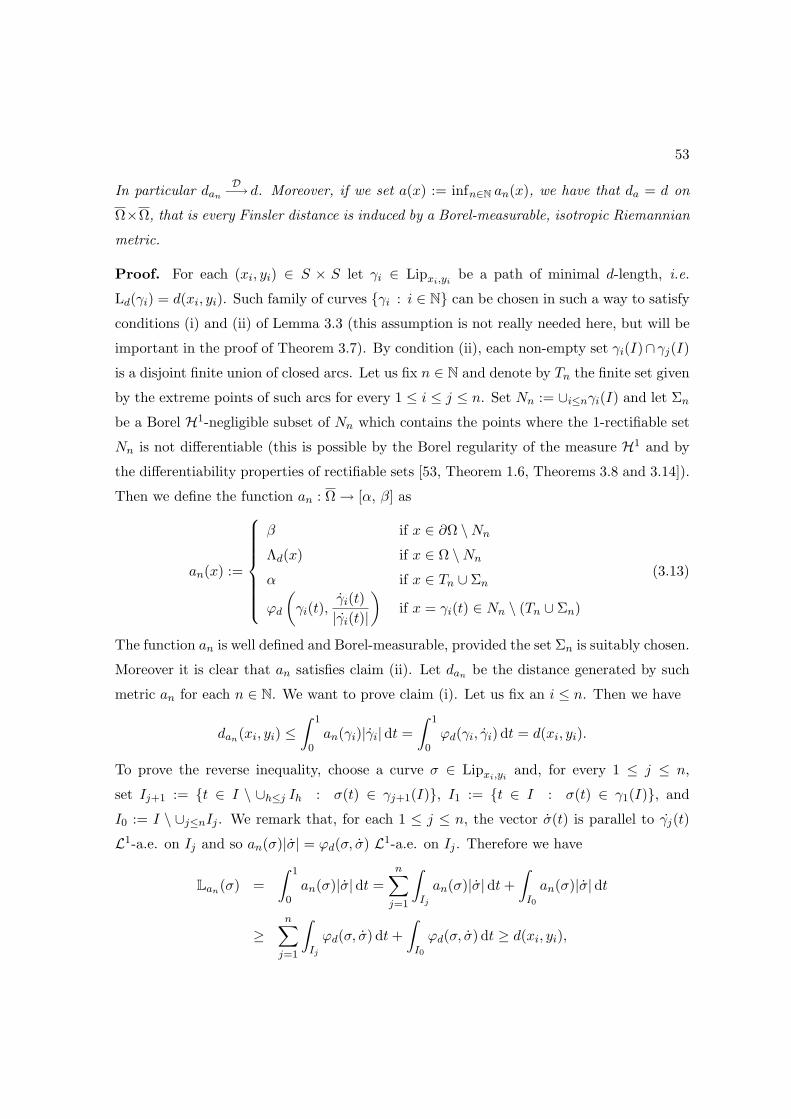
53

In particular dan

D−→ d. Moreover, if we set a(x) := infn∈N an(x), we have that da = d on

Ω×Ω, that is every Finsler distance is induced by a Borel-measurable, isotropic Riemannian

metric.

Proof. For each (xi, yi) ∈ S × S let γi ∈ Lipxi,yibe a path of minimal d-length, i.e.

Ld(γi) = d(xi, yi). Such family of curves γi : i ∈ N can be chosen in such a way to satisfy

conditions (i) and (ii) of Lemma 3.3 (this assumption is not really needed here, but will be

important in the proof of Theorem 3.7). By condition (ii), each non-empty set γi(I)∩γj(I)

is a disjoint finite union of closed arcs. Let us fix n ∈ N and denote by Tn the finite set given

by the extreme points of such arcs for every 1 ≤ i ≤ j ≤ n. Set Nn := ∪i≤nγi(I) and let Σn

be a Borel H1-negligible subset of Nn which contains the points where the 1-rectifiable set

Nn is not differentiable (this is possible by the Borel regularity of the measure H1 and by

the differentiability properties of rectifiable sets [53, Theorem 1.6, Theorems 3.8 and 3.14]).

Then we define the function an : Ω → [α, β] as

an(x) :=

β if x ∈ ∂Ω \Nn

Λd(x) if x ∈ Ω \Nn

α if x ∈ Tn ∪ Σn

ϕd

(γi(t),

γi(t)|γi(t)|

)if x = γi(t) ∈ Nn \ (Tn ∪ Σn)

(3.13)

The function an is well defined and Borel-measurable, provided the set Σn is suitably chosen.

Moreover it is clear that an satisfies claim (ii). Let dan be the distance generated by such

metric an for each n ∈ N. We want to prove claim (i). Let us fix an i ≤ n. Then we have

dan(xi, yi) ≤∫ 1

0an(γi)|γi| dt =

∫ 1

0ϕd(γi, γi) dt = d(xi, yi).

To prove the reverse inequality, choose a curve σ ∈ Lipxi,yiand, for every 1 ≤ j ≤ n,

set Ij+1 := t ∈ I \ ∪h≤j Ih : σ(t) ∈ γj+1(I), I1 := t ∈ I : σ(t) ∈ γ1(I), and

I0 := I \ ∪j≤nIj . We remark that, for each 1 ≤ j ≤ n, the vector σ(t) is parallel to γj(t)

L1-a.e. on Ij and so an(σ)|σ| = ϕd(σ, σ) L1-a.e. on Ij . Therefore we have

Lan(σ) =∫ 1

0an(σ)|σ| dt =

n∑

j=1

∫

Ij

an(σ)|σ| dt +∫

I0

an(σ)|σ| dt

≥n∑

j=1

∫

Ij

ϕd(σ, σ) dt +∫

I0

ϕd(σ, σ) dt ≥ d(xi, yi),

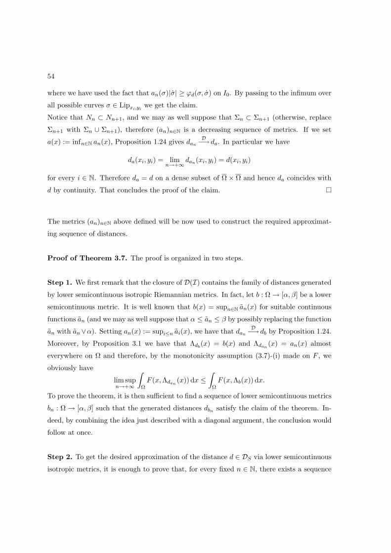
54

where we have used the fact that an(σ)|σ| ≥ ϕd(σ, σ) on I0. By passing to the infimum over

all possible curves σ ∈ Lipxi,yiwe get the claim.

Notice that Nn ⊂ Nn+1, and we may as well suppose that Σn ⊂ Σn+1 (otherwise, replace

Σn+1 with Σn ∪ Σn+1), therefore (an)n∈N is a decreasing sequence of metrics. If we set

a(x) := infn∈N an(x), Proposition 1.24 gives dan

D−→ da. In particular we have

da(xi, yi) = limn→+∞ dan(xi, yi) = d(xi, yi)

for every i ∈ N. Therefore da = d on a dense subset of Ω× Ω and hence da coincides with

d by continuity. That concludes the proof of the claim.

The metrics (an)n∈N above defined will be now used to construct the required approximat-

ing sequence of distances.

Proof of Theorem 3.7. The proof is organized in two steps.

Step 1. We first remark that the closure of D(I) contains the family of distances generated

by lower semicontinuous isotropic Riemannian metrics. In fact, let b : Ω → [α, β] be a lower

semicontinuous metric. It is well known that b(x) = supn∈N an(x) for suitable continuous

functions an (and we may as well suppose that α ≤ an ≤ β by possibly replacing the function

an with an∨α). Setting an(x) := supi≤n ai(x), we have that dan

D−→ db by Proposition 1.24.

Moreover, by Proposition 3.1 we have that Λdb(x) = b(x) and Λdan

(x) = an(x) almost

everywhere on Ω and therefore, by the monotonicity assumption (3.7)-(i) made on F , we

obviously have

lim supn→+∞

∫

ΩF (x,Λdan

(x)) dx ≤∫

ΩF (x,Λb(x)) dx.

To prove the theorem, it is then sufficient to find a sequence of lower semicontinuous metrics

bn : Ω → [α, β] such that the generated distances dbn satisfy the claim of the theorem. In-

deed, by combining the idea just described with a diagonal argument, the conclusion would

follow at once.

Step 2. To get the desired approximation of the distance d ∈ DS via lower semicontinuous

isotropic metrics, it is enough to prove that, for every fixed n ∈ N, there exists a sequence

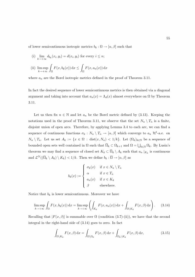
55

of lower semicontinuous isotropic metrics bk : Ω → [α, β] such that

(i) limk→+∞

dbk(xi, yi) = d(xi, yi) for every i ≤ n;

(ii) lim supk→+∞

∫

ΩF (x, bk(x)) dx ≤

∫

ΩF (x, an(x)) dx

where an are the Borel isotropic metrics defined in the proof of Theorem 3.11.

In fact the desired sequence of lower semicontinuous metrics is then obtained via a diagonal

argument and taking into account that an(x) = Λd(x) almost everywhere on Ω by Theorem

3.11.

Let us then fix n ∈ N and let an be the Borel metric defined by (3.13). Keeping the

notations used in the proof of Theorem 3.11, we observe that the set Nn \ Tn is a finite,

disjoint union of open arcs. Therefore, by applying Lemma 3.4 to each arc, we can find a

sequence of continuous functions σk : Nn \ Tn → [α, β] which converge to an H1-a.e. on

Nn \ Tn. Let us set Ak := x ∈ Ω : dist(x,Nn) < 1/k. Let (Ωk)k∈N be a sequence of

bounded open sets well contained in Ω such that Ωk ⊂ Ωk+1 and Ω =⋃

k∈NΩk. By Lusin’s

theorem we may find a sequence of closed set Kk ⊂ Ωk \Ak such that an |Kkis continuous

and LN ((Ωk \Ak) \Kk) < 1/k. Then we define bk : Ω → [α, β] as

bk(x) :=

σk(x) if x ∈ Nn \ Tn

α if x ∈ Tn

an(x) if x ∈ Kk

β elsewhere.

Notice that bk is lower semicontinuous. Moreover we have

lim supk→+∞

∫

ΩF (x, bk(x)) dx = lim sup

k→+∞

(∫

Kk

F (x, an(x)) dx +∫

Ω\Kk

F (x, β) dx

). (3.14)

Recalling that |F (x, β)| is summable over Ω (condition (3.7)-(ii)), we have that the second

integral in the right-hand side of (3.14) goes to zero. In fact∫

Ω\Kk

F (x, β) dx =∫

Ω\Ωk

F (x, β) dx +∫

Ωk\Kk

F (x, β) dx, (3.15)

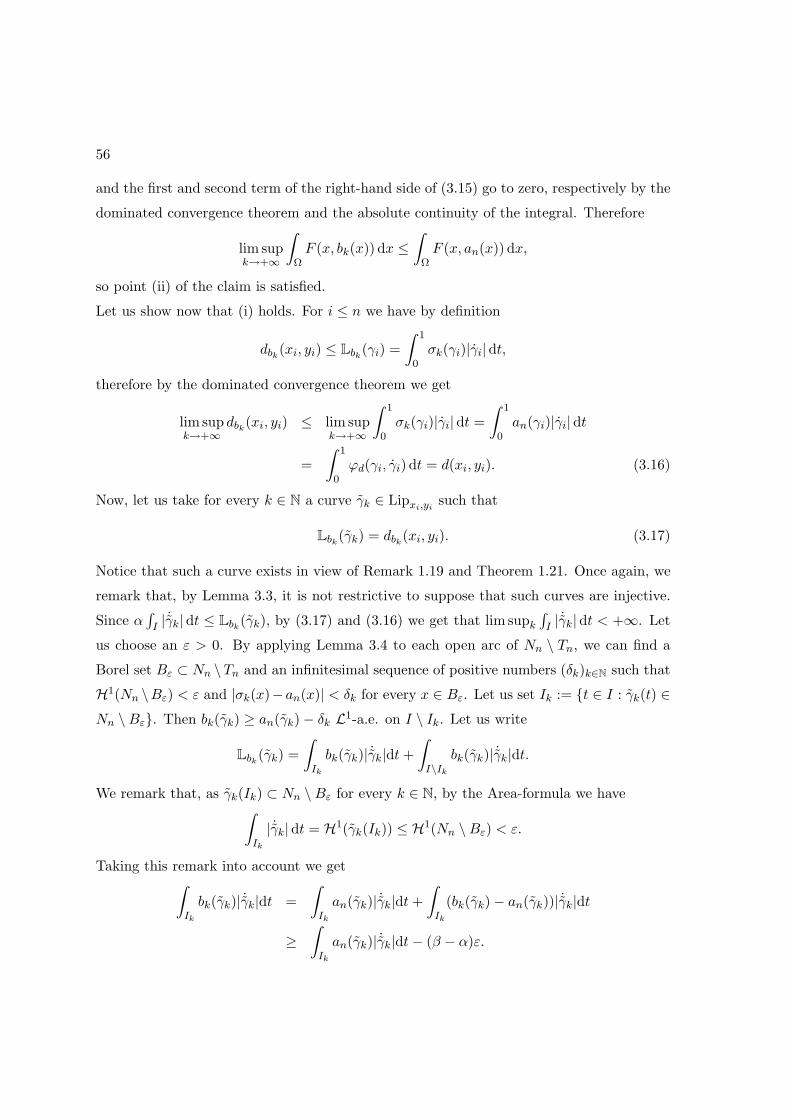
56

and the first and second term of the right-hand side of (3.15) go to zero, respectively by the

dominated convergence theorem and the absolute continuity of the integral. Therefore

lim supk→+∞

∫

ΩF (x, bk(x)) dx ≤

∫

ΩF (x, an(x)) dx,

so point (ii) of the claim is satisfied.

Let us show now that (i) holds. For i ≤ n we have by definition

dbk(xi, yi) ≤ Lbk

(γi) =∫ 1

0σk(γi)|γi| dt,

therefore by the dominated convergence theorem we get

lim supk→+∞

dbk(xi, yi) ≤ lim sup

k→+∞

∫ 1

0σk(γi)|γi| dt =

∫ 1

0an(γi)|γi| dt

=∫ 1

0ϕd(γi, γi) dt = d(xi, yi). (3.16)

Now, let us take for every k ∈ N a curve γk ∈ Lipxi,yisuch that

Lbk(γk) = dbk

(xi, yi). (3.17)

Notice that such a curve exists in view of Remark 1.19 and Theorem 1.21. Once again, we

remark that, by Lemma 3.3, it is not restrictive to suppose that such curves are injective.

Since α∫I | ˙γk| dt ≤ Lbk

(γk), by (3.17) and (3.16) we get that lim supk

∫I | ˙γk| dt < +∞. Let

us choose an ε > 0. By applying Lemma 3.4 to each open arc of Nn \ Tn, we can find a

Borel set Bε ⊂ Nn \Tn and an infinitesimal sequence of positive numbers (δk)k∈N such that

H1(Nn \Bε) < ε and |σk(x)−an(x)| < δk for every x ∈ Bε. Let us set Ik := t ∈ I : γk(t) ∈Nn \Bε. Then bk(γk) ≥ an(γk)− δk L1-a.e. on I \ Ik. Let us write

Lbk(γk) =

∫

Ik

bk(γk)| ˙γk|dt +∫

I\Ik

bk(γk)| ˙γk|dt.

We remark that, as γk(Ik) ⊂ Nn \Bε for every k ∈ N, by the Area-formula we have∫

Ik

| ˙γk|dt = H1(γk(Ik)) ≤ H1(Nn \Bε) < ε.

Taking this remark into account we get∫

Ik

bk(γk)| ˙γk|dt =∫

Ik

an(γk)| ˙γk|dt +∫

Ik

(bk(γk)− an(γk))| ˙γk|dt

≥∫

Ik

an(γk)| ˙γk|dt− (β − α)ε.

57

Then we have

Lbk(γk) ≥

∫ 1

0an(γk)| ˙γk|dt− δk

∫

I\Ik

| ˙γk| dt− (β − α)ε

≥ dan(xi, yi)− δk

∫ 1

0| ˙γk| dt− (β − α)ε

and therefore, as δk

∫ 10 | ˙γk| dt goes to zero when k → +∞, we obtain

lim infk→+∞

dbk(xi, yi) ≥ lim inf

k→+∞Lbk

(γk) ≥ dan(xi, yi)− (β − α)ε.

Since ε was arbitrary, the above inequality coupled with (3.16) gives the claim.

Remark 3.12. It should be noticed that the proof of Theorem 3.7 holds under very general

assumptions on the function F , namely it is sufficient to take an F which is Borel-measurable

and satisfies assumption (ii) of (3.7), and such that the function F (x, ·) is non-decreasing

for LN -a.e. x ∈ Ω. This consideration, together with Remark 3.10, enables us to conclude

that our relaxation result, namely Theorem 3.5, holds under the following milder conditions

on F : Ω× [α, β] → R+:

(i) there exists a sequence of continuous functions Fk : Ω × [α, β] → R+ satisfying con-

ditions (3.7) and such that F (x, ξ) = supk∈N Fk(x, ξ) for LN -a.e. x ∈ Ω, for every

ξ ∈ RN ;

(ii)∫Ω F (x, β) dx < +∞.

58

Chapter 4

Smooth approximation of Finsler

metrics

4.1 Introduction

In this chapter we consider the space Dα of non-symmetric distances defined through (1.11),

where Ω is a connected open subset of RN , and ϕ varies in the family Mα of Borel-

measurable Finsler metrics that satisfy the following bounds for two fixed positive constants

α and β:

α|ξ| ≤ ϕ(x, ξ) ≤ β|ξ| on Ω× RN .

The aim is to show that continuous (smooth) Finsler metrics are dense in Borel ones. More

precisely, we will show that any element of Dα is the uniform limit of a suitable sequence

of distances derived through (1.11) from continuous (smooth) metrics belonging to Mα

(Theorems 4.2 and 4.6). The heavy part of the job corresponds to Theorem 4.2: indeed,

once the density result is proved for continuous metrics, the analogous result for smooth

ones is obtained through a standard mollification argument.

These results can be read as the counterpart of those obtained in Chapter 3, where the

case of symmetric distances was considered, and analogous density theorems for continuous

and smooth Riemannian metrics were obtained (cf. Theorem 3.7 and Remark 3.8). As

a matter of fact, the proofs exploit similar ideas; in particular, the key observation still

corresponds to Lemma 1.22, which allows to replace the uniform convergence of distances

59

60

with a pointwise convergence on a fixed, countable subset of Ω×Ω. On the other hand, new

arguments have to be introduced to overcome the difficulties produced by the non-symmetric

character of distances here considered.

We also wish to underline the content of Theorem 4.3: it amounts to saying that any

geodesic distance d, locally equivalent to the Euclidean one, can be obtained from a convex

Finsler metric through (1.11), a fact which is not trivial at all: notice indeed that the Finsler

metric ϕd(x, ξ), obtained from d by derivation (cf. formula (1.20)), is proved to be convex

in ξ for almost every x only (cf. Theorem 1.8).

The density results obtained for α > 0 are then extended to the case α = 0. The main

difference between the two cases relies on the fact that, while Dα is a closed metric space

when α > 0, this is no longer true when α = 0. This fact is investigated in more detail

in Section 4.4 through suitable, explicit examples. We remark that the family D0 includes

distances for which the local equivalence with the Euclidean one fails to hold somewhere.

The interest for this class of degenerate distances is motivated by the study of Hamilton-

Jacobi equations of eikonal type in the critical case (see [29, 54]).

Last, in Section 4.5 we compare definition (1.11) with a different way of deriving a

distance from a Finsler metric, introduced by De Cecco and Palmieri in [41, 42, 43, 44, 45].

The results there provided will be used in Chapter 5.

4.2 Notation and preliminary results

Throughout this chapter α and β denote two fixed constants with β > α ≥ 0, and Ω an open

connected subset of RN enjoying condition (Ω) of Section 1.3.2. All curves considered in

the sequel will be always assumed to be Lipschitz continuous and parametrized by constant

speed. We denote by Lipx,y the family of curves γ : I → Ω connecting x to y, namely such

that γ(0) = x and γ(1) = y, where I := [0, 1].

Given a measurable function f : I → RN , ‖f‖∞ stands for√∑N

i=0 ‖fi‖2L∞(I), where fi

and ‖fi‖L∞(I) denote the i-th component of f and the L∞-norm of fi respectively.

The closed, convex hull of a subset E of RN will be denoted by co(E). If C is a closed

and convex subset of RN , we will denote by σC the support function of C, namely

σC(ξ) := sup〈ξ, p〉 | p ∈ C .

61

We set

Mα :=ϕ Finsler metric on Ω : α |ξ| ≤ ϕ (x, ξ) ≤ β |ξ| ,

and we denote by Dα = D(Mα) the space of Finsler distances on Ω generated by the metrics

Mα through (1.11), namely

Dα = D(Mα) := dϕ distance on Ω given by (1.11) : ϕ ∈Mα .

In the sequel, we will need the following C1-approximation result, which is just a restatement

of Theorem 1 in [52, Section 6.6].

Theorem 4.1. Suppose γ : I → RN is a (Lispchitz) curve. Then for each ε > 0, there

exists a C1 curve γ : I → RN such that:

L1(t ∈ I : γ(t) 6= γ(t) or γ(t) 6= γ(t) ) ≤ ε.

In addition∥∥γ

∥∥∞ ≤ c ‖γ‖∞

for some constant c depending only on N .

4.3 Approximation results for non-degenerate distances

Throughout this section, α is always assumed to be strictly positive. Our first density result

is then stated as follows:

Theorem 4.2. Let d ∈ Dα. Then there exists a sequence (ϕn)n of continuous and convex

Finlser metrics in Mα such that dϕn

Dα−→ d, where dϕn is the distance associated to ϕn

through (1.11).

The strategy to prove the density result is the same used in Chapter 3: when defining the

approximating sequence ϕn, we only need to control convergence of the induced distances

dϕn to d on a dense subset of Ω×Ω (in view of Lemma 1.22). To this aim, we set S := QN∩Ω.

Obviously S × S is countable and dense in Ω× Ω, so we write S × S := (xi, yi) : i ∈ N.This notation will be adopted in the remainder of this section.

Instead of providing a direct proof to Theorem 4.2, we prefer to break it into intermediate

propositions, which will be proved separately. The first one is an interesting result, which

can be read as a ”dual” formulation of Theorem 3.11.

62

Theorem 4.3. Let d ∈ Dα. Then there exists a decreasing sequence of convex metrics

ψn ∈Mα such that

dψn(xi, yi) = d(xi, yi) for each i ≤ n. (4.1)

Moreover, if we set ψ(x, ξ) := infn ψn(x, ξ) for every (x, ξ) ∈ Ω× RN , then d = dψ, that is

every Finsler distance is induced by a convex Finsler metric.

Proof. For each (xi, yi) ∈ S × S, let γi ∈ Lipxi,yibe a path of minimal d-length, i.e.

Ld(γi) = d(xi, yi), and set Γi := γi ((0, 1)). For every x ∈ Γi, let ξi1(x), ξi

2(x), . . . , ξiN (x)

be an ortonormal basis of RN such that ξi1(γi(t)) = γi(t)/‖γi‖∞ for L1-a.e t ∈ I (recall that

all curves are parametrized by constant speed), and set ai(x) := ϕd(x, ξi1(x)). Such vectors

can be chosen in such a way that the map x → ξij(x) is Borel-measurable on Γi for each

1 ≤ j ≤ N . We define the set-valued map Ci(·) on Ω as follows:

Ci(x) :=

coai(x) ξi

1(x),−β ξi1(x),±βξ2(x), . . . ,±β ξN (x)

if x ∈ Γi

Bα if x ∈ xi, yiBβ otherwise.

Let σi(x, ξ) := σCi(x)(ξ) for every (x, ξ) ∈ Ω× RN . The map σi is easily seen to be Borel-

measurable, and in particular to belong to Mα. The required metrics ψn are now defined

as follows:

ψn(x, ξ) := inf1≤i≤n

σi(x, ξ) for every (x, ξ) ∈ Ω× RN , (4.2)

for each n ∈ N. Obvioulsy, ψn belongs Mα. Let us show now that (4.1) holds. For a fixed

index 1 ≤ i ≤ n we have

dψn(xi, yi) ≤∫ 1

0ψn(γi, γi) dt =

∫ 1

0ϕd(γi, γi) dt = d(xi, yi).

To prove the reverse inequality, choose a curve γ ∈ Lipxi,yiand, for every 1 ≤ j ≤ n−1, set

Ij+1 := t ∈ I\∪h≤j Ih : γ(t) ∈ γj+1(I), I1 := t ∈ I : γ(t) ∈ γ1(I) and I0 := I\∪j≤nIj .

We remark that, for each 1 ≤ j ≤ n, the vector γ(t) is parallel to γj(t) L1-a.e. on Ij and

so ψn(γ, γ) ≥ ϕd(γ, γ) L1-a.e. on Ij (depending on whether the two vectors are equally

oriented or not). Note that this trivially holds for j = 0 too. Therefore we have

Lψn(γ) =∫ 1

0ψn(γ, γ) dt =

n∑

j=0

∫

Ij

ψn(γ, γ) dt ≥n∑

j=0

∫

Ij

ϕd(γ, γ) dt ≥ d(xi, yi),

63

By passing to the infimum over all possible curves γ ∈ Lipxi,yiwe get the claim.

Last, set ψ(x, ξ) := infn ψn(x, ξ) for every (x, ξ) ∈ Ω × RN . By applying Proposition 1.24

(iii), we obtain

dψ(xi, yi) = limn→+∞ dψn(xi, yi) = d(xi, yi) for every i ∈ N,

namely dψ coincide with d on S × S, hence everywhere in Ω× Ω by density.

Next, we prove the following

Proposition 4.4. Let d ∈ Dα. Then, for every n ∈ N and every ε > 0, there exists a lower

semicontinuous, convex metric φε ∈Mα such that

|dφε(xi, yi)− d(xi, yi)| < ε for all i ≤ n. (4.3)

Proof. Note first that, if the functions σi defined in Proof of Theorem 4.3 were continuous

on Γi, a possible choice for φε would be ψn. Hence, the idea is that of modifying the

definition of σi in order to get a continuous function on Γi for each i. We adopt the

notation used in the proof of Theorem 4.3.

Let n ∈ N be fixed, let γi, Γi and ai(x) be defined as above for each i ∈ N, and set

Nn = ∪ni=1Γi. Let us choose λ > 0 and fix an index 1 ≤ i ≤ n. Note that γi is injective

by minimality, hence we can apply Lemma 3.4 to obtain a sequence of continuous functions

aik : Γi → [α, β], k ∈ N, converging pointwise to ai H1-a.e. on Γi as k goes to infinity. Let

γi be the C1-continuous curve obtained by applying Theorem 4.1 with γ := γi and ε := λ.

For every x ∈ Γi, let ξi1(x), ξi

2(x), . . . , ξiN (x) be an orthogonal basis of RN such that:

(i) ξi1(γi(t)) = γi(t)/‖γi‖∞ for L1-a.e t ∈ I;

(ii) |ξij(x)| = 1 for every 2 ≤ j ≤ N .

Such vectors can be chosen in such a way that the map x → ξij(x) is continuous on Γi for

each 1 ≤ j ≤ N . For each k ∈ N, the set-valued map Cik(·) is defined on Ω as follows:

Cik(x) :=

co

aik(x) ξ

i1(x),−β ξ

i1(x),±βξ2(x), . . . ,±β ξN (x)

if x ∈ Γi

Bα if x ∈ xi, yiBβ otherwise.

64

Let σik(x, ξ) :=

(σCi

k(x)(ξ) ∧ β|ξ|)∨ α|ξ| for every (x, ξ) ∈ Ω × RN . The map σi

k is lower

semicontinuous by definition, in particular it belongs to Mα. For each k ∈ N, we define the

metric φk as follows:

φk(x, ξ) := inf1≤i≤n

σik(x, ξ) for every (x, ξ) ∈ Ω× RN . (4.4)

Obviously, φk is lower semicontinuous and belongs Mα. We claim that the following holds:

limk→+∞

|dφk(xi, yi)− d(xi, yi)| ≤ (nβL) λ for all 1 ≤ i ≤ n, (4.5)

where L := max1≤i≤n ‖γi‖∞ This will be enough to conclude: indeed, it is sufficient to take

λ < ε/(nβL) and φε := φk with k suitably large.

Let us then show (4.5). For 1 ≤ i ≤ n we have by definition

dφk(xi, yi) ≤ Lφk

(γi) =∫ 1

0φk(γi, γi) dt.

Let Ji := t ∈ I : γi(t) = γi(t) and recall that, by Theorem 4.1, L1(I \ Ji) ≤ λ. By the

dominated convergence theorem we have

lim supk→+∞

dφk(xi, yi) ≤ lim sup

k→+∞

(∫

Ji

aik(γi)|γi| dt +

∫

I\Ji

β |γi(t)| dt

)

≤∫ 1

0ai(γi)|γi| dt + βLλ = d(xi, yi) + βLλ. (4.6)

Now, set Γ0 := ∪ni=1γi(I \ Ji) and remark that H1(Γ0) ≤ nLλ. Fix an index 1 ≤ i ≤ n. For

each k ∈ N, pick up a curve γk ∈ Lipxi,yisuch that

Lφk(γk) = dφk

(xi, yi). (4.7)

Note that such curves are injective by minimality. Since α∫I | ˙γk| dt ≤ Lφk

(γk), by (4.7) and

(4.6) we get that lim supk

∫I | ˙γk| dt < +∞. Let us choose an ε > 0. By applying Lemma

3.4 to each open arc Γi, we can find a Borel set Bε ⊂ Nn and an infinitesimal sequence

of positive numbers (δk)k∈N such that H1(Nn \ Bε) < ε and |aik(x) − ai(x)| < δk for every

x ∈ Bε, 1 ≤ i ≤ n and k ∈ N. Let us set Ik := t ∈ I : γk(t) ∈ Γ0 ∪ (Nn \ Bε). Then

φk(γk, ˙γk) ≥ ψn(γk, ˙γk)− δk| ˙γk| L1-a.e. on I \ Ik. Let us write

Lφk(γk) =

∫

Ik

φk(γk, ˙γk) dt +∫

I\Ik

φk(γk, ˙γk) dt.

65

We remark that, as γk(Ik) ⊂ Γ0 ∪ (Nn \Bε) for every k ∈ N, by the Area-formula we have∫

Ik

| ˙γk| dt = H1(γk(Ik)) ≤ H1(Nn \Bε) +H1(Γ0) < ε + nLλ.

Taking this remark into account we get∫

Ik

φk(γk, ˙γk)dt =∫

Ik

ψn(γk, ˙γk) dt +∫

Ik

(φk(γk, ˙γk)− ψn(γk, ˙γk)

)dt

≥∫

Ik

ψn(γk, ˙γk) dt− β (ε + nLλ) .

Then we have

Lφk(γk) ≥

∫ 1

0ψn(γk, ˙γk) dt− δk

∫

I\Ik

| ˙γk| dt− β (ε + nLλ)

≥ dψn(xi, yi)− δk

∫ 1

0| ˙γk|dt− β (ε + nLλ)

and therefore, as δk

∫ 10 | ˙γk| dt goes to zero when k → +∞, we obtain

lim infk→+∞

dφk(xi, yi) ≥ lim inf

k→+∞Lφk

(γk) ≥ dψn(xi, yi)− β (ε + nLλ) .

Since ε was arbitrary and dψn(xi, yi) = d(xi, yi), the above inequality coupled with (4.6)

gives the claim.

We are now ready to give the

Proof of Theorem 4.2. First, we claim that, for every ε > 0, there exists a continuous,

convex metric ϕε ∈Mα such that

|dϕε(xi, yi)− d(xi, yi)| < ε for all i ≤ n. (4.8)

Indeed, Proposition 4.4 provides a convex, lower semicontinuous metric φε satisfying (4.8).

By setting φε(x, ξ) := β|ξ| when x ∈ RN \Ω, φε can be extended to RN ×RN . Then Lemma

2.2.3 of [21] easily implies the existence of an increasing sequence (Φn)n of continuous,

convex Finsler metrics on RN such that Φn|Ω×RN ∈ Mα for each n ∈ N and φε(x, ξ) =

supn∈NΦn(x, ξ) in Ω × RN (cf. Proof of [16, Theorem 3.1]). By Proposition 1.24 (i),

the sequence of distances (dΦn)n converges to dφε in Dα, hence (4.8) is proved by setting

ϕε := Φn for n sufficiently large.

66

It is now clear how to conclude: for each n ∈ N, define ϕn := ϕεn with εn := 1/n. The

distances dϕn converge to d pointwise on S×S, which is dense in Ω×Ω, so the claim follows

in view of Lemma 1.22.

Remark 4.5. Note that, by construction, the metrics φn obtained in Proposition 4.4 are

actually defined and continuous in all RN × RN .

The result established in Theorem 4.2 can now be easily improved by requiring the

approximating metrics to be smooth.

Theorem 4.6. Let d ∈ Dα. Then there exists a sequence (ϕn)n of smooth and convex

Finlser metrics in Mα such that dϕn

Dα−→ d.

Proof. Theorem 4.2 provides a sequence (ϕn)n of continuous, convex metrics in Mα

satisfying the claim. Such metrics are actually defined and continuous in RN × RN (cf.

Remark 4.5). Now, take a sequence (ρk)k of convolution kernels and, for each n ∈ N,

let (ρk ∗ ϕn) (x, ξ) :=∫RN ρk(x − y)ϕn(y, ξ) dy. Clearly (ρk ∗ ϕn)k is a sequence of convex,

smooth metrics in Mα, uniformly converging to ϕn on compact subset of Ω×RN . In view

of Proposition 1.24 (ii), the claim follows by setting ϕn := ρk ∗ ϕn for each n ∈ N, with

k := k(n) suitably large.

4.4 The degenerate case

We want to extend the density results obtained in the previous section to the degenerate

case, namely when α = 0. In fact, the analogous of Theorem 4.6 holds.

Theorem 4.7. Let d ∈ D0. Then there exists a sequence (ϕn)n of smooth and convex

Finsler metrics in M0 such that dϕn

D0−→ d.

Proof. Let ϕ ∈ M0 such that d = dϕ. For each k ∈ N, set ϕk(x, ξ) := ϕ(x, ξ) ∨ 1k |ξ| in

Ω × RN . As ϕk ∈ M1/k, we can apply Theorem 4.6 to dϕkfor each k ∈ N, to obtain a

smooth Finsler metric ϕk ∈M1/k such that

|dϕk(xi, yi)− dϕk

(xi, yi)| ≤ 1k

for every i ≤ k.

67

Now the claim easily follows, since the sequence (dϕk)k converges to d in D0 in view of

Remark 1.25.

As already remarked in Section 1.4, the space Dα is closed when α > 0, that is, if (dn)n

is a sequence in Dα converging to d, then d belongs to Dα. Does the same property hold

for α = 0 too?

The point is to show that d is still of geodesic type. When α > 0, this is basically due

to the fact that the corresponding length functionals are equi-coercive, namely Ldn(γ) ≥α

∫ 10 |γ(t)| dt for any curve γ and for each n ∈ N, and this means that any sequence of

curves (γn)n ⊂ Lipx,y such that lim supn Ldn(γn) < +∞ admits (at least) a cluster point

γ ∈ Lipx,y. In particular, for a suitable choice of (γn)n and of γ, that yields

Ld(γ) ≤ lim infn→+∞ Ldn(γn) = lim

n→+∞ dn(x, y) = d(x, y),

which obviously means that d is a geodesic distance. When α = 0, instead, it may hap-

pen that the Euclidean lengths of the curves γn diverge, and two critical phenomena may

basically occur in this case: either the curves go to infinity and disappear in the limit,

or they stay bounded and converge to a non-rectifiable curve (hence, no longer Lipschitz

continuous). In both cases, the limit distance might be not of geodesic type; hence, the

answer to the question previously raised is no: D0 is not closed. Explicit examples of these

possible situations are provided below.

Example. Let Ω := R2, and let us set Γn := (x, y) : x ∈ 0, 1, y ∈ [0, n] ∪ [0, 1]× nfor each n ∈ N, Γ∞ := (x, y) : x ∈ 0, 1, y ∈ [0, +∞] . For each n ∈ N, we define the

metric ϕn on R2 × R2 as follows:

ϕn(x, ξ) :=

14n2 |ξ| if x ∈ Γn and ξ ∈ R2

2|ξ| if x ∈ R2 \ Γn and ξ ∈ R2

Let x0 := (0, 0), y0 := (0, 1), and let dn := dϕn be the distance defined on R2×R2 via (1.11)

for each n ∈ N. Let us notice that dn(x0, y0) = (2n+1)/4n2: in fact, the dn-minimizing path

connecting x0 to y0 is given by the polygonal arc Γn. Up to subsequences, (dn)n converges

(uniformly on compact subset of R2 × R2) to some distance d, by Ascoli-Arzela Theorem.

Now we have that d(x0, y0) = 0, while the d-metric length of any curve connecting x0 to y0

68

is at least 2. To see this, simply notice that ϕd(x, ξ) = 2|ξ| for every x ∈ R2 \ Γ∞. Hence d

is not of geodesic type, though uniform limit of geodesic distances.

Example. Let Ω := (0, 1) × (0, 1) and let q = (1/2, 0), q′ = (1, 1/2). Our example relies

upon the construction provided by Whitney in [73]. In this remarkable paper, Whitney

recursively defines an arc A joining q to q′ of infinite length, and a function f , defined on

Ω and of class C1, whose gradient is null on A, but f(q) = 0 and f(q′) = 1 (in particular,

f is not constant on A).

Such an arc can be represented as the image of a continuous function γ : I → Ω

with γ(0) = q, γ(1) = q′, as explained by the author. Our goal is to define a sequence of

Lipschitz curves uniformly converging to γ. This can be easily done by exploiting Whitney’s

construction. Let us keep the same notation of [73] and assume we are at the n-th step of

the iterative procedure leading to the definition of A, i.e. we have already defined squares

Qi1···it , points qi1···it , q′i1···it and lines Aj1···jt (each ik = 0, 1, 2, 3, each jk = 0, 1, 2, 3, 4) for

t ≤ n. Then, an arc An of finite length, joining q to q′, can be obtained by connecting each

point q′i1···is to qi1···is+1, if is ≤ 2, and q′i1···is−1,3 to qi1···i′s−1by means of a segment, and by

gluing all these segments with all the lines Aj1···jt , t ≤ n. Each arc An may be represented

as the image of a Lipschitz curve γn. Up to a reparametrization (not by constant speed, in

particular), the curves γn uniformly converge to γ, as easily seen.

Let us now denote by ln the Euclidean length of the curve γn, and define the following

sequence (an)n of Riemannian metrics:

an(x) :=

1nln

if x ∈ An

1 if x ∈ Ω \An.

Let dn the distances on Ω×Ω associated to an(x)|ξ| through (1.11). Obviously, dn(q, q′) ≤1/n. Up to subsequences, (dn)n converges to some distance d, by Ascoli-Arzela Theorem,

and obviously d(q, q′) = 0. Notice also that ϕd(x, ξ) = |Df(x)||ξ| for every x ∈ Ω \A. Now,

let us take a curve ξ ∈ Lipq,q′ . We have

Ld(ξ) =∫ 1

0ϕd(ξ(t), ξ(t)) dt ≥

∫ 1

0|Df(ξ(t))| |ξ(t)| dt ≥ f(q′)− f(q) = 1,

so d is not of geodesic type.

69

4.5 Comparison with a different definition of distance

In this section we present a different way to derive a distance from an element ofMα, where

α is now assumed to be a fixed non-negative constant. We recall that a curve γ is said to be

transversal to the set E if H1(γ(I) ∩E) = 0. Then, for each ϕ ∈Mα, we define a function

dϕ on Ω× Ω through the following formula:

dϕ(x, y) := supLN (E)=0

inf

Lϕ(γ) : γ ∈ Lipx,y, γ transversal to E

. (4.9)

Definition (4.9) was introduced by De Cecco and Palmieri in [41, 42, 43, 44, 45] to generalize

the notions of Riemannian and Finsler metric to a Lipschitz manifold, namely a topological

manifold (with countable basis) whose changes of charts are Lipschitz functions. In such

a framework, there was the need of giving an intrinsic definition of length of a curve, i.e.

compatible with the changes of coordinates. Since the latter are Lipschitz continuous, hence

differentiable outside a N -dimensional negligible set, a right notion must be independent

of sets of null measure. Lipschitz manifolds are a generalization of polyhedra, and were

introduced to treat the case of manifolds with singularities, such as vertices, edges, conical

points, even not isolated.

On the other hand, our point of view is different: we are concerned with the singularities

carried by the metric, rather than dealing with those of the manifold. In this setting,

definition (4.9) amounts to ”smoothing” the metric, providing a definition of distance which

is not affected if the metric is bad-behaved on negligible sets.

The purpose of this section is to compare definition (4.9) with definition (1.11) and to

understand the relations between them. The results proved here will be used in Chapter 5.

Throughout the present section, we make the additional assumption that ∂Ω is locally

Lipschitz, i.e. locally coincides with the graph of a Lipschitz continuous function.

Let us denote by Dα := dϕ : ϕ ∈Mα the space of distances generated by the elements

of Mα through (4.9). We have the following result.

Theorem 4.8. Let ϕ ∈ Mα and let dϕ be the distance defined by (4.9). Then there exists

a negligible set F ⊂ Ω such that

dϕ(x, y) = infLϕ(γ) : γ ∈ Lipx,y, γ transversal to F

. (4.10)

70

Moreover, if we set ϕ(x, ξ) := ϕ(x, ξ)χΩ\F (x) + β|ξ|χF (x), we have that dϕ = dϕ, where dϕ

is the distance associated to ϕ through (1.11). In particular, we have that Dα ⊂ Dα.

In order to prove Theorem 4.8, we need a preliminary lemma.

Lemma 4.9. Let γ ∈ Lipx,y with x, y ∈ Ω and let E be a negligible subset of Ω. Then for

every ε > 0 there exists a curve γε ∈ Lipx,y transversal to E and such that ‖γε− γ‖W 1,∞ :=

‖γε − γ‖∞ + ‖γε − γ‖∞ < ε.

Proof. Let γ ∈ Lipx,y and let g(t) ∈ C1(I) be a non negative function such that g(t) = 0 for

t = 0 and t = 1 only (take for example g(t) := sin(πt)). First, let us prove that for LN -a.e.

v ∈ RN the curve γv(t) := γ(t)+vg(t) is transversal to the set E. Set F (t, v) := γ(t)+vg(t)

and let A be the set of points (t, v) ∈ I × RN such that F (t, v) belongs to E. For every

fixed t ∈ (0, 1), the section At := v ∈ RN : (t, v) ∈ A has zero Lebesgue measure in RN ,

therefore A has zero Lebesgue measure in I ×RN . This implies that for every v ∈ RN \N0

the section Av := t ∈ I : (t, v) ∈ A is L1-negligible in I, where N0 is a negligible set

in RN . Therefore, since γv(t) is Lipschitz, for every v ∈ RN \ N0 the set γv(Av) is H1-

negligible in RN , hence the curve γv is transversal to E, as γv(Av) = γv(I) ∩ E. Remark

that ‖γv − γ‖W 1,∞ = |v|‖g‖W 1,∞ .

If γ lies inside Ω, then for |v| small enough the curves γv lie inside Ω. The claim follows

by setting γε := γv with v ∈ RN \N0 and |v| < ε/‖g‖W 1,∞ .

Otherwise, let us assume that the curve γ touches the boundary in a point x0. By

possibly subdividing γ(I) into small subarcs, we may suppose that the curve γ lies in Ω∩B,

where B is a ball centred in x0. This ball can be chosen small enough in such a way that

there exists a cone C := v ∈ Bδ(0) : 〈v, ξ〉 > δ|v| , with δ > 0 and ξ ∈ SN−1 suitably

chosen, such that z + C ⊂ Ω for every z ∈ ∂Ω ∩ B. Remark that, if v ∈ C, the curve γv

lies inside Ω. Therefore, by arguing as above, the claim is achieved by setting γε := γv with

v ∈ C \N0 and |v| < ε/‖g‖W 1,∞ .

Proof of Theorem 4.8: The existence of a negligible set F which satisfies the first assertion

of the claim follows by Proposition 3.5 of [28]. Up to enlarging this set if necessary, we may

as well suppose that F is Borel-measurable.

Set ϕ(x, ξ) := ϕ(x, ξ)χΩ\F (x) + β|ξ|χF (x) and let dϕ be the associated distance defined

according to (1.11). Since Lϕ(γ) = Lϕ(γ) if γ is transversal to F , we obviously have that

71

dϕ ≤ dϕ. We want to prove the reverse inequality. It will be enough to show that for

every γ ∈ Lipx,y and every ε > 0 there exists a curve γε ∈ Lipx,y transversal to F such

that ε + Lϕ(γ) > Lϕ(γε), with x and y arbitrarily chosen in Ω. Then, let γ ∈ Lipx,y and

let A := t ∈ (0, 1) : γ(t) ∈ F . Fix ε > 0 and assume 0 < L1(A) < 1, being the other

cases trivial. Choose an open set J ⊃ A in (0, 1) such that L1(J \ A) < ε. The open set J

is a countable disjoint union of intervals of the form Jk := (ak, bk) with k ∈ N. Applying

Lemma 4.9, we choose, for each k ∈ N, a curve σk : [ak, bk] → Ω transversal to F such that

σk(ak) = γ(ak), σk(bk) = γ(bk) and ‖σk − γ‖W 1,∞(Jk,Ω) < ε/2k. For each n ∈ N let us set:

γn(t) :=

σk(t) if t ∈ [ak, bk] for each k ≤ n

γ(t) otherwise.(4.11)

Let γε be the curve defined by (4.11) with n = +∞. It is easily seen that (γn)n is a Cauchy

sequence in W 1,∞(I,Ω) and converges to γε, which is therefore Lipschitz too. We claim

that γε is the desired curve. Indeed, it connects x and y in Ω and is transversal to F by

construction. Moreover we have:∫

Jk

(ϕ(σk, σk)− ϕ(γ, γ)

)dt ≤ β‖σk‖∞L1(Jk \A) +

∫

Jk∩Aβ(|σk(t)| − |γ(t)|

)dt

< CL1(Jk \A) + βε

2k,

where C is a constant depending only on β and ‖γ‖∞. Therefore

Lϕ(γε)− Lϕ(γ) =+∞∑

k=1

∫

Jk

(ϕ(σk, σk)− ϕ(γ, γ)

)dt < CL1(J \A) + βε < (C + β)ε,

and the claim follows.

Remark 4.10. Let us remark that formula (4.9) is invariant with respect to modifications

of the function ϕ on negligible subsets of Ω. Therefore, since ϕ(x, ξ) = ϕ(x, ξ) for LN -a.e.

x ∈ Ω and every ξ ∈ RN , we also have that dϕ = dϕ = dϕ.

Corollary 4.11. Dα is a proper subset of Dα.

Proof. Let ϕ(x, ξ) be equal to α|ξ| on a segment Γ contained in Ω and β|ξ| elsewhere, and

let d := dϕ be the distance associated to ϕ through (1.11). If d belonged to Dα, by taking

into account Theorem 4.8 and Remark 4.10, we would have d = dψ = dψ for a function

72

ψ ∈ Mα. Proposition 1.15 and the definition of ϕd would imply ψ(x, ξ) ≥ ϕd(x, ξ) = β|ξ|for LN -a.e. x ∈ Ω and every ξ ∈ RN , hence ψ(x, ξ) = β|ξ| LN -a.e. on Ω. Then, by Remark

4.10, we would have d = dψ = βdΩ, which is obviously impossible since d(x, y) = α|x − y|if x and y belong to the segment Γ.

Definitions (1.11) and (4.9) individuate two different ways to derive a distance from

a given ϕ ∈ Mα. In general, we have that dϕ ≤ dϕ, and the inequality may be strict,

as shown by the function ϕ defined in the proof of Corollary 4.11. It seems a difficult

task to characterize the functions ϕ for which equality holds. We therefore restrict to look

for sufficient conditions which entail equivalence between the two definitions. The next

proposition shows that the upper semicontinuity property of the length functional Lϕ plays

a role in this issue.

Proposition 4.12. Let ϕ ∈Mα be such that the length functional Lϕ is upper semicontin-

uous on W 1,∞(I, Ω) with respect to the strong topology. Then dϕ = dϕ.

Proof. Let F be a Borel negligible subset of Ω satisfying (4.10), according to Theorem

4.8. Fix x and y in Ω and let γ ∈ Lipx,y. By applying Lemma 4.9, we find a sequence of

curves (γn)n ⊂ Lipx,y transversal to F which converges to γ in W 1,∞(I, Ω). By the upper

semicontinuity of Lϕ we get

Lϕ(γ) ≥ lim supn→+∞

Lϕ(γn) ≥ dϕ(x, y).

By taking the infimum over all possible curves in Lipx,y we obtain dϕ(x, y) ≥ dϕ(x, y), hence

the claim.

We want to understand under which conditions on the function ϕ the hypothesis of the

previous proposition is satisfied.

Proposition 4.13. Let ϕ ∈ Mα be upper semicontinuous in Ω × RN . Then the length

functional Lϕ is upper semicontinuous on W 1,∞(I, Ω) with respect to the strong topology.

In particular, dϕ = dϕ.

Proof. Let (γn)n be a sequence in W 1,∞(I, Ω) which strongly converges to γ. Using Fatou’s

Lemma and the upper semicontinuity of ϕ we get∫ 1

0ϕ(γ, γ) dt ≥

∫ 1

0lim supn→+∞

ϕ(γn, γn) dt ≥ lim supn→+∞

∫ 1

0ϕ(γn, γn) dt

73

and so the claim.

Remark 4.14. Propositions 4.12 and 4.13 are an adaptation to our setting of similar results

proved in [44].

As a consequence of what seen so far, we obtain the following

Proposition 4.15. Dα is a proper and dense subset of Dα. In particular, it is not closed.

Proof. Proposition 4.13 implies that Dα contains the distances dϕ with ϕ ∈Mα continuous,

so the density follows by Theorem 4.2.

In conclusion, the upper semicontinuity of ϕ is a sufficient condition to entail equivalence

of (1.11) and (4.9) (for instance, the function ϕ defined in the proof of Corollary 4.11 was

lower semicontinuous). On the other hand, it is clear that this condition is far from being

optimal: if the set where ϕ fails to be upper semicontinuous is not too bad, equivalence

between (1.11) and (4.9) still holds. A naive example of this situation is given by a function

ϕ(x, ξ) of the form a(x)|ξ| with a equal to 2 on R× (0, +∞) and to 1 on R× (−∞, 0]. The

proposition that follows generalizes this idea.

Proposition 4.16. Assume that Ω := ∪mi=1Ωi, where the sets Ωi are domains with Lipschitz

boundaries such that Ωi ∩ Ωj = ∂Ωi ∩ ∂Ωj if i 6= j, and every x ∈ Ω belongs to at most

two subdomains Ωi. Let ϕ ∈ Mα and suppose that ϕ is upper semicontinuous in each Ωi.

Moreover, let us assume that for every x ∈ ∪mi=1∂Ωi there exist an index i0 and a real

number ρ(x) > 0 such that x ∈ ∂Ωi0 and ϕ is upper semicontinuous in Ωi0 ∩ Bρ(x). Then

dϕ(x, y) = dϕ(x, y) on Ω× Ω.

Proof. Let F be a Borel negligible subset of Ω satisfying (4.10) in Theorem 4.8. It will be

enough to show that for every γ ∈ Lipx,y and every ε > 0 there exists a curve γε ∈ Lipx,y

transversal to F such that Lϕ(γ) + ε > Lϕ(γε), with x, y ∈ Ω.

Let us then take a curve γ ∈ Lipx,y and fix ε > 0. If γ(I) is contained in Ωi for some

index i, one can apply Lemma 4.9 with Ω := Ωi and conclude by remarking that Lϕ is

upper semicontinuous in W 1,∞(I,Ωi).

Otherwise, there exists a point x ∈ γ(I) ∩ ⋃mi=1 ∂Ωi. Up to subdividing γ(I) into a

finite number of small subarcs, we can assume that γ lies in Br(x)∩Ω, where r < ρ(x) is a

74

sufficiently small radius. The case of x belonging to ∂Ωi for just one index i is easy to deal:

for r small enough Br(x)∩Ω = Br(x)∩Ωi for some index i and ϕ is upper semicontinuous

in Br(x) ∩Ωi by hypothesis, so Lϕ is upper semicontinuous in W 1,∞(I,Br(x) ∩Ω) and the

claim follows by applying Lemma 4.9 again.

Let us then suppose that x belongs to γ(I) ∩ ∂Ωi for two distinct i. Up to reordering

the indexes and to choosing a smaller r, we may suppose x ∈ ∂Ω1 ∩ ∂Ω2, Br(x) ⊂ Ω,

Br(x)∩Ωi = ∅ for each i ≥ 3 and ϕ upper semicontinuous in Ω1 ∩Br(x). Assume also that

r has been chosen so small that there exists a cone C := v ∈ Bδ(0) : 〈v, ξ〉 > δ|v| (for

suitable δ > 0 and ξ ∈ SN−1) such that z + C ⊂ Ω1 for every z ∈ ∂Ω1 ∩Br(x). Arguing as

in the proof of Lemma 4.9, we can take a sequence (vn)n ⊂ C converging to 0 such that the

curves γn(t) := γ(t) + vn sin(πt) are transversal to F and ‖γ − γn‖W 1,∞(I,Ω) ≤ 2|vn|. Let us

set I1 := t ∈ I : γ(t) ∈ Ω1 and I2 := t ∈ I : γ(t) ∈ Ω2 . Notice that, if γ(t) ∈ Ω1, then

γn(t) := γ(t)+vn sin(πt) ∈ Ω1 for every n ∈ N, since the translation by the vector sin(πt)vn

has the effect of moving points on ∂Ω1 inside Ω1. On the other hand, it is clear that if

γ(t) ∈ Ω2 then γn(t) ∈ Ω2 for n big enough. Therefore, by Fatou’s Lemma and taking into

account the upper semicontinuity properties enjoyed by ϕ, we get∫ 1

0ϕ(γ, γ) dt =

∫

I1

ϕ(γ, γ) dt +∫

I2

ϕ(γ, γ) dt ≥∫

I1

lim supn→+∞

ϕ(γn, γn) dt

+∫

I2

lim supn→+∞

ϕ(γn, γn) dt ≥ lim supn→+∞

∫ 1

0ϕ(γn, γn) dt.

The claim follows by setting γε := γn for n big enough.

Chapter 5

Monge solutions for discontinuous

Hamiltonians

5.1 Introduction

We consider the Hamilton-Jacobi equation

H(x,Du) = 0 x ∈ Ω ⊂ RN , (5.1)

where Du is the gradient of the unknown function u : Ω → R and H : Ω × RN → R

is the Hamiltonian. We are concerned with the study of equation (5.1) in the framework

of discontinuous Hamiltonians: indeed, H will be assumed to be only Borel-measurable,

and quasi-convex in the p-variable for every x ∈ Ω. The interest of this issue is easily

motivated by the applications: Hamilton-Jacobi equations with discontinuous ingredients

arise naturally in several models, as, for example, propagation of fronts in non-homogeneous

media, geometric optics in presence of layers, shape-from-shading problems.

One of the main theory concerning Hamilton-Jacobi equations is that of viscosity solu-

tions, developed in the last twenty years. The literature on this subject is wide, as main

reference we recall the books [7], [8] and [63], and the references therein.

With regard to the discontinuous case, measurable fully nonlinear equations of second

order have been studied in [25], however the techniques exploited there are based on the

strong maximum principle so they do not apply to first order equations.

75

76

The first order case has been less studied; we recall, among others (see e.g. [9] and

[59]), [28] and [69]. In the first one Camilli and Siconolfi study equation (5.1) and give a

notion of viscosity solution making use of suitable measure-theoretic devices. They prove

a comparison result, and consequently, when equation (5.1) is coupled with a boundary

datum, they get unicity of the solution and an integral representation formula, generalizing

the one valid for the continuous case. Moreover, such a solution is proven to be the maximal

among Lipschitz subsolutions, in analogy with the classical setting.

In [69], Soravia studies the following Hamilton-Jacobi equation related to optimal control

problems

λu(x) + supa∈A

−f(x, a)Du(x)− h(x, a) = g(x)

where g is only Borel-measurable. The viscosity solutions are defined by taking the lower

and upper semicontinuous envelopes of g following [58]. Uniqueness and stability results

are given.

Both the recalled works start by comparing their definitions with a slightly different

one, given by Newcomb and Su in [66]. The authors studied the equation of eikonal type

H(Du) = n(x) (5.2)

where the discontinuity is in n only, which is assumed to be lower semicontinuous. They in-

troduce the definition of Monge solution, which is shown to be consistent with the viscosity

notion when n is continuous. In this framework they establish the comparison principle for

sub and supersolutions, existence and uniqueness results for (5.2) with Dirichlet boundary

conditions, and a stability result.

In this chapter we want to extend this definition to equations of the more general form

(5.1) and to generalize to this case the above-mentioned results. In order to be more precise

about the type of discontinuities we admit, let us specify that we will deal with Borel-

measurable Hamiltonians H such that Z(x) := p ∈ RN : H(x, p) ≤ 0 is closed and

convex and ∂Z(x) = p ∈ RN : H(x, p) = 0 for every x ∈ Ω. Moreover, we assume

that there exist two positive constants α and β such that Bα(0) ⊂ Z(x) ⊂ Bβ(0) for every

x ∈ Ω.

In analogy with [66], we need to recall that the optical length function relative to the

77

Hamiltonian H is the map S : Ω× Ω → R defined as follows:

S(x, y) := inf∫ 1

0σ(γ(t), γ(t)) dt : γ ∈ Lip

([0, 1], Ω

), γ(0) = x, γ(1) = y

(5.3)

for every x, y ∈ Ω, where σ is the support function of the section Z(x), namely σ(x, ξ) :=

sup 〈−ξ, p〉 : p ∈ Z(x) . Given u ∈ C(Ω), we say that u is a Monge solution (resp. subso-

lution, supersolution) of (5.1) in Ω if for each x0 ∈ Ω there holds

lim infx→x0

u(x)− u(x0) + S(x0, x)|x− x0| = 0 (resp. ≥, ≤).

As it should be clear by the above definition, the properties of Monge sub and super-

solutions strictly depend on those enjoyed by the optical length function S. Note that the

function S is nothing else than the geodesic, non-symmetric distance dσ defined by (1.11).

The results of Chapter 1 (and in particular of Section 1.4) are then specialized to S to carry

on the study of Monge solutions. With this regard, we underline that the lower semicon-

tinuity of the function n in (5.2) is mainly used in [66] to obtain lower semicontinuity of

the length functional Lσ (cf. Remark 1.19), and therefore the existence of an optimal path

for S(x, y), i.e. a path of minimal Lσ-length. This technical difficulty is overcome here by

introducing the metric length of a curve with respect to the non-symmetric distance S (see

(1.1)), which is the relaxed functional of Lσ (in view of Theorem 1.18). The existence of

a minimal path (with respect to the metric S-length) for S(x, y) for all x, y ∈ Ω is then

assured by the results of Chapter 1 (cf. Proposition 1.20). Consequently, under the above-

stated conditions for the Hamiltonian, we obtain a comparison result among Monge sub and

supersolutions of equation (5.1) (Theorem 5.8). This implies moreover that, under certain

compatibility conditions for the boundary data, the Dirichlet problem

H(x,Du) = 0 in Ω

u = g on ∂Ω(5.4)

has a unique Monge solution u, given by Lax formula

u(x) := infy∈∂Ω

S(x, y) + g(y) for all x ∈ Ω, (5.5)

thus recovering a well known result in the case of a continuous Hamiltonian.

In the continuous case, moreover, the function defined by (5.5) is also the maximal

element in the class of Lipschitz subsolutions of (5.4). As already remarked in [66, 69], this

78

is no longer true in general when dealing with Monge solutions of discontinuous Hamilton-

Jacobi equations. However, under mild discontinuous assumptions, the previous maximality

property still holds. This issue will be investigated in a more detailed way in Section 5.5.

As a matter of fact, this will be done by comparing the definition of Monge solution adopted

here with that of viscosity solution introduced by Camilli and Siconolfi in [28]. The main

difference between the two approaches relies upon the definition of optical length function:

while here S is defined by (5.3) through an infimum, the corresponding function LΩ in [28]

is defined through a sup-inf process (cf. Section 5.5 for the definition). The latter has

the effect of rendering the function LΩ independent of modifications of the Hamiltonian

H (and consequently of the support function σ) on negligible subset of Ω with respect to

the x-variable, a property which is necessary if one is interested in keeping the equivalence

(holding in the continuous setting, see [7]) between Lipschitz and viscosity subsolutions

of (5.1). This in particular gives the maximality of the viscosity solution of (5.4) among

Lipschitz subsolutions (cf. [28, Proposition 3.6]). Some problems arise instead when one

deals with sequences of solutions: in [28, Example 7.2], the authors consider a sequence of

continuous Hamilton-Jacobi equations converging to a limit equation for which it is easy

to exhibit a corresponding sequence of viscosity solutions (in the classical sense) uniformly

converging to a function which is not the viscosity solution, in the sense there considered,

of the limit equation (actually, it turns out to be a Monge solution, see Example 5.17). The

main reason of this behavior is that the family of distances that can be obtained through

such a sup-inf process is not closed for the uniform convergence.

On the other hand, the definition of optical length function given here strictly depends on

the pointwise behavior of the Hamiltonian and changing it in the x-variable over negligible

sets does count. Moreover, the class of distances obtained through (5.3) is closed for the

uniform convergence (in fact, it is compact, cf. Theorem 1.21). In particular, with this

approach one can treat optimization problems such as

min∫

Ω|ua − f |2 dx : a : Ω → [α, β] Borel-measurable,

∫

Ωa(x) dx ≤ m

,

where α, β and m are suitable positive constants, f : Ω → R is a given function and ua is

the Monge solution of the following equation, depending on the control a:|Du| = a(x) in Ω

u = 0 on ∂Ω.(5.6)

79

Indeed, the problem can be attacked using the direct method of the Calculus of Variations:

chosen a minimizing sequence (an)n, it is easy to see, using the representation formula

(5.5) and the recalled compactness result, that the corresponding solutions uan converge

uniformly to a function u. To show that u is the Monge solution of problem (5.6) for an

admissible control a one can refer to the results proved in Chapter 3 (specifically, Theorem

3.6 and Theorem 3.11, cf. also Example 5.24).

Throughout all this chapter, Ω will denote a bounded and connected open set of RN

with Lipschitz boundary.

5.2 Monge solutions: definitions and main properties

In this section we study the main properties of Monge sub and supersolutions for the

equation

H(x,Du) = 0 x ∈ Ω ⊂ RN . (5.7)

We will deal with Hamiltonians H satisfying the following set of assumptions (H):

(H1) H : Ω× RN → R is Borel-measurable;

(H2) For every x ∈ Ω the 0-sublevel set

Z(x) := p ∈ RN : H(x, p) ≤ 0 (5.8)

is closed and convex. Moreover ∂Z(x) = p ∈ RN : H(x, p) = 0 for all x ∈ Ω;

(H3) there exist α, β > 0 such that Bα(0) ⊂ Z(x) ⊂ Bβ(0) for every x ∈ Ω.

We recall the definition of optical length function relative to the the Hamiltonian H,

that is the map S : Ω× Ω → R defined by:

S(x, y) := inf∫ 1

0σ(γ(t), γ(t)) dt : γ ∈ Lipx,y

(5.9)

for every x, y ∈ Ω, where σ is the support function of the 0-sublevel set Z(x), namely

σ(x, ξ) := sup 〈−ξ, p〉 : p ∈ Z(x) . (5.10)

Note that, when it will be needed, given an Hamiltonian H, we will respectively denote

by ZH(x), SH(x, y), σH(x, ξ) the corresponding 0-sublevel set (5.8), optical length function

(5.9) and support function (5.10). The definition of Monge solution is given as follows.

80

Definition 5.1. Let u ∈ C(Ω). We say that u is a Monge solution (resp. subsolution,

supersolution) of (5.7) in Ω, if for each x0 ∈ Ω there holds

lim infx→x0

u(x)− u(x0) + S(x0, x)|x− x0| = 0 (resp. ≥, ≤). (5.11)

The general results obtained in Chapter 1 are now applied to derive the main properties

of the optical length function S. Note that S is indeed the non-symmetric distance dϕ

defined in (1.11) with ϕ := σ. We start by studying the regularity of σ in the following

lemma.

Lemma 5.2. If H is an Hamiltonian satisfying (H), then the function σ : Ω × RN → R+

belongs to M and σ(x, ·) is convex on RN for every x ∈ Ω.

Moreover

(i) if H(·, p) is upper semicontinuous on Ω for every p ∈ RN , then σ(·, ξ) is lower semi-

continuous on Ω for every ξ ∈ RN ;

(ii) if H(·, p) is lower semicontinuous on Ω for every p ∈ RN , then σ(·, ξ) is upper semi-

continuous on Ω, for every ξ ∈ RN .

Proof. In order to prove that σ ∈ M, it will be enough to show σ is Borel-measurable,

since all the other properties immediately follow from the definition of σ and assumptions

(H). Let (pi)i be a countable dense subset of RN . By (H2) and (H3), it is easily seen that

σ(x, ξ) = supi∈N

〈−ξ, pi〉 : pi ∈ Z(x) = supi∈N

〈−ξ, pi〉χEi(x) (5.12)

where Ei := x ∈ Ω : H(x, pi) < 0 . Notice that, by assumption (H1), Ei is a Borel

set, hence each function (x, ξ) 7→ 〈−ξ, pi〉χEi(x) is Borel-measurable and the claim follows.

In order to prove (i), we remark that, by assumption (H3), one can replace the functions

〈−ξ, pi〉χEi(x) with (〈−ξ, pi〉∨α|ξ|)χEi

(x) in (5.12) without affecting the equality. Then, as

Ei is open for every i ∈ N, each function x 7→ (〈−ξ, pi〉∨α|ξ|)χEi(x) is lower semicontinuous

for every fixed ξ ∈ RN , and so is σ(·, ξ). The remainder of the claim easily follows by

assumptions (H) and the definition of support function σ.

Remark 5.3. Comparing Lemma 5.2 with Proposition 1.8, we have that the function S is

well-defined. Moreover, it is a non-symmetric geodesic distance such that:

81

(i) α|x− y| ≤ S(x, y) ≤ β|x− y| locally in Ω;

(ii) S is Lipschitz on Ω × Ω, with Lipschitz constant equal to 2β C, where C ≥ 1 is a

Lipschitz constant for ∂Ω.

In particular, by Proposition 1.20, for every x, y ∈ Ω, there exists a curve γ ∈ Lipx,y such

that S(x, y) = LS(γ), where LS(γ) is the length of the curve γ defined according to (1.1)

for the non-symmetric distance S.

We want to show now that the definitions of Monge sub and supersolution are consistent

with those given in the viscosity sense in the classical setting of a continuous Hamiltonian.

Definition 5.4. A function u ∈ C(Ω) is a viscosity subsolution of (5.7) in Ω if

H(x0, q) ≤ 0 for every x0 ∈ Ω and every q ∈ D+u(x0).

Similarly, u ∈ C(Ω) is a viscosity supersolution of (5.7) in Ω if

H(x0, q) ≥ 0 for every x0 ∈ Ω and every q ∈ D−u(x0).

We say that u ∈ C(Ω) is a viscosity solution of (5.7) in Ω if it is both a subsolution and a

supersolution in the viscosity sense. Here we have denoted by D+u(x0) and D−u(x0) the

classical superdifferential and subdifferential of u at x0.

Proposition 5.5. Let H be a continuous Hamiltonian satisfying (H). Then v ∈ C(Ω) is a

Monge supersolution (resp. subsolution) of (5.7) if and only if it is a viscosity supersolution

(resp. subsolution) of (5.7).

Proof. To prove that any viscosity supersolution (resp. subsolution) in C(Ω) is a Monge

supersolution (resp. subsolution), one can argue as in [66].

Conversely, let v ∈ C(Ω) be a Monge supersolution. Let x0 ∈ Ω and q ∈ D−v(x0). By

definition we have

0 ≥ lim infx→x0

v(x)− v(x0) + S(x0, x)|x− x0| ≥ lim inf

x→x0

(〈q, x− x0

|x− x0| 〉+S(x0, x)|x− x0|

). (5.13)

Let (xn)n be a minimizing sequence for the most right-hand side of (5.13). We set

ξn :=xn − x0

|xn − x0| , tn := |xn − x0|.

82

Up to subsequences, we have that ξn → ξ ∈ SN−1. Moreover

lim infn→+∞

S(x0, x0 + tnξn)tn

= lim infn→+∞

S(x0, x0 + tnξ)tn

≥ σ(x0, ξ).

Indeed, the first equality comes from∣∣∣∣S(x0, x0 + tnξn)− S(x0, x0 + tnξ)

tn

∣∣∣∣ ≤ β|ξn − ξ|,

while the second follows by the continuity of H (and therefore of σ by Lemma 5.2) and

Proposition 1.15 (ii). Therefore by (5.13) we obtain

0 ≥ limn→+∞

(〈q, ξn〉+

S(x0, x0 + tnξn)tn

)≥ 〈q, ξ〉+ σ(x0, ξ), (5.14)

that is 〈−ξ, q〉 ≥ σ(x0, ξ) = sup 〈−ξ, p〉 : p ∈ Z(x0) . By Hahn-Banach theorem we get

that H(x0, q) ≥ 0.

Let v ∈ C(Ω) be a Monge subsolution. Let x0 ∈ Ω and q ∈ D+v(x0). We have

0 ≤ lim infx→x0

v(x)− v(x0) + S(x0, x)|x− x0| ≤ lim sup

x→x0

(〈q, x− x0

|x− x0| 〉+S(x0, x)|x− x0|

). (5.15)

If it were H(x0, q) > 0, by Hahn-Banach theorem there would exist a vector ξ ∈ SN−1

such that 〈−ξ, q〉 > sup 〈−ξ, p〉 : p ∈ Z(x0) = σ(x0, ξ). But that is impossible, since, by

taking the sequence xn = x0 + tnξ with tn = 1/n, from inequality (5.15) and Proposition

1.15 (i) we get

0 ≤ 〈q, ξ〉+ lim supn→+∞

S(x0, x0 + tnξ)tn

≤ 〈q, ξ〉+ σ(x0, ξ). (5.16)

In the measurable setting, the following pointwise description of the behavior of Monge sub

and supersolutions holds.

Proposition 5.6. Let v be a Lipschitz function in Ω and H satisfy (H).

(i) If v is a Monge subsolution of (5.7), then it is a Lipschitz subsolution, i.e.

H(x,Dv(x)) ≤ 0 for LN -a.e. x ∈ Ω.

83

(ii) If σ(·, ξ) is lower semicontinuous for every ξ ∈ RN and v is a Monge supersolution of

(5.7), then it is a Lipschitz supersolution, i.e.

H(x, Dv(x)) ≥ 0 for LN -a.e. x ∈ Ω.

In particular, a Monge solution is a Lipschitz solution, i.e. it solves (5.7) almost

everywhere in Ω.

For the proof, the reader may follow word by word that of Proposition 5.5, using Proposi-

tion 1.15 instead of the continuity of the support function σ.

The next proposition says that any Monge subsolution is locally 1-Lipschitz continuous

with respect to the non-symmetric distance S (cf. [66, Lemma 3.1]).

Proposition 5.7. Let H be an Hamiltonian satisfying (H) and u ∈ C(Ω) be a Monge

subsolution of (5.7). Then u is locally Lipschitz in Ω, with Lip(u,Ω) ≤ β. Moreover, for

every x0 ∈ Ω there exists an r > 0, depending only on dist(x0, ∂Ω), α, β, such that

u(x)− u(y) ≤ S(x, y) for every x, y ∈ Br(x0). (5.17)

Proof. First remark that the function u is Lipschitz continuous on Ω. Indeed, by the fact

that u is a Monge subsolution and Remark 5.3, we have that u is a Monge subsolution of

|Dv| = β, hence a (classical) viscosity subsolution. That gives Lip(u,Ω) ≤ β. Now, fix a

point x0 ∈ Ω. Then we can choose an r > 0 small enough so that every optimal path for

S(x, y) with x, y ∈ Br(x0) lies inside Ω. Observe that r is only dependent on dist(x0, ∂Ω), α,

β (cf. Remark 5.3). Fix x, y ∈ Br(x0) and take an optimal path γ ∈ Lipx,y for S(x, y). By

Remark 5.3 the function f(t) := S(x, γ(t)) is Lipschitz continuous. Therefore the function

uγ(t) + f(t) is Lipschitz continuous and we can compute its derivative for L1-a.e. t ∈ I.

We have then

ddt

(uγ + f

)(t) = lim

s→t+

u(γ(s))− u(γ(t)) + S(x, γ(s))− S(x, γ(t))s− t

= |γ(t)| lims→t+

u(γ(s))− u(γ(t)) + S(γ(t), γ(s))|γ(s)− γ(t)| ≥ 0

for L1-a.e. t ∈ I, where we have used the optimality of γ and the definition of Monge

subsolution. By integrating the above inequality we get (5.17), that is the claim.

84

5.3 The comparison result and solvability of the Dirichlet

problem

Our comparison result is stated as follows.

Theorem 5.8 (Comparison Theorem). Let H be an Hamiltonian satisfying (H) and let

u, v ∈ C(Ω) be, respectively, a Monge subsolution and a Monge supersolution of (5.7) in Ω.

If u ≤ v on ∂Ω then u ≤ v in Ω.

The proof is based on the following Lemma (cf. [66, Lemma 3.2]).

Lemma 5.9. Let H and K be two Hamiltonians satisfying (H) and suppose that there exists

a δ ∈ (0, 1) such that

ZK(x) ⊆ δZH(x) ∀x ∈ Ω. (5.18)

Let u ∈ C(Ω) be a Monge subsolution of K(x, Du) = 0 and v ∈ C(Ω) be a Monge superso-

lution of H(x,Dv) = 0. Then u ≤ v on ∂Ω implies u ≤ v in Ω.

Proof. Consider the function

f(x, y) := u(x)− v(y)− SH(x, y)2

ε.

By the continuity of SH we have that f ∈ C(Ω × Ω). Let us argue by contradiction and

suppose that the claim is false. Hence that implies, for an ε > 0 sufficiently small, the

existence of a point (xε, yε) ∈ Ω×Ω where f reaches its maximum. Choose an optimal path

γ ∈ Lipxε,yεand set h(t) :=

(SH(xε, yε) + SH(γ(t), yε)

)/ε. We claim that h(0) ≤ δ < 1. We

may as well suppose that xε 6= yε, otherwise the statement is trivial. The function f(·, yε)

has a local maximum in xε, therefore for t small enough we have f(xε, yε) ≥ f(γ(t), yε), i.e.

u(xε)− u(γ(t)) ≥ 1ε

(SH(xε, yε)2 − SH(γ(t), yε)2

)= h(t)SH(xε, γ(t)).

Since u is a subsolution of K(x,Du) = 0 we can apply (5.17) of Proposition 5.7 and get

SK(xε, γ(t)) ≥ h(t)SH(xε, γ(t)). Assumption (5.18) clearly gives us SK(x, y) ≤ δSH(x, y)

for every x, y ∈ Ω, so we are lead to δSH(xε, γ(t)) ≥ h(t)SH(xε, γ(t)) which clearly gives

the claim.

85

Now f(xε, ·) has a local maximum in yε, so, for y close enough to yε, we have

v(yε)− v(y) ≤ SH(xε, y) + SH(xε, yε)ε

(SH(xε, y)− SH(xε, yε)

)

≤ SH(xε, y) + SH(xε, yε)ε

SH(yε, y) <1 + δ

2SH(yε, y),

that is

v(y)− v(yε) + SH(yε, y)|y − yε| ≥

(1− δ

2

)SH(yε, y)|y − yε| ≥ α

1− δ

2> 0,

which is clearly in contradiction with the fact that v is a Monge supersolution.

Proof of Theorem 5.8: Up to replacing u with u + c and v with v + c for a positive

constant c large enough, we may as well suppose that u is positive on Ω. Let δ ∈ (0, 1)

and Hδ(x, p) := H(x, p/δ). Notice that ZHδ(x) = δZH(x) for every x ∈ Ω, therefore

SHδ= δSH . In particular, this implies that δu is a Monge subsolution of Hδ(x, Dw) = 0.

Moreover, δu ≤ u ≤ v on ∂Ω, so we can apply Lemma 5.9 with K := Hδ to obtain that

δu ≤ v in Ω. The claim then follows by letting δ increase to 1.

We address now our attention to the Dirichlet problem

H(x,Du) = 0 in Ω

u = g on ∂Ω.(5.19)

More precisely, we will prove that the function u given by the Lax formula

u(x) := infy∈∂Ω

S(x, y) + g(y) for x ∈ Ω, (5.20)

is a Monge solution of the Dirichlet problem (5.19) according to the following definition.

Definition 5.10. We will say that a function u ∈ C(Ω) is a Monge solution of the Dirichlet

problem (5.19) if it is a Monge solution of equation H(x,Du) = 0 in Ω and u(x) = g(x) for

each x ∈ ∂Ω.

Our result is the following.

Theorem 5.11 (Solvability of the Dirichlet Problem). Let H be an Hamiltonian

satisfying (H) and assume that the boundary datum g : ∂Ω → R satisfies the compatibility

condition

g(x)− g(y) ≤ S(x, y) for every x, y ∈ ∂Ω. (5.21)

86

The function u given by the Lax formula (5.20) is the unique Monge solution of the Dirichlet

problem (5.19). Moreover, u is the maximal element of the set

SM := v ∈ C(Ω) : v Monge subsolution of (5.7) in Ω, v ≤ g on ∂Ω . (5.22)

The result that follows is preliminary to the proof of the theorem and underlines that

most of the properties enjoyed by the function u defined by (5.20) do not depend in fact on

the compatibility condition (5.21).

Proposition 5.12. Let H be an Hamiltonian satisfying (H) and g : ∂Ω → R be a func-

tion bounded from below. The function u defined by (5.20) is Lipschitz continuous on Ω.

Moreover, u is a Monge solution of (5.7) in Ω.

Proof. As g is bounded from below, u is well defined on Ω by formula (5.20). One can

verify, by definition, that |u(x) − u(y)| ≤ maxS(x, y), S(y, x) on Ω × Ω, therefore u is

Lipschitz continuous on Ω (cf. Remark 5.3), in particular it is of class C(Ω).

To show that u is a Monge subsolution, fix x0 ∈ Ω and an arbitrary sequence (xn)n in

Ω which converges to x0. For every n ∈ N choose a point yn ∈ ∂Ω such that u(xn) ≥S(xn, yn) + g(yn)− o(|x0 − xn|). Then

u(xn) + S(x0, xn) ≥ S(x0, yn) + g(yn)− o(|x− xn|) ≥ u(x0)− o(|x− xn|)

and, by taking the liminf as n goes to +∞ in the above expression, we conclude that u is a

Monge subsolution of (5.7) by the arbitrariness of (xn)n.

Let us prove that u is a Monge supersolution. Fix x0 ∈ Ω and, for n ∈ N big enough, consider

the ball B1/n(x0) ⊂ Ω. Choose an yn ∈ ∂Ω such that u(x0) ≥ S(x0, yn) + g(yn)− 1/n2. Let

γn ∈ Lipx0,ynbe an optimal path for S(x0, yn) and take a point zn ∈ γn(I)∩∂B1/n(x0). By

definition we have that u(zn) ≤ S(zn, yn) + g(yn). Hence, using also the optimality of γn,

we have

u(zn)− u(x0) ≤ S(zn, yn)− S(x0, yn) + 1/n2 = −S(x0, zn) + 1/n2.

This implies

lim infn→+∞

u(zn)− u(x0) + S(x0, zn)|zn − x0| ≤ lim inf

n→+∞1n

= 0,

which obviously implies that u is a Monge supersolution.

87

Proof of Theorem 5.11. Uniqueness in the class C(Ω) is a consequence of the Comparison

Theorem. By Proposition 5.12 we have that the function u defined by (5.20) is Lipschitz

continuous on Ω, in particular of class C(Ω), and is a Monge solution of (5.7) in Ω. We

have, by definition, that u(x) ≤ g(x) for every x ∈ ∂Ω (just choose y = x in formula (5.20)),

while the opposite inequality holds by the compatibility condition (5.21). Hence u = g on

∂Ω, therefore u is the unique solution of class C(Ω) of the Dirichlet problem (5.19). Last,

the maximality of u in the set SM easily follows from Theorem 5.8.

5.4 The stability result

We start this section by introducing a suitable convergence on Hamiltonians under which

we will prove a stability result for Monge solutions.

Definition 5.13. Let (Hn)n, H be Hamiltonians satisfying assumptions (H) and (Sn)n

and S be the relative optical length functions defined according to (5.9). We say that Hn

τ -converges to H and write Hnτ−→H if (Sn)n converges uniformly to S on Ω× Ω.

Remark 5.14. Note that the convergence of the Hamiltonians above defined is equivalent,

by Theorem 1.21, to the Γ-convergence of the length functions (LSn)n to the length functions

LS with respect to the uniform convergence of paths. This, in fact, mainly motivate our

definition.

Since our definition does not give a condition one can check on the sequence (Hn)n, we

will see, in the next proposition, which conditions on the Hamiltonians imply Hnτ−→H.

Proposition 5.15. Let the Hamiltonians H, (Hn)n satisfy (H). Then Hnτ−→H if one of

the following conditions holds:

(i) For each n ∈ N and p ∈ Bβ(0) the function Hn(·, p) is upper semicontinuous on Ω

and (Hn)n converge decreasingly to H on Ω×Bβ(0).

(ii) (Hn)n converges uniformly to H on Ω×Bβ(0).

(iii) (Hn)n converges increasingly to H on Ω×Bβ(0).

88

Proof. By Definition 5.13 the claim will be proved if we show that (Sn)n converge uniformly

to S in Ω× Ω. This easily follows by applying Proposition 1.24 with ϕ := σ and ϕn := σn

for each n ∈ N. Indeed hypothesis (i), (ii), and (iii) respectively imply (i), (ii), and (iii) in

Proposition 1.24 (to obtain (i) we also used Lemma 5.2), and then we can conclude that

the distances associated to σn, i.e. Sn, converge uniformly to the distance associated to σ,

i.e. S.

We are now ready to show our stability result.

Theorem 5.16 (Stability Theorem). Fix α, β > 0 and let us consider an Hamiltonian H

and a sequence of Hamiltonians (Hn)n satisfying assumption (H) for every n ∈ N. Suppose

that:

1. Hnτ−→H as n →∞,

2. un ∈ C(Ω) is a Monge solution of Hn(x,Dun) = 0 in Ω for each n ∈ N;

3. the sequence (un)n converges uniformly to u ∈ C(Ω) on compact subsets of Ω.

Then u is a Monge solution of H(x,Du) = 0 in Ω.

Proof. Fix a point x0 ∈ Ω. By Proposition 5.7, there exists an r > 0 independent of n

such that (5.17) holds for each Sn. Therefore we have

un(x) = infy∈∂Br(x0)

Sn(x, y) + un(y) for every x ∈ Br(x0). (5.23)

By Definition 5.13 (Sn)n converge uniformly to S on Ω×Ω and, by hypothesis 3, un converge

uniformly to u in Br(x0), thus, letting n →∞ in (5.23) we obtain

u(x) = infy∈∂Br(x0)

S(x, y) + u(y) for every x ∈ Br(x0).

So, by Theorem 5.11, u is a Monge solution of H(x, Du) = 0 in Br(x0). The claim then

follows since (5.11) is a local property and x0 ∈ Ω was arbitrary.

We end this section describing an example already studied in [28, Example 7.2]. We

observe that, with our definitions, a stability result holds, while this is not obtained in [28],

89

as stressed by the authors. Note that the difference is in the definition of the optical length

function: indeed, we both consider the same discontinuous Hamiltonian H which is the

pointwise limit of a sequence of continuous ones (Hn)n, but while, using our definition, the

corresponding optical length functions Sn converge uniformly to the optical length function

S corresponding to H, with their definition (cf. also Section 5.5) the sequence (LΩn )n does

not converge to LΩ (note that Sn = LΩn for each n ∈ N as Hn are continuous, cf. Theorem

5.20).

Example 5.17. Let Ω := (0, 1)× (−2, 2) and consider a sequence of continuous functions

an : Ω → R defined by

an(x1, x2) :=

1 if |x2| ≥ 1/n

1/2 + |x2|n/2 otherwise.

The functions an converge increasingly to the function a(x) := χΩ(x)− 1/2χΓ(x) pointwise

on Ω × RN , where Γ is the x1-axis R × 0. Let us define the Hamiltonians Hn(x, p) :=

|p| − an(x) and H(x, p) := |p| − a(x). Obviously, (Hn)n and H satisfy assumptions (H)

with, for instance, α := 1/2 and β := 1. By Proposition 5.15 (i), we immediately have that

Hnτ−→H, therefore the Stability Theorem holds. In particular, if g is a continuous function

on ∂Ω satisfying the compatibility condition (5.21) for H and Hn for each n ∈ N (take, for

instance g(x) := 2|x| for x ∈ ∂Ω), then the Monge solutions un of the Dirichlet problems|Dv| = an(x) in Ω

v = g on ∂Ω

are classical viscosity solutions (as the Hamiltonians Hn are continuous) and converge uni-

formly on Ω× Ω to a function u which is the unique Monge solution of|Dv| = a(x) in Ω

v = g on ∂Ω.

5.5 Pointwise behavior of Monge subsolutions

In this section we will study the pointwise properties enjoyed by the Monge subsolutions

of problem (5.19) and the relation between Monge and Lipschitz subsolutions, in particular

90

we are interested in investigating maximality properties of the function u defined by the

Lax formula (5.20).

We recall that a function v : Ω → R is said to be a Lipschitz subsolution of the Dirichlet

problem (5.19) if v ∈ W 1,∞(Ω), H(x,Dv(x)) ≤ 0 for LN -a.e. x ∈ Ω and v ≤ g on ∂Ω. It

is well known that in the classical context of a continuous Hamiltonian H the function u

defined in (5.20) is the maximum element of the set

SP := v ∈ W 1,∞(Ω) : H(x,Dv(x)) ≤ 0 LN -a.e. in Ω, v ≤ g on ∂Ω

of Lipschitz subsolutions of (5.19). We wonder if this maximality property is maintained

when the Hamiltonian H satisfies the more general hypotheses (H). Indeed, by Proposition

5.12, the function u is a Lipschitz continuous Monge solution of (5.7), therefore is a Lipschitz

subsolution of (5.19), by Proposition 5.6. But in general it is not the maximum element

of SP , not even in the case of a boundary datum g satisfying the compatibility condition

(5.21), as the following example shows.

Example 5.18. Let Ω := (0, 1) × (−1, 1) and let H(x, p) := |p| − a(x), where a(x) :=

2χΩ(x) − χΓ(x) and Γ denotes the x1-axis R × 0. Let v(x1, x2) := 1/2|x2| + 3/2|x1|.Then the inequality H(x,Dv) < 0 holds true for every differentiability point of v in Ω.

Let u be the function given by formula (5.20) with g := v|∂Ω. Observe that g satisfy the

compatibility condition (5.21). Nevertheless, we have u(x1, 0) = S((x1, 0), (0, 0)

)= |x1| <

3/2|x1| = v(x1, 0). Hence, u is not the maximum element of SP .

Therefore we are led to seek for sufficient conditions which guarantee the maximality of

the function u among all Lipschitz subsolution of (5.19).

Let H be an Hamiltonian fulfilling assumptions (H). Following the approach of Camilli and

Siconolfi in [28], we define a slightly different optical length function:

LΩ(x, y) := supLN (E)=0

inf

∫ 1

0σ(γ(t), γ(t)) dt : γ ∈ Lipx,y, γ transversal to E

for every x, y ∈ Ω. We remark that LΩ is nothing else that the distance dσ defined according

to (4.9). The following result holds (cf. [28]).

91

Theorem 5.19. Let H be an Hamiltonian satisfying (H). Assume that g : ∂Ω → R is a

function bounded from below and that S(x, y) = LΩ(x, y) for every x, y ∈ Ω. Then any

Lipschitz subsolution of (5.19) is a Monge subsolution. Moreover, the function u defined by

Lax formula (5.20) is maximal in SP .

The previous theorem gives a first answer to the question raised before. Unfortunately,

the above condition, stated in terms of equality of the optical length functions S and LΩ,

is quite indirect. In order to derive conditions on the Hamiltonian, we now use the results

obtained in Section 4.5. The next theorem will indeed follow quite easily from Proposition

4.16. We remark that our result is more general than those obtained by Newcomb and

Su [66, Theorem 5.4] and by Soravia [69, Theorem 4.7]: indeed, the Hamiltonian H is not

assumed to be piecewise constant in the x-variable near the interface of two contiguous

subdomains.

Theorem 5.20. Assume that Ω := ∪mi=1Ωi, where the sets Ωi are bounded domains with

Lipschitz boundaries such that Ωi ∩Ωj = ∂Ωi ∩ ∂Ωj if i 6= j, and every x ∈ Ω belongs to at

most two subdomains Ωi.

Let H be an Hamiltonian satisfying (H) and lower semicontinuous in Ωi × RN for each i.

Moreover, assume that for every x ∈ ∪mi=1∂Ωi there exist an index i0 and a real number

ρ > 0 such that x ∈ ∂Ωi0 and H is lower semicontinuous in Ωi0 ∩Bρ(x).

Then S(x, y) = LΩ(x, y) for every x, y ∈ Ω. In particular, the claim of Theorem 5.19 holds.

Proof. The claim directly follows by applying Proposition 4.16 with ϕ := σ (as S = dσ

and LΩ = dσ). Since the hypotheses on Ω are satisfied, we only have to check those on

σ. Since σ(x, ·) is convex on RN for every x ∈ Ω, when checking the upper semicontinuity

properties of σ, we can reduce to consider the function σ(·, ξ) for every fixed ξ ∈ RN . Now,

it is easy to prove that σ(·, ξ) is upper semicontinuous on X if H is lower semicontinuous

on X ×RN , being X a subspace of RN and ξ a fixed vector in RN . This argument, applied

with X := Ωi and X := Ωi0 ∩ Bρ(x) with x, io and ρ as in the statement of the theorem,

shows that the assumptions of Proposition 4.16 are fulfilled.

Another question that could be raised is whether the last part of the claim of Theorem

5.11 is still true even when the g does not satisfy the compatibility condition (5.21), that

is we wonder if the function u defined by (5.20) is the maximum element of the set SM for

92

a generic boundary datum. The following example shows that such a maximality property

can not be expected in general.

Example 5.21. Let Ω := (0, 1)× (0, 1) and let H(x, p) := |p| − a(x), K(x, p) := |p| − b(x),

where a(x) := χΩ(x) + χΩ(x) and b(x) := 2χΩ(x). Notice that SK(x, y) = 2|x − y| and

that SH = SK in a suitable neighborhood of every point of Ω. Let g(x) := 2|x| and set, for

every x ∈ Ω,

u(x) := infy∈∂Ω

SH(x, y) + g(y), v(x) := infy∈∂Ω

SK(x, y) + g(y).

Notice that g satisfies the compatibility condition (5.21) with respect to the Hamiltonian

K (but not with respect to H). In particular, that implies v = g on ∂Ω. By Proposition

5.12, u and v are a Monge solutions (in particular, Monge subsolutions) of equation (5.7)

with Hamiltonian H and K respectively. Moreover, since SH = SK locally in Ω and (5.11)

is a local property, we have that v is a Monge subsolution with respect to H too. Let

us show now that u is not greater than v, i.e. that there exists a point x0 ∈ Ω such

that u(x0) < v(x0). To this aim, take x0 := (1/2, 0). Indeed, v(x0) = g(x0) = 1, while

u(x0) ≤ SH(x0, 0) + g(0) = 1/2.

We look for conditions sufficient to guarantee the maximality in SM of the function

u defined in (5.20). A sufficient condition we found is that the optical length function S

defined in (5.9) can be obtained by taking the infimum only over those curves in Lipx,y

which lie in the interior of Ω, possibly except for their endpoints. Note the this condition

is not true in general, as can be easily seen by considering SH in Example 5.21.

Theorem 5.22. Let H be an Hamiltonian satisfying (H). If, for every x, y ∈ Ω,

S(x, y) = inf∫ 1

0σ(γ(t), γ(t)) dt : γ ∈ Lipx,y, γ(t) ∈ Ω for all t ∈ (0, 1)

, (5.24)

then u defined by (5.20) is maximal in SM .

Proof. Let γ be a curve in Lipx,y such that γ(t) ∈ Ω for all t ∈ (0, 1) and let v ∈ SM . For

a fixed positive δ < 1/2, let Γδ := γ ([δ, 1− δ]). The set Γδ is compact and contained in Ω,

93

therefore, by Proposition 5.7, we may find a finite partition δ = t0 < t1 < .. < tm = 1 − δ

such that v(γ(ti))− v(γ(ti+1)) ≤ S(γ(ti), γ(ti+1)) for each i. Therefore

v(γ(δ))− v(γ(1− δ)) ≤m−1∑

i=0

S(γ(ti), γ(ti+1)) ≤m−1∑

i=0

∫ ti+1

ti

σ(γ, γ) dt. (5.25)

By letting δ go to 0 and by taking the infimum of (5.25) over all curves γ ∈ Lipx,y with

γ(t) ∈ Ω for all t ∈ (0, 1), we obtain, in view of assumption (5.24) and the continuity of v,

that

v(x)− v(y) ≤ S(x, y).

In particular the above inequality is true for every y ∈ ∂Ω, therefore, recalling also that

v ≤ g on ∂Ω, we have

v(x) ≤ infy∈∂Ω

S(x, y) + g(y),

which gives the claim.

5.6 Examples

We conclude by discussing some examples. Before going on, we introduce some preliminary

notation. Given a closed subset C of RN , we will denote by dist#(x,C) the signed distance

from the set C, namely the function defined as follows

dist#(x,C) := dist(x,C)− dist(x,RN \ C) for every x ∈ RN .

The dual metric of a Finsler metric ϕ ∈M is the function ϕ∗ defined by

ϕ∗(x, p) := sup 〈p, ξ〉 : ϕ(x, ξ) ≤ 1 for every (x, p) ∈ Ω× RN .

When the metric ϕ is convex, i.e. ϕ(x, ·) is convex for every x ∈ Ω, the following holds (see

[32]):

sup 〈ξ, p〉 : ϕ∗(x, p) ≤ 1 = ϕ(x, ξ) for every (x, ξ) ∈ Ω× RN . (5.26)

Example 5.23. Let us consider the Hamilton-Jacobi equation

H(x,Du) = 0 in Ω, (5.27)

94

where H satisfies assumptions (H), and let S be the associated length function. As S is a

Finsler distance, it is actually the uniform limit of a sequence of distances (dϕn)n, where

ϕn is a continuous Finsler metric belonging M for each n ∈ N (by Theorem 4.2). For each

n ∈ N, let us set

Zn(x) := p ∈ RN : ϕ∗n(x,−p) ≤ 1 for every x ∈ Ω,

and Hn(x, p) := dist#(p, Zn(x)) for every (x, p) ∈ Ω×RN . For each n ∈ N, Hn is continuous,

and it is convex since Zn(x) is a convex set for every x. Moreover, if Sn is the associated

optical length function for each n ∈ N, then Sn = dϕn in view of (5.26) and by definition

of optical length function. Therefore, if g is a boundary datum satisfying the compatibility

condition (5.21) with respect to the length function S, the Monge solution u of

H(x,Dv) = 0 in Ω

v = g on ∂Ω,

is the uniform limit of the unique maximal viscosity solutions un of the problems

Hn(x,Dv) = 0 in Ω

v ≤ g on ∂Ω.

Indeed, by the standard theory of viscosity solutions for continuous Hamiltonians, we know

that un(x) = infy∈∂ΩSn(x, y) + g(y) in Ω, so the claim easily follows in view of Theorem

5.11 and by the uniform convergence of Sn to S.

Example 5.24. In equation (5.27), assume in addition that the Hamiltonina H is such

that the associated optical length function S is symmetric, i.e. S(x, y) = S(y, x) for all

x, y ∈ Ω (this happens, for instance, when H(x, p) is even in p). Then, by Theorem 3.11,

there exists a Borel function a : Ω → [α, β] such that

S(x, y) = inf∫ 1

0a(γ(t))|γ(t)| dt : γ ∈ Lipx,y

for all x, y ∈ Ω.

Therefore, with regard to Monge sub and supersolutions, equation (5.27) is equivalent to

the eikonal equation

|Du| = a(x) in Ω, (5.28)

95

that is, equations (5.27) and (5.28) have the same Monge subsolutions and the same Monge

supersolutions, since they have the same optical length functions. Moreover, by the density

result proven in Section 3.3 (cf. Theorem 3.7), the continuous Hamiltonians Hn of Example

5.23 can be chosen in such a way that Hn(x, p) := |p| − an(x), for a suitable sequence of

Borel-measurable functions an : Ω → [α, β].

Inspired by Example 5.17, we use the same idea to construct an evolutive Hamilton-

Jacobi equation with continuous coefficients, for which standard results of the theory of

Hamilton-Jacobi equations apply. The Cauchy problem obtained by coupling this equation

with a null boundary datum has therefore a unique viscosity solution, which is shown to

tend asymptotically to the Monge solution of a stationary Hamilton-Jacobi equation.

Example 5.25. Let Ω := (0, 1) × (−2, 2) and, for each t > 0, consider the continuous

function at : Ω → R defined by

at(x1, x2) :=

1 if |x2| ≥ 1/t

1/2 + |x2|t/2 otherwise.

Let us define on Ω × (0,+∞) a function a by setting a(x, t) := at(x) for each t > 0 and

x ∈ Ω. We consider the following evolutive Cauchy problem:

∂tv(x, t) + |Dv|(x, t) = a(x, t) in Q := Ω× (0, +∞)

v(x, t) = 0 on ∂Q.(5.29)

Since a(x, t) is continuous, we know, by the standard theory of Hamilton-Jacobi equations

[63], that the above Cauchy problem admits a unique viscosity solution, given by the fol-

lowing formula:

u(x, t) := inf(y,s)∈∂Q

S((x, t), (y, s)) for all (x, t) ∈ Q, (5.30)

where S is the function defined on Q×Q as follows:

S((x, t), (y, s)) := inf∫ t

sa(γ(τ), τ) + H∗(γ(τ)) dτ : γ ∈ Lipy,x([s, t], Ω)

, (5.31)

where Lipy,x([s, t], Ω) denotes the space of curves γ ∈ Lip([s, t], Ω) such that γ(s) = y, γ(t) =

x. When s > t or s = t and x 6= y this family is empty: in that case we agree that

96

S((x, t), (y, s)) = +∞. In the above formula we have denoted by H∗ the Fenchel transform

of H(p) := |p|, namely H∗(ξ) := supp∈RN 〈ξ, p〉 − H(p). Notice that, in this case, H∗

coincides with the indicator function of the closed ball B1(0), i.e. H∗(ξ) is equal to 0 if

|ξ| ≤ 1 and to +∞ otherwise. In particular, S degenerates outside a cone of vertex (x, t),

i.e. S((x, t), (y, s)) = +∞ if t− s < |x− y|.We want to study the asymptotic behavior of the solution u(x, t) of (5.29). Since the

functions at converge pointwise and increasingly on Ω, as t tends to +∞, to the discontinuous

function a∞(x) := χΩ(x) − 1/2χΓ(x) (where we have denoted by Γ the x1-axis R × 0),we expect the asymptotic limit of u(x, t) to solve the stationary Hamilton-Jacobi equation

|Dv| = a∞(x) in Ω.

In fact, we will show that u(x, t) tends asymptotically, uniformly in t, to the Monge solution

of the following Dirichlet problem:|Dv| = a∞(x) in Ω

v = 0 on ∂Ω.(5.32)

To this goal, we first recall (see for instance [63, Theorem 5.2]) that, if in (5.31) the

function a is replaced by a function b : Ω → [α, β], 0 < α < β that does not depend on t,

then, for fixed (x, t) and (y, s) in Q, we have:

S((x, t), (y, s)) ≥ inf∫ T

0b(γ(t))|γ(t)| dt : γ ∈ Lipy,x([0, T ], Ω), T > 0

= db(y, x),

with equality holding if t−s ≥ |y−x|β/α. In particular, by taking into account this remark

and using in (5.31) the fact that a(x, t) ≤ a∞(x) for all (x, t) ∈ Q , one easily obtains that

S((x, t), (y, s)) ≤ 2 diam(Ω) ∨ da∞(x, y) ≤ 2 diam(Ω) for all (x, t) and (y, s) in Q such that

S(x, t), (y, s)) < +∞ (we have denoted by diam(Ω) the diameter of the set Ω). Let us now

fix (x, t) ∈ Q and let γ ∈ Lip([s, t],Ω), 0 ≤ s < t, be a minimizing path of (5.30). Then we

have12(t− s) ≤

∫ t

sa(γ(τ), τ) + H∗(γ(τ)) dτ = u(x, t) ≤ 2 diam(Ω),

that is 0 ≤ t − s ≤ r := 4 diam(Ω). Then, for t > r, any path γ ∈ Lip([s, t],Ω), which is

minimal for (5.30), is such that s ≥ t− r > 0, in particular γ(s) ∈ ∂Ω. Therefore, for t > r,

it is not restrictive to assume that the infimum in (5.30) is taken letting (y, s) vary over

97

the set ∂Ω× [t− r, t] only. In particular, as at−r(z) ≤ a(τ, z) ≤ a∞(z) for every z ∈ Ω and

s ≤ τ ≤ t, we obtain that∫ t

sat−r(γ) + H∗(γ) dτ ≤

∫ t

sa(γ, τ) + H∗(γ) dτ ≤

∫ t

sa∞(γ) + H∗(γ) dτ. (5.33)

Taking the infimum over all possible curves γ joining (y, s) ∈ ∂Ω × [t − r, t] to (x, t) and

letting (y, s) vary in ∂Ω× [t− r, t], by what previously remarked we eventually get

infy∈∂Ω

dat−r(x, y) ≤ u(x, t) ≤ infy∈∂Ω

da∞(x, y).

The claim now follows as at is an increasing sequence of isotropic Riemannian metrics con-

verging pointwise to a∞ on Ω and therefore, by Proposition 1.24, the distance dat uniformly

converges to da∞ on Ω × Ω as t goes to +∞. In particular, this easily implies that u(x, t)

asymptotically converges, uniformly in t, to infy∈∂Ω da∞(x, y), which is the Monge solution

of (5.32) (remark that da∞ is nothing else than the optical length function associated to the

Hamiltonian H(x, p) = |p| − a∞(x)).

The result of the previous example was obtained in a very special case. Nevertheless,

with the same idea, one can obtain an analogous result for Monge solutions of eikonal

equations of the following form:|Dv| = a∞(x) in Ω

v = 0 on ∂Ω,(5.34)

where a∞ : Ω → [α, β] is lower or upper semicontinuous and α and β are, as usual, fixed

positive constants. Indeed, let us assume, for instance, a∞ lower semicontinuous, being

the other case analogous. As well known, it is possible to find an increasing sequence of

continuous functions an : Ω → [α, β], n ∈ N, such that a∞(x) = supn an(x) for all x ∈ Ω.

Let us define on Ω× (0, +∞) a continuous function a by setting a(x, t) := (n+1− t)an(x)+

(t− n)an+1(x) for all x ∈ Ω, t ∈ (n, n + 1] and n ∈ N. Arguing as above, one immediately

gets that the viscosity solution of

∂tv(x, t) + |Dv|(x, t) = a(x, t) in Q := Ω× (0, +∞)

v(x, t) = 0 on ∂Q.

tends asymptotically to the Monge solution of (5.34).

98

Bibliography

[1] E. Acerbi, G. Buttazzo, On the limits of periodic Riemannian metrics. J. Analyse Math. 43

(1983/84), 183-201.

[2] O. Alvarez, Homogenization of Hamilton-Jacobi equations in perforated sets. J. Differential

Equations 159, no. 2 (1999), 543-577.

[3] M. Amar, G. Bellettini, S. Venturini, Integral representation of functionals defined on curves

of W 1,p. Proc. Roy. Soc. Edinburgh Sect. A 128 (1998), 193-217.

[4] M. Amar, E. Vitali, Homogenization of periodic Finsler metrics. J. Convex Anal. 5 (1998),

171-186.

[5] L. Ambrosio, P. Tilli, Selected topics on “Analysis on Metric spaces”. Scuola Normale Superiore

di Pisa, 2000.

[6] D. Bao, S.-S. Chern, Z. Shen, An Introduction to Riemann-Finsler Geometry. Graduate Texts

in Mathematics, 200. Springer-Verlag, New York, 2000.

[7] M. Bardi, I. Capuzzo Dolcetta, Optimal control and viscosity solutions of Hamilton-Jacobi-

Bellman equations. Systems & Control: Foundations & Applications. Birkhuser Boston, Inc.,

Boston, MA, 1997.

[8] G. Barles, Solutions de viscosite des equations de Hamilton-Jacobi. Mathematiques & Appli-

cations, 17, Springer-Verlag, Paris, 1994.

[9] E.N. Barron, R. Jensen, Semicontinuous viscosity solutions for Hamilton-Jacobi equations with

convex Hamiltonians. Comm. Partial Diff. Eq., 49, (1996), 365-397.

[10] J.-D. Benamou, Y. Brenier, A computational fluid mechanics solution to the Monge-

Kantorovich mass transfer problem. Numer. Math. 84(3) (2000), 375-393.

99

100

[11] A. Bensoussan, J.L. Lions, G. Papanicolaou, Asymptotic analysis for periodic structures. Stud-

ies in Mathematics and its Applications, 5. North-Holland Publishing Co., Amsterdam-New

York, 1978.

[12] G. Bouchitte, G. Buttazzo, Characterization of optimal shapes and masses through Monge-

Kantorovich equation. J. Eur. Math. Soc. 3(2) (2001), 139-168.

[13] G. Bouchitte, G. Buttazzo, P. Seppecher, Shape optimization solutions via Monge-Kantorovich

equation. C. R. Acad. Sci. Paris Ser. I Math. 324(10) (1997), 1185-1191.

[14] A. Braides, Almost periodic methods in the theory of homogenization. Appl. Anal. 47 (1992),

259-277.

[15] A. Braides, Γ-convergence for Beginners. Oxford Lecture Series in Mathematics and its Appli-

cations, 22. Oxford University Press, Oxford, 2002.

[16] A. Braides, G. Buttazzo, I. Fragala, Riemannian approximation of Finsler metrics. Asymptotic

Anal. 31 (2) (2001), 177-187.

[17] A. Braides, A. Defranceschi, Homogenization of Multiple Integrals. Oxford Lecture Series in

Mathematics and its Applications, 12. Clarendon Press, Oxford, 1998.

[18] A. Briani, A. Davini, Monge solutions for discontinuous Hamiltonians. Preprint Dipartimento

di Matematica, Universita di Pisa (2003).

[19] D. Burago, Periodic Metrics. Representation theory and dynamical systems. Adv. Soviet. Math.

9 (1992), 205-210.

[20] D. Burago, S. Ivanov, B. Kleiner, On the structure of the stable norm of periodic metrics.

Math. Res. Lett. 4, no. 6 (1997), 791-808.

[21] G. Buttazzo, Semicontinuity, relaxation and integral representation in the calculus of variations.

Pitman Research Notes in Mathematics Series, 207. Longman Scientific, Harlow, 1989.

[22] G. Buttazzo, A. Davini, I. Fragala, F. Macia, Optimal Riemannian distances preventing mass

transfer. J. Reine Angew. Math. (Crelles), to appear.

[23] G. Buttazzo, L. De Pascale, I. Fragala, Topological equivalence of some variational problems

involving distances. Discrete Contin. Dynam. Systems 7(2), (2001), 247-258.

[24] G. Buttazzo, M. Giaquinta, S. Hildebrandt, One-dimensional variational problems. An intro-

duction. Oxford Lecture Series in Mathematics and its Applications, 15. The Clarendon Press,

Oxford University Press, New York, 1998.

101

[25] L. Caffarelli, M. G. Crandall, M. Kocan, A. Swiech, On viscosity solutions of fully nonlinear

equations with measurable ingredients. Comm. Pure Appl. Math. 49, no. 4, (1996), 365-397.

[26] L.A. Caffarelli, M. Feldman, R.J. McCann, Constructing optimal maps for Monge’s transport

problem as a limit of strictly convex costs. J. Amer. Math. Soc. 15(1) (2002), 1-26.

[27] F. Camilli, An Hopf-Lax formula for a class of measurable Hamilton-Jacobi equations. Preprint

(2003).

[28] F. Camilli, A. Siconolfi, Hamilton-Jacobi equations with measurable dependence on the state

variable. Adv. Differential Equations 8, no. 6 (2003), 733-768.

[29] F. Camilli, A. Siconolfi, Homogenization of measurable Eikonal equations. Preprint (2003).

[30] I. Capuzzo Dolcetta, The Hopf solution of Hamilton-Jacobi equations. Elliptic and parabolic

problems (Rolduc/Gaeta, 2001), 343-351, World Sci. Publishing, River Edge, NJ, 2002.

[31] I. Capuzzo Dolcetta, H. Ishii, Hopf formulas for state dependent Hamilton-Jacobi equations,

to appear.

[32] F.H. Clarke, Optimization and Nonsmooth Analysis. John Wiley & Sons, New York, 1983.

[33] M.C. Concordel, Periodic homogenization of Hamilton-Jacobi equations I: additive eigenvalues

and variational formula, Indiana Univ. Math. J. 45 (1996), 1095-1117.

[34] M.C. Concordel, Periodic homogenisation of Hamilton-Jacobi equations. II. Eikonal equations.

Proc. Roy. Soc. Edinburgh Sect. A 127, no. 4 (1997), 665-689.

[35] M.G. Crandall, H. Ishii, P.L. Lions, User’s guide to viscosity solutions of second order partial

differential equations. Bull. Amer. Math. Soc. (N.S.) 27 no. 1 (1992), 1-67.

[36] G. Dal Maso, An introduction to Γ-convergence. Progress in Nonlinear Differential Equations

and their Applications, 8. Birkauser, Boston, 1993.

[37] G. Dal Maso, H. Frankowska, Value functions for Bolza problems with discontinuous La-

grangians and Hamilton-Jacobi inequalities. ESAIM Control Optim. Calc. Var. 5, (2000) 369-

394.

[38] G. Dal Maso, H. Frankowska, Autonomous Integral Functional with Discontinuous Nonconvex

Integrands: Lipschitz Regularity of Minimizers, DuBois-Reymond Necessary Conditions, and

Hamilton-Jacobi Equations. Appl. Math. Optim. 48, no. 1 (2003), 39-66.

102

[39] A. Davini, On the relaxation of a class of functionals defined on Riemannian distances. J.

Convex Anal., to appear.

[40] A. Davini, Smooth approximation of weak Finsler metrics. Preprint Dipartimento di Matem-

atica, Universita di Pisa (2004).

[41] G. De Cecco, G. Palmieri, Distanza intrinseca su una varieta Riemanniana di Lipschitz. Rend.

Sem. Mat. Torino, vol. 46. 2, (1988), 157-170.

[42] G. De Cecco, G. Palmieri, Length of curves on LIP manifolds. Rend. Accad. Naz. Lincei, s. 9,

vol. 1, (1990), 215-221.

[43] G. De Cecco, G. Palmieri, Integral distance on a Lipschitz Riemannian Manifold. Math. Z.

207, (1991), 223-243.

[44] G. De Cecco, G. Palmieri, Distanza intrinseca su una varieta finsleriana di Lipschitz. Rend.

Accad. Naz. Sci. V, XVII, XL, Mem. Mat., 1, (1993), 129-151.

[45] G. De Cecco, G. Palmieri, LIP manifolds: from metric to Finslerian structure. Math. Z. 218(2),

(1995), 223-237.

[46] E. De Giorgi, T. Franzoni, Su un tipo di convergenza variazionale. Atti Accad. Naz. Lincei

Rend. Cl. Sci. Fis. Mat. Natur. 58 (1975), 842-850.

[47] L. De Pascale, A. Pratelli, Regularity properties for Monge transport density and for solutions

to some shape optimization problems. Calc. Var. Partial Differential Equations 14(3) (2002),

249-274.

[48] W. E, A class of homogenization problems in the Calculus of Variations. Commun. Pure Appl.

Math. 44, no. 7 (1991), 733-759.

[49] L.C. Evans, Periodic homogenisation of certain fully nonlinear partial differential equations.

Proc. Roy. Soc. Edinburgh Sect. A 120, no. 3-4 (1992), 245-265.

[50] L.C. Evans, Partial differential equations and Monge-Kantorovich mass transfer, Current de-

velopments in mathematics, 1997 (Cambridge, MA), 65-126, Int. Press, Boston, MA, 1999.

[51] L.C. Evans, W. Gangbo, Differential equations methods for the Monge-Kantorovich mass trans-

fer problem. Mem. Amer. Math. Soc. 137 (1999).

[52] L.C. Evans, R.F. Gariepy, Measure Theory and Fine Properties of Functions. CRC Press, New

York, 1992.

103

[53] K.J. Falconer, The geometry of fractal sets. Cambridge University Press, 1985.

[54] A. Fathi, A. Siconolfi, PDE aspects of Aubry-Mather theory for quasiconvex Hamiltonians,

Calc. Var. Partial Differential Equations, to appear.

[55] M. Feldman, R.J. McCann, Uniqueness and transport density in Monge’s mass transport prob-

lem. Calc. Var. Partial Differential Equations 15 no. 1 (2002), 81-113.

[56] W. Gangbo, R.J. McCann, The geometry of optimal transportation. Acta Math. 177(2) (1996),

113-161.

[57] K. Horie, H. Ishii, Homogenization of Hamilton-Jacobi equations on domains with small scale

periodic structure. Indiana Univ. Math. J. 47, no. 3 (1998), 1011-1058.

[58] H. Ishii, A boundary value problem of the Dirichlet type for Hamilton-Jacobi equations. Ann.

Sc. Norm. Sup. Pisa 16 (IV), (1989), 105-135.

[59] H. Ishii, Hamilton-Jacobi equations with discontinuous Hamiltonians on arbitrary open sets.

Bull. Facul. Sci. & Eng., Chuo Univ., Ser I 28 (1985), 33-77.

[60] L.V. Kantorovich, On the transfer of masses. Dokl. Akad. Nauk. SSSR 37 (1942), 227-229.

[61] L.V. Kantorovich, On a problem of Monge. Uspekhi Mat. Nauk. 3 (1948), 225-226.

[62] S.N. Kruzkov, Generalized solutions of the Hamilton-Jacobi equations of eikonal type. Math.

USSR Sbornik 27 (1975), 406-446.

[63] P.L. Lions, Generalized solutions of Hamilton Jacobi equations. Research Notes in Mathematics,

69. Pitman (Advanced Publishing Program), Boston, Mass.-London, 1982.

[64] P.L. Lions, G. Papanicolaou, S.R.S. Varadhan, Homogenization of Hamilton-Jacobi equations.

Unpublished Preprint (1987).

[65] G. Monge, Memoire sur la theorie des Deblais et des Remblais. Hist. de L’Acad. des Sciences

de Paris (1781).

[66] R.T. Newcomb II, J. Su, Eikonal equations with discontinuities. Differential Integral Equations

8, no. 8, (1995), 1947-1960.

[67] S.T. Rachev, L. Ruschendorf, Mass transportation problems, Vol. I & II. Probability and its

Applications. Springer-Verlag, New York (1998).

104

[68] A. Siconolfi, Metric character of Hamilton-Jacobi equations. Trans. Amer. Math. Soc. 355

(2003), 1987-2009.

[69] P. Soravia, Boundary value problems for Hamilton-Jacobi equations with discontinuous La-

grangian. Indiana Univ. Math. J., 51 no. 2, (2002), 451-477.

[70] P.E. Souganidis, Stochastic homogenization of Hamilton-Jacobi equations and some applica-

tions. Asymptot. Anal. 20, no. 1 (1999) 1-11.

[71] N.S. Trudinger, X.-J. Wang, On the Monge mass transfer problem. Calc. Var. Partial Differ-

ential Equations 13(1) (2001), 19-31.

[72] S. Venturini, Derivation of distance functions in RN . Preprint Dipartimento di Matematica,

Universita di Bologna (1991).

[73] H. Whitney, A function not constant on a connected set of critical points. Duke Mathematical

Journal, no. 1 (1935), 514-517.