Breve storia della modellistica numerica fluido-dinamica

Andrea Doglioli

Sala conferenze ISMAR-CNR, VeneziaMercoledì 14 Luglio 2010

Mappa della Corrente de Golfo di Franklin-Folger,

stampata nel 1769-1770.

Intensità e direzione della corrente superficiale di domani calcolata dal

modello globale (1/12o) HYCOM

I E R I O G G I

http://hdl.loc.gov/loc.gmd/g9112g.ct000753 http://www7320.nrlssc.navy.mil/GLBhycom1-12/glfstr.html

Equazioni per

- Velocità- Temperatura- Salinità

Cos'é un modello numerico dell'oceano?

Un software basato su questo principio

1904 Bjerknes

se si conoscono con sufficente precisione

- lo stato dell'atmosfera a un dato istante (i.e.

le condizioni iniziali ) e

- le leggi che ne governano l'evolversi, allora

possibile prevedere l'evolversi del tempo

Breve storia dei modelli atmosferici ed oceanici

1914 Bjerknes

identificazione de problemi pratici per risolvere numericamente le complicate equazioni

1922 Richardson

si possono introdurre delle approssimazioni fisiche per semplificare il problema matematico e suddividere i conti da svolgere fra un gran numero di persone ben organizzate.

Idea della fabbrica per prevedere il tempo!

Breve storia dei modelli atmosferici ed oceanici

Suddivide l'atmosfera in una griglia di maglia 230 km (in latitudine) per 200 km (in longitudine), trascura la facia equatoriale ed ottine 3 200 colonne verticali attorno alla Terra.In verticale suddivide in tre strati a 4, 7 et 12 km d'altitudine e propone un passo temporale di 3 ore. Per essere più rapido dell'evoluzione reale del tempo, prevede gli servino 64 000 persone

Richardson L. F. (1922) Weather Prediction by Numerical Process

“After so much hard reasoning, may one play with a fantasy? Imagine a large hall like a theatre, except that the circles and galleries go right round through the space usually occupied by the stage. The walls of this chamber are painted to form a map of the globe. The ceiling represents the north polar regions, England is in the gallery, the tropics in the upper circle, Australia on the dress circle and the Antarctic in the pit.

A myriad computers are at work upon the weather of the part of the map where each sits, but each computer attends only to one equation or part of an equation. The work of each region is coordinated by an official of higher rank. Numerous little "night signs" display the instantaneous values so that neighbouring computers can read them. Each number is thus displayed in three adjacent zones so as to maintain communication to the North and South on the map.

From the floor of the pit a tall pillar rises to half the height of the hall. It carries a large pulpit on its top. In this sits the man in charge of the whole theatre; he is surrounded by several assistants and messengers. One of his duties is to maintain a uniform speed of progress in all parts of the globe. In this respect he is like the conductor of an orchestra in which the instruments are slide-rules and calculating machines. But instead of waving a baton he turns a beam of rosy light upon any region that is running ahead of the rest, and a beam of blue light upon those who are behindhand.

[…] ”

Richardson L. F. (1922) Weather Prediction by Numerical Process

“[…]

Four senior clerks in the central pulpit are collecting the future weather as fast as it is being computed, and despatching it by pneumatic carrier to a quiet room. There it will be coded and telephoned to the radio transmitting station. Messengers carry piles of used computing forms down to a storehouse in the cellar.

In a neighbouring building there is a research department, where they invent improvements. But these is much experimenting on a small scale before any change is made in the complex routine of the computing theatre. In a basement an enthusiast is observing eddies in the liquid lining of a huge spinning bowl, but so far the arithmetic proves the better way. In another building are all the usual financial, correspondence and administrative offices. Outside are playing fields, houses, mountains and lakes, for it was thought that those who compute the weather should breathe of it freely.”

1922 Richardson: la fabbrica per prevedere il tempo

Un sistema di calcolo umano (64000 persone) automatico e parallelo con una potenza di calcolo di circa 1 Flops (Floating point operations per second).

«Il sogno di Richardson»

Disegno di François Schuiten (2000)

Una prova con un numero ridotto di personale diede un risultato molto deludente:

- prevista una variazione di pressione circa 145 hPa in 6 ore, un valore

praticamente impossibile (già 20 hPa sono un caso eccezionale)

- in realtà poi la variazione reale fu quasi nulla...

Dove fu l'errore?

Non nella concezione del modello, ma nella poca potenza di calcolo

e nei dati sperimentali, scarsi e poco precisi

Il modello di Richardson, 1922

Oggi esiste una fitta rete di misure meteorologiche

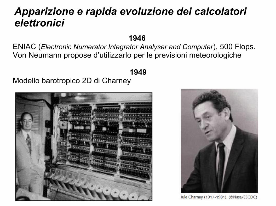
1946 ENIAC (Electronic Numerator Integrator Analyser and Computer), 500 Flops.Von Neumann propose d’utilizzarlo per le previsioni meteorologiche

1949Modello barotropico 2D di Charney

Apparizione e rapida evoluzione dei calcolatori elettronici

Legge di Moore (empirica) : le prestazioni dei computer raddoppiano ogni 18 mesi

25 maggio 2008: Roadrunner, costruito da IBM perl'esercito americano ha raggiunto 1 PetaFlops (1015 Flops)

4 febbraio 2008: Ranger , costruito da AMD per NSF e University of Texas raggiunge 0.5 PetaFlops

1 PetaFlops (1015 Flops)

Nuove architetture

SISD single instruction, single data: processore classico

SIMD single instruction, multiple data: processore vettoriale

MIMD multiple instruction, multiple data: processore parallelo

Memoria condivisaMemoria distribuita (necessita riscrittura

massiva del codice)

Linguaggio di programmazione:prevalentemente in FORTRAN

Ed in campo oceanografico?Semtner, A.J. (1995) Modeling Ocean Circulation. Science, 269, 1397-1385;

"[…] Even though systematic observations began in the 1880s with pioneering observations by Nansen and others (3), the seagoing and theoretical efforts were mainly oriented toward describing large-scale circulation (4), which was often regarded as steady for lack of more detailed information.

It was not until the 1960s, when long-distance tracking of drifting buoys at mid-depth showed currents to be highly variable on quite small spatial scales (5), that oceanographers became aware of the immensity of their task.[...]"

Spirale di Ekman (1902)

XXX X X X

XX

Circolazione de Sverdrup (anni 40) e di Stommel (1947)

Venti Occidentali

Alisei

Richardson, P.L. (1979)Gulf Stream Ring Trajectories, J. Physical Oceanogr., 10, 90-104

Primi modelli oceanici1963 : modello 2DBryan e colleghi del GFDL Geophysical Fluid Dynamics Laboratory (GFDL) (Princeton University & the National Oceanic and Atmospheric Administration);

1969 : modello 3D di Bryan e colleghi.

Bryan, K., and M.D. Cox, The Circulation of the World Ocean: A Numerical Study. Part I, A Homogeneous Model, Journal of Physical Oceanography, 2(4):319-335, 1972.

Modelli oceanici operativi

Modelli oceanici operativi

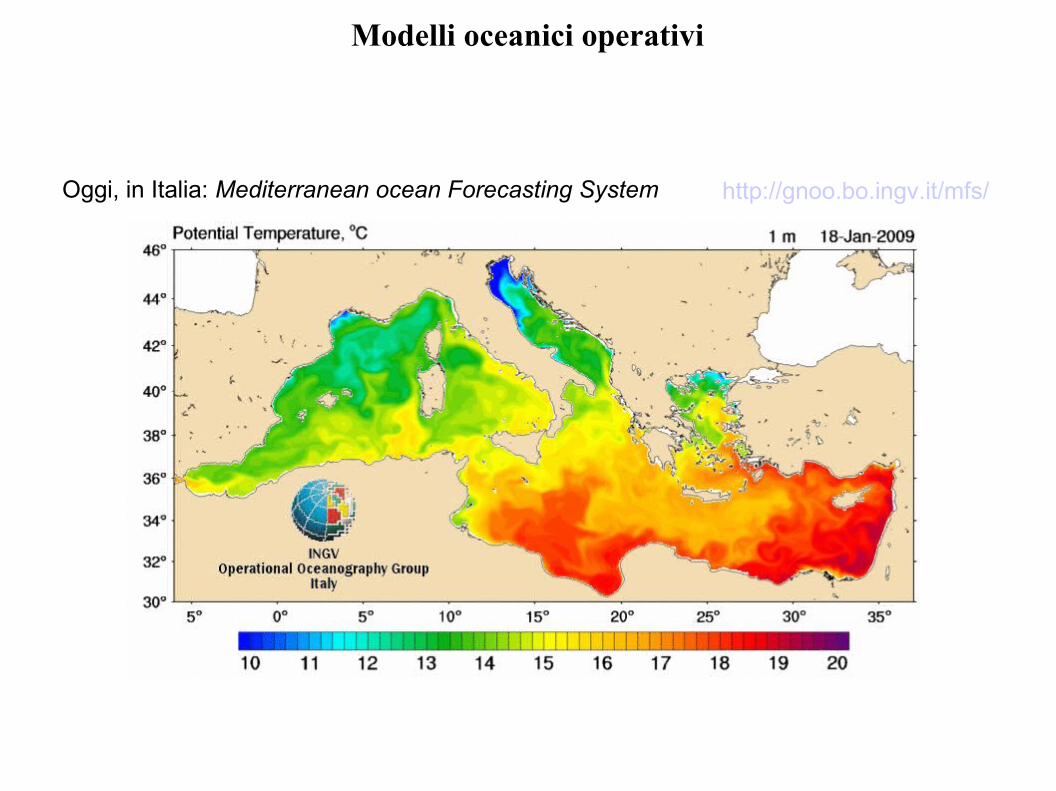
http://gnoo.bo.ingv.it/mfs/Oggi, in Italia: Mediterranean ocean Forecasting System

Modelli oceanici operativi

Modelli oceanici operativi

Era forse « troppo» avanzata

la ricerca di Richardson?!

E quella «dell'entusiasta che studia i vortici»?

Laboratorio del Politecnico di Parigi

- studio dei vortici oceanici in Sud Atlantico

- circolazione e dispersione di inquinanti nelle acque del Promontorio di Portofino

- misura e modellizzazione dei vortici costieri del Golfo del Leone

Esempi di applicazioni di modelli numerici :

Carta delle principali correnti oceanicheanalogie fra i 5 bacini oceanici: lato ovest correnti calde verso i polilato est correnti fredde verso l'equatore

Retroflessione delle Agulhas

e Agulhas Rings del Cape Cauldron

Play

Obbiettivi del progetto

identificare nei dati forniti da un modello i vortici con metodo oggettivo

seguirli nel tempo per capire le loro caratteristiche e gli scambi tra i due oceani

Wavelets Analisys for Time-tracking Eddies in Regional modelS

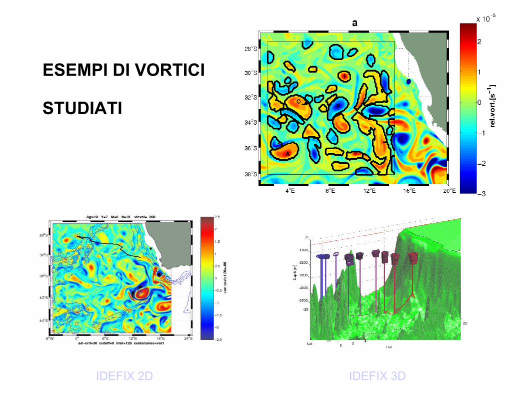
IDEFIX 2D IDEFIX 3D

ESEMPI DI VORTICI

STUDIATI

Cyclone ASTERIX Anticyclone PANORAMIX

45%

3%

10%

9%

30%

1%

52%

6%

4%

12%

16%

7%

Stime degli scambi di masse d'acqua tra Oceano Indiano e Atlantico dovuti ai vortici

Enormi quantità di sale e calore!