andrew hodges- twistor diagram recursion for all gauge-theoretic tree amplitudes

5/11/2018 Andrew Hodges- Twistor diagram recursion for all gauge-theoretic tree amplit...

http://slidepdf.com/reader/full/andrew-hodges-twistor-diagram-recursion-for-all-gauge-theoreti

Twistor diagram recursion for all

gauge-theoretic tree amplitudes

Andrew Hodges

Wadham College, University of Oxford, Oxford OX1 3PN, United Kingdom

March 2005

Abstract: The twistor diagram formalism for scattering amplitudes is introduced,

emphasising its finiteness and conformal symmetry. It is shown how MHVamplitudes are simply represented by twistor diagrams. Then the Britto-Cachazo-

Feng recursion formula is translated into a simple rule for composing twistor

diagrams. It follows that all tree amplitudes in pure gauge-theoretic scattering are

expressed naturally as twistor diagrams. Further implications are briefly discussed.

1. Introduction

Recent work has greatly advanced the study of quantum-field-theoretic amplitudeswith elegant and powerful techniques focused on N=4 supersymmetric gauge field

theory. A frequent comment is that the results turn out to be much simpler than

expected, and that there must be some more fundamental structure yet to be

elucidated. These recent advances have been stimulated by the new formulation of

twistor-string theory by Witten (2003), which indicated twistor space as the correct

setting for this more fundamental structure. Yet twistor geometry has not played a

central role in the exposition of these very recent advances. In particular, the elegant

and powerful recursion relation of Britto, Cachazo and Feng (2004) for buildinggauge-theoretic amplitudes is formulated and proved without any explicit reference

to twistor geometry. Therefore it has been doubted whether twistor theory actually

plays an essential role in the advances being made in gauge-field theory.



The purpose of this note is to point out that in fact, the BCF recursion is intimately

related to twistor theory. It can be naturally and simply stated in terms of the

representation of amplitudes by twistor diagrams. Their recursion formula is

equivalent to a simple graph-theoretic rule for joining twistor diagrams together.

Thus the new recursion relation, far from indicating the possible irrelevance of

twistor geometry, suggests that it may be crucial to further progress.

Twistor diagrams were originally defined by Roger Penrose in about 1970 as the

analogue in twistor space of Feynman diagrams in space-time. The formalism

proposed by Penrose has since then been radically modified, but it retains the most

vital original characteristics. As with Feynman diagrams, twistor diagrams are

integrals built out of simple standard components. They are entirely holomorphic,

using only contour integration. They make explicit where conformal symmetry holdsand where it is broken. They are gauge-invariant. Moreover they are manifestly

finite, the contours all being compact. This finiteness is achieved through a

regularising principle which is essentially twistor-geometric.

As we shall show, Britto, Cachazo and Feng’s formula ensures that all tree

amplitudes are simply expressible as twistor diagrams. However, there is no reason

to suppose that a restriction to tree amplitudes is essential, and we shall add some

remarks on the prospects for representing loop amplitudes. We also point out somewider implications of this reformulation.



2. Twistor Diagrams

As twistor diagrams are not well known, and as the last review (Hodges 1998) is

rather out of date, the formalism will be very briefly introduced. This is best done by

example, rather than by abstract definition. The natural starting-point is supplied by

exhibiting the twistor diagrams for the scattering of four gauge fields. We shall

assume throughout a general knowledge of how the gauge-field amplitudes separate

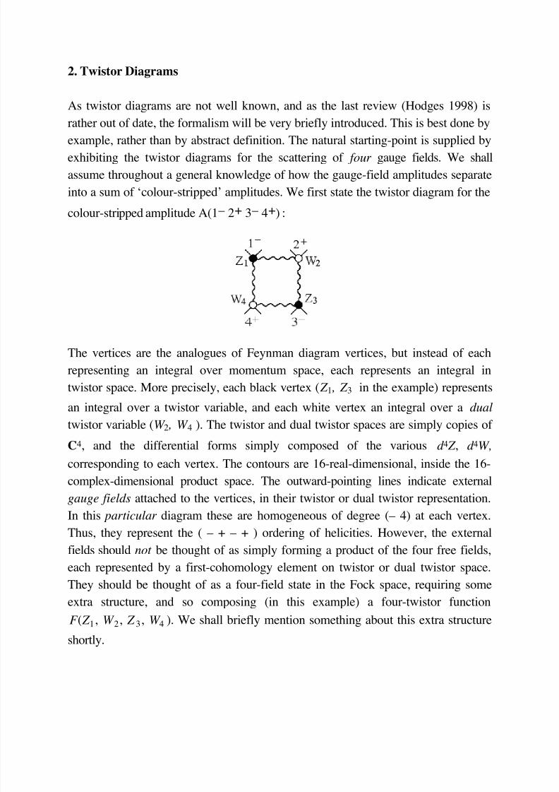
into a sum of ‘colour-stripped’ amplitudes. We first state the twistor diagram for the

colour-stripped amplitude A(1 – 2+ 3 – 4+) :

The vertices are the analogues of Feynman diagram vertices, but instead of each

representing an integral over momentum space, each represents an integral in

twistor space. More precisely, each black vertex ( Z 1, Z 3 in the example) represents

an integral over a twistor variable, and each white vertex an integral over a dual

twistor variable (W 2, W 4 ). The twistor and dual twistor spaces are simply copies of

C4, and the differential forms simply composed of the various d 4 Z , d 4W,

corresponding to each vertex. The contours are 16-real-dimensional, inside the 16-

complex-dimensional product space. The outward-pointing lines indicate external

gauge fields attached to the vertices, in their twistor or dual twistor representation.

In this particular diagram these are homogeneous of degree (– 4) at each vertex.

Thus, they represent the ( – + – + ) ordering of helicities. However, the external

fields should not be thought of as simply forming a product of the four free fields,each represented by a first-cohomology element on twistor or dual twistor space.

They should be thought of as a four-field state in the Fock space, requiring some

extra structure, and so composing (in this example) a four-twistor function

F ( Z 1, W 2, Z 3, W 4 ). We shall briefly mention something about this extra structure

shortly.



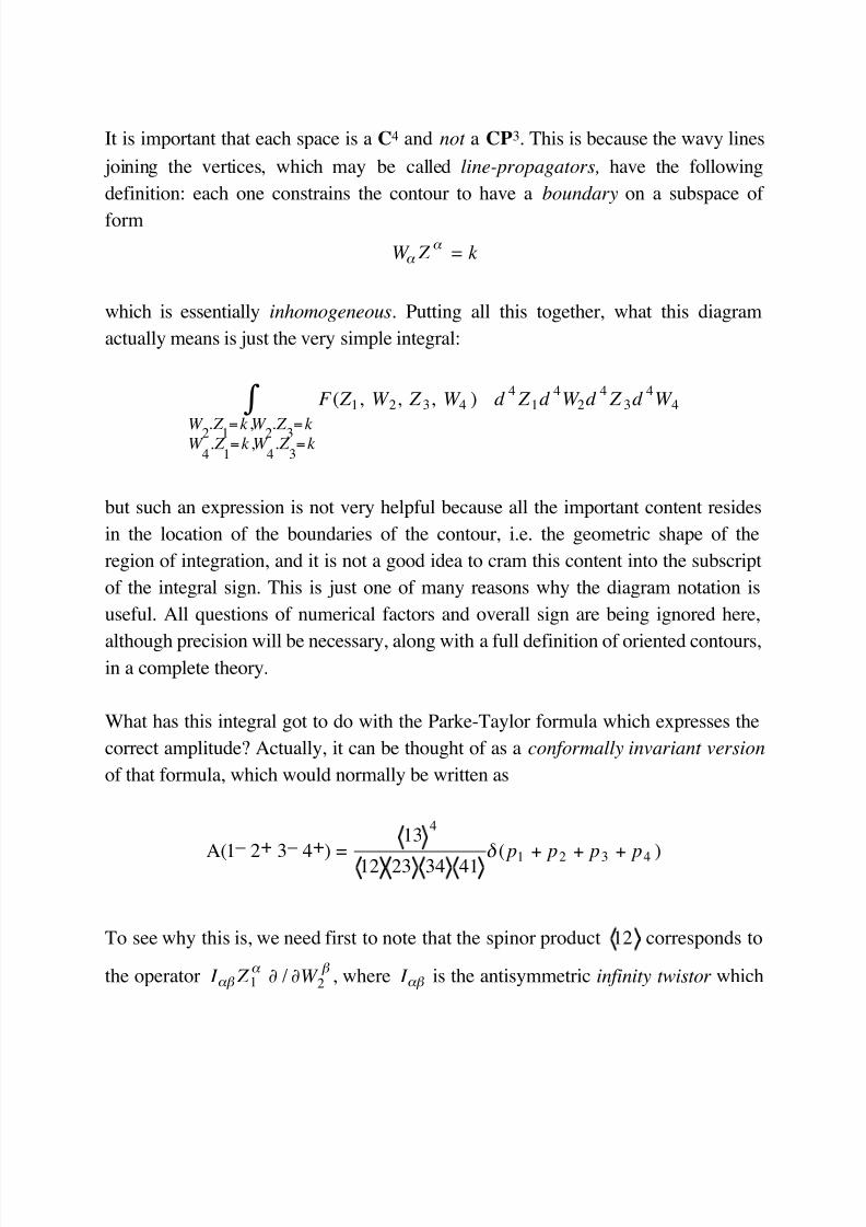
It is important that each space is a C4 and not a CP3. This is because the wavy lines

joining the vertices, which may be called line-propagators, have the following

definition: each one constrains the contour to have a boundary on a subspace of

form

W α Z α

= k

which is essentially inhomogeneous. Putting all this together, what this diagram

actually means is just the very simple integral:

F ( Z 1, W 2, Z 3, W 4 )

W 2. Z 1=k ,W 2. Z 3=k W

4. Z

1=k ,W

4. Z

3=k

∫ d 4 Z 1d

4W 2d

4 Z 3d

4W 4

but such an expression is not very helpful because all the important content resides

in the location of the boundaries of the contour, i.e. the geometric shape of the

region of integration, and it is not a good idea to cram this content into the subscript

of the integral sign. This is just one of many reasons why the diagram notation is

useful. All questions of numerical factors and overall sign are being ignored here,

although precision will be necessary, along with a full definition of oriented contours,in a complete theory.

What has this integral got to do with the Parke-Taylor formula which expresses the

correct amplitude? Actually, it can be thought of as a conformally invariant version

of that formula, which would normally be written as

A(1 –

2+

3 –

4+

) =

134

12 23 34 41 δ ( p1+

p2+

p3+

p4 )

To see why this is, we need first to note that the spinor product 12 corresponds to

the operator I αβ Z 1α

∂ / ∂W 2β

, where I αβ is the antisymmetric infinity twistor which



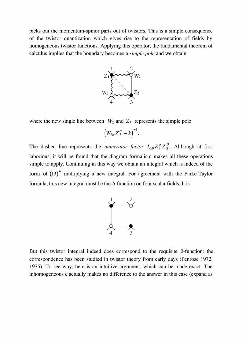
picks out the momentum-spinor parts out of twistors. This is a simple consequence

of the twistor quantization which gives rise to the representation of fields by

homogeneous twistor functions. Applying this operator, the fundamental theorem of

calculus implies that the boundary becomes a simple pole and we obtain

where the new single line between W 2 and Z 3 represents the simple pole

W 2α Z 3α

− k ( )−1

.

The dashed line represents the numerator factor I αβ Z 1α Z 3

β . Although at first

laborious, it will be found that the diagram formalism makes all these operations

simple to apply. Continuing in this way we obtain an integral which is indeed of the

form of 134

multiplying a new integral. For agreement with the Parke-Taylor

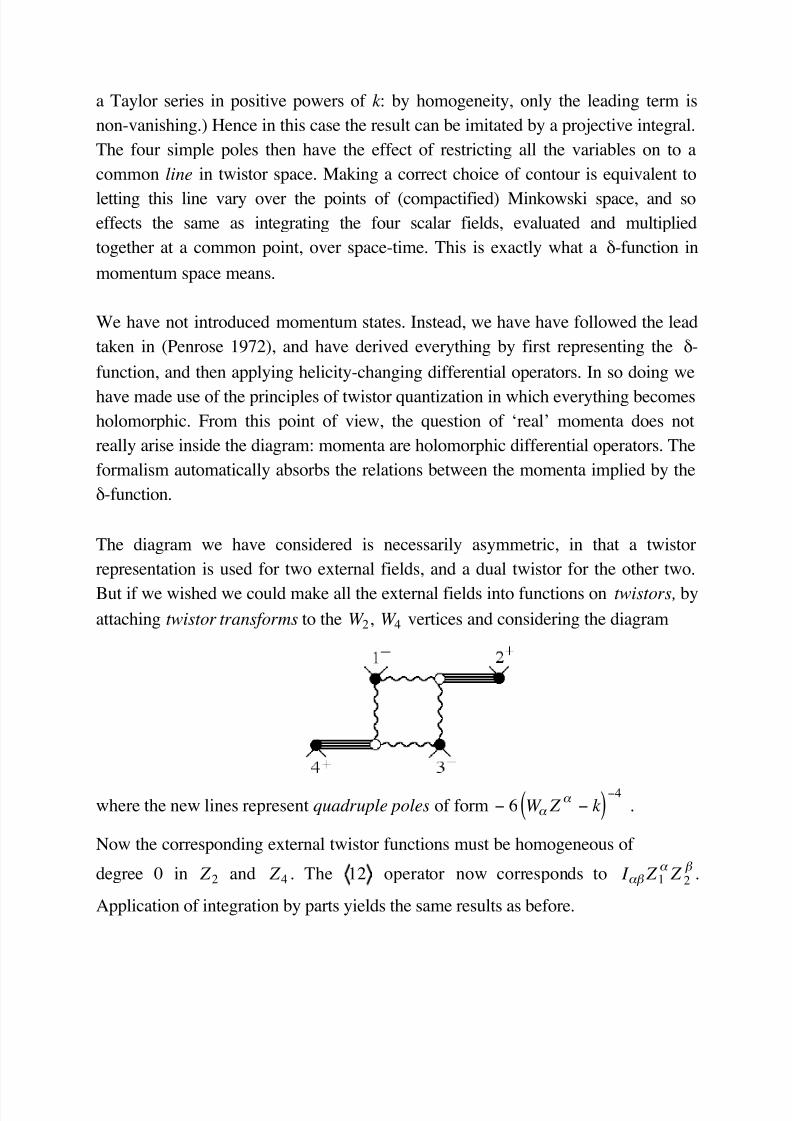
formula, this new integral must be the δ-function on four scalar fields. It is:

But this twistor integral indeed does correspond to the requisite δ-function: the

correspondence has been studied in twistor theory from early days (Penrose 1972,

1975). To see why, here is an intuitive argument, which can be made exact. The

inhomogeneous k actually makes no difference to the answer in this case (expand as



a Taylor series in positive powers of k : by homogeneity, only the leading term is

non-vanishing.) Hence in this case the result can be imitated by a projective integral.

The four simple poles then have the effect of restricting all the variables on to a

common line in twistor space. Making a correct choice of contour is equivalent to

letting this line vary over the points of (compactified) Minkowski space, and so

effects the same as integrating the four scalar fields, evaluated and multiplied

together at a common point, over space-time. This is exactly what a δ-function in

momentum space means.

We have not introduced momentum states. Instead, we have have followed the lead

taken in (Penrose 1972), and have derived everything by first representing the δ-

function, and then applying helicity-changing differential operators. In so doing we

have made use of the principles of twistor quantization in which everything becomes

holomorphic. From this point of view, the question of ‘real’ momenta does not

really arise inside the diagram: momenta are holomorphic differential operators. The

formalism automatically absorbs the relations between the momenta implied by the

δ-function.

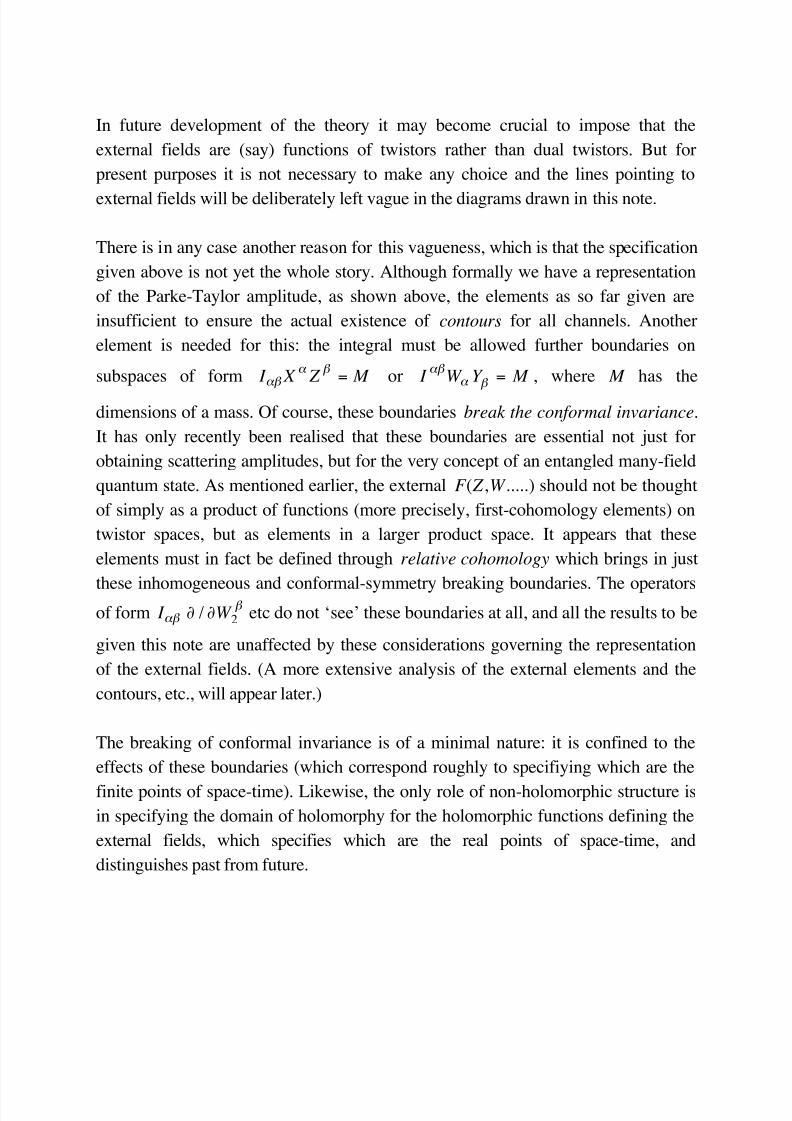
The diagram we have considered is necessarily asymmetric, in that a twistor

representation is used for two external fields, and a dual twistor for the other two.

But if we wished we could make all the external fields into functions on twistors, by

attaching twistor transforms to the W 2, W 4 vertices and considering the diagram

where the new lines represent quadruple poles of form − 6 W α Z α

− k ( )−4

.

Now the corresponding external twistor functions must be homogeneous of

degree 0 in Z 2 and Z 4 . The 12 operator now corresponds to I αβ Z 1α Z 2

β .

Application of integration by parts yields the same results as before.



In future development of the theory it may become crucial to impose that the

external fields are (say) functions of twistors rather than dual twistors. But for

present purposes it is not necessary to make any choice and the lines pointing to

external fields will be deliberately left vague in the diagrams drawn in this note.

There is in any case another reason for this vagueness, which is that the specification

given above is not yet the whole story. Although formally we have a representation

of the Parke-Taylor amplitude, as shown above, the elements as so far given are

insufficient to ensure the actual existence of contours for all channels. Another

element is needed for this: the integral must be allowed further boundaries on

subspaces of form I αβ X α Z

β = M or I

αβ W α Y β = M , where M has the

dimensions of a mass. Of course, these boundaries break the conformal invariance.

It has only recently been realised that these boundaries are essential not just for

obtaining scattering amplitudes, but for the very concept of an entangled many-field

quantum state. As mentioned earlier, the external F ( Z ,W .....) should not be thought

of simply as a product of functions (more precisely, first-cohomology elements) on

twistor spaces, but as elements in a larger product space. It appears that these

elements must in fact be defined through relative cohomology which brings in just

these inhomogeneous and conformal-symmetry breaking boundaries. The operatorsof form I αβ ∂ / ∂W 2

β etc do not ‘see’ these boundaries at all, and all the results to be

given this note are unaffected by these considerations governing the representation

of the external fields. (A more extensive analysis of the external elements and the

contours, etc., will appear later.)

The breaking of conformal invariance is of a minimal nature: it is confined to the

effects of these boundaries (which correspond roughly to specifiying which are the

finite points of space-time). Likewise, the only role of non-holomorphic structure is

in specifying the domain of holomorphy for the holomorphic functions defining the

external fields, which specifies which are the real points of space-time, and

distinguishes past from future.



If evaluation is attempted on finite-normed elements of the Hilbert space (which

momentum states are not!), the collinear singularities of the Parke-Taylor formula

yield a divergent integral. For comparison with experiment the representation in

terms of momentum states is generally the desired one, so there are good reasons

for ignoring this problem for practical purposes. However, the twistor diagram

programme has always set out to compute completely finite amplitudes, consistent

with the fundamentals of quantum mechanics. The inhomogeneous k and M have

the remarkable effect of achieving this finiteness: that is, contours exist for the

inhomogeneous integral given above, which have no analogue in the corresponding

projective integral obtained by letting k and M vanish. It must be stressed that no

change has thereby been made in the Parke-Taylor formula: it is rather that a more

exact and finite specification of its meaning has been made through a new sort of

boundary condition.

The k and M obviously cannot be represented in projective twistor space. This is

how Penrose’s original proposal, which was for projective twistor integrals, has been

most drastically modified (Hodges 1985). Since space-time corresponds to projective

twistor space, we are using a regularisation that is not expressible in space-time: it

uses an extra (but natural) twistor dimension. Possibly, the effect of this

regularisation in loop diagrams will be the same as is obtained by conventional

dimensional regularisation. But this cannot be assumed. The twistor regularisation isessentially different in nature, being completely finite and not requiring any limiting

operations.

There is of course a tantalising possibility here, which deserves exploration, that the

inhomogeneity is intimately related to supersymmetry. It also seems possible that by

generalising this construction, the gauge group could play a direct role in the theory.

However, for the moment we are writing down the simplest possible version of this

kind of inhomogeneous twistor propagator, with a simple scalar and classicalnumber k .

There is a natural value for k , namely exp( – γ ), where γ is Euler’s constant. There

is no obvious value for M , nor is there any reason for it to be either small or large.



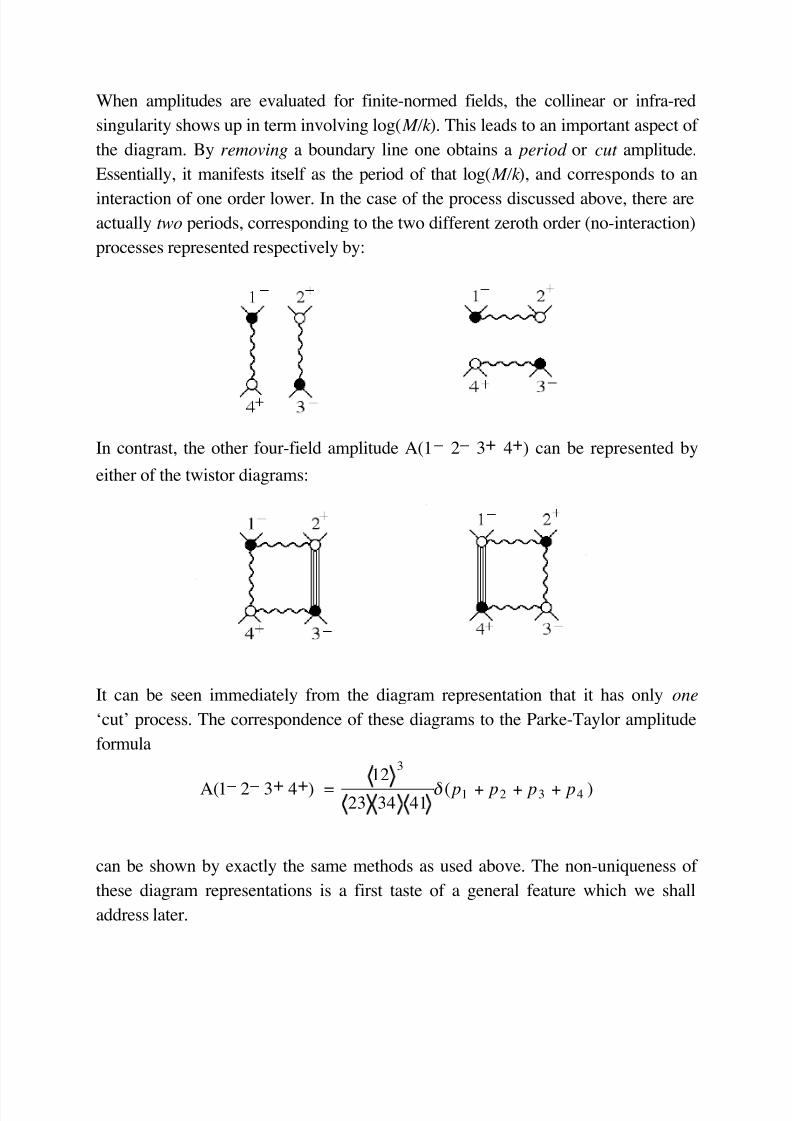
When amplitudes are evaluated for finite-normed fields, the collinear or infra-red

singularity shows up in term involving log( M/k ). This leads to an important aspect of

the diagram. By removing a boundary line one obtains a period or cut amplitude.

Essentially, it manifests itself as the period of that log( M/k ), and corresponds to an

interaction of one order lower. In the case of the process discussed above, there are

actually two periods, corresponding to the two different zeroth order (no-interaction)

processes represented respectively by:

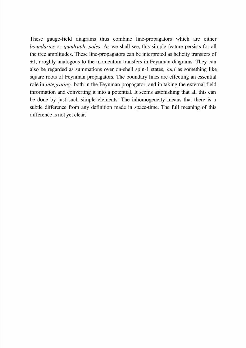
In contrast, the other four-field amplitude A(1 – 2 – 3+ 4+) can be represented by

either of the twistor diagrams:

It can be seen immediately from the diagram representation that it has only one

‘cut’ process. The correspondence of these diagrams to the Parke-Taylor amplitude

formula

A(1 – 2 – 3+ 4+) = 12

3

23 34 41δ ( p1 + p2 + p3 + p4 )

can be shown by exactly the same methods as used above. The non-uniqueness of

these diagram representations is a first taste of a general feature which we shall

address later.


http://slidepdf.com/reader/full/andrew-hodges-twistor-diagram-recursion-for-all-gauge-theoretic

These gauge-field diagrams thus combine line-propagators which are either

boundaries or quadruple poles. As we shall see, this simple feature persists for all

the tree amplitudes. These line-propagators can be interpreted as helicity transfers of

±1, roughly analogous to the momentum transfers in Feynman diagrams. They can

also be regarded as summations over on-shell spin-1 states, and as something like

square roots of Feynman propagators. The boundary lines are effecting an essential

role in integrating: both in the Feynman propagator, and in taking the external field

information and converting it into a potential. It seems astonishing that all this can

be done by just such simple elements. The inhomogeneity means that there is a

subtle difference from any definition made in space-time. The full meaning of this

difference is not yet clear.



3. Delta-function formulas for higher order diagrams

We now wish to obtain diagrams for higher-order processes, proceeding by analogy

with the discussion of four-field processes. We must first have suitable

representations of the delta-function for any number of scalar fields. Then we can

apply helicity-changing operations to obtain corresponding results for gauge-fields.

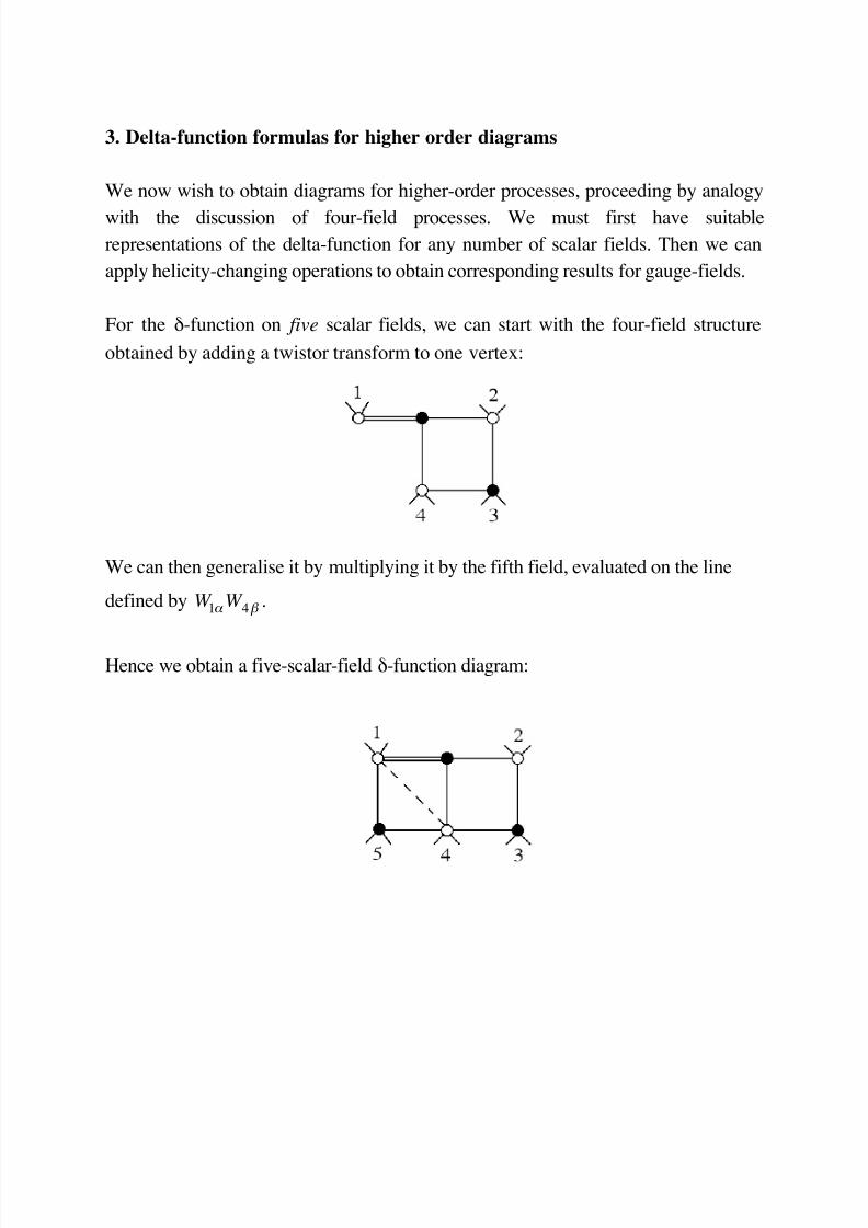
For the δ-function on five scalar fields, we can start with the four-field structure

obtained by adding a twistor transform to one vertex:

We can then generalise it by multiplying it by the fifth field, evaluated on the line

defined by W 1α W 4β .

Hence we obtain a five-scalar-field δ-function diagram:



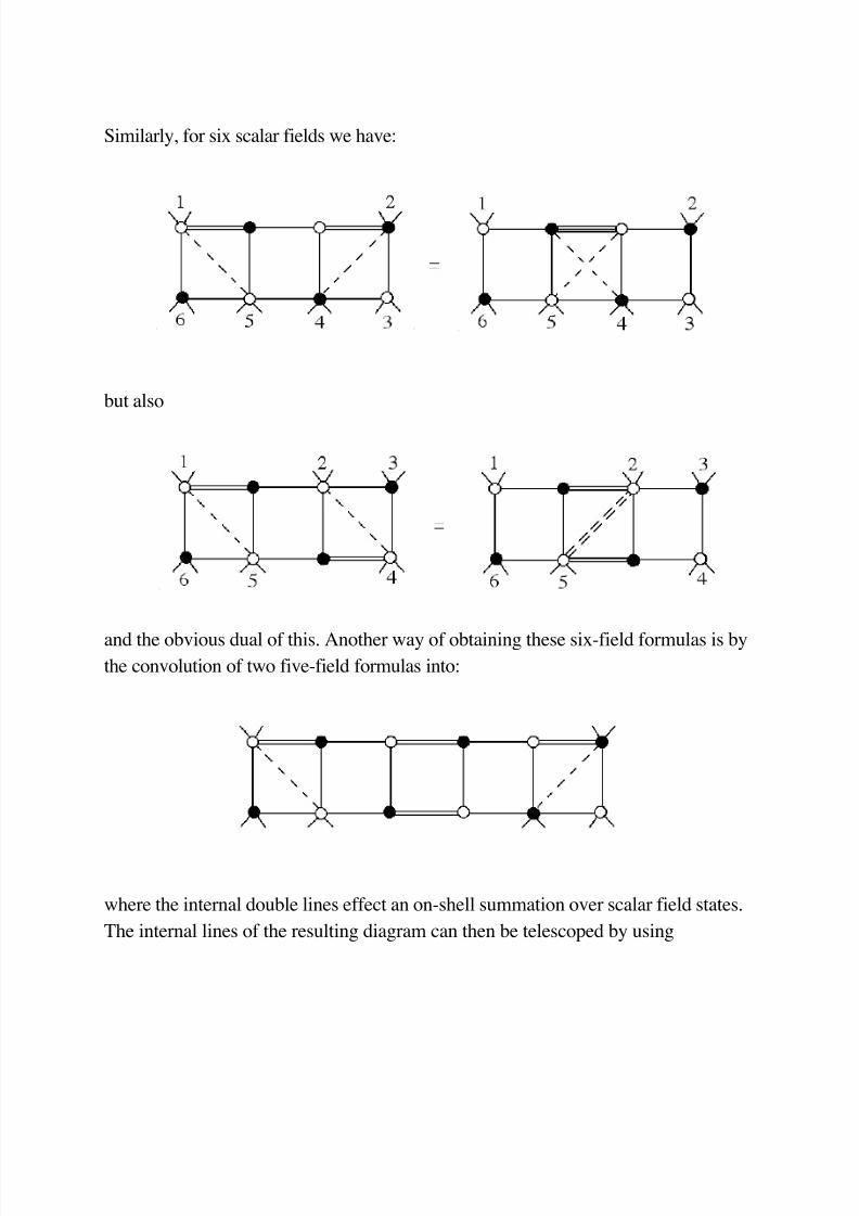
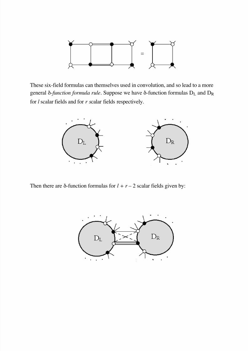
Similarly, for six scalar fields we have:

but also

and the obvious dual of this. Another way of obtaining these six-field formulas is bythe convolution of two five-field formulas into:

where the internal double lines effect an on-shell summation over scalar field states.

The internal lines of the resulting diagram can then be telescoped by using



These six-field formulas can themselves used in convolution, and so lead to a more

general δ-function formula rule. Suppose we have δ-function formulas DL and DR

for l scalar fields and for r scalar fields respectively.

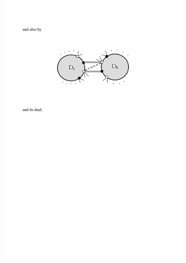
Then there are δ-function formulas for l + r – 2 scalar fields given by:



and also by

and its dual.



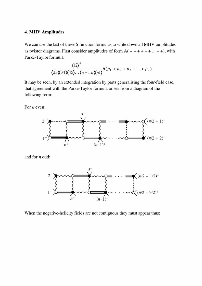
4. MHV Amplitudes

We can use the last of these δ-function formulas to write down all MHV amplitudes

as twistor diagrams. First consider amplitudes of form A( – – + + + + ... + +), with

Parke-Taylor formula

123

23 34 45 K n −1,n n1δ ( p1 + p2 + p3 +K + pn )

It may be seen, by an extended integration by parts generalising the four-field case,

that agreement with the Parke-Taylor formula arises from a diagram of the

following form:

For n even:

and for n odd:

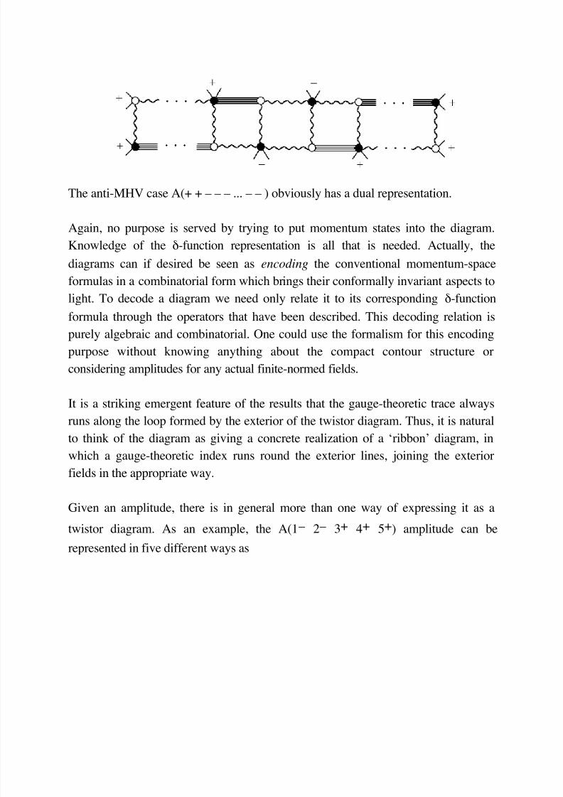
When the negative-helicity fields are not contiguous they must appear thus:



The anti-MHV case A(+ + – – – ... – – ) obviously has a dual representation.

Again, no purpose is served by trying to put momentum states into the diagram.

Knowledge of the δ-function representation is all that is needed. Actually, the

diagrams can if desired be seen as encoding the conventional momentum-space

formulas in a combinatorial form which brings their conformally invariant aspects to

light. To decode a diagram we need only relate it to its corresponding δ-function

formula through the operators that have been described. This decoding relation is

purely algebraic and combinatorial. One could use the formalism for this encoding

purpose without knowing anything about the compact contour structure or

considering amplitudes for any actual finite-normed fields.

It is a striking emergent feature of the results that the gauge-theoretic trace always

runs along the loop formed by the exterior of the twistor diagram. Thus, it is natural

to think of the diagram as giving a concrete realization of a ‘ribbon’ diagram, in

which a gauge-theoretic index runs round the exterior lines, joining the exterior

fields in the appropriate way.

Given an amplitude, there is in general more than one way of expressing it as a

twistor diagram. As an example, the A(1 – 2 – 3+ 4+ 5+) amplitude can be

represented in five different ways as



These diagrams should be interpreted as representing some deeper twistor-

geometric entity. In particular, there are identities and linear dependences between

diagrams which differ only in their boundary lines. This is only to be expected as

such identities and linear relations simply reflect linear relations betweencorresponding contours: i.e. the pure geometry of twistor space.

We shall be able to characterise this multiplicity of representation in another way, by

applying the result which will be obtained in the next section.



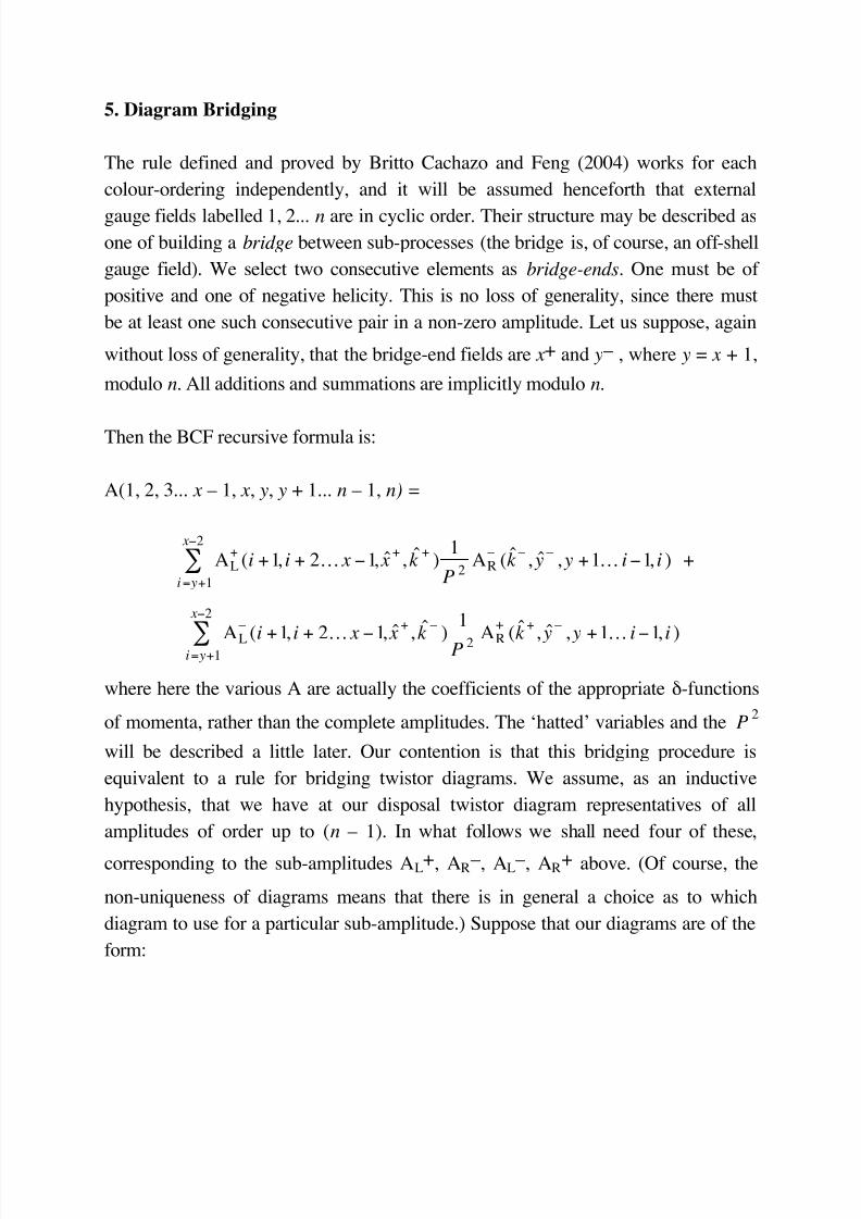
5. Diagram Bridging

The rule defined and proved by Britto Cachazo and Feng (2004) works for each

colour-ordering independently, and it will be assumed henceforth that external

gauge fields labelled 1, 2... n are in cyclic order. Their structure may be described as

one of building a bridge between sub-processes (the bridge is, of course, an off-shell

gauge field). We select two consecutive elements as bridge-ends. One must be of

positive and one of negative helicity. This is no loss of generality, since there must

be at least one such consecutive pair in a non-zero amplitude. Let us suppose, again

without loss of generality, that the bridge-end fields are x+ and y – , where y = x + 1,

modulo n. All additions and summations are implicitly modulo n.

Then the BCF recursive formula is:

A(1, 2, 3... x – 1, x, y, y + 1... n – 1, n) =

AL+

(i +1, i + 2K x −1, ˆ x+

, k +

)1

P 2AR

–(k

–, ˆ y

–, y +1K i−1, i )

i= y+1

x−2

∑ +

AL

–

(i+

1, i+

2K x −1, ˆ x

+

,ˆk

–

)

1

P 2 AR

+

(ˆk

+

, ˆ y

–

, y+

1K i−1, i )i= y+1

x−2

∑

where here the various A are actually the coefficients of the appropriate δ-functions

of momenta, rather than the complete amplitudes. The ‘hatted’ variables and the P2

will be described a little later. Our contention is that this bridging procedure is

equivalent to a rule for bridging twistor diagrams. We assume, as an inductive

hypothesis, that we have at our disposal twistor diagram representatives of all

amplitudes of order up to (n – 1). In what follows we shall need four of these,

corresponding to the sub-amplitudes AL+, AR

–, AL –, AR

+ above. (Of course, the

non-uniqueness of diagrams means that there is in general a choice as to which

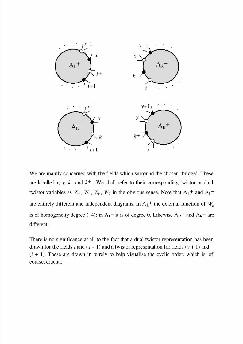
diagram to use for a particular sub-amplitude.) Suppose that our diagrams are of the

form:



We are mainly concerned with the fields which surround the chosen ‘bridge’. These

are labelled x, y, k – and k + . We shall refer to their corresponding twistor or dual

twistor variables as Z x , W y , Z k , W k in the obvious sense. Note that AL+ and AL

–

are entirely different and independent diagrams. In AL+ the external function of W k

is of homogeneity degree (–4); in AL – it is of degree 0. Likewise AR

+ and AR – are

different.

There is no significance at all to the fact that a dual twistor representation has beendrawn for the fields i and ( x – 1) and a twistor representation for fields ( y + 1) and

(i + 1). These are drawn in purely to help visualise the cyclic order, which is, of

course, crucial.



We have made a choice about the Z x , W y , Z k , W k variables which form the

‘bridge’, but this choice has no deep significance because twistor transforms can

always be used to change the representation.

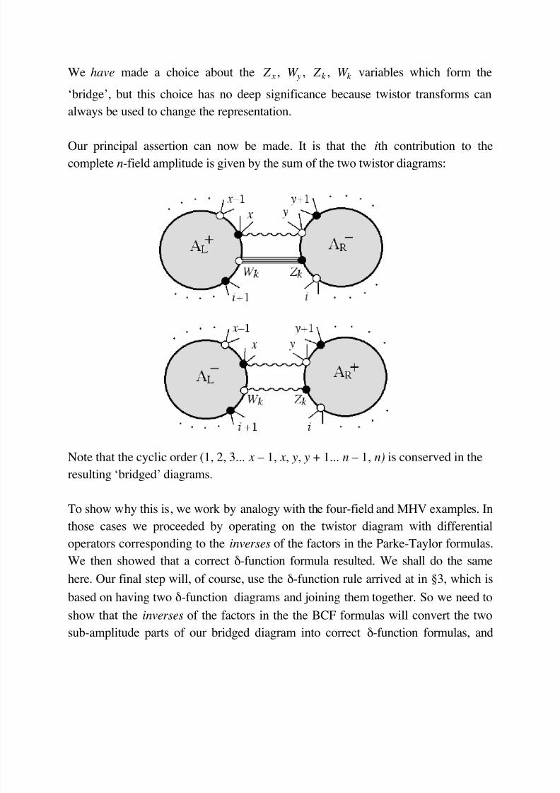
Our principal assertion can now be made. It is that the ith contribution to the

complete n-field amplitude is given by the sum of the two twistor diagrams:

Note that the cyclic order (1, 2, 3... x – 1, x, y, y + 1... n – 1, n) is conserved in the

resulting ‘bridged’ diagrams.

To show why this is, we work by analogy with the four-field and MHV examples. In

those cases we proceeded by operating on the twistor diagram with differential

operators corresponding to the inverses of the factors in the Parke-Taylor formulas.

We then showed that a correct δ-function formula resulted. We shall do the same

here. Our final step will, of course, use the δ-function rule arrived at in §3, which is

based on having two δ-function diagrams and joining them together. So we need to

show that the inverses of the factors in the the BCF formulas will convert the two

sub-amplitude parts of our bridged diagram into correct δ-function formulas, and



also produce the correct form of bridge between the two.

The key idea is that the ‘hatted’ spinors as defined by Britto Cachazo and Feng are

exactly defined so as to correspond to this twistor diagram operation. To make the

connection, recall that all the spinor objects used in momentum-space formulas

appear in the twistor diagram as combinations of

I αβ

W rβ , I αβ Z sβ

, I αβ ∂ / ∂W rβ , I αβ

∂ / ∂ Z sβ

We shall use the shorter notation W r A

, Z s ′ A , ∂W r ′ A , ∂ Z s A

for these.

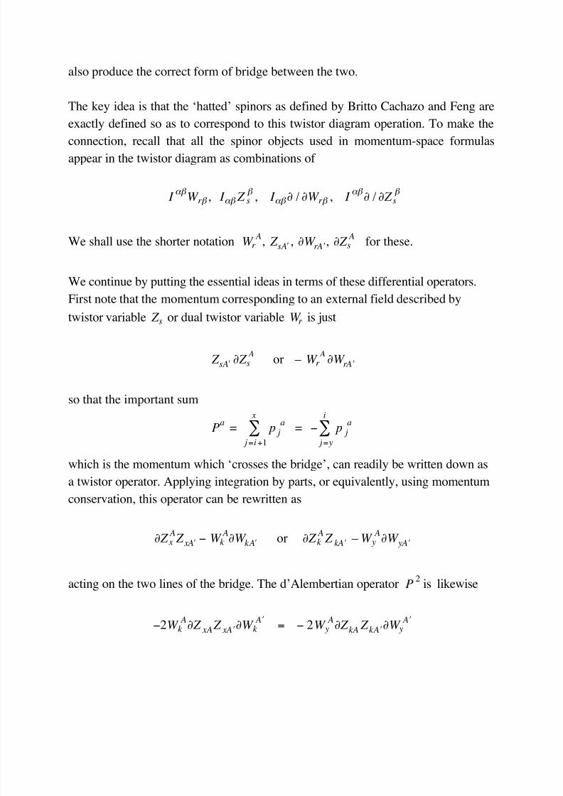
We continue by putting the essential ideas in terms of these differential operators.

First note that the momentum corresponding to an external field described by

twistor variable Z s or dual twistor variable W r is just

Z s ′ A ∂ Z s A

or – W r A

∂W r ′ A

so that the important sum

Pa

= p j a

j =i+1

x∑ = − p j

a

j = y

i∑

which is the momentum which ‘crosses the bridge’, can readily be written down as

a twistor operator. Applying integration by parts, or equivalently, using momentum

conservation, this operator can be rewritten as

∂ Z x A Z x ′ A − W k

A∂W k ′ A or ∂ Z k

A Z k ′ A – W y

A∂W y ′ A

acting on the two lines of the bridge. The d’Alembertian operator P2

is likewise

−2W k A∂ Z xA Z x ′ A ∂W k

′ A= − 2W y

A∂ Z kA Z k ′ A ∂W y

′ A



Now consider the effect of ∂ Z x A

. If it were left unmodified in the bridged diagrams,

it would act on the boundary line joining it to W y , and this would prevent the sub-

amplitude twistor diagrams being correctly reduced to their corresponding

δ-function formulas. So it must be modified in such a way that it becomes ‘blind’ tothe bridge. The modification is:

∂ ˆ Z x A

= ∂ Z x A

− 12

P 2W y A

W y B P B ′ A Z x

′ A= ∂ Z x

A−W y

A Z k

′ A∂W

y ′ A

Z k ′ B Z

x ′ B

and similarly

∂W y ′ A = ∂W y ′ A − 12

P2 Z

x ′ A

W y A P A ′ B Z x

′ B= ∂W y ′ A − Z x ′ A

W k A∂ Z

xA

W k BW

yB

These operators, acting on the two lines of the bridge, vanish. They will therefore

behave within the bridged diagrams exactly as ∂ Z x A

, ∂W y ′ A did in the separate sub-

amplitudes. Note that the definition using P determines these operators in terms of

the actual external fields of the bridged diagram.

Likewise, the k operators must be such as to act on the sub-amplitude parts of the

bridged diagrams just as the k operators did within the separated components.

Moreover, ∂W k ′ A must be defined so that it is equivalent to ˆ Z k ′ A and ∂ ˆ Z kA likewise

equivalent to W kA . Before defining them, note that:

∂ Z k A

= W k A Z

x ′ A∂W k

′ A

Z x ′ B Z k ′

B

and ∂W k ′ A = Z x ′ A

W y A∂ Z

kA

W y BW kB

We also have: W kA∂W k ′ A = Z x ′ A ∂ Z kA

Following Britto Cachazo and Feng, we can satisfy all these demands by:



∂W k ′ A = ˆ Z k ′ A =P A ′ A W y

A

W y B

P B ′ B Z x′ B

= Z

k ′ A

Z k ′ B

Z x′ B

∂ ˆ Z kA

= W kA

= P A ′

A Z

x

′ A= W

kA Z

x ′

A∂W

k

′ A

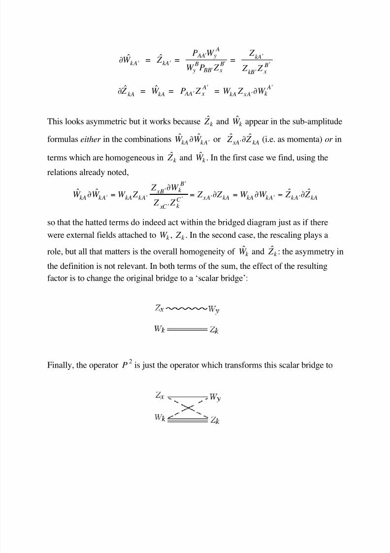
This looks asymmetric but it works because ˆ Z k and W k appear in the sub-amplitude

formulas either in the combinations W kA∂W k ′ A or ˆ Z x ′ A ∂ ˆ Z kA (i.e. as momenta) or in

terms which are homogeneous in ˆ Z k and W k . In the first case we find, using the

relations already noted,

W kA∂W k ′ A = W kA Z k ′ A

Z x ′

B

∂W k

′ B

Z x ′ C

Z k ′ C

= Z x ′ A ∂ Z kA = W kA∂W k ′ A = ˆ Z k ′ A ∂ ˆ Z kA

so that the hatted terms do indeed act within the bridged diagram just as if there

were external fields attached to W k , Z k . In the second case, the rescaling plays a

role, but all that matters is the overall homogeneity of W k and ˆ Z k : the asymmetry in

the definition is not relevant. In both terms of the sum, the effect of the resulting

factor is to change the original bridge to a ‘scalar bridge’:

Finally, the operator P2

is just the operator which transforms this scalar bridge to



Now that the twistor equivalents of the BCF hatted spinor definitions are known,

and their properties noted, we can apply the strategy as described above to show

the correspondence between the BCF formula and the bridged twistor diagrams.

Thinking of the formula as defining operators applied to the δ-function, we apply the

corresponding inverse operators to the bridged twistor diagrams. These operators

are such that they act on the two components just as if the bridge were not there,

except that the bridge is transformed into just the correct form for the application of

the δ-function rule. We deduce that the whole expression, operating on the bridged

diagram, will produce a δ-function formula for n fields. But this is exactly what we

require to establish the result claimed.

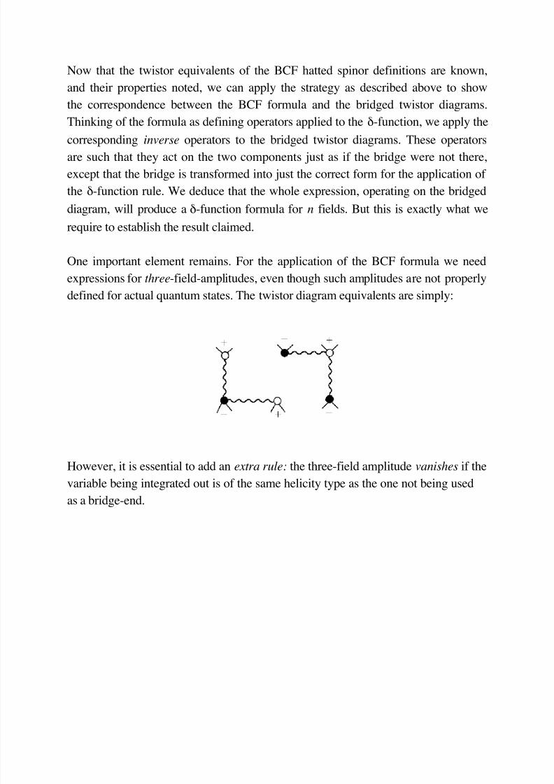
One important element remains. For the application of the BCF formula we need

expressions for three-field-amplitudes, even though such amplitudes are not properly

defined for actual quantum states. The twistor diagram equivalents are simply:

However, it is essential to add an extra rule: the three-field amplitude vanishes if the

variable being integrated out is of the same helicity type as the one not being used

as a bridge-end.



6. Examples of diagram bridging to find non-MHV amplitudes

It is now straightforward to write down the terms arising in the application of the

BCF formula. It is useful to verify the production of 4 and 5-field MHV processes

from 3-vertex terms. This is instructive because we learn from this that the

ambiguity of expression in these amplitudes is exactly accounted for by the different

possible choices of where to build the bridges. However, we will go straight to the

non-MHV processes.

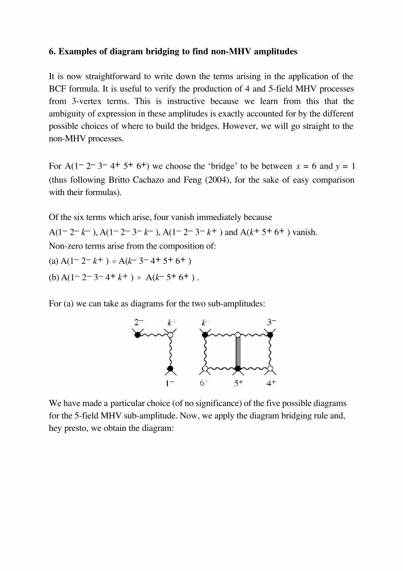
For A(1 – 2 – 3 – 4+ 5+ 6+) we choose the ‘bridge’ to be between x = 6 and y = 1

(thus following Britto Cachazo and Feng (2004), for the sake of easy comparison

with their formulas).

Of the six terms which arise, four vanish immediately because

A(1 – 2 – k – ), A(1 – 2 – 3 – k – ), A(1 – 2 – 3 – k + ) and A(k + 5+ 6+ ) vanish.

Non-zero terms arise from the composition of:

(a) A(1 – 2 – k + ) o A(k – 3 – 4+ 5+ 6+ )

(b) A(1 – 2 – 3 – 4+ k + ) o A(k – 5+ 6+ ) .

For (a) we can take as diagrams for the two sub-amplitudes:

We have made a particular choice (of no significance) of the five possible diagrams

for the 5-field MHV sub-amplitude. Now, we apply the diagram bridging rule and,

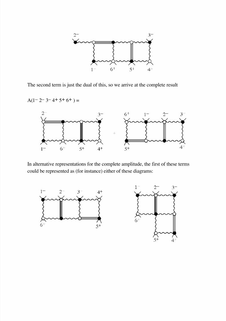
hey presto, we obtain the diagram:



The second term is just the dual of this, so we arrive at the complete result

A(1 – 2 – 3 – 4+ 5+ 6+ ) =

In alternative representations for the complete amplitude, the first of these terms

could be represented as (for instance) either of these diagrams:



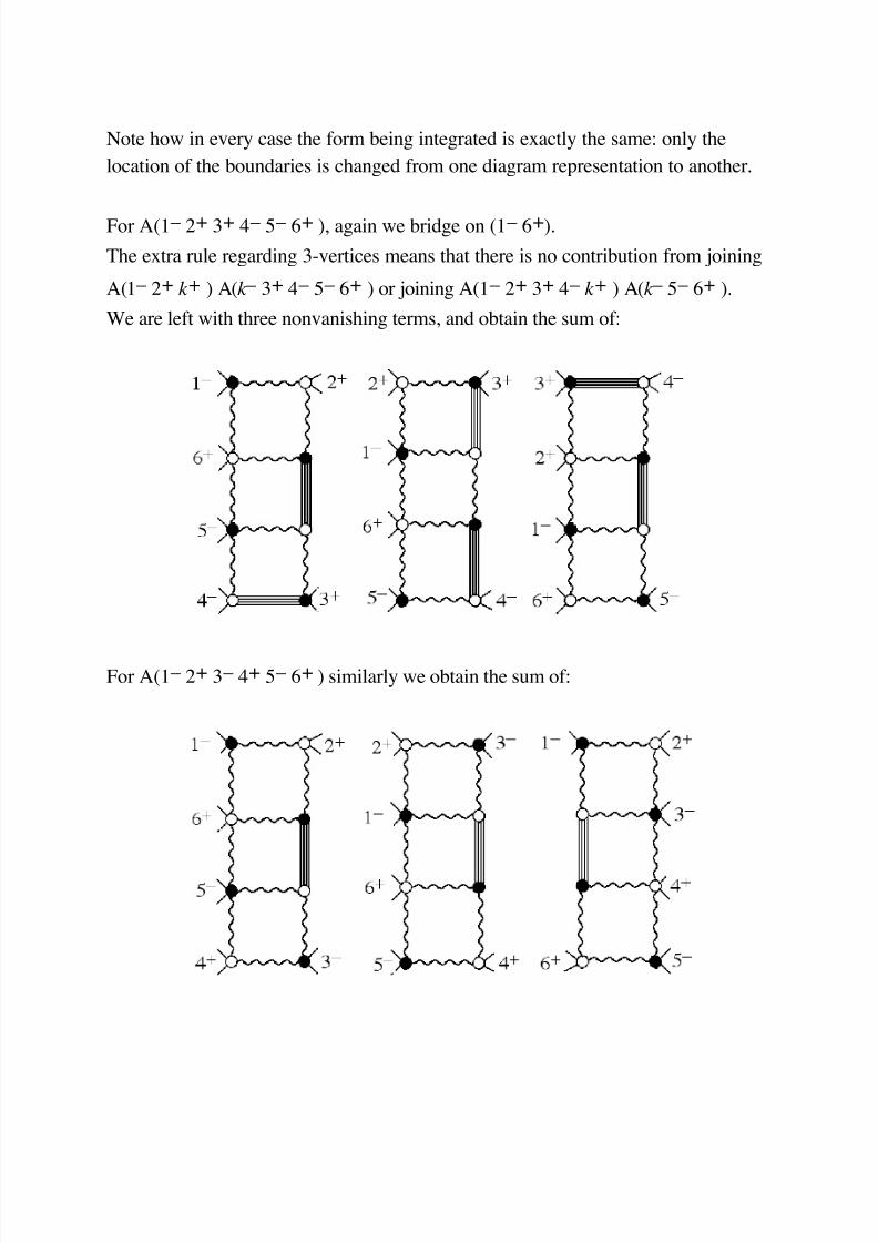
Note how in every case the form being integrated is exactly the same: only the

location of the boundaries is changed from one diagram representation to another.

For A(1 – 2+ 3+ 4 – 5 – 6+ ), again we bridge on (1 – 6+).

The extra rule regarding 3-vertices means that there is no contribution from joining

A(1 – 2+ k + ) A(k – 3+ 4 – 5 – 6+ ) or joining A(1 – 2+ 3+ 4 – k + ) A(k – 5 – 6+ ).

We are left with three nonvanishing terms, and obtain the sum of:

For A(1 – 2+ 3 – 4+ 5 – 6+ ) similarly we obtain the sum of:



The usefulness of this representation has been verified by studying twistor diagrams

for the seven-field and eight-field tree amplitudes computed by Britto Cachazo and

Feng (2004), also by Roiban, Spradlin and Volovich (2004), Bern, Del Duca, Dixon,

and Kosower (2004). In some cases, the diagram representation makes it easier to

see the identity of various terms that arise. However, the important and difficult

linear dependences between various formulas, as noted by these authors, cannot be

be read off directly from this new diagram representation. We can only say that the

geometry of the diagrams opens the door to a completely new description of such

relationships, based on the pure homology theory (more accurately, the relative

homology) of the integration space. We add a few remarks on this development in

the next section.



7. Twistor Quilts

The striking geometric relationship of the diagram to the gauge-theoretic trace

obviously suggests a relationship with open strings. (This connection was noticed

long ago (Hodges 1990, 1998) but in woeful ignorance of the astonishing

generalisation already effected by Parke, Taylor (1986) and others, its potential was

not properly appreciated!) We are naturally led to the suggestion that the non-

unique representation of amplitudes by diagrams can be understood in terms of

these different but equivalent diagrams being merely different ways of dividing up

an underlying string-like object. These divisions are not so much like ribbons as like

quilts. It seems very likely that different ‘quilts’ for a given amplitude can be

expressed entirely in terms of different choices of bridge-ends in applications of the

bridging process.

A striking fact is that it is that it is not actually necessary to specify which lines

represent the quadruple poles, and which are the boundaries. If an external field is of

homogeneity (–4), it ‘forces’ the lines meeting its vertex to be boundary lines, and

these in turn force the others. It will be found that all the diagrams have sufficient

external (–4) functions to determine the identity of all the internal lines. This feature

of the diagrams seems to be intimately related to the rule about vanishing 3-vertices.

It would also seem to be related to the very nature of tree diagrams. Just asFeynman diagrams for tree amplitudes carry momenta which are fully determined

by the external fields, so tree twistor diagrams carry helicities which are likewise

uniquely specified. ( Ipso facto, we expect this property to fail for loop diagrams.)

In these tree diagrams one could actually replace each quadruple pole by a

boundary line, together with the numerical factor (24 k –4), and the result of the

integration would be the same. In this way, everything in the diagram becomes pure

geometry. This again strongly suggests that identities and linear relationships

between amplitudes are equivalent to purely geometrical relationships between

homology classes.

To specify a twistor diagram, then, it suffices to list the ordering of vertices and the

input of external fields. We can illustrate this by drawing streamlined ‘quilt’



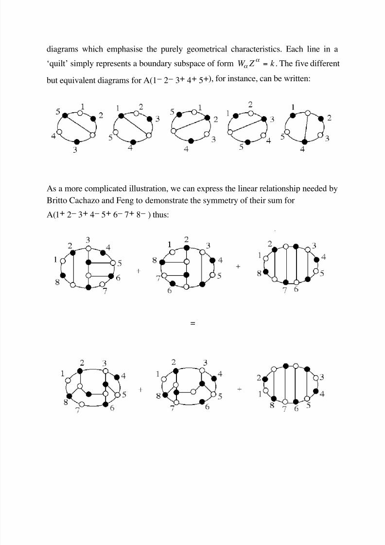
diagrams which emphasise the purely geometrical characteristics. Each line in a

‘quilt’ simply represents a boundary subspace of form W α Z α = k . The five different

but equivalent diagrams for A(1 – 2 – 3+ 4+ 5+), for instance, can be written:

As a more complicated illustration, we can express the linear relationship needed byBritto Cachazo and Feng to demonstrate the symmetry of their sum for

A(1+ 2 – 3+ 4 – 5+ 6 – 7+ 8 – ) thus:

=



These six ‘quilts’ correspond to the expressions described by Britto Cachazo and

Feng as W , g5rW , X , g

2T , g

7T , g

7V respectively. Indeed they encode all the

information in those expressions. It seems possible that this will lead to useful

combinatorial methods for establishing identities.

Obviously, the diagrams are helpful in seeing discrete symmetries, but it is perhaps

even more important that they bring to light the essential elements of conformal

symmetry which have not hitherto been emphasised. The apparently weird rational

functions of momenta which appear in the long formulas for these amplitudes, can

surely now be better understood as the outcome of applying conformally invariant

operators — a tightly defined range of combinatorial and algebraic ingredients.

But perhaps the most vivid feature of the twistor diagrams is that they tell a

physically significant story about the process. The story lies in the ‘cut’ structure,

where we immediately see the collinear and multiparticle singularities corresponding

to physically possible sub-processes. It should be possible also to derive a simple rule

for what happens when an external gauge-field is ‘dropped’, since rough inspection

shows that if external fields of homogeneity degree 0 are simply chopped off, a new

contour emerges which yields the correct amplitude for the corresponding process

with one less field. These reduction phenomena are in themselves strong constraints

on the forms that the diagrams can take, and suggest that useful theorems can be

gained by combining them with analytic S-matrix insights.



8. Extension to loop diagrams

Can these results be extended to loop diagrams? There are encouraging signs.

Although the focus of this note has been on gauge fields, twistor diagrams are

equally applicable to other zero-rest-mass field theories. It is straightforward to write

down tree diagrams for massless scalar field theory, and there are obvious

candidates (as yet unverified) for structures corresponding to one-loop scalar

diagrams. If this can be verified, it should be possible to use a twistor diagram

version of the ‘box-function’ as a template for the gauge-theoretic one-loop

diagrams in analogy with the use of the simple δ-function scalar diagrams for tree

diagrams, and so obtain analogous one-loop gauge-theoretic expressions. It is

noteworthy that the amplitude formulas obtained by ‘cutting’ loop diagrams do fit

with the twistor-diagram representation, and this again suggests there is something

important to be found at the loop level. It is also noteworthy that the twistor

diagrams have so strong a connection with ‘cut’ structure.

However, considerable caution is required. We do not know which theory we

expect to find at this level: N=0 or N=4 or something else again? It is not clear

whether the ultra-violet divergence structure can be handled correctly within the

formalism, although for infra-red divergences, the structure already discussed at tree

level seems very promising. And there will in general be information in Feynman

loop diagrams that does not appear in their cut structure: we have no evidence that

any such information will be correctly supplied by a twistor-diagram formalism.

An interesting possibility is that for loop-like diagram lines, where helicities are not

determined by external fields, the inhomogeneity will liberate the twistor line-

propagators from interpretation in terms of helicity eigenstates and give something

quite new.



9. Further implications

If we study the the internal vertices in these twistor diagrams, we note an internal

twistor vertex for every departure from MHV. Dually, there is a dual-twistor

internal vertex for every departure from anti-MHV. There seems to be a definite

connection with the pictures called ‘twistor diagrams’ in the theory of Witten

(2003), showing how external fields can be considered as confined to lines, or more

generally several intersecting lines, in twistor space, with the number of lines

determined by the departure from MHV.

Edward Witten’s theory has already led to much greater understanding of the

twistor diagram structure for tree amplitudes, and how this should be related to one-loop diagrams. There is doubtless much more to be learnt.

The correspondence with Witten’s theory is, however, indirect. If our line-

propagators were all simple poles then they could be thought of as restricting all the

variables involved to certain lines in twistor space. But instead, they are the third

derivatives of, or the inverse derivatives of, such poles. Another, more radical,

difference lies in the inhomogeneity employed in our formalism. Thus the structures

remarked on in this note cannot simply be deductions from Witten’s theory.

Finally, the diagram recursion principle gives a clear indication of an autonomous

generating principle. The recursion relation can be put in terms of rules for the

composition of 3-field amplitudes. It should be likewise possible to derive rules for

generating twistor diagrams from formal 3-vertices, in a Lagrangian-like form. The

‘ribbon’ aspect of the diagrams also suggests a connection with the beautiful

geometric ideas of string theory which have inspired so many advances. In

conclusion, I express indebtedness to the tireless ingenuity of the quantum fieldtheorists who have revealed such astonishing structure in this formidable problem.



Acknowledgements

I am grateful for the opportunity to discuss some of these ideas with Roger Penrose,

Philip Candelas, Valentin Khoze, Lionel Mason, and David Skinner. I am also in

debt to all those who organised and spoke at the conference on twistors and strings

at Oxford University in January 2005, and so stimulated these new observations.

References:

Z. Bern, V. Del Duca, L. J. Dixon and D. A. Kosower, All non-maximally helicity-violating one-

loop seven-gluon amplitudes in N=4 super-Yang-Mills theory, hep-th/0410224 (2004)

R. Britto, F. Cachazo and B. Feng, Recursion relations for tree amplitudes of gluons,hep-th/0412308 (2004)

A. P. Hodges, A twistor approach to the regularisation of divergences. Proc. Roy. Soc. Lond. A

397, 341 (1985)

A. P. Hodges, Twistor diagrams, in T. N. Bailey and R. J. Baston (eds.), Twistors in Mathematics

and Physics, Cambridge University Press (1990)

A. P. Hodges, The twistor diagram programme, in The Geometric Universe: Science, Geometry

and the Work of Roger Penrose, eds. S. A Huggett, L. J. Mason, K. P. Tod, S. T. Tsou, N. M. J.

Woodhouse, Oxford University Press (1998)

S. Parke and T. Taylor, An amplitude for N gluon scattering, Phys. Rev. Lett. 56, 2459 (1986)

R. Penrose and M. A. H. MacCallum, Twistor theory: an approach to the quantisation of fields and

space-time, Physics Reports 4, 241 (1972)

R. Penrose, Twistor theory, its aims and achievements, in Quantum Gravity, eds. C. J. Isham, R.

Penrose and D. W. Sciama, Oxford University Press (1975)

R. Roiban, M. Spradlin and A. Volovich, Dissolving N=4 amplitudes into QCD tree amplitudes,

hep-th/0412265 (2004)

E. Witten, Perturbative gauge theory as a string theory in twistor space, hep-th/0312171 (2003)

Further supporting material will appear on http://www.twistordiagrams.org.uk

andrew hodges- twistor diagram recursion for all gauge-theoretic tree amplitudes

Documents