Angelic Hierarchical Planning: Optimal and OnlineAlgorithms

Bhaskara MarthiStuart J. RussellJason Wolfe

Electrical Engineering and Computer SciencesUniversity of California at Berkeley

Technical Report No. UCB/EECS-2008-150

http://www.eecs.berkeley.edu/Pubs/TechRpts/2008/EECS-2008-150.html

December 6, 2008

Copyright 2008, by the author(s).All rights reserved.

Permission to make digital or hard copies of all or part of this work forpersonal or classroom use is granted without fee provided that copies arenot made or distributed for profit or commercial advantage and that copiesbear this notice and the full citation on the first page. To copy otherwise, torepublish, to post on servers or to redistribute to lists, requires prior specificpermission.

Acknowledgement

Bhaskara Marthi thanks Leslie Kaelbling and Tomas Lozano-Perez foruseful discussions. This researchwas also supported by DARPA IPTO, contracts FA8750-05-2-0249 andFA8750-07-D-0185 (subcontract 03-000219).

Angelic Hierarchical Planning: Optimal and Online Algorithms

Bhaskara Marthi BHASKARA@CSAIL.MIT.EDU

MIT/Willow Garage Inc.

Stuart Russell RUSSELL@CS.BERKELEY.EDU

Computer Science Division, University of California, Berkeley, CA 94720

Jason Wolfe∗ JAWOLFE@CS.BERKELEY.EDU

Computer Science Division, University of California, Berkeley, CA 94720

Abstract

High-level actions (HLAs) are essential tools for coping with the large search spaces and long decisionhorizons encountered in real-world decision making. In a recent paper, we proposed an “angelic” semanticsfor HLAs that supports proofs that a high-level plan will (or will not) achieve a goal, without first reducing theplan to primitive action sequences. This paper extends the angelic semantics with cost information to supportproofs that a high-level plan is (or is not) optimal. We describe the Angelic Hierarchical A* algorithm, whichgenerates provably optimal plans, and show its advantages over alternative algorithms. We also present theAngelic Hierarchical Learning Real-Time A* algorithm for situated agents, one of the first algorithms to dohierarchical lookahead in an online setting. Since high-level plans are much shorter, this algorithm can lookmuch farther ahead than previous algorithms (and thus choose much better actions) for a given amount ofcomputational effort. This is an extended version of a paper by the same name appearing in ICAPS ’08.

1. IntroductionHumans somehow manage to choose quite intelligently the twenty trillion primitive motor commands thatconstitute a life, despite the large state space. It has long been thought that hierarchical structure in behavioris essential in managing this complexity. Structure exists at many levels, ranging from small (hundred-step?)motor programs for typing characters and saying phonemes up to large (billion-step?) actions such as writingan ICAPS paper, getting a good faculty position, and so on. The key to reducing complexity is that one canchoose (correctly) to write an ICAPS paper without first considering all the character sequences one mighttype.

Hierarchical planning attempts to capture this source of power. It has a rich history of contributions (towhich we cannot do justice here) going back to the seminal work of Tate (1977). The basic idea is to supplya planner with a set of high-level actions (HLAs) in addition to the primitive actions. Each HLA admits oneor more refinements into sequences of (possibly high-level) actions that implement it. Hierarchical plannerssuch as SHOP2 (Nau et al., 2003) usually consider only plans that are refinements of some top-level HLAs forachieving the goal, and derive power from constraints placed on the search space by the refinement hierarchy.

One might hope for more; consider, for example, the downward refinement property: every plan thatclaims to achieve some condition does in fact have a primitive refinement that achieves it. This property wouldenable the derivation of provably correct abstract plans without refining all the way to primitive actions,providing potentially exponential speedups. This requires, however, that HLAs have clear precondition–effect semantics, which have until recently been unavailable (McDermott, 2000). In a recent paper (Marthiet al., 2007) — henceforth (MRW ’07) — we defined an “angelic semantics” for HLAs, specifying for eachHLA the set of states reachable by some refinement into a primitive action sequence. The angelic approachcaptures the fact that the agent will choose a refinement and can thereby choose which element of an HLA’sreachable set is actually reached. This semantics guarantees the downward refinement property and yields

∗. The authors appear in alphabetical order.

1

a sound and complete hierarchical planning algorithm that derives significant speedups from its ability togenerate and commit to provably correct abstract plans.

Our previous paper ignored action costs and hence our planning algorithm used no heuristic information,a mainstay of modern planners. The first objective of this paper is to rectify this omission. The angelicapproach suggests the obvious extension: the exact cost of executing a high-level action to get from state s tostate s′ is the least cost among all primitive refinements that reach s′. In practice, however, representing theexact cost of an HLA from each state s to each reachable state s′ is infeasible, and we develop concise lowerand upper bound representations. From this starting point, we derive the first algorithm capable of generatingprovably optimal abstract plans. Conceptually, this algorithm is an elaboration of A*, applied in hierarchicalplan space and modified to handle the special properties of refinement operators and use both upper and lowerbounds. We also provide a satisficing algorithm that sacrifices optimality for computational efficiency andmay be more useful in practice. Preliminary experimental results show that these algorithms outperform both“flat” and our previous hierarchical approaches.

The paper also examines HLAs in the online setting, wherein an agent performs a limited lookahead priorto selecting each action. The value of lookahead has been amply demonstrated in domains such as chess.We believe that hierarchical lookahead with HLAs can be far more effective because it brings back to thepresent value information from far into the future. Put simply, it’s better to evaluate the possible outcomesof writing an ICAPS paper than the possible outcomes of choosing “A” as its first character. We derive anangelic hierarchical generalization of Korf’s LRTA* (1990), which shares LRTA*’s guarantees of eventualgoal achievement on each trial and eventually optimal behavior after repeated trials. Experiments show thatthis algorithm substantially outperforms its nonhierarchical ancestor.

2. Background2.1 Planning Problems

Deterministic, fully observable planning problems can be described in a representation-independent mannerby a tuple (S, s0, t,L, T, g), where S is a set of states, s0 is the initial state, t is the goal state,1 L is a setof primitive actions, and T : S × L → S and g : S × L → R+ are transition and cost functions such thatdoing action a in state s leads to state T (s, a) with cost g(s, a).2 These functions are overloaded to operate onsequences of actions in the obvious way: if a = (a1, . . . , am), then T (s,a) = T (. . . T (s, a1) . . . , am) andg(s,a) is the total cost of this sequence. The objective is to find a solution a ∈ L∗ for which T (s0,a) = t.

Definition 1. A solution a∗ is optimal iff it reaches the goal with minimal cost:

a∗ = arg mina∈L∗:T (s0,a)=t g(s0,a).

We assume the state and action spaces are finite. To ensure that optimal solutions exist, we also assumethat there is at least one finite-cost solution, and every cycle in the state space has positive cost. In thispaper, we will represent S as the set of truth assignments to some set of ground propositions, and T using theSTRIPS language (Fikes and Nilsson, 1971).

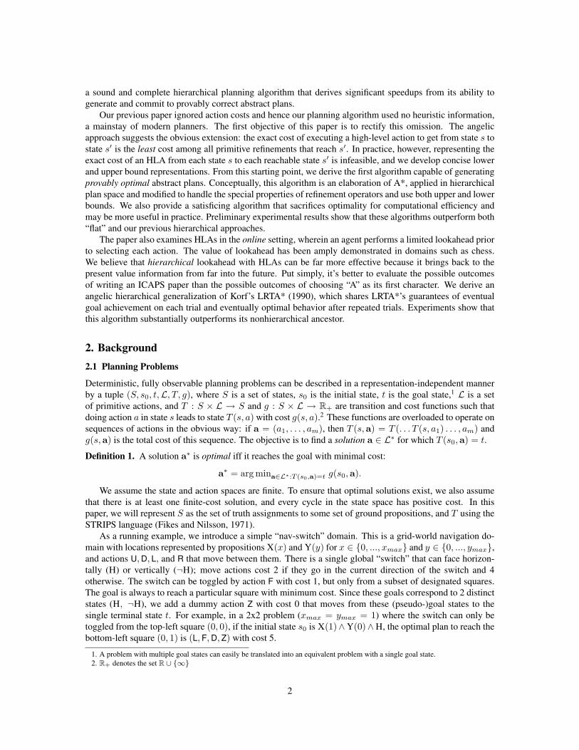
As a running example, we introduce a simple “nav-switch” domain. This is a grid-world navigation do-main with locations represented by propositions X(x) and Y(y) for x ∈ {0, ..., xmax} and y ∈ {0, ..., ymax},and actions U, D, L, and R that move between them. There is a single global “switch” that can face horizon-tally (H) or vertically (¬H); move actions cost 2 if they go in the current direction of the switch and 4otherwise. The switch can be toggled by action F with cost 1, but only from a subset of designated squares.The goal is always to reach a particular square with minimum cost. Since these goals correspond to 2 distinctstates (H, ¬H), we add a dummy action Z with cost 0 that moves from these (pseudo-)goal states to thesingle terminal state t. For example, in a 2x2 problem (xmax = ymax = 1) where the switch can only betoggled from the top-left square (0, 0), if the initial state s0 is X(1)∧Y(0)∧H, the optimal plan to reach thebottom-left square (0, 1) is (L, F, D, Z) with cost 5.

1. A problem with multiple goal states can easily be translated into an equivalent problem with a single goal state.2. R+ denotes the set R ∪ {∞}

2

2.2 High-Level Actions

In addition to a planning problem, our algorithms will be given a set A of high-level actions, along with aset I(a) of allowed immediate refinements for each HLA a ∈ A. Each immediate refinement consists of afinite sequence a ∈ A∗, where we define A = A∪L as the set of all actions. Each HLA and refinement mayhave an associated precondition, which specifies conditions under which its use is appropriate.3 To make ahigh-level sequence more concrete we may refine it, by replacing one of its HLAs by one of its immediaterefinements, and we call one plan a refinement of another if it is reachable by any sequence of such steps.A primitive refinement consists only of primitive actions, and we define I∗(a, s) as the set of all primitiverefinements of a that obey all HLA and refinement preconditions when applied from state s. We assume noplan is a refinement of itself. Finally, we assume a special top-level action Act∈A, and restrict our attentionto plans in I∗(Act, s0).

Definition 2. (Parr and Russell, 1998) A plan ah∗ is hierarchically optimal iff

ah∗ = arg mina∈I∗(Act,s0):T (s0,a)=tg(s0,a).

Remark. Because the hierarchy may constrain the set of allowed sequences, g(s0,ah∗) ≥ g(s0,a∗).

When equality holds from all possible initial states, the hierarchy is called optimality-preserving.The hierarchy for our running example has three HLAs: A = {Nav, Go, Act}. Nav(x, y) navigates

directly to location (x, y); it can refine to the empty sequence iff the agent is already at (x, y), and otherwiseto any primitive move action followed by a recursive Nav(x, y). Go(x, y) is like Nav, except that it mayflip the switch on the way; it either refines to (Nav(x, y)), or to (Nav(x′, y′), F, Go(x, y)) where (x′, y′) canaccess the switch. Finally, Act is the top-level action, which refines to (Go(xg, yg), Z), where (xg, yg) is thegoal location. This hierarchy is optimality-preserving for any instance of the nav-switch domain.

3. Cost-Based Descriptions of HLAsAs mentioned in the introduction, our angelic semantics (MRW ’07) describes the outcome of a high-levelplan by its reachable set of states (by some refinement). However, these reachable sets say nothing aboutcosts incurred along the way. This section describes a novel extension of the angelic approach that includescost information. This will allow us to find good plans quickly by focusing on better-seeming plans first, andpruning provably suboptimal high-level plans without refining them further.

We begin with the notion of an exact description Ea of an HLA a, which specifies, for each pair of states(s, s′), the minimum cost of any primitive refinement of a that leads from s to s′ (this generalizes the originaldefinition from (MRW ’07)).

Definition 3. The exact description of HLA a is a function Ea(s)(s′) = minb∈I∗(a,s):T (s,b)=s′ g(s,b).

Remark. Note that the set of primitive refinements may be infinite. The minimum must still be attained,however, due to the finiteness and positive-cycle assumptions.

Remark. Definition 3 implies that if s′ is not reachable from s by any refinement of a, Ea(s)(s′) = ∞.

Definition 4. A valuation is a function v : S → R+. The initial valuation v0 has v0(s0) = 0 and v0(s) = ∞for all s 6= s0.

We can think of descriptions as functions from states to valuations that specify a reachable set plus a finitecost for each reachable state (see Figure 1(b)). Then, descriptions can be extended to functions from valua-tions to valuations, by defining Ea(v)(s′) = mins∈S v(s) + Ea(s)(s′). Finally, these extended descriptionscan be composed to produce descriptions for high-level sequences.

3. We treat these preconditions as advisory, so for our purposes a planning algorithm is complete even if it takes them into account,and sound even if it ignores them.

3

Definition 5. Given a sequence a = (a1, . . . , aN ), the exact transition function of a is a function mappingvaluations to valuations: Ea = EaN

◦ . . . ◦ Ea1 .

Theorem 1. For any integer N , final state sN , and action sequence a ∈ AN , the minimum over all statesequences (s1, ..., sN−1) of total cost

∑Ni=1 Eai(si−1)(si) equals Ea(v0)(sN ). Moreover, for any such mini-

mizing state sequence, concatenating the primitive refinements of each HLA ai that achieve the minimum costEai(si−1)(si) for each step yields a primitive refinement of a that reaches sN from s0 with minimal cost.

Proof. The proof is by induction. When N = 1, the theorem follows trivially from Definitions 3 and 4.When N > 1,

min(s1,...,sN−1)

N∑i=1

Eai(si−1)(si) = min(s1,...,sN−1)

(EaN

(sN−1)(sN ) +N−1∑i=1

Eai(si−1)(si)

)

= minsN−1

(EaN

(sN−1)(sN ) + min(s1,..,sN−2)

N−1∑i=1

Eai(si−1)(si)

)= min

sN−1

(EaN

(sN−1)(sN ) + EaN−1 ◦ . . . ◦ Ea1(v0)(sN−1))

= EaN◦ . . . ◦ Ea1(v0)(sN )

By this theorem, an efficient, compact representation for Ea would (under mild conditions) lead to anefficient optimal planning algorithm. Unfortunately, since deciding even simple plan existence is PSPACE-hard (Bylander, 1994), we cannot hope for this in general. We will therefore consider principled compactapproximations to Ea that still allow for precise inferences about the effects and costs of high-level plans.

3.1 Optimistic and Pessimistic Bounds on Descriptions

Definition 6. A valuation v1 (weakly) dominates another valuation v2, written v1 � v2, iff(∀s ∈ S) v1(s) ≤ v2(s).

Definition 7. An optimistic description Oa of HLA a satisfies (∀s) Oa(s) � Ea(s).

For example, our optimistic description of Go (see Figure 1(a/c)) specifies that the cost for getting tothe target location (possibly flipping the switch on the way) is at least twice its Manhattan distance from thecurrent location; moreover, all other states are unreachable by Go.

Definition 8. A pessimistic description Pa of HLA a satisfies (∀s) Ea(s) � Pa(s).

For example, our pessimistic description of Go specifies that the cost to reach the destination is at mostfour times its Manhattan distance from the current location.

Remark. For primitive actions a ∈ L, Oa(s)(s′) = Pa(s)(s′) = g(s, a) iff s′ = T (s, a),∞ otherwise.

Optimistic and pessimistic descriptions generalize our previous complete and sound descriptions (MRW’07). In this paper, we will assume that the descriptions are given along with the hierarchy. However, we notethat it is theoretically possible to derive them automatically from the structure of the hierarchy.

As with exact descriptions, we can extend optimistic and pessimistic descriptions and then composethem to produce bounds on the outcomes of high-level sequences, which we call optimistic and pessimisticvaluations (see Figure 1(c/d)).

Theorem 2. Given any sequence a ∈ AN and state s, the cost c = minb∈I∗(a,s0)|T (s0,b)=s g(s0,b) of thebest primitive refinement of a that reaches s from s0 satisfies OaN

◦ . . . ◦ Oa1(v0)(s) ≤ c ≤ PaN◦ . . . ◦

Pa1(v0)(s).

4

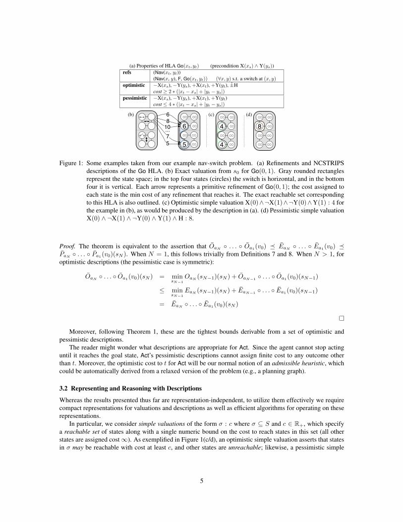
(a) Properties of HLA Go(xt, yt) (precondition X(xs) ∧ Y(ys))refs (Nav(xt, yt))

(Nav(x, y), F, Go(xt, yt)) (∀x, y) s.t. a switch at (x, y)optimistic −X(xs), −Y(ys), +X(xt), +Y(yt), ±H

cost ≥ 2 ∗ (|xt − xs|+ |yt − ys|)pessimistic −X(xs), −Y(ys), +X(xt), +Y(yt)

cost ≤ 4 ∗ (|xt − xs|+ |yt − ys|)

∞ ∞

6 ∞

∞ ∞

5 ∞

6

8

7

5

(b) (c) (d)

10...

∞ ∞

4 ∞

∞ ∞

4 ∞

∞ ∞

8 ∞

∞ ∞

∞ ∞

Figure 1: Some examples taken from our example nav-switch problem. (a) Refinements and NCSTRIPSdescriptions of the Go HLA. (b) Exact valuation from s0 for Go(0, 1). Gray rounded rectanglesrepresent the state space; in the top four states (circles) the switch is horizontal, and in the bottomfour it is vertical. Each arrow represents a primitive refinement of Go(0, 1); the cost assigned toeach state is the min cost of any refinement that reaches it. The exact reachable set correspondingto this HLA is also outlined. (c) Optimistic simple valuation X(0)∧¬X(1)∧¬Y(0)∧Y(1) : 4 forthe example in (b), as would be produced by the description in (a). (d) Pessimistic simple valuationX(0) ∧ ¬X(1) ∧ ¬Y(0) ∧ Y(1) ∧ H : 8.

Proof. The theorem is equivalent to the assertion that OaN◦ . . . ◦ Oa1(v0) � EaN

◦ . . . ◦ Ea1(v0) �PaN

◦ . . . ◦ Pa1(v0)(sN ). When N = 1, this follows trivially from Definitions 7 and 8. When N > 1, foroptimistic descriptions (the pessimistic case is symmetric):

OaN◦ . . . ◦ Oa1(v0)(sN ) = min

sN−1OaN

(sN−1)(sN ) + OaN−1 ◦ . . . ◦ Oa1(v0)(sN−1)

≤ minsN−1

EaN(sN−1)(sN ) + EaN−1 ◦ . . . ◦ Ea1(v0)(sN−1)

= EaN◦ . . . ◦ Ea1(v0)(sN )

Moreover, following Theorem 1, these are the tightest bounds derivable from a set of optimistic andpessimistic descriptions.

The reader might wonder what descriptions are appropriate for Act. Since the agent cannot stop actinguntil it reaches the goal state, Act’s pessimistic descriptions cannot assign finite cost to any outcome otherthan t. Moreover, the optimistic cost to t for Act will be our normal notion of an admissible heuristic, whichcould be automatically derived from a relaxed version of the problem (e.g., a planning graph).

3.2 Representing and Reasoning with Descriptions

Whereas the results presented thus far are representation-independent, to utilize them effectively we requirecompact representations for valuations and descriptions as well as efficient algorithms for operating on theserepresentations.

In particular, we consider simple valuations of the form σ : c where σ ⊆ S and c ∈ R+, which specifya reachable set of states along with a single numeric bound on the cost to reach states in this set (all otherstates are assigned cost∞). As exemplified in Figure 1(c/d), an optimistic simple valuation asserts that statesin σ may be reachable with cost at least c, and other states are unreachable; likewise, a pessimistic simple

5

valuation asserts that each state in σ is reachable with cost at most c, and other states may be reachable aswell.4

Simple valuations are convenient, since we can reuse our previous machinery (MRW ’07) for reasoningwith reachable sets represented as DNF (disjunctive normal form) logical formulae and HLA descriptionsspecified in a language called NCSTRIPS (Nondeterministic Conditional STRIPS). NCSTRIPS is an exten-sion of ordinary STRIPS that can express a set of possible effects with mutually exclusive conditions. Eacheffect consists of four lists of propositions: add (+), delete (−), possibly-add (+), and possibly-delete (−).Added propositions are always made true in the resulting state, whereas possibly-added propositions may ormay not be made true; in a pessimistic description, the agent can force either outcome, whereas in an opti-mistic one the outcome may not be controllable. By extending NCSTRIPS with cost bounds (which can becomputed by arbitrary code), we produce descriptions suitable for the approach taken here. Figure 1(a) showspossible descriptions for Go in this extended language (as is typically the case, these descriptions could bemade more accurate at the expense of conciseness by conditioning on features of the initial state).

With these representational choices, we require an algorithm for progressing a simple valuation repre-sented as a DNF reachable set plus numeric cost bound through an extended NCSTRIPS description. Ifwe perform this progression exactly, the output may not be a simple valuation (since different states in thereachable set may produce different cost bounds). Thus, we will instead consider an approximate progressionalgorithm that projects results back into the space of simple valuations. Applying this algorithm repeatedlywill allow us to compute optimistic and pessimistic simple valuations for entire high-level sequences.

The algorithm is a simple extension of that given in (MRW ’07), which progresses each (conjunctiveclause, conditional effect) pair separately and then disjoins the results. This progression proceeds by (1)conjoining effect conditions onto the clause (and skipping this clause if a contradiction is created), (2) makingall added (resp. deleted) literals true (resp. false), and finally (3) removing literals from the clause if false(resp. true) and possibly-added (resp. possibly-deleted). With our extended NCSTRIPS descriptions, each(clause, effect) pair also produces a cost bound. When progressing optimistic (resp. pessimistic) valuations,we simply take the min (resp. max) of all these bounds plus the initial bound to get the cost bound for thefinal valuation.5

Our above definitions need some minor modifications to allow for such approximate progression algo-rithms. For simplicity, we will absorb any additional approximation into our notation for the descriptionsthemselves:

Definition 9. An approximate progression algorithm corresponds to, for each extended optimistic and pes-simistic description Oa and Pa, (further) approximated descriptions Oa and Pa. Call the algorithm correctif, for all actions a and valuations v, Oa(v) � Oa(v) and Pa(v) � Pa(v).

Intuitively, a progression algorithm is correct as long as the errors it introduces only further weaken thedescriptions.

Theorem 3. Theorem 2 still holds if we use any correct approximate progression algorithm, replacing eachOa and Pa with its further approximated counterpart Oa and Pa.

The proof is similar to that of Theorem 2.

4. Offline Search AlgorithmsThis section describes algorithms for the offline planning setting, in which the objective is to quickly find alow-cost sequence of actions leading all the way from s0 to t.

4. More interesting tractable classes of valuations are possible; for instance, rather than using a single numeric bound, we could allowlinear combinations of indicator functions on state variables.

5. A more accurate algorithm for pessimistic progression sorts the clauses by increasing pessimistic cost, computes the minimal prefixof this list whose disjunction covers all of the remaining clauses, and then restricts the max over cost bounds to clauses in this prefix.We did not implement this version, since it requires many potentially expensive subsumption checks.

6

{s10h}:0

{s10h}:0

{s00h}:2

{s00h}:2

[2, 2]

[1, 1] [2, 4]

{s01h,s01v}:5

{s01v} :7

+0

+2

+4

+2

(a)

(b)

2

4

4

1

2

{t}:10

{t}:10

{t}:5

{t}:7

[0, 0] {t}:6

{t}:6

[0, 0]

[0, 0]

{s00h}:2

{s00h}:2[2, 2]

[0, 0]

[2, 2]

[6, 6]...

{s00v}:3

{s00v}:3

[4, 4]

{s10h}:4

{s10h}:4

{s01h}:6

{s01h}:6{s01h}:6

{s01h}:6

{s01h}:10

{s01h}:10

s10h :0

s00h :2

s11h :4

s01h :6

s00v :3

s10h :4

L

D

R

Nav01

Nav00

Go01F

Z

L

D

D

R

F

Z

Z

Nav01

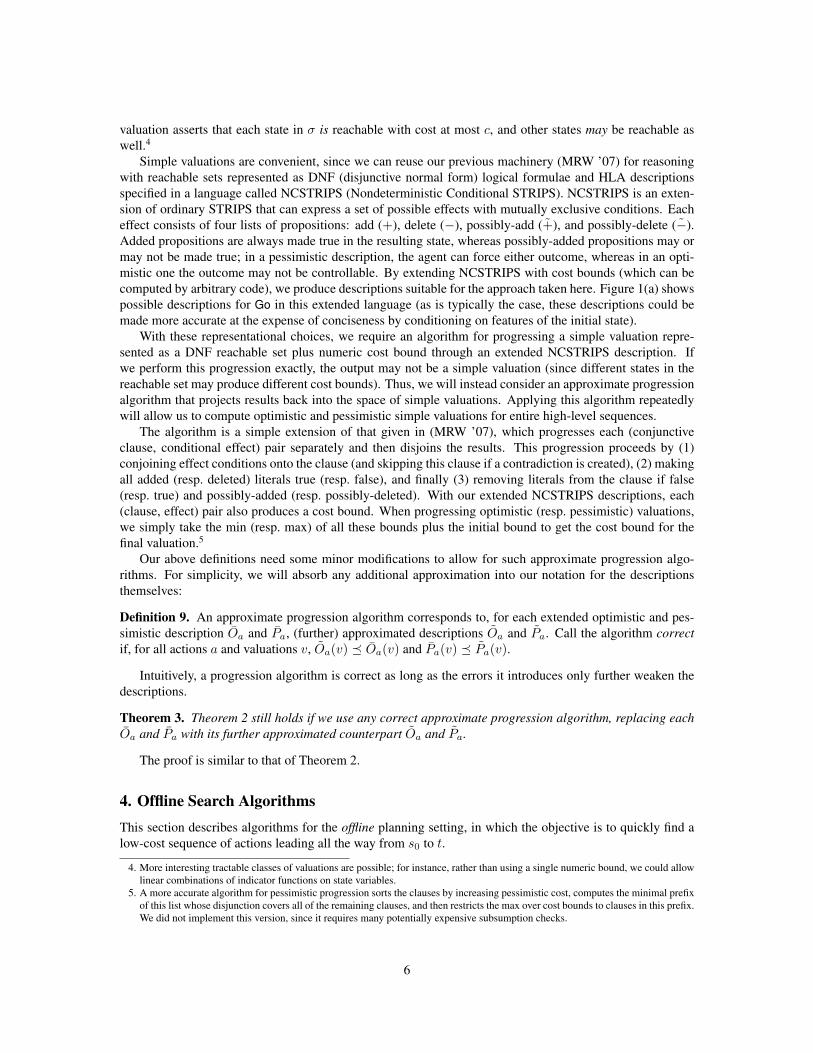
Figure 2: (a) A standard lookahead tree for our example. Nodes are labeled with states (written sxy(h/v))and costs-so-far, edges are labeled with actions and associated costs, and leaves have a heuristicestimate of the remaining distance-to-goal. (b) An abstract lookahead tree (ALT) for our example.Nodes are labeled with optimistic and pessimistic simple valuations and edges are labeled with(possibly high-level) actions and associated optimistic and pessimistic costs.

Because we have models for our HLAs, our planning algorithms will resemble existing algorithms thatsearch over primitive action sequences. Such algorithms typically operate by building a lookahead tree(see Figure 2(a)). The initial tree consists of a single node labeled with the initial state and cost 0, andcomputations consist of leaf node expansions: for each primitive action a, we add an outgoing edge labeledwith that action and its cost g(s, a), whose child is labeled with the state s′ = T (s, a) and total cost to s′. Wealso include at leaf nodes a heuristic estimate h(s′) of the remaining cost to the goal. Paths from the root to aleaf are potential plans; for each such plan a, we estimate the total cost of its best continuation by f(s0,a) =g(s0,a) + h(T (s0,a)), the sum of its cost and heuristic value. If the heuristic h never overestimates, wecall it admissible, and this f -cost will also never overestimate. If h also obeys the triangle inequality h(s) ≤g(s, a)+h(T (s, a)), we call it consistent, and expanding a node will always produce extensions with greateror equal f -cost. These properties are required for A* and its graph version (respectively) to efficiently findoptimal plans.

In hierarchical planning we will consider algorithms that build abstract lookahead trees (ALTs). Inan ALT, edges are labeled with (possibly high-level) actions and nodes are labeled with optimistic andpessimistic valuations for corresponding partial plans. For example, in the ALT in Figure 2(b), by doing(Nav(0, 0), F, Go(0, 1)), state s01v is definitely reachable with cost in [5, 7], s01h may be reachable withcost at least 5, and no other states are possibly reachable. Since our planning algorithms will try to findlow-cost solutions, we will be most concerned with finding optimistic (and pessimistic) bounds on the costof the best primitive refinement of each high-level plan that reaches t. These bounds can be extracted di-rectly from the final ALT node of each plan; for instance, the optimistic and pessimistic costs to t of plan(Nav(0, 0), F, Go(0, 1), Z) are [5, 7].

In a generalization of the ordinary notion of consistency, we will sometimes desire consistent HLA de-scriptions, under which we never lose information by refining.6 As in the flat case, when descriptions areconsistent, the optimistic cost to t (i.e., f -cost) of a plan will never decrease with further refinement. Simi-larly, its best pessimistic cost will never increase.

6. Specifically, a set of optimistic descriptions (plus approximate progression algorithm, if applicable) is consistent iff, when werefine any high-level plan, its optimistic valuation dominates the optimistic valuations of its refinements. A set of pessimisticdescriptions (plus progression algorithm) is consistent iff the state-wise minimum of a set of refinements’ pessimistic valuationsalways dominates the pessimistic valuation of the parent plan.

7

We first describe our ALT data structures and how they address some of the issues that arise in ourhierarchical planning framework in novel ways. We then present our optimal planning algorithm, AHA*, andbriefly describe an alternative “satisficing” algorithm, AHSS.

4.1 Abstract Lookahead Trees

Our ALT data structures support our search algorithms by efficiently managing a set of candidate high-levelplans and associated valuations. The issues involved differ from the primitive setting because nodes storevaluations rather than single states and exact costs, and because (unlike node expansion) plan refinement is“top-down” and may not correspond to simple extensions of existing plans.

Algorithm 1 shows pseudocode for some basic ALT operations. Our search algorithms work by firstcreating an ALT containing some initial set of plans using MAKEINITIALALT, and then repeatedly refiningcandidate plans using REFINEPLANEDGE, which only considers refinements whose preconditions are metby at least one state in the corresponding optimistic reachable set. Both operations internally call ADDPLAN,which adds a plan to the ALT by starting at the existing node corresponding to the longest prefix shared withany existing plan, and creating nodes for the remaining plan suffix by progressing its valuations through thecorresponding action descriptions. In the process, partial plans that are provably dominated and plans thatcannot possibly reach the goal are recognized and skipped over.

Theorem 4. If a node n with optimistic valuation O(n) is created while adding plan a, and another noden′ exists with pessimistic valuation P (n′) s.t. P (n′) � O(n) and the remaining plan suffix of a is a legalhierarchical continuation from n′, then a is safely prunable.

Proof. We must show that if any primitive refinement of a is hierarchically optimal, then there exists aprimitive refinement of a plan passing through n′ that is hierarchically optimal as well (and thus we don’tlose hierarchical optimality by pruning a). Suppose that b ∈ I∗(s0,a) is hierarchically optimal with costc. Decompose a into a1, the set of actions leading up to node n, and a2, the remainder of the actions ina. Decompose b similarly, so that b1 ∈ I∗(s0,a1), and b2 ∈ I∗(s,a2), where s = T (s0,b1) and byhierarchical optimality of b, T (s,b2) = t. Let c1 = g(s0,b1) and c2 = g(s,b2) so that c = c1 + c2. Now,by the definition of optimistic descriptions, we must have O(n)(s) ≤ c1. Let c be the sequence of actionsleading up to n′. Because P (n′) � O(n), we must have P (n′)(s) ≤ c1. Thus, by definition of pessimisticdescriptions, there exists d ∈ I∗(s0, c) such that T (s0,d) = s and g(s0,d) ≤ c1. Finally, since a2 isan allowed continuation from n′, concatenating d and b2 yields a primitive plan that reaches t, is a validhierarchical primitive refinement of a plan passing through n′, and has total cost ≤ c. Thus, either b was nothierarchically optimal in the first place, or this new refinement of a plan passing through n′ is hierarchicallyoptimal as well.

Remark. The continuation condition is needed since the hierarchy might allow better continuations fromnode n than n′.

For example, the plan (L, R, Nav(0, 1), Z) in Figure 2(b) is prunable since its optimistic valuation is dom-inated by the pessimistic valuation above it, and the empty continuation is allowed from that node. Sincedetecting all pruned nodes can be very expensive, our implementation only considers pruning for nodes withsingleton reachable sets.

One might wonder why REFINEPLANEDGE refines a single plan at a given HLA edge, rather than simul-taneously refining all plans that pass through it. The reason is that after each refinement of the HLA, it wouldhave to continue progression for each such plan’s suffix. This could be needlessly expensive, especially ifsome such plans are already thought to be bad.

In any case, when valuations are simple, we can use a novel improvement called upward propagation(implemented in REFINEPLANEDGE) to propagate new information about the cost of a refined HLA edgeto other plans that pass through it, without having to explicitly refine them or do any additional progression.This improvement hinges on the fact that with simple valuations, the optimistic and pessimistic costs for aplan can be broken down into optimistic and pessimistic costs for each action in that plan (see Figure 2(b)).

8

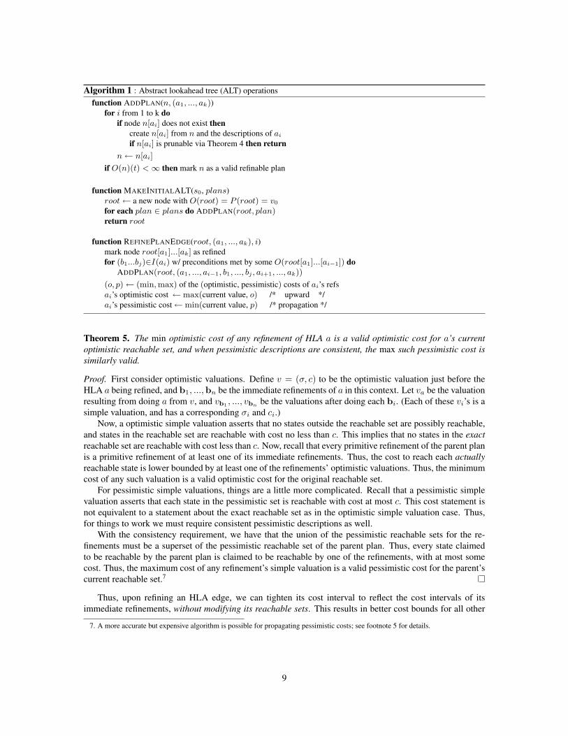
Algorithm 1 : Abstract lookahead tree (ALT) operationsfunction ADDPLAN(n, (a1, ..., ak))

for i from 1 to k doif node n[ai] does not exist then

create n[ai] from n and the descriptions of ai

if n[ai] is prunable via Theorem 4 then returnn← n[ai]

if O(n)(t) <∞ then mark n as a valid refinable plan

function MAKEINITIALALT(s0, plans)root← a new node with O(root) = P (root) = v0

for each plan ∈ plans do ADDPLAN(root, plan)return root

function REFINEPLANEDGE(root, (a1, ..., ak), i)mark node root[a1]...[ak] as refinedfor (b1...bj)∈I(ai) w/ preconditions met by some O(root[a1]...[ai−1]) do

ADDPLAN(root, (a1, ..., ai−1, b1, ..., bj , ai+1, ..., ak))

(o, p)← (min, max) of the (optimistic, pessimistic) costs of ai’s refsai’s optimistic cost ←max(current value, o) /* upward */ai’s pessimistic cost←min(current value, p) /* propagation */

Theorem 5. The min optimistic cost of any refinement of HLA a is a valid optimistic cost for a’s currentoptimistic reachable set, and when pessimistic descriptions are consistent, the max such pessimistic cost issimilarly valid.

Proof. First consider optimistic valuations. Define v = (σ, c) to be the optimistic valuation just before theHLA a being refined, and b1, ...,bn be the immediate refinements of a in this context. Let va be the valuationresulting from doing a from v, and vb1 , ..., vbn be the valuations after doing each bi. (Each of these vi’s is asimple valuation, and has a corresponding σi and ci.)

Now, a optimistic simple valuation asserts that no states outside the reachable set are possibly reachable,and states in the reachable set are reachable with cost no less than c. This implies that no states in the exactreachable set are reachable with cost less than c. Now, recall that every primitive refinement of the parent planis a primitive refinement of at least one of its immediate refinements. Thus, the cost to reach each actuallyreachable state is lower bounded by at least one of the refinements’ optimistic valuations. Thus, the minimumcost of any such valuation is a valid optimistic cost for the original reachable set.

For pessimistic simple valuations, things are a little more complicated. Recall that a pessimistic simplevaluation asserts that each state in the pessimistic set is reachable with cost at most c. This cost statement isnot equivalent to a statement about the exact reachable set as in the optimistic simple valuation case. Thus,for things to work we must require consistent pessimistic descriptions as well.

With the consistency requirement, we have that the union of the pessimistic reachable sets for the re-finements must be a superset of the pessimistic reachable set of the parent plan. Thus, every state claimedto be reachable by the parent plan is claimed to be reachable by one of the refinements, with at most somecost. Thus, the maximum cost of any refinement’s simple valuation is a valid pessimistic cost for the parent’scurrent reachable set.7

Thus, upon refining an HLA edge, we can tighten its cost interval to reflect the cost intervals of itsimmediate refinements, without modifying its reachable sets. This results in better cost bounds for all other

7. A more accurate but expensive algorithm is possible for propagating pessimistic costs; see footnote 5 for details.

9

plans that pass through this HLA edge, without needing to do any additional progression computations for(the suffixes of) such plans.8

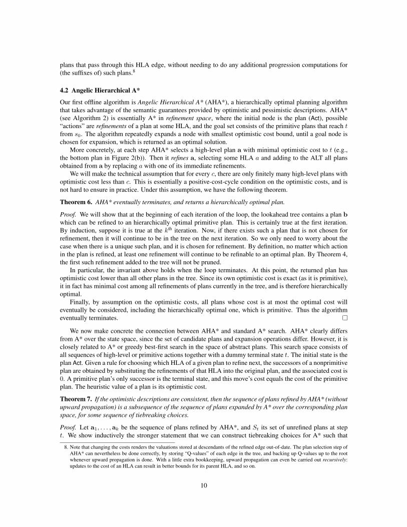
4.2 Angelic Hierarchical A*

Our first offline algorithm is Angelic Hierarchical A* (AHA*), a hierarchically optimal planning algorithmthat takes advantage of the semantic guarantees provided by optimistic and pessimistic descriptions. AHA*(see Algorithm 2) is essentially A* in refinement space, where the initial node is the plan (Act), possible“actions” are refinements of a plan at some HLA, and the goal set consists of the primitive plans that reach tfrom s0. The algorithm repeatedly expands a node with smallest optimistic cost bound, until a goal node ischosen for expansion, which is returned as an optimal solution.

More concretely, at each step AHA* selects a high-level plan a with minimal optimistic cost to t (e.g.,the bottom plan in Figure 2(b)). Then it refines a, selecting some HLA a and adding to the ALT all plansobtained from a by replacing a with one of its immediate refinements.

We will make the technical assumption that for every c, there are only finitely many high-level plans withoptimistic cost less than c. This is essentially a positive-cost-cycle condition on the optimistic costs, and isnot hard to ensure in practice. Under this assumption, we have the following theorem.

Theorem 6. AHA* eventually terminates, and returns a hierarchically optimal plan.

Proof. We will show that at the beginning of each iteration of the loop, the lookahead tree contains a plan bwhich can be refined to an hierarchically optimal primitive plan. This is certainly true at the first iteration.By induction, suppose it is true at the kth iteration. Now, if there exists such a plan that is not chosen forrefinement, then it will continue to be in the tree on the next iteration. So we only need to worry about thecase when there is a unique such plan, and it is chosen for refinement. By definition, no matter which actionin the plan is refined, at least one refinement will continue to be refinable to an optimal plan. By Theorem 4,the first such refinement added to the tree will not be pruned.

In particular, the invariant above holds when the loop terminates. At this point, the returned plan hasoptimistic cost lower than all other plans in the tree. Since its own optimistic cost is exact (as it is primitive),it in fact has minimal cost among all refinements of plans currently in the tree, and is therefore hierarchicallyoptimal.

Finally, by assumption on the optimistic costs, all plans whose cost is at most the optimal cost willeventually be considered, including the hierarchically optimal one, which is primitive. Thus the algorithmeventually terminates.

We now make concrete the connection between AHA* and standard A* search. AHA* clearly differsfrom A* over the state space, since the set of candidate plans and expansion operations differ. However, it isclosely related to A* or greedy best-first search in the space of abstract plans. This search space consists ofall sequences of high-level or primitive actions together with a dummy terminal state t. The initial state is theplan Act. Given a rule for choosing which HLA of a given plan to refine next, the successors of a nonprimitiveplan are obtained by substituting the refinements of that HLA into the original plan, and the associated cost is0. A primitive plan’s only successor is the terminal state, and this move’s cost equals the cost of the primitiveplan. The heuristic value of a plan is its optimistic cost.

Theorem 7. If the optimistic descriptions are consistent, then the sequence of plans refined by AHA* (withoutupward propagation) is a subsequence of the sequence of plans expanded by A* over the corresponding planspace, for some sequence of tiebreaking choices.

Proof. Let a1, . . . ,ak be the sequence of plans refined by AHA*, and St its set of unrefined plans at stept. We show inductively the stronger statement that we can construct tiebreaking choices for A* such that

8. Note that changing the costs renders the valuations stored at descendants of the refined edge out-of-date. The plan selection step ofAHA* can nevertheless be done correctly, by storing “Q-values” of each edge in the tree, and backing up Q-values up to the rootwhenever upward propagation is done. With a little extra bookkeeping, upward propagation can even be carried out recursively:updates to the cost of an HLA can result in better bounds for its parent HLA, and so on.

10

Algorithm 2 : Angelic Hierarchical A*function FINDOPTIMALPLAN(s0, t)

root← MAKEINITIALALT(s0, {(Act)})while ∃ an unrefined plan do

a← plan with min optimistic cost to t (tiebreak by pessimistic cost)if a is primitive then return aREFINEPLANEDGE(root,a, index of any HLA in a)

return failure

if b1, . . . ,bl denotes its sequence of expanded plans and S′t denotes its open list at step t, there exist times

1 = t1 < . . . < tk = l such that ai = btiand Si ⊆ S′

ti. The statement is clearly true for t1. Consider step i

of AHA*, which corresponds to step ti of A*. Following this step, the unrefined plans in the ALT are Si+1.At this point, the plan ai+1 is tied for the lowest cost in Si+1. S′

ti+1 contains this plan, and possibly other oneswith lower cost. However, none of those can be in Si+1. We can therefore, by making appropriate tiebreakingchoices in A*, ensure that, if ti+1 is the next time at which A* expands a plan in Si+1, bti+1 = ai+1, andfurthermore, Si+1 ⊆ S′

ti+1, completing the induction.

While AHA* might thus seem like an obvious generalization of A* to the hierarchical setting, we believethat it is an important contribution for several reasons. First, its effectiveness hinges on our ability to generatenontrivial cost bounds for high-level sequences, which did not exist previously. Second, it derives additionalpower from our ALT data structures, which provide caching, pruning, and other novel improvements specificto the hierarchical setting.

The only free parameter in AHA* is the choice of which HLA to refine in a given plan; our implementationchooses an HLA with maximal gap between its optimistic and pessimistic costs (defined below), breakingties towards higher-level actions.

Finally, we note that with consistent descriptions, as soon as AHA* finds an optimal high-level plan withequal optimistic and pessimistic costs, it will find an optimal primitive refinement very efficiently. Consis-tency ensures that after each subsequent refinement, at least one of the resulting plans will also be optimalwith equal optimistic and pessimistic costs; moreover, all but the first such plan will be pruned. Furtherrefinement of this first plan will continue until an optimal primitive refinement is found without backtracking.

4.3 Angelic Hierarchical Satisficing Search

This section presents an alternative algorithm, Angelic Hierarchical Satisficing Search (AHSS), which at-tempts to find a plan that reaches the goal with at most some pre-specified cost α. AHSS can be much moreefficient than AHA*, since it can commit to a plan without first proving its optimality.

At each step, AHSS (see Algorithm 3) begins by checking if any primitive plans succeed with cost ≤ α.If so, the best such plan is returned. Next, if any (high-level) plans succeed with pessimistic cost ≤ α, thebest such plan is committed to by discarding other potential plans. Finally, a plan with maximum priorityis refined at one of its HLAs. Priorities can be assigned arbitrarily; our implementation uses the negativeaverage of optimistic and pessimistic costs, to encourage a more depth-first search and favor plans withsmaller pessimistic cost.

Theorem 8. If there exist primitive plans consistent with the hierarchy, with cost ≤ α, AHSS eventuallyreturns one of them. Otherwise, it eventually returns failure.

Proof. The algorithm eventually terminates since there are only finitely many plans with optimistic cost≤ α.Since optimistic costs are exact for primitive plans, it will never falsely report success. Suppose there do existprimitive plans with cost ≤ α. It suffices to show that at the beginning of each iteration, the tree containsa plan one of whose primitive refinements has cost ≤ α. The invariant holds by assumption at the firstiteration. Suppose it is true at the beginning of the kth iteration. It will continue to hold after the if-statement,by definition of pessimistic costs. We only need to consider the case when there is a single such plan in the

11

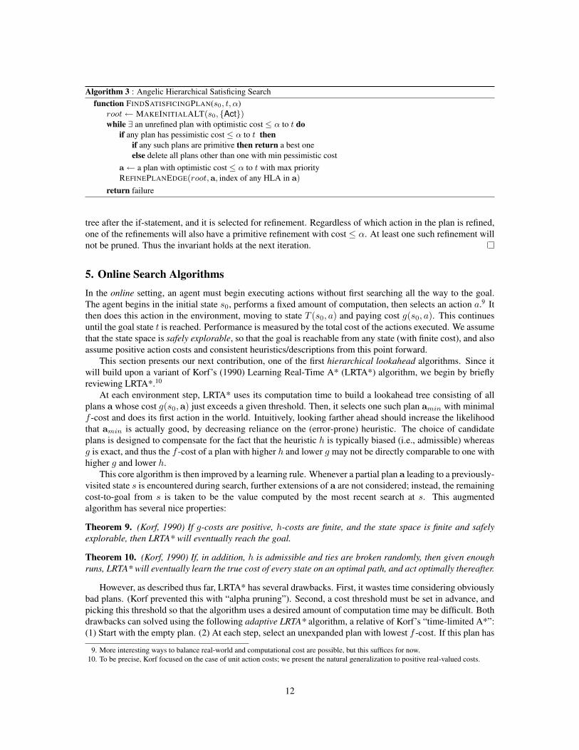
Algorithm 3 : Angelic Hierarchical Satisficing Searchfunction FINDSATISFICINGPLAN(s0, t, α)

root← MAKEINITIALALT(s0, {Act})while ∃ an unrefined plan with optimistic cost ≤ α to t do

if any plan has pessimistic cost ≤ α to t thenif any such plans are primitive then return a best oneelse delete all plans other than one with min pessimistic cost

a← a plan with optimistic cost ≤ α to t with max priorityREFINEPLANEDGE(root,a, index of any HLA in a)

return failure

tree after the if-statement, and it is selected for refinement. Regardless of which action in the plan is refined,one of the refinements will also have a primitive refinement with cost ≤ α. At least one such refinement willnot be pruned. Thus the invariant holds at the next iteration.

5. Online Search AlgorithmsIn the online setting, an agent must begin executing actions without first searching all the way to the goal.The agent begins in the initial state s0, performs a fixed amount of computation, then selects an action a.9 Itthen does this action in the environment, moving to state T (s0, a) and paying cost g(s0, a). This continuesuntil the goal state t is reached. Performance is measured by the total cost of the actions executed. We assumethat the state space is safely explorable, so that the goal is reachable from any state (with finite cost), and alsoassume positive action costs and consistent heuristics/descriptions from this point forward.

This section presents our next contribution, one of the first hierarchical lookahead algorithms. Since itwill build upon a variant of Korf’s (1990) Learning Real-Time A* (LRTA*) algorithm, we begin by brieflyreviewing LRTA*.10

At each environment step, LRTA* uses its computation time to build a lookahead tree consisting of allplans a whose cost g(s0,a) just exceeds a given threshold. Then, it selects one such plan amin with minimalf -cost and does its first action in the world. Intuitively, looking farther ahead should increase the likelihoodthat amin is actually good, by decreasing reliance on the (error-prone) heuristic. The choice of candidateplans is designed to compensate for the fact that the heuristic h is typically biased (i.e., admissible) whereasg is exact, and thus the f -cost of a plan with higher h and lower g may not be directly comparable to one withhigher g and lower h.

This core algorithm is then improved by a learning rule. Whenever a partial plan a leading to a previously-visited state s is encountered during search, further extensions of a are not considered; instead, the remainingcost-to-goal from s is taken to be the value computed by the most recent search at s. This augmentedalgorithm has several nice properties:

Theorem 9. (Korf, 1990) If g-costs are positive, h-costs are finite, and the state space is finite and safelyexplorable, then LRTA* will eventually reach the goal.

Theorem 10. (Korf, 1990) If, in addition, h is admissible and ties are broken randomly, then given enoughruns, LRTA* will eventually learn the true cost of every state on an optimal path, and act optimally thereafter.

However, as described thus far, LRTA* has several drawbacks. First, it wastes time considering obviouslybad plans. (Korf prevented this with “alpha pruning”). Second, a cost threshold must be set in advance, andpicking this threshold so that the algorithm uses a desired amount of computation time may be difficult. Bothdrawbacks can solved using the following adaptive LRTA* algorithm, a relative of Korf’s “time-limited A*”:(1) Start with the empty plan. (2) At each step, select an unexpanded plan with lowest f -cost. If this plan has

9. More interesting ways to balance real-world and computational cost are possible, but this suffices for now.10. To be precise, Korf focused on the case of unit action costs; we present the natural generalization to positive real-valued costs.

12

greater g-cost than any previously expanded plan, “lock it in” as the current return value. Expand this plan.(3) When computation time runs out, return the current “locked-in” plan.

Theorem 11. At any point during the operation of this algorithm, let a be the current locked-in plan, c2 be itscorresponding “record-setting” g-cost, and c1 be the previous record g-cost (c1 < c2). Given any thresholdin [c1, c2), LRTA* would choose a for execution (up to tiebreaking).

Proof. First, note that given any threshold c ∈ [c1, c2), LRTA* would definitely have constructed and ex-panded all of the ancestors of a. Consider any ancestor of a. By consistency and positive action costs, itmust have≤ g-cost and f -cost than a. Because a was “record-setting”, the g-cost must actually be strictly <.Now, suppose that this ancestor was not expanded. Then, its g-cost must be > c. But, c1 < c was the previousrecord-setting cost, so we have a contradiction. Thus, LRTA* would have generated but not expanded a.

Now, suppose that LRTA* with threshold c chooses some other plan over a for execution. This plan musthave cost > c to be present and unexpanded, and f -cost < that of a to be selected. But, if this was the case,this plan would have been selected for expansion by the adaptive algorithm before a, and would have beenthe previous record-setting plan. But, its cost is > c ≥ c1, the cost of the previous record-setting plan, acontradiction.

Thus, this modified algorithm can be used as an efficient, anytime version of LRTA*. Since its behaviorreduces to the original version for a particular (adaptive) choice of cost thresholds, all of the properties ofLRTA* hold for it as well.

5.1 Angelic Hierarchical Learning Real-Time A*

This section describes Angelic Hierarchical Learning Real-Time A* (AHLRTA*, see Algorithm 4), whichbears (roughly) the same relation to adaptive LRTA* as AHA* does to A*. Because a single HLA cancorrespond to many primitive actions, for a given amount of computation time we hope that AHLRTA* willhave a greater effective lookahead depth than LRTA*, and thus make better action choices. However, anumber of issues arise in the generalization to the hierarchical setting that must be addressed to make thisbasic idea work in both theory and practice.

First, while AHLRTA* searches over the space of high-level plans, when computation time runs out itmust choose a primitive action to execute. Thus, if the algorithm initializes its ALT with the single plan (Act),it will have to consider its refinements carefully to ensure that in its final ALT, at least one of the (hopefullybetter) high-level plans begins with an executable primitive. To avoid this issue (and to ensure convergenceof costs, as described below), we instead choose to initialize the ALT with the set of all plans consisting ofa primitive action followed by Act.11 With this set of plans, the choice of which HLA to refine in a plan isopen; our implementation uses the policy described above for AHA*.

Second, as we saw earlier, an analogue of f -cost can be extracted from our optimistic valuations. How-ever, there is no obvious breakdown of f into g and h components, since a high-level plan can consist ofactions at various levels, each of whose descriptions may make different types and degrees of characteristicerrors. For now, we assume that a set of higher-level HLAs (e.g., Act and Go) has been identified, let h be thesum of the optimistic costs of these actions, and let g = f − h be the cost of the primitives and remainingHLAs.

Finally, whereas the outcome of a primitive plan is a particular concrete state whose stored cost can besimply looked up in a hash table, the optimistic valuations of a high-level plan instead provide a sequenceof reachable sets of states. In general, for each such set we could look up and combine the stored costs ofits elements; instead, however, for efficiency our implementation only checks for stored costs of singletonoptimistic sets (e.g., those corresponding to a primitive prefix of a given high-level plan). If the state ina constructed singleton set has a stored cost, progression is stopped and this value is used as the cost of

11. Note that with this choice, the plans considered by the agent may not be valid hierarchical plans (i.e., refinements of Act). However,since the agent can change its mind on each world step, the actual sequence of actions executed in the world is not in generalconsistent with the hierarchy anyway.

13

Algorithm 4 : Angelic Hierarchical Learning Real-Time A*function HIERARCHICALLOOKAHEADAGENT(s0, t)

memory ← an empty hash tablewhile s0 6= t do

root← MAKEINITIALALT(s0, {(a, Act) | a ∈ L})(g, a, f)← (−1, nil, 0)while ∃ unrefined plans from root ∧ time remains do

a← a plan w/ min f -costif the g-cost of a > g then

(g,a,f)← (g-cost of a, a1, f -cost of a)

REFINEPLANEDGE(root,a, some index, memory)

do a in the worldmemory[s0]← fs0 ← T (s0, a)

the remainder of the plan. This functionality is added by modifying REFINEPLANEDGE and ADDPLANaccordingly (not shown).

Given all of these choices, we have the following:

Theorem 12. AHLRTA* reduces to adaptive LRTA*, given a “flat” hierarchy in which Act refines to anyprimitive action followed by Act (or the empty sequence).

Proof. Trivial; simply note that refining a plan in the “flat” hierarchy is the same as expanding a plan in theprimitive LRTA* setting.

(In fact, this is how we have implemented LRTA* for our experiments.) Moreover, the desirable prop-erties of LRTA* also hold for AHLRTA* in general hierarchies. This follows because AHLRTA* behavesidentically to LRTA* in neighborhoods in which every state has been visited at least once.

Theorem 13. If primitive g-costs are positive, f -costs are finite, and the state space is finite and safelyexplorable, then AHLRTA* will eventually reach the goal.

Proof. Simply note that AHLRTA* is actually equivalent to LRTA* with depth 1, where the “heuristic” iscomputed by a limited hierarchical search from each next state reachable by some primitive action.

Theorem 14. If, in addition, f -costs are admissible, ties are broken randomly, and the hierarchy is optimality-preserving, then over repeated trials AHLRTA* will eventually learn the true cost of every state on an optimalpath and act optimally thereafter.

Proof. Same as previous theorem.

If f-costs are inadmissible or the hierarchy is not optimality-preserving, the theorem still holds if s0 issampled from a distribution with support on S in each trial.

Our implementation of AHLRTA* includes two minor changes from the version described above, whichwe have found to increase its effectiveness. First, it sometimes throws away some of its allowed computationtime, so that the number of refinements taken per allowed initial primitive action is constant; this tends toimprove the interaction of the lookahead strategy with the learning rule. Second, when deciding when to“lock in” a plan it requires additionally that the plan is more refined than the previous locked in plan; thishelps counteract the implicit bias towards higher-level plans caused by aggregation of costs from primitivesand various HLAs into g-cost. Since both changes effectively only change the stopping time of the algorithm,its desirable properties are preserved.

14

6. ExperimentsThis section describes results for the above algorithms on two domains: our “nav-switch” running example,and the warehouse world (MRW ’07).12

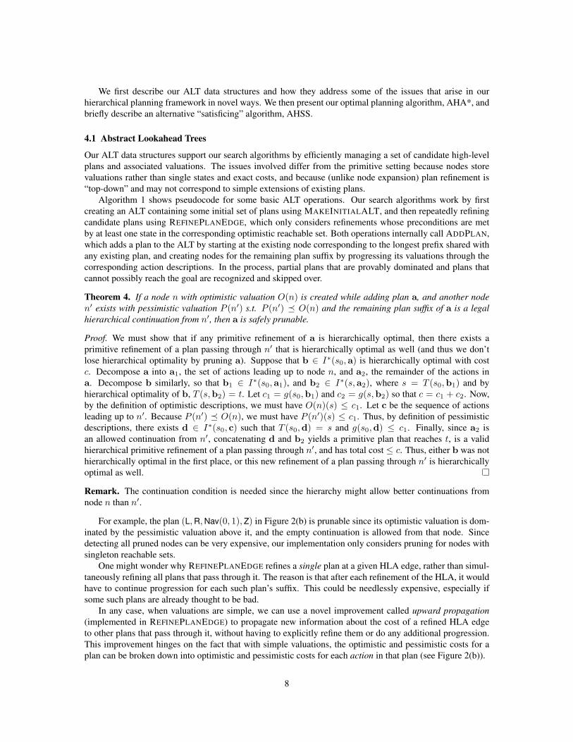
The warehouse world is an elaboration of the well-known blocks world, with discrete spatial constraintsadded. In this domain, a forklift-like gripper hanging from the ceiling can move around and manipulateblocks stacked on a table. Both gripper and blocks occupy single squares in a 2-d grid of allowed positions.The gripper can move to free squares in the four cardinal directions, turn (to face the other way) when in thetop row, and pick up and put down blocks from either side. Each primitive action has unit cost. Becauseof the limited maneuvering space, warehouse world problems can be rather difficult. For instance, Figure 3shows a problem that cannot be solved in fewer than 50 primitive steps. The figure also shows our HLAs forthe domain, which we use unchanged from (MRW ’07) along with the NCSTRIPS descriptions therein (towhich we add simple cost bounds). We consider six instances of varying difficulty.

For the nav-switch domain, we consider square grids of varying size with 3 randomly placed switches,where the goal is always to navigate from one corner to the other. We use the hierarchy and descriptionsdescribed above.

We first present results for our offline algorithms on these domains (see Table 1). On the warehouse worldinstances, nonhierarchical (flat) A* does reasonably well on small problems, but quickly becomes impracticalas the optimal plan length increases. AHA* is able to plan optimally in larger problems, but for the largestinstances, it too runs out of time. The reason is that it must not only find the optimal plan, but also prove thatall other high-level plans have higher cost. In contrast, AHSS with a threshold of ∞ is able to solve all theproblems fairly quickly.

We also included, for comparison, results for the Hierarchical Forward Search (HFS) algorithm (MRW’07), which does not consider plan cost. When passed a threshold of ∞, AHSS has the same objectiveas HFS: to find any plan from s0 to t with as little computation as possible. However, AHSS has severalimportant advantages over HFS. First, its priority function serves as a heuristic, and usually results in higher-quality plans being found. Second, AHSS is actually much simpler. In particular, whereas HFS requirediterative deepening, cycle checking, and a special plan decomposition mechanism to ensure completeness andefficiency, the use of cost information allows AHSS to naturally reap the same benefits without needing anysuch explicit mechanisms. Finally, the abstract lookahead tree data structure provides caching and decreasesthe number of NCSTRIPS progressions required. Due to these improvements, HFS is slightly slower thanthe optimal planner AHA*, and a few orders of magnitude slower than AHSS.

On the nav-switch instances, results are qualitatively similar. Again, flat A* quickly becomes impracticalas the problem size grows. However, in this domain, AHA* actually performs very well, almost matching theperformance of AHSS. The reason is that in this domain, the descriptions for Nav are exact, and thus AHA*can very quickly find a provably optimal high-level plan and refine it down to the primitive level withoutbacktracking, as described earlier.

The obvious next step would be to compare AHA* with other optimal hierarchical planners, such asSHOP2 on its “optimal” setting. However, this is far from straightforward, for several reasons. First, usefulhierarchies are often not optimality-preserving, and it is not at all obvious how we should compare different“optimal” planners that use different standards for optimality. Second, as described in the related work sectionbelow, the type and amount of problem-specific information provided to our algorithms can be very differentthan for HTN planners such as SHOP2. We have yet to find a way to perform meaningful experimentalcomparisons under these circumstances.

For the online setting, we compared (flat) LRTA* and AHLRTA*. The performance of an online algorithmon a given instance depends on the number of allowed refinements per step. Our graphs therefore plot totalcost against refinements per step for LRTA* and AHLRTA*. AHLRTA* took about five times longer perrefinement than LRTA* on average, though this factor could probably be decreased by optimizing the DNFoperations.13

12. Our code and data are available at http://www.cs.berkeley.edu/∼jawolfe/angelic/13. It cannot be completely avoided because refinements for the hierarchical algorithms require multiple progressions.

15

1

1 2

2

3

3

4

4

t1 t2 t3 t4

a b

c

HLA GoalAct Achieve goal by seq. of MovesMove(b, c) Stack block b on c by NavT to

one side of b, pick it up, NavT toone side of c, put b down.

NavT(x, y) Go to (x, y), possibly turningNav(x, y) Go directly to (x, y)

Figure 3: Left: A 4x4 warehouse world problem with goal ON(c, t2) ∧ ON(a, c). Right: HLAs for warehouseworld domain.

nav-switchsz A* AHA* AHSS5 0 0 0

10 22 1 120 176 3 340 – 40 40

warehouse world# A* AHA* AHSS HFS1 1 0 0 12 9 4 2 123 – 63 9 1354 – 526 27 –5 – – 60 –6 – – 48 –

Table 1: Run-times of offline algorithms, rounded to the nearest second, on some nav-switch and warehouseworld problem instances. The algorithms are (flat) graph A*, AHA*, AHSS with threshold α=∞,and HFS from (MRW ’07). Algorithms were terminated if they failed to return within 104 seconds(shown as “–”).

The left graph of Figure 4 is averaged across three instances of the nav-switch world. This domain isrelatively easy as an online lookahead problem, because the Manhattan-distance heuristic for Act alwayspoints in roughly the right direction. In all cases, the hierarchical agent behaved optimally given about 50refinements per step. With this number of refinements, the flat agent usually followed a reasonable, thoughsuboptimal plan. But it did not display optimal behavior, even when the number of refinements per step wasincreased to 1000.

The right graph in Figure 4 shows results averaged across three instances of the warehouse world. Thisdomain is more challenging for online lookahead, as the combinatorial structure of the problem makes the Actheuristic less reliable. AHLRTA* started to behave optimally given a few hundred refinements per step. Incontrast, flat lookahead was very suboptimal (note that the y-axis is on a log scale), even given five thousandrefinements.

Here are some qualitative phenomena we observed on the experiments (data available at paper website).First, as the number of refinements increased, AHLRTA* reached a point where it found a provably optimalprimitive plan on each environment step. But it also had reasonable behavior when the number of refinementsdid not suffice to find a provably optimal plan (the left portion of the right-hand graph), in that the “intended”plan at each step typically consisted of a few primitive actions followed by increasingly high-level actions,and this intended plan was usually reasonable at the high level. Second, when very few refinements (< 50)were allowed per step, AHLRTA* actually did worse than LRTA* on (a single instance of) the nav-switchworld. While we do not completely understand the cause, what seems to be happening is that in the regime ofvery little deliberation time per step, lookahead pathologies and the LRTA* learning rule interact in complexways, often causing the agent to spend long periods of time “filling out” local minima of the heuristic functionin the state space.14 This phenomenon is further complicated in the hierarchical case by the fact that the costbounds for different HLAs tend to be systematically biased in different ways (for example, the optimisticbound for Nav is nearly exact, while the bound for Move tends to underestimate by a factor of two). Improved

14. This is also why the LRTA* curve in the warehouse world is non-monotonic.

16

130

140

150

160

170

180

0 200 400 600 800 1000

tota

l so

luti

on

co

st

refinements per env. step

nav-switch

LRTA*AHLRTA*

10

100

1000

10000

0 1000 2000 3000 4000 5000refinements per env. step

warehouse world

LRTA*AHLRTA*

Figure 4: Total cost-to-goal for online algorithms as a function of the number of allowed refinements per en-vironment step, averaged over three instances each of the nav-switch domain (left) and warehouseworld (right). (Warehouse world costs shown in log-scale.)

online lookahead algorithms that degrade gracefully in such situations, even given very little deliberationtime, are an interesting topic for future work.

7. Related WorkWe briefly describe work related to our specific contributions, deferring to (MRW ’07) for discussion ofrelationships between this general line of work and previous approaches.

Most previous work in hierarchical planning (Tate, 1977; Yang, 1990; Russell and Norvig, 2003) hasviewed HLA descriptions (when used at all) as constraints on the planning process (e.g., “only considerrefinements that achieve p”), rather than as making true assertions about the effects of HLAs. Such HTNplanning systems, e.g., SHOP2 (Nau et al., 2003), have achieved impressive results in previous planningcompetitions and real-world domains—despite the fact that they cannot assure the correctness or bound thecost of abstract plans. Instead, they encode a good deal of domain-specific advice on which refinements totry in which circumstances, often expressed as arbitrary program code. For fairly simple domains describedin tens of lines of PDDL, SHOP2 hierarchies can include hundreds or thousands of lines of Lisp code. Incontrast, our algorithms only require a (typically simple) hierarchical structure, along with descriptions thatlogically follow from (and are potentially automatically derivable from) this structure.

The closest work to ours is by Doan and Haddawy (1995). Their DRIPS planning system uses actionabstraction along with an analogue of our optimistic descriptions to find optimal plans in the probabilisticsetting. However, without pessimistic descriptions, they can only prove that a given high-level plan satisfiessome property when the property holds for all of its refinements, which severely limits the amount of pruningpossible compared to our approach. Helwig and Haddawy (1996) extended DRIPS to the online setting. Theiralgorithm did not cache backed-up values, and hence cannot guarantee eventual goal achievement, but it wasprobably the first principled online hierarchical lookahead agent.

Several other works have pursued similar goals to ours, but using state abstraction rather than HLAs.Holte et al. (1996) developed Hierarchical A*, which uses an automatically constructed hierarchy of stateabstractions in which the results of optimal search at each level define an admissible heuristic for search atthe next-lower level. Similarly, Bulitko et al. (2007) proposed the PR LRTS algorithm, a real-time algorithmin which a plan discovered at each level constrains the planning process at the next-lower level.

Finally, other works have considered adding pessimistic bounds to the A* (Berliner, 1979) and LRTA*(Ishida and Shimbo, 1996) algorithms, to help guide search and exploration as well as monitor convergence.These techniques may also be useful for our corresponding hierarchical algorithms.

17

8. DiscussionWe have presented several new algorithms for hierarchical planning with promising theoretical and empiricalproperties. There are many interesting directions for future work, such as developing better representationsfor descriptions and valuations, automatically synthesizing descriptions from the hierarchy, and generalizingdomain-independent techniques for automatic derivation of planning heuristics to the hierarchical setting.One might also consider extensions to partially ordered, probabilistic, and partially observable settings, andbetter online algorithms that, e.g., maintain more state across environment steps.

9. AcknowledgementsBhaskara Marthi thanks Leslie Kaelbling and Tomas Lozano-Perez for useful discussions. This researchwas also supported by DARPA IPTO, contracts FA8750-05-2-0249 and FA8750-07-D-0185 (subcontract 03-000219).

18

ReferencesH Berliner. The B* Tree Search Algorithm: A Best-First Proof Procedure. Artif. Intell., 12:23–40, 1979.

Vadim Bulitko, Nathan Sturtevant, Jieshan Lu, and Timothy Yau. Graph Abstraction in Real-time HeuristicSearch. JAIR, 30:51–100, 2007.

Tom Bylander. The Computational Complexity of Propositional STRIPS Planning. Artif. Intell., 69:165–204,1994.

A. Doan and P. Haddawy. Decision-theoretic refinement planning: Principles and application. TechnicalReport TR-95-01-01, Univ. of Wisconsin-Milwaukee, 1995.

Richard Fikes and Nils J. Nilsson. STRIPS: A New Approach to the Application of Theorem Proving toProblem Solving. Artif. Intell., 2:189–208, 1971.

James Helwig and Peter Haddawy. An Abstraction-Based Approach to Interleaving Planning and Executionin Partially-Observable Domains. In AAAI Fall Symposium, 1996.

R Holte, M Perez, R Zimmer, and A MacDonald. Hierarchical A*: Searching abstraction hierarchies effi-ciently. In AAAI, 1996.

Toru Ishida and Masashi Shimbo. Improving the learning efficiencies of realtime search. In AAAI, 1996.

Richard E. Korf. Real-Time Heuristic Search. Artif. Intell., 42:189–211, 1990.

Bhaskara Marthi, Stuart J. Russell, and Jason Wolfe. Angelic Semantics for High-Level Actions. In ICAPS,2007.

Drew McDermott. The 1998 AI planning systems competition. AI Magazine, 21(2):35–55, 2000.

Dana Nau, Tsz C. Au, Okhtay Ilghami, Ugur Kuter, William J. Murdock, Dan Wu, and Fusun Yaman.SHOP2: An HTN planning system. JAIR, 20:379–404, 2003.

Ronald Parr and Stuart Russell. Reinforcement Learning with Hierarchies of Machines. In NIPS, 1998.

Stuart Russell and Peter Norvig. Artificial Intelligence: A Modern Approach. Prentice-Hall, EnglewoodCliffs, NJ, 2nd edition, 2003.

A. Tate. Generating project networks. In IJCAI, 1977.

Qiang Yang. Formalizing planning knowledge for hierarchical planning. Comput. Intell., 6(1):12–24, 1990.

19