anguilla australia st. helena & dependencies south georgia & south sandwich islands u.k....
Post on 20-Dec-2015
215 views
TRANSCRIPT

ANGUILLAAUSTRALIA
St. Helena & Dependencies
South Georgia &South Sandwich Islands
U.K.
Serbia & Montenegro(Yugoslavia) FRANCE NIGER INDIA
IRELAND BRAZIL
A Gentle Introduction to Machine Learning A Gentle Introduction to Machine Learning and Data Mining for the Database and Data Mining for the Database
CommunityCommunity
Dr Eamonn KeoghDr Eamonn KeoghUniversity of California - Riverside

Grasshoppers
KatydidsThe Classification ProblemThe Classification Problem(informal definition)
Given a collection of annotated data. In this case 5 instances Katydids of and five of Grasshoppers, decide what type of insect the unlabeled example is.
Katydid or Grasshopper?

Thorax Thorax LengthLength
Abdomen Abdomen LengthLength Antennae Antennae
LengthLength
MandibleMandibleSizeSize
SpiracleDiameter Leg Length
For any domain of interest, we can measure For any domain of interest, we can measure featuresfeatures

Insect Insect IDID
Abdomen Abdomen LengthLength
Antennae Antennae LengthLength
Insect Insect ClassClass
1 2.7 5.5 GrasshopperGrasshopper
2 8.0 9.1 KatydidKatydid
3 0.9 4.7 GrasshopperGrasshopper
4 1.1 3.1 GrasshopperGrasshopper
5 5.4 8.5 KatydidKatydid
6 2.9 1.9 GrasshopperGrasshopper
7 6.1 6.6 KatydidKatydid
8 0.5 1.0 GrasshopperGrasshopper
9 8.3 6.6 KatydidKatydid
10 8.1 4.7 KatydidsKatydids
11 5.1 7.0 ??????????????
We can store features We can store features in a database.in a database.
My_CollectionMy_Collection
The classification The classification problem can now be problem can now be expressed as:expressed as:
• Given a training database Given a training database ((My_CollectionMy_Collection), predict ), predict the the class class label of a label of a previously unseen instancepreviously unseen instance
previously unseen instancepreviously unseen instance = =

An
tenn
a L
engt
hA
nte
nna
Len
gth
10
1 2 3 4 5 6 7 8 9 10
1
2
3
4
5
6
7
8
9
Grasshoppers Katydids
Abdomen LengthAbdomen Length

We will return to the previous slide in two minutes. In the meantime, we are going to play a quick game.
I am going to show you some classification problems which were shown to pigeons!
Let us see if you are as smart as a pigeon!
We will return to the previous slide in two minutes. In the meantime, we are going to play a quick game.
I am going to show you some classification problems which were shown to pigeons!
Let us see if you are as smart as a pigeon!

Examples of class A
3 4
1.5 5
6 8
2.5 5
Examples of class B
5 2.5
5 2
8 3
4.5 3
Pigeon Problem 1

Examples of class A
3 4
1.5 5
6 8
2.5 5
Examples of class B
5 2.5
5 2
8 3
4.5 3
8 1.5
4.5 7
What class is this object?
What class is this object?
What about this one, A or B?
What about this one, A or B?
Pigeon Problem 1

Examples of class A
3 4
1.5 5
6 8
2.5 5
Examples of class B
5 2.5
5 2
8 3
4.5 3
8 1.5
This is a B!This is a B!
Pigeon Problem 1
Here is the rule.If the left bar is smaller than the right bar, it is an A, otherwise it is a B.
Here is the rule.If the left bar is smaller than the right bar, it is an A, otherwise it is a B.

Examples of class A
4 4
5 5
6 6
3 3
Examples of class B
5 2.5
2 5
5 3
2.5 3
8 1.5
7 7
Even I know this oneEven I know this one
Pigeon Problem 2 Oh! This ones hard!Oh! This ones hard!

Examples of class A
4 4
5 5
6 6
3 3
Examples of class B
5 2.5
2 5
5 3
2.5 3
7 7
Pigeon Problem 2
So this one is an A.So this one is an A.
The rule is as follows, if the two bars are equal sizes, it is an A. Otherwise it is a B.
The rule is as follows, if the two bars are equal sizes, it is an A. Otherwise it is a B.
Examples of class A
4 4
1 5
6 3
3 7
Examples of class B
5 6
7 5
4 8
7 7
6 6
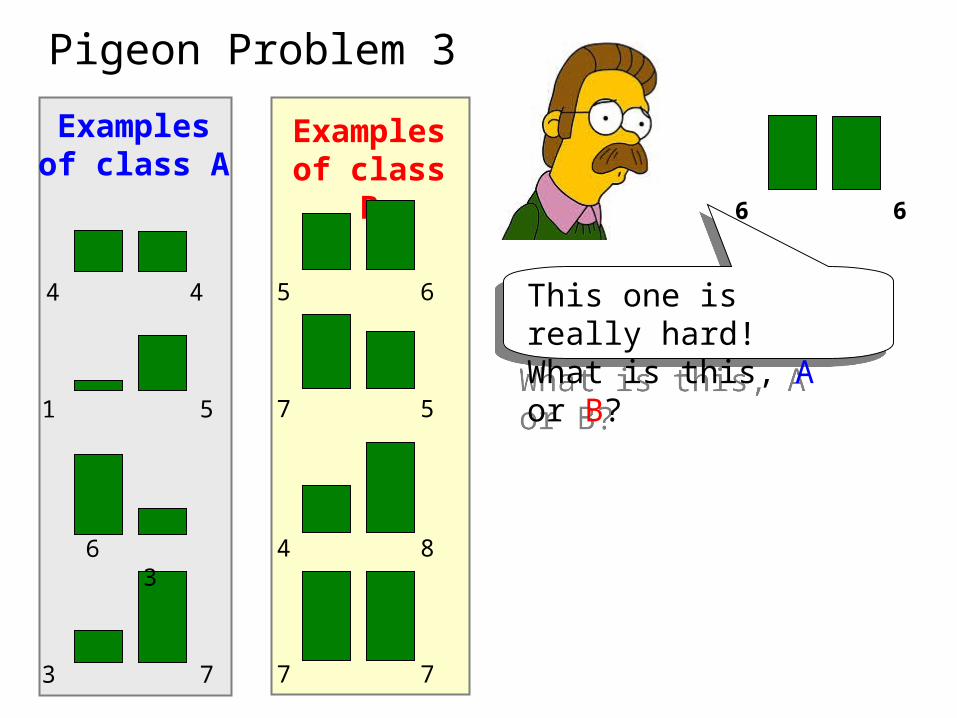
Pigeon Problem 3
This one is really hard!What is this, A or B?
This one is really hard!What is this, A or B?

Examples of class A
4 4
1 5
6 3
3 7
Examples of class B
5 6
7 5
4 8
7 7
6 6
Pigeon Problem 3 It is a B!It is a B!
The rule is as follows, if the square of the sum of the two bars is less than or equal to 100, it is an A. Otherwise it is a B.
The rule is as follows, if the square of the sum of the two bars is less than or equal to 100, it is an A. Otherwise it is a B.

Why did we spend so much time with this game?
Why did we spend so much time with this game?
Because we wanted to show that almost all classification problems have a geometric interpretation, check out the next 3 slides…
Because we wanted to show that almost all classification problems have a geometric interpretation, check out the next 3 slides…
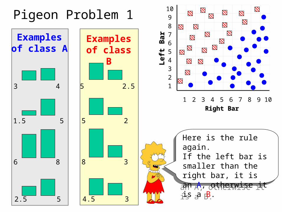
Examples of class A
3 4
1.5 5
6 8
2.5 5
Examples of class B
5 2.5
5 2
8 3
4.5 3
Pigeon Problem 1
Here is the rule again.If the left bar is smaller than the right bar, it is an A, otherwise it is a B.
Here is the rule again.If the left bar is smaller than the right bar, it is an A, otherwise it is a B.
Lef
t B
arL
eft
Bar
10
1 2 3 4 5 6 7 8 9 10
123456789
Right BarRight Bar

Examples of class A
4 4
5 5
6 6
3 3
Examples of class B
5 2.5
2 5
5 3
2.5 3
Pigeon Problem 2
Lef
t B
arL
eft
Bar
10
1 2 3 4 5 6 7 8 9 10
123456789
Right BarRight Bar
Let me look it up… here it is.. the rule is, if the two bars are equal sizes, it is an A. Otherwise it is a B.
Let me look it up… here it is.. the rule is, if the two bars are equal sizes, it is an A. Otherwise it is a B.

Examples of class A
4 4
1 5
6 3
3 7
Examples of class B
5 6
7 5
4 8
7 7
Pigeon Problem 3
Lef
t B
arL
eft
Bar
100
10 20 30 40 50 60 70 80 90 100
102030405060708090
Right BarRight Bar
The rule again:if the square of the sum of the two bars is less than or equal to 100, it is an A. Otherwise it is a B.
The rule again:if the square of the sum of the two bars is less than or equal to 100, it is an A. Otherwise it is a B.

An
tenn
a L
engt
hA
nte
nna
Len
gth
10
1 2 3 4 5 6 7 8 9 10
1
2
3
4
5
6
7
8
9
Grasshoppers Katydids
Abdomen LengthAbdomen Length

An
tenn
a L
engt
hA
nte
nna
Len
gth
10
1 2 3 4 5 6 7 8 9 10
1
2
3
4
5
6
7
8
9
Abdomen LengthAbdomen Length
KatydidsGrasshoppers
• We can “project” the previously unseen instance previously unseen instance into the same space as the database.
• We have now abstracted away the details of our particular problem. It will be much easier to talk about points in space.
• We can “project” the previously unseen instance previously unseen instance into the same space as the database.
• We have now abstracted away the details of our particular problem. It will be much easier to talk about points in space.
11 5.1 7.0 ??????????????previously unseen instancepreviously unseen instance = =

Simple Linear ClassifierSimple Linear Classifier
10
1 2 3 4 5 6 7 8 9 10
1
2
3
4
5
6
7
8
9
If previously unseen instance previously unseen instance above the linethen class is Katydidelse class is Grasshopper
KatydidsGrasshoppers
R.A. Fisher1890-1962


10
1 2 3 4 5 6 7 8 9 10
123456789
100
10 20 30 40 50 60 70 80 90 100
10
20
30
40
50
60
70
80
90
10
1 2 3 4 5 6 7 8 9 10
123456789
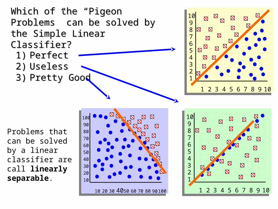
Which of the “Pigeon Problems” can be Which of the “Pigeon Problems” can be solved by the Simple Linear Classifier?solved by the Simple Linear Classifier?
1)1) PerfectPerfect2)2) UselessUseless3)3) Pretty GoodPretty Good
Problems that can be solved by a linear classifier are call linearly separable.

Grasshopper
Antennae shorter than body?
Cricket
Foretiba has ears?
Katydids Camel Cricket
Yes
Yes
Yes
No
No
3 Tarsi?
No
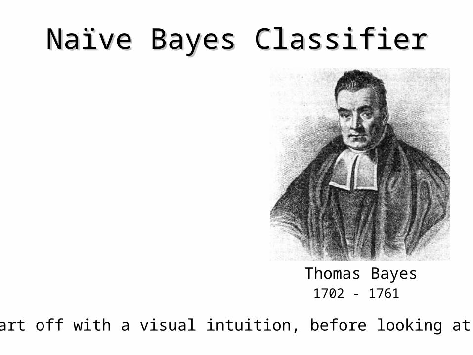
Naïve Bayes ClassifierNaïve Bayes Classifier
We will start off with a visual intuition, before looking at the math…
Thomas Bayes1702 - 1761
An
tenn
a L
engt
hA
nte
nna
Len
gth
10
1 2 3 4 5 6 7 8 9 10
1
2
3
4
5
6
7
8
9
Grasshoppers Katydids
Abdomen LengthAbdomen Length
Remember this example? Remember this example? Let’s get lots more data…Let’s get lots more data…
Remember this example? Remember this example? Let’s get lots more data…Let’s get lots more data…

An
tenn
a L
engt
hA
nte
nna
Len
gth
10
1 2 3 4 5 6 7 8 9 10
1
2
3
4
5
6
7
8
9
KatydidsGrasshoppers
With a lot of data, we can build a histogram. Let us With a lot of data, we can build a histogram. Let us just build one for “Antenna Length” for now…just build one for “Antenna Length” for now…

We can leave the histograms as they are, or we can summarize them with two normal distributions.
Let us us two normal distributions for ease of visualization in the following slides…
p(cj | d) = probability of class cj, given that we have observed dp(cj | d) = probability of class cj, given that we have observed d
3
Antennae length is 3
• We want to classify an insect we have found. Its antennae are 3 units long. How can we classify it?
• We can just ask ourselves, give the distributions of antennae lengths we have seen, is it more probable that our insect is a Grasshopper or a Katydid.• There is a formal way to discuss the most probable classification…
10
2
P(Grasshopper | 3 ) = 10 / (10 + 2) = 0.833
P(Katydid | 3 ) = 2 / (10 + 2) = 0.166
3
Antennae length is 3
p(cj | d) = probability of class cj, given that we have observed dp(cj | d) = probability of class cj, given that we have observed d

9
3
P(Grasshopper | 7 ) = 3 / (3 + 9) = 0.250
P(Katydid | 7 ) = 9 / (3 + 9) = 0.750
7
Antennae length is 7
p(cj | d) = probability of class cj, given that we have observed dp(cj | d) = probability of class cj, given that we have observed d
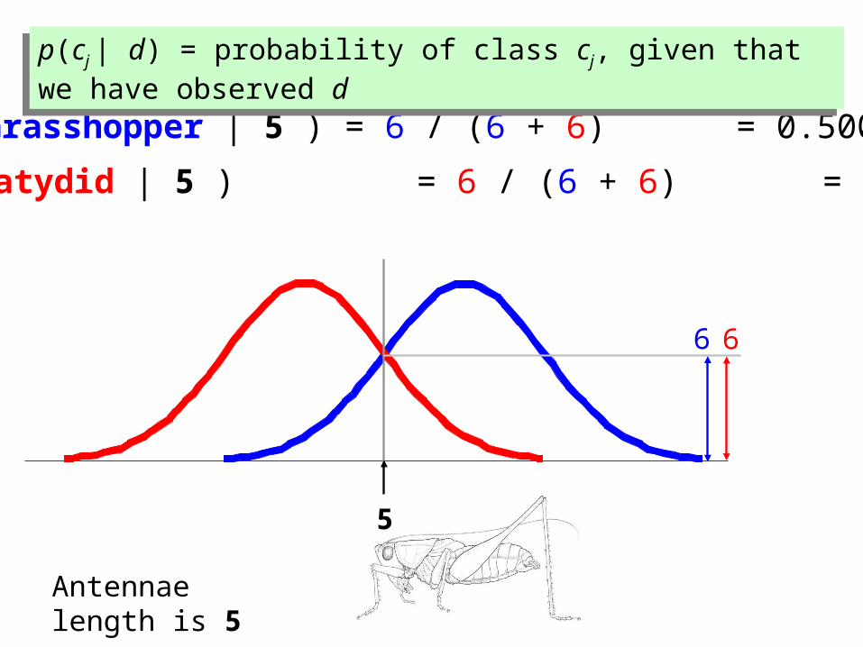
66
P(Grasshopper | 5 ) = 6 / (6 + 6) = 0.500
P(Katydid | 5 ) = 6 / (6 + 6) = 0.500
5
Antennae length is 5
p(cj | d) = probability of class cj, given that we have observed dp(cj | d) = probability of class cj, given that we have observed d
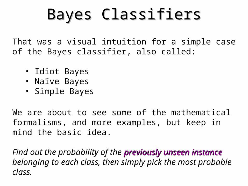
Bayes ClassifiersBayes Classifiers
That was a visual intuition for a simple case of the Bayes classifier, also called:
• Idiot Bayes • Naïve Bayes• Simple Bayes
We are about to see some of the mathematical formalisms, and more examples, but keep in mind the basic idea.
Find out the probability of the previously unseen instance previously unseen instance belonging to each class, then simply pick the most probable class.

Bayes ClassifiersBayes Classifiers• Bayesian classifiers use Bayes theorem, which says
p(cj | d ) = p(d | cj ) p(cj) p(d)
• p(cj | d) = probability of instance d being in class cj, This is what we are trying to compute
• p(d | cj) = probability of generating instance d given class cj,
We can imagine that being in class cj, causes you to have feature d with some probability
• p(cj) = probability of occurrence of class cj,
This is just how frequent the class cj, is in our database
• p(d) = probability of instance d occurring
This can actually be ignored, since it is the same for all classes

Assume that we have two classes
c1 = malemale, and c2 = femalefemale.
We have a person whose sex we do not know, say “drew” or d.
Classifying drew as male or female is equivalent to asking is it more probable that drew is malemale or femalefemale, I.e which is greater p(malemale | drew) or p(femalefemale | drew)
p(malemale | drew) = p(drew | malemale ) p(malemale)
p(drew)
(Note: “Drew can be a male or female name”)
What is the probability of being called “drew” given that you are a male?
What is the probability of being a male?
What is the probability of being named “drew”? (actually irrelevant, since it is that same for all classes)
Drew Carey
Drew Barrymore

p(cj | d) = p(d | cj ) p(cj)
p(d)
Officer Drew
Name Sex
Drew MaleMale
Claudia FemaleFemale
Drew FemaleFemale
Drew FemaleFemale
Alberto MaleMale
Karin FemaleFemale
Nina FemaleFemale
Sergio MaleMale
This is Officer Drew (who arrested me in This is Officer Drew (who arrested me in 1997). Is Officer Drew a 1997). Is Officer Drew a MaleMale or or FemaleFemale??
Luckily, we have a small database with names and sex.
We can use it to apply Bayes rule…

p(malemale | drew) = 1/3 * 3/8 = 0.125
3/8 3/8
p(femalefemale | drew) = 2/5 * 5/8 = 0.250
3/8 3/8
Officer Drew
p(cj | d) = p(d | cj ) p(cj)
p(d)
Name Sex
Drew MaleMale
Claudia FemaleFemale
Drew FemaleFemale
Drew FemaleFemale
Alberto MaleMale
Karin FemaleFemale
Nina FemaleFemale
Sergio MaleMale
Officer Drew is more likely to be a FemaleFemale.

Officer Drew IS a female!Officer Drew IS a female!
Officer Drew
p(malemale | drew) = 1/3 * 3/8 = 0.125
3/8 3/8
p(femalefemale | drew) = 2/5 * 5/8 = 0.250
3/8 3/8

Name Over 170CM Eye Hair length Sex
Drew No Blue Short MaleMale
Claudia Yes Brown Long FemaleFemale
Drew No Blue Long FemaleFemale
Drew No Blue Long FemaleFemale
Alberto Yes Brown Short MaleMale
Karin No Blue Long FemaleFemale
Nina Yes Brown Short FemaleFemale
Sergio Yes Blue Long MaleMale
p(cj | d) = p(d | cj ) p(cj)
p(d)
So far we have only considered Bayes Classification when we have one attribute (the “antennae length”, or the “name”). But we may have many features.How do we use all the features?

• To simplify the task, naïve Bayesian classifiers assume attributes have independent distributions, and thereby estimate
p(d|cj) = p(d1|cj) * p(d2|cj) * ….* p(dn|cj)
The probability of class cj generating instance d, equals….
The probability of class cj generating the observed value for feature 1, multiplied by..
The probability of class cj generating the observed value for feature 2, multiplied by..

• To simplify the task, naïve Bayesian classifiers assume attributes have independent distributions, and thereby estimate
p(d|cj) = p(d1|cj) * p(d2|cj) * ….* p(dn|cj)
p(officer drew|cj) = p(over_170cm = yes|cj) * p(eye =blue|cj) * ….
Officer Drew is blue-eyed, over 170cm tall, and has long hair
p(officer drew| FemaleFemale) = 2/5 * 3/5 * ….
p(officer drew| MaleMale) = 2/3 * 2/3 * ….

p(d1|cj) p(d2|cj) p(dn|cj)
cjThe Naive Bayes classifiers is often represented as this type of graph…
Note the direction of the arrows, which state that each class causes certain features, with a certain probability
…

Naïve Bayes is fast and Naïve Bayes is fast and space efficientspace efficient
We can look up all the probabilities with a single scan of the database and store them in a (small) table…
Sex Over190cm
MaleMale Yes 0.15
No 0.85
FemaleFemale Yes 0.01
No 0.99
cj
…p(d1|cj) p(d2|cj) p(dn|cj)
Sex Long Hair
MaleMale Yes 0.05
No 0.95
FemaleFemale Yes 0.70
No 0.30
Sex
MaleMale
FemaleFemale

Naïve Bayes is NOT sensitive to irrelevant features...Naïve Bayes is NOT sensitive to irrelevant features...
Suppose we are trying to classify a persons sex based on several features, including eye color. (Of course, eye color is completely irrelevant to a persons gender)
p(Jessica | FemaleFemale) = 9,000/10,000 * 9,975/10,000 * ….
p(Jessica | MaleMale) = 9,001/10,000 * 2/10,000 * ….
p(Jessica |cj) = p(eye = brown|cj) * p( wears_dress = yes|cj) * ….
However, this assumes that we have good enough estimates of the probabilities, so the more data the better.
Almost the same!
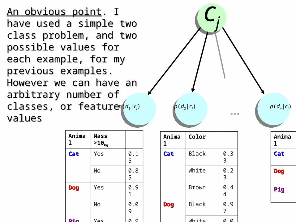
An obvious pointAn obvious point. I have used a . I have used a simple two class problem, and simple two class problem, and two possible values for each two possible values for each example, for my previous example, for my previous examples. However we can have examples. However we can have an arbitrary number of classes, or an arbitrary number of classes, or feature valuesfeature values
Animal Mass >10kg
CatCat Yes 0.15
No 0.85
DogDog Yes 0.91
No 0.09
PigPig Yes 0.99
No 0.01
cj
…p(d1|cj) p(d2|cj) p(dn|cj)
Animal
CatCat
DogDog
PigPig
Animal Color
CatCat Black 0.33
White 0.23
Brown 0.44
DogDog Black 0.97
White 0.03
Brown 0.90
PigPig Black 0.04
White 0.01
Brown 0.95

Naïve Bayesian Naïve Bayesian ClassifierClassifier
p(d1|cj) p(d2|cj) p(dn|cj)
p(d|cj)Problem!
Naïve Bayes assumes independence of features…
Sex Over 6 foot
Male Yes 0.15
No 0.85
Female Yes 0.01
No 0.99
Sex Over 200 pounds
Male Yes 0.11
No 0.80
Female Yes 0.05
No 0.95

Naïve Bayesian Naïve Bayesian ClassifierClassifier
p(d1|cj) p(d2|cj) p(dn|cj)
p(d|cj)Solution
Consider the relationships between attributes…
Sex Over 6 foot
Male Yes 0.15
No 0.85
Female Yes 0.01
No 0.99
Sex Over 200 pounds
Male Yes and Over 6 foot 0.11
No and Over 6 foot 0.59
Yes and NOT Over 6 foot 0.05
No and NOT Over 6 foot 0.35
Female Yes and Over 6 foot 0.01
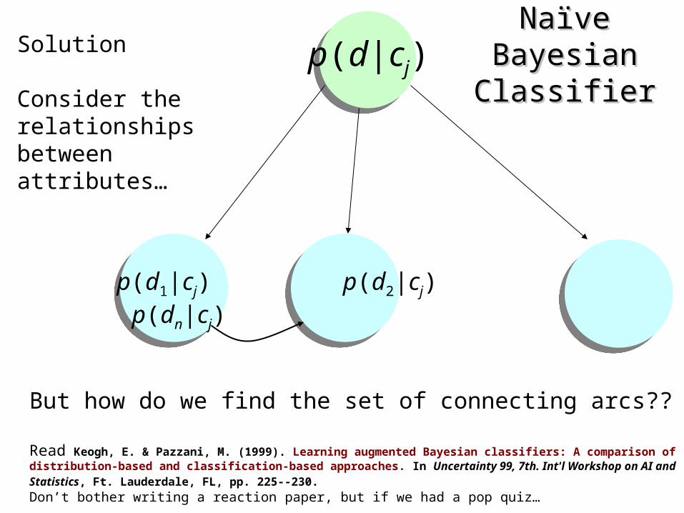
Naïve Bayesian Naïve Bayesian ClassifierClassifier
p(d1|cj) p(d2|cj) p(dn|cj)
p(d|cj)Solution
Consider the relationships between attributes…
But how do we find the set of connecting arcs??
Read Keogh, E. & Pazzani, M. (1999). Learning augmented Bayesian classifiers: A comparison of distribution-based and classification-based approaches. In Uncertainty 99, 7th. Int'l Workshop on AI and Statistics, Ft. Lauderdale, FL, pp. 225--230. Don’t bother writing a reaction paper, but if we had a pop quiz…

Dear SIR,
I am Mr. John Coleman and my sister is Miss Rose Colemen, we are the children of late Chief Paul Colemen from Sierra Leone. I am writing you in absolute confidence primarily to seek your assistance to transfer our cash of twenty one Million Dollars ($21,000.000.00) now in the custody of a private Security trust firm in Europe the money is in trunk boxes deposited and declared as family valuables by my late father as a matter of fact the company does not know the content as money, although my father made them to under stand that the boxes belongs to his foreign partner.…

This mail is probably spam. The original message has been attached along with this report, so you can recognize or block similar unwanted mail in future. See http://spamassassin.org/tag/ for more details.
Content analysis details: (12.20 points, 5 required)NIGERIAN_SUBJECT2 (1.4 points) Subject is indicative of a Nigerian spamFROM_ENDS_IN_NUMS (0.7 points) From: ends in numbersMIME_BOUND_MANY_HEX (2.9 points) Spam tool pattern in MIME boundaryURGENT_BIZ (2.7 points) BODY: Contains urgent matterUS_DOLLARS_3 (1.5 points) BODY: Nigerian scam key phrase ($NN,NNN,NNN.NN)DEAR_SOMETHING (1.8 points) BODY: Contains 'Dear (something)'BAYES_30 (1.6 points) BODY: Bayesian classifier says spam probability is 30 to 40% [score: 0.3728]
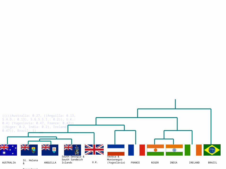
ANGUILLAAUSTRALIA
St. Helena & Dependencies
South Georgia &South Sandwich Islands U.K.
Serbia & Montenegro(Yugoslavia) FRANCE NIGER INDIA IRELAND BRAZIL
(((((Australia: 0.27, ((Anguilla: 0.13, S.H.D.: 0.13), S.G.S.S.I.: 0.2)), U.K.: 0.4) (Yugoslavia: 0.47, France: 0.47)) ((Niger: 0.2, India: 0.2), Ireland: 0.47)), Brazil: 1)

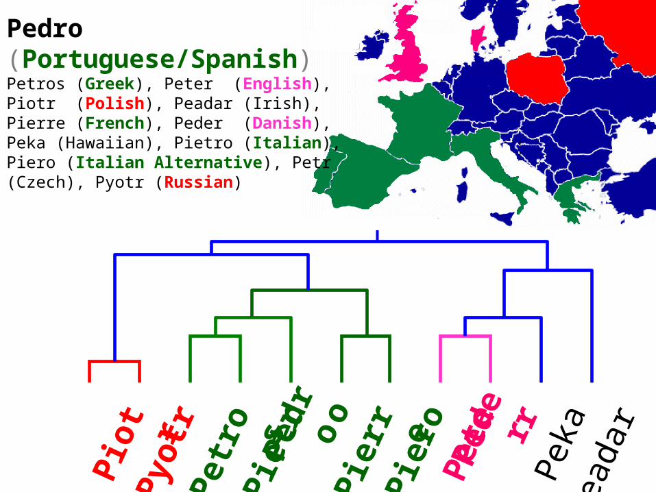
Pedro (Portuguese)Petros (Greek), Peter (English), Piotr (Polish), Peadar (Irish), Pierre (French), Peder (Danish), Peka (Hawaiian), Pietro (Italian), Piero (Italian Alternative), Petr (Czech), Pyotr (Russian)
Cristovao (Portuguese)Christoph (German), Christophe (French), Cristobal (Spanish), Cristoforo (Italian), Kristoffer (Scandinavian), Krystof (Czech), Christopher (English)
Miguel (Portuguese)Michalis (Greek), Michael (English), Mick (Irish!)
A Demonstration of Hierarchical Clustering using String Edit Distance A Demonstration of Hierarchical Clustering using String Edit Distance P
iotr
Pyo
tr P
etro
s P
ietr
oPe
dro
Pie
rre
Pie
ro P
eter
Pede
r P
eka
Pea
dar
Mic
halis
Mic
hael
Mig
uel
Mic
kC
rist
ovao
Chr
isto
pher
Chr
isto
phe
Chr
isto
phC
risd
ean
Cri
stob
alC
rist
ofor
oK
rist
offe
rK
ryst
of
Pio
tr P
yotr
Pet
ros
Pie
tro
Ped
ro P
ierr
e P
iero
Pet
erP
eder
Pek
a P
eada
r
Pedro (Portuguese/Spanish)Petros (Greek), Peter (English), Piotr (Polish), Peadar (Irish), Pierre (French), Peder (Danish), Peka (Hawaiian), Pietro (Italian), Piero (Italian Alternative), Petr (Czech), Pyotr (Russian)