angular momentum & ring/sphere - physics at oregon state

2/26/10 8-1

Chapter 8 Angular Momentum

In the last two chapters we have learned the fundamentals of solving quantum mechanical problems with the wave function approach. We studied free particles and particles bound in idealized square potential energy wells. We are now ready to attack the most important problem in the history of quantum mechanics—the hydrogen atom. The ability to solve this problem and compare it with precision experiments has played a central role in making quantum mechanics the best proven theory in physics.

The hydrogen atom is the bound state of a negatively charged electron and a postively charged proton that are attracted to each other by the Coulomb force. Compared to the problems in the last two chapters, the hydrogen atom system presents us with two primary complications: two particles and three dimensions. The goal of this chapter is to simplify both these aspects of the problem. Similar to the approach taken in classical mechanics, we reduce the two-body problem to a fictitious one-body problem and we separate the three spatial degrees of freedom in a way that each coordinate can be treated independently. In this chapter, we focus on the two angular degrees of freedom because they relate to the angular momentum, which is a conserved quantity. In the next chapter, we solve the radial aspect of the problem, which leads to the quantized energy levels of the hydrogen atom.

As always in quantum mechanics, we begin with Schrödinger's equation

H ! = i!d

dt! . (8.1)

Of course, to use Schrödinger's equation, we must first find the energy eigenstates by solving the energy eigenvalue equation

H E = E E . (8.2)

For a three-dimensional system of two particles, the Hamiltonian is the sum of the kinetic energies of the two individual particles and the potential energy that describes the interaction between them:

H =p1

2

2m1

+p2

2

2m2

+U(r1,r2) (8.3)

Particle 1 has mass m1, position r

1 and momentum p

1, particle 2 has mass m

2, position

r2 and momentum p

2, and the interaction of the two particles is characterized by the

potential energy U(r1,r2) . We assume that the potential energy depends only on the

separation of the particles

U(r1,r2) =U( r

1! r

2) (8.4)

which we refer to as a central potential.

Chap. 8 Angular Momentum

2/26/10

8-2

8.1 Reduced Mass In classical mechanics, we simplify the motion of a system of particles by

separating the motion of the composite system into the motion of the center of mass and the motion about the center of mass. We take this same approach to simplify the quantum mechanical description of the hydrogen atom. As illustrated in Fig. 1, we define the center-of-mass coordinate position vector as

R =m

1r

1+ m

2r

2

m1+ m

2

(8.5)

and the relative position vector as r = r

1! r

2. (8.6)

In classical mechanics, we typically use velocities, which are obtained by differentiation of position with respect to time. In quantum mechanics, we use momentum as the preferred quantity, so the appropriate quantities to separate the two-body motion are the momentum of the center of mass

P = p

1+ p

2 (8.7)

and the relative momentum

p =m

2 p

1! m

1 p

2

m1+ m

2

. (8.8)

The relative momentum takes the simpler form that looks like a relative velocity

p

!=

p1

m1

!p

2

m2

. (8.9)

if we define the reduced mass µ:

Figure 8.1 Center of mass and relative coordinates.


2/26/10

8-3

1

!=

1

m1

+1

m2

! =m

1m

2

m1+ m

2

. (8.10)

With the definitions in Eqns. (8.7) and (8.8), the two-body Hamiltonian in Eqn. (8.3) becomes (HW)

H =P2

2M+p2

2µ+U(r) (8.11)

where the relative particle separation r is the magnitude r1! r

2. We now separate the

Hamiltonian into two independent parts: H = H

CM+ H

rel (8.12)

where the center-of-mass term

HCM

=P2

2M (8.13)

represents the motion of a particle of mass M = m1+ m

2 located at position R with

momentum P = p

1+ p

2, and the relative term

Hrel =p2

2µ+U(r) (8.14)

represents the motion of a single fictitious particle of mass µ located at position r = r

1! r

2 with momentum

p subject to a potential energy U(r) created by an infinitely

massive force center at the origin. Notice that the center-of-mass vector R does not appear in the Hamiltonian, which, classically, is a reflection of the fact that the momentum of the center of mass is conserved because there are no external forces.

The separation of the Hamiltonian into center-of-mass motion and relative motion can also be done using the explicit position representation of the momentum operators as differentials. In the position representation, the one-dimensional momentum operator is

p ! !i"

d

dx (8.15)

In three dimensions, the momentum operator is

p ! !i"""x

i +""y

j+""z

k#$%

&'(= !i") (8.16)

where ! is the gradient operator. For a two-particle system, the momentum operators for the two particles are


2/26/10

8-4

p1! !i"

""x

1

i +""y

1

j+""z

1

k#

$%&

'(= !i")

1

p2! !i"

""x

2

i +""y

2

j+""z

2

k#

$%&

'(= !i")

2

(8.17)

Substituting these position representations into the Hamiltonian in Eqn. (8.3) leads to the same separation as in Eqn. (8.11), where the center-of-mass momentum operator has the position representation (HW)

P ! !i"""X

i +""Y

j+""Z

k#$%

&'(= !i")

R (8.18)

where X, Y, and Z are the Cartesian coordinates of the center-of-mass vector R and !R

is the gradient operator corresponding to the relative coordinates. The relative momentum operator has the position representation

p ! !i"""x

i +""y

j+""z

k#$%

&'(= !i")

r (8.19)

where x, y, and z are the Cartesian coordinates of the relative position vector r = r1! r

2

and !r is the gradient operator corresponding to the relative coordinates. With the Hamiltonian separated into center-of-mass motion and relative motion,

we expect that the quantum state vector can also be separated. This is not always the case, as we saw in the discussion of entanglement in Chap. 4, but it is a valid assumption for the hydrogen atom problem we want to solve. Hence, we write the wave function for the system as

! system R,r( ) =! CM R( )!!! rel r( ) (8.20)

The energy eigenvalue equation for the system is

H!system

R,r( ) = Esystem!!

systemR,r( ) (8.21)

and substituting the separated Hamiltonians (Eqn. (8.12)) and separated wave function (Eqn. (8.20)) gives

HCM + Hrel( )! CM R( )!! rel r( ) = Esystem !! CM R( )!! rel r( ) (8.22)

The separate center-of-mass and relative Hamiltonians act only on their respective wave functions because the gradients !

R and !

r are independent, so we get

! rel r( )HCM! CM R( ) +! CM R( )Hrel! rel r( )!= Esystem !! CM R( )!! rel r( ) (8.23)

We assert that the separate center-of-mass and relative Hamiltonians satisfy their own energy eigenvalue equations (HW)


2/26/10

8-5

H

CM!

CMR( ) = E

CM!

CMR( )

Hrel!

relr( ) = E

rel!

relr( )

(8.24)

and arrive at the energy eigenvalue equation for the system

H!CMR( )!!

relr( ) = E

CM+ E

rel( )! CMR( )!!

relr( ) (8.25)

which demonstrates that the system energy is the additive energy of the two parts Esystem = ECM + Erel . (8.26)

Using the separate Hamiltonians in Eqns. (8.13) and (8.14), the separated energy eigenvalue equations are

P2

2M!

CMR( ) = E

CM!

CMR( ) (8.27)

and

p2

2µ+U r( )

!"#

$%&' rel r( ) = Erel' rel r( ) (8.28)

The center-of-mass energy eigenvalue equation (8.27) is the free particle eigenvalue equation we encountered in Chap. 6, while the relative motion energy eigenvalue equation (8.28) contains the interaction potential and so has the interesting physics of the hydrogen atom. Using the position representation of the momentum operator in Eqn. (8.18), the center-of-mass energy eigenvalue equation is

!!2

2M

"2

"X 2+

"2

"Y 2+

"2

"Z 2#$%

&'()

CMX,Y ,Z( ) = E

CM)

CMX,Y ,Z( ) (8.29)

The solution to Eqn. (8.29) is the three-dimensional extension of the free-particle eigenstates we studied in Chap. 6

!CM

( X ,Y ,Z ) =1

2"( )3 2

ei P

XX +P

YY+P

ZZ( )/! (8.30)

with energy eigenvalues

ECM

=1

2MPX

2+ P

Y

2+ P

Z

2( ) (8.31)

For measurements of observables associated with the relative motion, the center-of mass wave function contributes only an overall phase to the system wave function and so has no effect on clacuating probabilities of relative motion quantities. We can therefore ignore the center-of-mass motion and concentrate only on the relative motion dictated by the energy eigenvalue equation (8.28). That is the problem we want to solve for the hydrogen atom.


2/26/10

8-6

8.2 Energy Eigenvalue Equation In Spherical Coordinates The relative motion Hamiltonian that governs the hydrogen atom is

H =p2

2µ+U r( ) (8.32)

Using the position representation of the momentum operator in Eqn. (8.19), the Hamiltonian is

H ! !"

2

2µ"

2+U (r) (8.33)

and the energy eigenvalue equation is

!!

2

2µ"2 +U (r)

#

$%&

'() r( ) = E) r( ) (8.34)

where we drop the subscript on the energy and the gradient because we are ignoring the center-of-mass motion the rest of the way.

Because the potential energy in Eqn. (8.34) depends on the parameter r only, this problem is clearly asking for the use of spherical coordinates, centered at the origin of the central force. The system of spherical coordinates is shown in Fig. 2 and the relation between the spherical coordinates r, ! , ! and the Cartesian coordinates x, y, z are

x = r sin! cos"

y = r sin! sin"

z = r cos!

(8.35)

In spherical coordinates, the gradient operator is

! = r"

"r+ #

1

r

"

"#+ $

1

r sin#

"

"$ (8.36)

and the Laplacian operator !2 is:

Figure 8.2 Spherical coordinates.


2/26/10

8-7

!2=

1

r2

""r

r2 ""r

#$%

&'(+

1

r2sin)

"")

sin)"")

#$%

&'(+

1

r2sin

2)"2

"* 2 (8.37)

Using this spherical coordinate representation, the energy eigenvalue equation (8.34) becomes the differential equation

!!

2

2µ

1

r2

""r

r2 ""r

#$%

&'(+

1

r2 sin)

"")

sin)"")

#$%

&'(+

1

r2 sin2)

"2

"* 2

+

,-

.

/01 r,) ,*( )

+U (r)1 r,) ,*( ) = E1 r,) ,*( ) (8.38)

Solving this equation is our primary task, but first let's discuss the important role that angular momentum plays in this equation.

8.3 Angular Momentum

8.3.1 Classical Angular Momentum The classical angular momentum is defined as

L= r!p . (8.39)

In the case of central forces, the torque r ! F is zero and angular momentum is a

conserved quantity:

! =dL

dt= 0 " L=constant (8.40)

A central force F(r) depends only on the distance of the reduced mass from the center of force (i.e., the separation of the two particles) and not on the angular orientation of the sytem. Therefore, the system is spherically symmetric; it is invariant (unchanged) under rotations. Noether's theorem states that whenever the laws of physics are invariant under a particular motion or other operation, there will be a corresponding conserved quantity. In this case, the conservation of angular momentum is related to the invariance of the physical system under rotations.

8.3.2 Quantum Mechanical Angular Momentum In quantum mechanics, the Cartesian components of the angular momentum

operator L= r ! p are represented in the position representation as

Lx

= ypz! zp

y! !i" y

""z

! z""y

#$%

&'(

Ly

= zpx! xp

z! !i" z

""x

! x""z

#$%

&'(

Lz

= xpy! yp

x! !i" x

""y

! y""x

#$%

&'(

(8.41)


2/26/10

8-8

Position and momentum operators for a given axis do not commute ( x, p

x[ ] = i! , etc.), so we might expect that to affect the commutation of angular momentum operators. Position and momentum operators for different axes do commute ( x, p

y!" #$ = 0 , etc.), so

one angular momentum commutator is

Lx, L

y!"

#$ = yp

z% zp

y, zp

x% xp

z!"

#$

= ypz, zp

x!" #$ % yp

z,xp

z!" #$ % zp

y, zp

x!"

#$ + zp

y,xp

z!"

#$

= y pz, z!" #$ p

x% y,x!" #$ p

z% z p

y, p

x!"

#$ + p

yz, p

z!" #$ x

= i! xpy% yp

x( )= i!L

z

(8.42)

Including the cyclic permutations, we arive at the three commutation relations

[Lx, L

y] = i!L

z

[Ly, L

z] = i!L

x

[Lz, L

x] = i!L

y

(8.43)

These are exactly the same commutation relations that spin angular momentum obeys! So orbital and spin angular momentum appear to have something in common, as you might expect.

When we studied spin, we also found it useful to consider the S2 = SiS operator. The corresponding operator for orbital angular momentum is

L

2= LiL= L

x

2+ L

y

2+ L

z

2 (8.44)

In the spin case, the operator S2 commutes with all three component operators. Let's try the same with orbital angular momentum. For example,

L2, L

x!"

#$ = L

x

2+ L

y

2+ L

z

2, L

x!"

#$

= Lx

2, L

x!"

#$ + L

y

2, L

x!"

#$ + L

z

2, L

x!"

#$

= Ly

Ly, L

x!"

#$ + L

y, L

x!"

#$ L

y+ L

zL

z, L

x!" #$ + L

z, L

x!" #$ L

z

= %i!LyL

z% i!L

zL

y+ i!L

zL

y+ i!L

yL

z

= 0

(8.45)

The other two components also commute with L2 :

L2, L

x!"

#$ = 0

L2, L

y!"

#$ = 0

L2, L

z!"

#$ = 0

(8.46)


2/26/10

8-9

So orbital and spin angular momentum obey all the same commutation relations. Though we did not do it that way in Chap. 1, the eigenstates sm

s of spin angular

momentum can be derived solely from the commutation relations of the operators. The spin eigenvalue equations are

S2sm

s= s(s +1)!

2sm

s

Szsm

s= m

s! sm

s

(8.47)

The states sms

are simultaneously eigenstates of S2 and Sz, which is possible because

the two operator commute with each other. Because orbital angular momentum obeys the same commutation relations as spin, the eigenvalue equations for L2 and L

z have the

same form:

L2!m!= !(! +1)"

2!m!

Lz!m!= m

!" !m

!

(8.48)

and we can therefore draw on all the work we did in the spins chapters to help us understand orbital angular momentum. The quantum number ! is the orbital angular momentum quantum number and the quantum number

m! is the orbital magnetic

quantum number. There is one crucial difference between spin angular momentum and orbital

angular momentum. In the spin case, the allowed quantized values of the spin angular momentum quantum number s are the integers and half integers:

s = 0, 1

2,1, 3

2,2, 5

2, 3, 7

2, 4,… (8.49)

In Chaps. 1-3 we studied spin ½ and spin 1 systems. In the case of orbital angular momentum, the quantum number ! is allowed to take on only integer values

! = 0,1,2,3,4,… (8.50)

Other than this important distinction, spin and orbital angular momentum behave the same in quantum mechanical calculations of probabilities, expectation values, etc. The magnetic quantum numbers m

s and

m! span the ranges from !s" +s and !!" +! ,

respectively, in integer steps. In the spin ½ system, we represent the spin operators as matrices:

S2!3

4"2 1 0

0 1

!

"#$

%&!!!!Sz !

"

2

1 0

0 '1!

"#$

%&

Sx !"

2

0 1

1 0

!

"#$

%&!Sy !

"

2

0 'ii 0

!

"#$

%&

(8.51)

where the basis states of the representation are the eigenstates of the S2 and Sz defined in

Eqn. (8.47). For orbital angular momentum, we can also represent the operators as matrices, with the exception that only integer values of ! are allowed. For example, the matrix representations of the orbital angular momentum operators for ! = 1 are


2/26/10

8-10

L2! 2"

2

1 0 0

0 1 0

0 0 1

!

"

##

$

%

&&!!!!!!!!!L

z! "

1 0 0

0 0 0

0 0 '1

!

"

##

$

%

&&

Lx!"

2

0 1 0

1 0 1

0 1 0

!

"

##

$

%

&&

!!!!Ly!"

2

0 'i 0

i 0 'i0 i 0

!

"

##

$

%

&&

(8.52)

where the basis states of the representation are the eigenstates of the L2 and Lz defined

in Eqn. (8.48). These matrices are exactly the same as the spin-1 matrices we defined in Chap. 2.7.

Example 8.1

A particle with orbital angular momentum ! = 1 is in the state

! =

1

3! = 1,m

!= 1 +

2

3! = 1,m

!= 0 . (8.53)

Find the probability that a measurement of Lz will yield the value ! for this state and

calculate the expectation value of Lz?

The eigenstate of Lz with eigenvalue

Lz= +! is

! = 1,m

!= 1 = 11 , so the

probability of measuring Lz= +! is

!!= 11!

2

= 111

311 + 2

310( )

2

= 1

311 11 + 2

311 10

2

(8.54)

the states !m!

form an orthonormal basis, so 11 11 = 1 and 11 10 = 0 , and the probability is

!!=

1

3

2

=1

3

(8.55)

The expectation value of Lz is

Lz= ! L

z! (8.56)

Let's calculate this with matrices. Using the matrix (column) representation of !

! !1

3

1

2

0

"

#

$$

%

&

''

(8.57)

we get


2/26/10

8-11

Lz=1

31 2 0( )!

1 0 0

0 0 0

0 0 !1

"

#

$$

%

&

''1

3

1

2

0

"

#

$$

%

&

''

=!

31 2 0( )

1

0

0

"

#

$$

%

&

''

=!

3

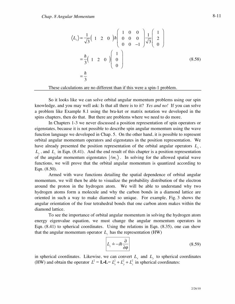
(8.58)

These calculations are no different than if this were a spin-1 problem. So it looks like we can solve orbital angular momentum problems using our spin

knowledge, and you may well ask: Is that all there is to it? Yes and no! If you can solve a problem like Example 8.1 using the bra-ket or matrix notation we developed in the spins chapters, then do that. But there are problems where we need to do more.

In Chapters 1-3 we never discussed a position representation of spin operators or eigenstates, because it is not possible to describe spin angular momentum using the wave function language we developed in Chap. 5. On the other hand, it is possible to represent orbital angular momentum operators and eigenstates in the position representation. We have already presented the position representation of the orbital angular operators L

x,

Ly , and L

z in Eqn. (8.41). And the end result of this chapter is a position representation

of the angular momentum eigenstates !m!

. In solving for the allowed spatial wave functions, we will prove that the orbital angular momentum is quantized according to Eqn. (8.50).

Armed with wave functions detailing the spatial dependence of orbital angular momentum, we will then be able to visualize the probability distribution of the electron around the proton in the hydrogen atom. We will be able to understand why two hydrogen atoms form a molecule and why the carbon bonds in a diamond lattice are oriented in such a way to make diamond so unique. For example, Fig. 3 shows the angular orientation of the four tetrahedral bonds that one carbon atom makes within the diamond lattice.

To see the importance of orbital angular momentum in solving the hydrogen atom energy eigenvalue equation, we must change the angular momentum operators in Eqn. (8.41) to spherical coordinates. Using the relations in Eqn. (8.35), one can show that the angular momentum operator L

z has the representation (HW)

Lz! !i"

"

"# (8.59)

in spherical coordinates. Likewise, we can convert Lx and Ly to spherical coordinates

(HW) and obtain the operator L

2= LiL= L

x

2+ L

y

2+ L

z

2 in spherical coordinates:


2/26/10

8-12

Figure 8.3 Angular dependence of sp3 hybrid orbitals in diamond lattice.

L2! !"2 1

sin"##"

sin"##"

$%&

'()+

1

sin2"

#2

#* 2

+

,-

.

/0 (8.60)

These are the two operators we need to express the angular momentum eigenvalue equations (8.48) in the position representation, which we do later in this chapter.

Now compare the L2 operator in Eqn. (8.60) with the energy eigenvalue equation (8.38). You notice that the L2 operator is part of the differential operator in the energy eigenvalue equation. Hence we can rewrite the energy eigenvalue equation with the L2 operator

!!

2

2µ

1

r2

""r

r2 ""r

#$%

&'(!

1

!2r

2L

2)

*+

,

-./ r,0 ,1( ) +U (r)/ r,0 ,1( ) = E/ r,0 ,1( ) (8.61)

All of the angular part of the Hamiltonian is contained in the angular momentum operator.

8.4 Separation Of Variables We have already simplified the two-body nature of the hydrogen atom problem to

an effective one body problem by separating the relative motion (interesting) from the center-of-mass motion (not so interesting). We now proceed to simplify the three-dimensional aspect of the problem by separating the three spherical coordinate dimensions from each other. To do this, we apply the standard technique of separation of variables to the energy eigenvalue differential equation (8.61). This technique is reviewed in Appendix C, where six steps detail the process in its general form. We apply these steps here to isolate the radial r dependence and the angular

! ," dependence into

separate equations. Step 1: Write the partial differential equation in the appropriate coordinate

system. We have done this already in Eqn. (8.61) above


2/26/10

8-13

!!

2

2µ

1

r2

""r

r2 ""r

#$%

&'(!

1

!2r

2L

2)

*+

,

-./ r,0 ,1( ) +U (r)/ r,0 ,1( ) = E/ r,0 ,1( ) (8.62)

Step 2: Assume that the solution ! r," ,#( ) can be written as the product of

functions, at least one of which depends on only one variable, in this case r . The other function(s) must not depend at all on this variable, i.e., assume

! (r," ,#) = R(r)Y (" ,#) (8.63)

Plug this assumed solution into the partial differential equation (8.62) from step 1. Because of the special form of ! , the partial derivatives each act on only one of the factors in ! . Any partial derivatives that act only on a function of a single variable may be rewritten as total derivatives, yielding

!!

2

2µY

1

r2

d

drr

2 dR

dr

"#$

%&'!

1

!2r

2R(L

2Y )

(

)*

+

,- +U (r)RY = ERY (8.64)

Note that the orbital angular momentum operator L2 acts only on angular spatial functions.

Step 3: Divide both sides of the equation by ! = RY .

!!

2

2µ

1

R

1

r2

d

drr

2 dR

dr

"#$

%&'!

1

Y

1

!2r

2(L

2Y )

(

)*

+

,- +U (r) = E (8.65)

Step 4: Isolate all of the dependence on one coordinate on one side of the equation. To isolate the r dependence we must first clear the r dependence from the angular term (involving angular derivatives in L2 and angular functions in Y ). To do this, we multiply Eqn. (8.65) by r 2 to clear this factor out of the denominators of the angular pieces. Further rearranging Eqn. (8.65) to get all of the r dependence on the right-hand side, we obtain:

1

!2

1

Y ! ,"( )L2Y ! ,"( )

function of ! ," only

" #$$$ %$$$

=1

R r( )d

drr 2

dR r( )dr

#

$%

&

'( )

2µ

!2(E )U (r))r 2

function of r only

" #$$$$$$$ %$$$$$$$

(8.66)

Step 5: Now imagine changing the isolated variable r by a small amount. In principle, the right-hand side of Eqn. (8.66) could change, but nothing on the left-hand side would. Therefore, if the equation is to be true for all values of r , the particular combination of r dependence on the right-hand side must be constant. We can thus define a separation constant, which we call A in this case.

1

!2

1

Y ! ,"( )L

2Y ! ,"( ) =

1

R r( )d

drr

2dR r( )

dr

#

$%

&

'( )

2µ

!2

(E )U (r))r 2 * A (8.67)


2/26/10

8-14

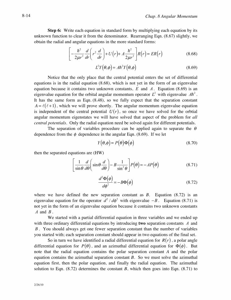
Step 6: Write each equation in standard form by multiplying each equation by its unknown function to clear it from the denominator. Rearranging Eqn. (8.67) slightly, we obtain the radial and angular equations in the more standard forms:

!!

2

2µr2

d

drr

2d

dr

"#$

%&'+U r( )+ A

!2

2µr2

(

)*

+

,-R r( ) = ER r( ) (8.68)

L

2Y ! ,"( ) = A!

2Y ! ,"( ) (8.69)

Notice that the only place that the central potential enters the set of differential equations is in the radial equation (8.68), which is not yet in the form of an eigenvalue equation because it contains two unknown constants, E and A . Equation (8.69) is an eigenvalue equation for the orbital angular momentum operator L2 with eigenvalue A!2 . It has the same form as Eqn. (8.48), so we fully expect that the separation constant

A = ! ! +1( ) , which we will prove shortly. The angular momentum eigenvalue equation is independent of the central potential U r( ) , so once we have solved for the orbtial angular momentum eigenstates we will have solved that aspect of the problem for all central potentials. Only the radial equation need be solved again for different potentials.

The separation of variables procedure can be applied again to separate the ! dependence from the ! dependence in the angular Eqn. (8.69). If we let

Y ! ,"( ) = P !( )# "( ) (8.70)

then the separated equations are (HW)

1

sin!d

d!sin!

d

d!"#$

%&'( B

1

sin2!

)

*+

,

-.P !( ) = (AP !( ) (8.71)

d2! "( )d" 2

= #B! "( ) (8.72)

where we have defined the new separation constant as B. Equation (8.72) is an eigenvalue equation for the operator

d

2/ d! 2 with eigenvalue !B . Equation (8.71) is

not yet in the form of an eigenvalue equation because it contains two unknown constants A and B .

We started with a partial differential equation in three variables and we ended up with three ordinary differential equations by introducing two separation constants A and B . You should always get one fewer separation constant than the number of variables you started with; each separation constant should appear in two equations of the final set.

So in turn we have identified a radial differential equation for R r( ) , a polar angle differential equation for P !( ) , and an azimuthal differential equation for ! "( ) . But note that the radial equation contains the polar separation constant A and the polar equation contains the azimuthal separation constant B. So we must solve the azimuthal equation first, then the polar equation, and finally the radial equation. The azimuthal solution to Eqn. (8.72) determines the constant B, which then goes into Eqn. (8.71) to


2/26/10

8-15

determine the polar angle solution and the constant A. The combined azimuthal and polar solutions also satisfy the eigenvalue Eqn. (8.69) for the orbital angular momentum operator L2 . Finally, the constant A goes into the radial Eqn. (8.68) and the energy eigenvalues are determined. To place these three eigenvalue equations in context we will solve them in order by identifying physical situations that isolate the different equations. In this chapter, we focus on the two angular equations, which are independent of the central potential energy U r( ) . In the next chapter, we solve the radial equation for the special case of the hydrogen atom with the Coulomb potential energy function.

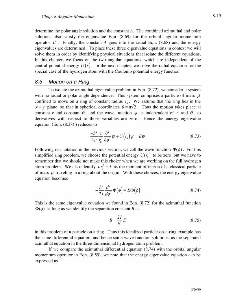
8.5 Motion on a Ring To isolate the azimuthal eigenvalue problem in Eqn. (8.72), we consider a system

with no radial or polar angle dependence. This system comprises a particle of mass µ confined to move on a ring of constant radius

r

0. We assume that the ring lies in the

x ! y plane, so that in spherical coordinates ! = " 2 . Thus the motion takes place at

constant r and constant ! , and the wave function ! is independent of r and ! , so derivatives with respect to those variables are zero. Hence the energy eigenvalue equation (Eqn. (8.38) ) reduces to

!!2

2!

1

r0

2

"2

"# 2$ +U r

0( )$ = E$ (8.73)

Following our notation in the previous section, we call the wave function !(") . For this simplified ring problem, we choose the potential energy

U (r

0) to be zero, but we have to

remember that we should not make this choice when we are working on the full hydrogen atom problem. We also identify

µr

0

2= I as the moment of inertia of a classical particle

of mass µ traveling in a ring about the origin. With these choices, the energy eigenvalue equation becomes

!!

2

2I

d2

d" 2# "( ) = E# "( ) (8.74)

This is the same eigenvalue equation we found in Eqn. (8.72) for the azimuthal function !(") as long as we identify the separation constant B as

B =2I

!2

E (8.75)

in this problem of a particle on a ring. Thus this idealized particle-on-a-ring example has the same differential equation, and hence same wave function solutions, as the separated azimuthal equation in the three-dimensional hydrogen atom problem.

If we compare the azimuthal differential equation (8.74) with the orbital angular momentum operator in Eqn. (8.59), we note that the energy eigenvalue equation can be expressed as


2/26/10

8-16

Lz

2

2I! "( ) = E! "( ) (8.76)

which emphasizes the importance of angular momentum again. This is what you would expect for a classical particle rotating in a circular path in the x ! y plane with kinetic energy

T = 1

2I!

2= L

z

22I and resultant Hamiltonian

H = T =L

z

2

2I (8.77)

assuming no potential energy. We noted earlier that eigenstates of L

z obey an

eigenvalue equation

L

z| m! = m!| m! (8.78)

where we suppress the ! quantum number (for the mopment) because it is not applicable to this idealized one-dimensional particle-on-a-ring problem. The m states are also eigenstates of

L

z

2 :

L

z

2m = m

2!

2m (8.79)

and hence of the Hamiltonian of the particle on a ring:

H m = E m

Lz

2

2Im =

m2!

2

2Im

(8.80)

So it looks like we already know the answer; that the energy eigenvalues are

E = m

2!22I and the separation constant is B = m

2 . However, we know the properties of the m states in the abstract only, we do not know their spatial representation. That comes from solving the differential equation (8.74), which is the position representation of the abstract equation (8.80). Let’s solve it and in so doing confirm our expectations about the energy eigenvalues.

8.5.1 Azimuthal Solution The azimuthal differential equation written in terms of the separation constant is

d2! "( )d" 2

= #B! "( ) (8.81)

The solutions are the complex exponentials

!

m(") = N e

im" (8.82)

where

m = ± B (8.83)


2/26/10

8-17

and N is the normalization constant. There is no "boundary" on the ring, so we cannot impose boundary conditions like

we did for the potenial energy well problems in Chap. 5. However, there is one very important property of the wave function that we can invoke: it must be single-valued. The variable ! is the azimuthal angle around the ring, so that

! + 2" is physically the same

point as ! . If we go once around the ring and return to our starting point, the value of the wave function must remain the same. Therefore the solutions must satisfy the periodicity condition

!

m(" + 2# ) = !

m(") . In order for the eigenstate wave function

!

m(") to be

periodic, the value of m must be real (complex m would result in real exponential solutions. Furthermore, the solutions must have the correct period, which requires that m be an integer:

m = 0,±1,±2,… (8.84)

The quantum number m is called the magnetic quantum number as we saw in the spin problem. Note that the solution permits both positive and negative values of m as well as zero. As expected, we have found that the energy eigenstates for the particle on a ring are the states m that satisfy the L

z eigenvalue equation (8.78).

As usual, we find the normalization constant N in Eqn. (8.82) by requiring that the probability of finding the particle somewhere on the ring is unity:

1=

0

2!

" #m

* ($)#m

($)d$ =0

2!

" N*e% im$

Neim$

d$ = 2! | N |2 (8.85)

We are free to choose the constant to be real and positive:

N =1

2!

(8.86)

We have thus found the spatial representation of the m states:

m ! !m

(") =1

2#e

im" (8.87)

The eigenfunctions of the ring form an orthonormal set:

0

2!

" #k

* ($)#m

($)d$ = %km

(8.88)

The allowed values of the separation constant B are B = m2 , so the possible

energy eigenvalues using Eqn. (8.75) are

Em=!

2

2Im

2 (8.89)

which is exactly what we expected from Eqn. (8.80). The spectrum of allowed energies is shown in Fig. 4. The eigenstates corresponding to + | m | and ! | m | states have the same energy, so this system is degenerate. The ±m degeneracy of the energy eigenstates


2/26/10

8-18

Figure 8.4 Energy spectrum for particle on a ring.

corresponds to

L

z= +m! and

L

z= !m! . That is, the two degenerate states represent

states with opposite components of the angular momentum along the z-axis.

8.5.2 Quantum Measurements on a Particle Confined to a Ring Many of the aspects of quantum meaurement applied to this new system are

similar to the spin and particle-in-a-box examples we have done previously (e.g., Examples 2.3, 5.4, and 8.1. However, the degeneracy of energy levels presents a new aspect. Because the states m and !m have the same energy, the probability of measuring the energy E

m is the sum

!

Em

= m !2

+ "m !2

(8.90)

On the other hand, the state m uniquely specifies the orbtial angular momentum component along the z-direction, so the probability of measuring the angular momentum component is

!

Lz=m!

= m !2

(8.91)

Consider a particle on a ring in the superposition state

! =1

70 + 2 1 + "1 + 2( ) (8.92)

If we measure the energy, then the probability of measuring the value E1= !

22I is


2/26/10

8-19

!E

1

= 1!2

+ "1!2

= 11

70 + 2 1 + "1 + 2( )

2

+ "11

70 + 2 1 + "1 + 2( )

2

= 2

7

2

+ 1

7

2

= 5

7

(8.93)

After the measurement, the new state vector is the normalized projection of the input state onto the kets corresponding to the result of the measurement (Postulate 5, Chap. 2):

!after E

m

=m m + "m "m

!E

m

! (8.94)

which in this case is

!after E

m

=1 1 + "1 "1

!E

m

1

7

0 + 2 1 + "1 + 2( )

=1

5

2 1 + "1( )

(8.95)

A measurement of the angular momentum component L

z after the energy

measurement can be made with a Stern-Gerlach device, and would yield the results shown in Fig. 5. (HW)

8.5.3 Spatial wave function This is a one-dimensional problem, like the problem of a particle-in-a-box we

solved in the Chap. 5 (now in ! instead of x ) and the solutions have the same oscillatory form. As in that problem, the energy eigenvalues are discrete because of a boundary condition. The difference is that the boundary condition appropriate to this problem is periodicity because ! is a physical angle, rather than ! (x) = 0 at the boundaries, appropriate to an infinite potential.

Figure 8.5 Energy measurement and orbital angular momentum measurement.


2/26/10

8-20

The eigenstate wave functions for the partcile on a ring are complex, so we must plot both the real and imaginary components in orde to properly represent the wave function. Plots of three !

m"( ) eigenstates are shown in Fig. 6. The probability density

of the states is

!m!( ) = "

m!( )

2 (8.96)

Substituting in the eigenstate wave functions from Eqn. (8.87)

!m!( ) =

1

2"eim!

2

=1

2" (8.97)

which is a constant independent of the quantum number m. So there is no measurable spatial dependence of the m eigenstates.

However, there is spatial dependence in the probability density for superposition states. For example, consider a state of the system with an initial wave function comprising two eigenstates:

! (",0) = c

1#

m1

(") + c2e

i$#m

2

(") (8.98)

We assume that the function is already properly normalized (so that c

1

2+ c

2

2= 1 ), and we

assume that the constants c1 and c2 are real. An overall phase has no physical meaning (cannot be measured), so we can always choose one coefficient to be real. Relative phases play a crucial role in measurement, so we have made the relative phase explicit by separating the phase ei! from the coefficient of the second term. Using the Schrödinger time evolution recipe from Chap. 3, the time-evolved state of the intial state in Eqn. (8.98) is

! (",t) = c1#

m1

(")e$iE

m1t !

+ c2e

i%#m

2

(")e$iE

m2t !

= c1

1

2&e

im1"e$iE

m1t !

+ c2e

i% 1

2&e

im2"e$iE

m2t !

(8.99)

The location of the particle on the ring is specified by the probability density:

Figure 8.6 Eigenstate wave functions for a particle on a ring. Real part of wave function is solid line and

imaginary part is dashed line.


2/26/10

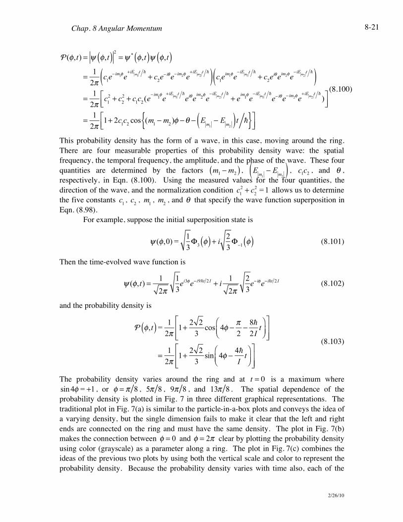
8-21

!(!,t) = " !,t( )2

=" * !,t( )" !,t( )

=1

2#c

1e$ im

1!e+iE

m1t !

+ c2e$ i%

e$ im

2!e+iE

m2t !( ) c

1e

im1!e$iE

m1t !

+ c2e

i%e

im2!e$iE

m2t !( )

=1

2#c

1

2+ c

2

2+ c

1c

2(e

$ im1!e+iE

m1t !

ei%

eim

2!e$iE

m2t !

+ eim

1!e$iE

m1t !

e$ i%

e$ im

2!e+iE

m2t !

)&'(

)*+

=1

2#1+ 2c

1c

2cos (m

1$ m

2)! $% $ E

m1

$ Em

2( )t !{ }&

'()*+

(8.100)

This probability density has the form of a wave, in this case, moving around the ring. There are four measurable properties of this probability density wave: the spatial frequency, the temporal frequency, the amplitude, and the phase of the wave. These four quantities are determined by the factors m

1! m

2( ) ,

Em

1

! Em

2( ) , c

1c2, and ! ,

respectively, in Eqn. (8.100). Using the measured values for the four quantities, the direction of the wave, and the normalization condition

c

1

2+ c

2

2= 1 allows us to determine

the five constants c

1,

c

2,

m

1,

m

2, and ! that specify the wave function superposition in

Eqn. (8.98). For example, suppose the initial superposition state is

! (",0) =

1

3#

3"( ) + i

2

3#

$1"( ) (8.101)

Then the time-evolved wave function is

! (",t) =1

2#

1

3e

i3"e$i9!t 2 I

+ i1

2#

2

3e$ i"

e$i!t 2 I (8.102)

and the probability density is

! !,t( ) =1

2"1+

2 2

3cos 4! #

"2#

8!

2It

$%&

'()

*

+,,

-

.//

=1

2"1+

2 2

3sin 4! #

4!

It

$%&

'()

*

+,,

-

.//

(8.103)

The probability density varies around the ring and at t = 0 is a maximum where

sin4! = +1 , or

! = " 8 ,

5! 8 ,

9! 8 , and

13! 8 . The spatial dependence of the

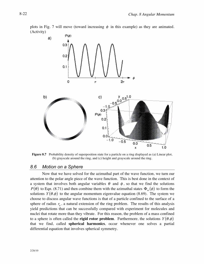
probability density is plotted in Fig. 7 in three different graphical representations. The traditional plot in Fig. 7(a) is similar to the particle-in-a-box plots and conveys the idea of a varying density, but the single dimension fails to make it clear that the left and right ends are connected on the ring and must have the same density. The plot in Fig. 7(b) makes the connection between

! = 0 and

! = 2" clear by plotting the probability density

using color (grayscale) as a parameter along a ring. The plot in Fig. 7(c) combines the ideas of the previous two plots by using both the vertical scale and color to represent the probability density. Because the probability density varies with time also, each of the


2/26/10

8-22

plots in Fig. 7 will move (toward increasing ! in this example) as they are animated. (Activity)

Figure 8.7 Probability density of superposition state for a particle on a ring displayed as (a) Linear plot,

(b) grayscale around the ring, and (c) height and grayscale around the ring.

8.6 Motion on a Sphere Now that we have solved for the azimuthal part of the wave function, we turn our

attention to the polar angle piece of the wave function. This is best done in the context of a system that involves both angular variables ! and ! , so that we find the solutions P !( ) to Eqn. (8.71) and then combine them with the azimuthal states !

m"( ) to form the

solutions Y !,"( ) to the angular momentum eigenvalue equation (8.69). The system we choose to discuss angular wave functions is that of a particle confined to the surface of a sphere of radius

r

0, a natural extension of the ring problem. The results of this analysis

yield predictions that can be successfully compared with experiment for molecules and nuclei that rotate more than they vibrate. For this reason, the problem of a mass confined to a sphere is often called the rigid rotor problem. Furthermore, the solutions Y !,"( ) that we find, called spherical harmonics, occur whenever one solves a partial differential equation that involves spherical symmetry.


2/26/10

8-23

Consider a partcile of mass µ confined to move on a sphere of constant radius r

0.

The wave function ! is independent of r , so derivatives with respect to r are zero and the energy eigenvalue equation (Eqn. (8.38) ) reduces to

!!

2

2µr0

2

1

sin"##"

sin"##"

$%&

'()+

1

sin2"#2

#* 2

+

,-

.

/01 +U (r

0)1 = E1 (8.104)

Following our previous notation, we call the wave function Y ! ,"( ) = P !( )# "( ) . For

this simplified sphere problem, we choose the potential energy U (r

0) to be zero, as in the

ring problem. We identify µr

0

2= I as the moment of inertia of a classical particle of

mass µ moving on a sphere. With these changes, the energy eigenvalue equation is

!!

2

2I

1

sin"##"

sin"##"

$%&

'()+

1

sin2"

#2

#* 2

+

,-

.

/0Y " ,*( ) = EY " ,*( ) (8.105)

As we saw in Eqn. (8.60), we can identify the angular differential operator as the position representation of the angular momentum operator L2 and write the energy eigenvalue equation operator form:

L2

2IY ! ,"( ) = EY ! ,"( ) (8.106)

This looks very similar to the ring problem, but now the angular momentum is not confined to the z-direction because the particle can move anywhere on the sphere. Equation (8.106) is the same eigenvalue equation we found in Eqn. (8.69) for the angular function

Y ! ,"( ) = P !( )# "( ) as long as we identify the separation constant A as

A =2I

!2

E (8.107)

As noted above, we expect that the separation constant A is equal to ! ! +1( ) because

those are the eigenvalues of the L2 operator. Now that we know that this sphere problem is equivalent to the angular momentum eigenvalue equation, we can proceed to solve for the polar angle function P !( ) that we identified in the differential equation (8.71).

8.6.1 Change of Variables The solutions to the ! equation (8.72) that we found in the ring problem told us

the possible values of the separation constant B = m2 , where m is an integer. We now

substitute these known values into the polar angle differential equation (8.71). The ! equation becomes an eigenvalue equation for the unknown unknown function P(!) and the separation constant A :

sin!d

d!sin!

d

d!"#$

%&'+ Asin2! ( m

2"

#$%

&'P(!) = 0 (8.108)

To solve this differential equation, we start with a change of independent variable z = cos! where z is the rectangular coordinate for the particle, assuming a unit sphere.


2/26/10

8-24

As ! ranges from 0 to ! , z ranges from 1 to !1. Using the chain rule for derivatives and sin! = 1" z

2 , the differential term becomes

d

d!=

dz

d!

d

dz= " sin!

d

dz= " 1" z

2 d

dz (8.109)

Notice, particularly, the last equality: we are trying to change variables from ! to z , so it is important to make sure we change all the ! 's to z 's. Multiplying by sin! , we obtain:

sin!d

d!= " 1" z

2( )d

dz (8.110)

Be careful finding the second derivative; it involves a product rule:

sin!d

d!sin!

d

d!"#$

%&'= 1( z

2( )d

dz1( z

2( )d

dz

"#$

%&'

= 1( z2( )

2 d2

dz2( 2z 1( z

2( )d

dz

(8.111)

Inserting Eqn. (8.111) into Eqn. (8.108) and dividing by 1! z2( ) , we obtain a standard form of the associated Legendre's equation:

1! z2( )

d2

dz2! 2z

d

dz+ A!

m2

(1! z2 )

"

#$%

&'P(z) = 0 (8.112)

Once we solve this equation for the eigenfunctions P(z) , we substitute z = cos! everywhere to find the eigenfunctions P(!) of the original equation (8.108).

8.6.2 Series Solution of Legendre's Equation The simplest possible ! dependence is !(") =constant , which corresponds to

the m = 0 eigenstate. Setting m = 0 in equation (8.112) gives us the special case known as Legendre's equation:

1! z2( )

d2

dz2! 2z

d

dz+ A

"

#$%

&'P(z) = 0 (8.113)

This equation is sometimes expressed as

d2

dz2!

2z

1! z2( )

d

dz+

A

1! z2( )

"

#$$

%

&''

P(z) = 0 (8.114)

which emphasizes the mathematical singularities at z = ±1. Let's use the series methods to find a solution of Legendre's equation, i.e. let's

assume that the solution can be written as a series

P(z) =n=0

!

"anz

n (8.115)


2/26/10

8-25

and solve for the coefficients a

n. The differentials

dP

dz=

n=0

!

"annz

n#1 (8.116)

d2P

dz2

=n=0

!

"ann(n #1)z

n#2 (8.117)

substituted into Eqn. (8.113) yield

0 =

n=0

!

"ann(n #1)z

n#2# z

2

n=0

!

"ann(n #1)z

n#2# 2z

n=0

!

"annz

n#1+ A

n=0

!

"anz

n

=

n=0

!

"ann(n #1)z

n#2#

n=0

!

"ann(n #1)z

n# 2

n=0

!

"annz

n+ A

n=0

!

"anz

n

(8.118)

To combine the sums, we need to collect terms of the same powers. To do this, we note that the first two terms in the first sum are zero:

a

0(0)(!1)z

!2+ a

1(1)(0)z

!1= 0 + 0 (8.119)

so we shift the dummy variable n! n + 2 in the first sum, giving

n=0

!

"ann(n #1)z

n#2=

n=#2

!

"an+2

(n + 2)(n +1)zn

=

n=0

!

"an+2

(n + 2)(n +1)zn

(8.120)

Grouping the sums together gives

n=0

!

" an+2

(n + 2)(n +1) # ann(n #1) # 2a

nn + Aa

n$% &' z

n = 0 (8.121)

Now comes the MAGIC part. Because Eqn. (8.121) is true for all values of z , the coefficient of zn for each term in the sum must separately be zero:

a

n+2(n + 2)(n +1) ! a

nn(n !1) ! 2a

nn + Aa

n= 0 (8.122)

Therefore we can solve for the recurrence relation giving a

n+2 in terms of

a

n:

an+2

=n(n +1) ! A

(n + 2)(n +1)a

n (8.123)

Plugging successive even values of n into the recurrence relation Eqn. (8.123) allows us to find

a

2,

a

4, etc. in terms of the arbitrary constant

a

0 and successive odd values of n

allow us to find a

3,

a

5, etc. in terms of the arbitrary constant

a

1. Thus, for the second

order differential equation (8.113) we obtain two solutions as expected. The coefficient

a

0 becomes the normalization constant for a solution with only even powers of z and

a

1


2/26/10

8-26

becomes the normalization constant for a solution with only odd powers of z . For example, the even coefficients are

a2= !

A

2a

0

a4=

6 ! A

12a

2= !

6 ! A

12

"#$

%&'

A

2

"#$

%&'

a0

(8.124)

and the odd coefficients are

a3=

2 ! A

6a

1

a5=

12 ! A

20a

2=

12 ! A

20

"#$

%&'

6 ! A

12

"#$

%&'

a0

(8.125)

so that

P(z) = a0

z0 !

A

2

"#$

%&'

z2+…

(

)*

+

,- + a

1z

1+

2 ! A

6

"#$

%&'

z3+…

(

)*

+

,- (8.126)

We seek solutions that are normalizable, so we must address the convergence of the series solution. Note that for large n, the recurrence relation gives

an+2

an

! 1 , (8.127)

which implies that the series solution we have assumed does not converge at the end points where z = ±1. This is to be expected because the coefficients of Eqn. (8.114) are singular at z = ±1, which correspond to the north and south poles ! = 0," . But there is nothing special about the physics at these points, only the choice of coordinates is special there. This is an important example of a problem where the choice of coordinates for a partial differential equation ends up imposing boundary conditions on the ordinary differential equation which comes from it. To ensure convergence, we thus require that the series not be infinite, but rather that it terminate at some finite power n

max. Inspection

of the recurrence relation in Eqn. (8.123) tells us that the series terminates if we choose

A = nmax

nmax

+1( ) (8.128)

where nmax

is a non-negative integer . When we started this problem, we expected the separation constant to be

A = !(! +1) and now we have found just that, as long as we identify the termination index n

max with the orbtial angular momentum quantum number

! . We have succeeded in finding the quantization condition for orbital angular momentum and it is just as we expected from our work with spin angular momentum. The solutions for these special values of A are polynomials of degree ! , denoted

P!, and

are called Legendre polynomials. The Legendre polynomials can be calculated using Rodrigues' formula:


2/26/10

8-27

P!(z) =

1

2! !!

d!

dz!

z2!1( )

!

(8.129)

The first few Legendre polynomials are:

P0(z) = 1

P1(z) = z

P2(z) =

1

2(3z

2!1)

P3(z) =

1

2(5z

3! 3z)

P4(z) =

1

8(35z

4! 30z

2+ 3)

P5(z) =

1

8(63z

5! 70z

3+15z)

(8.130)

and are plotted in Fig. 8. There are several useful patterns to the Legendre polynomials: • The overall coefficient for each solution is conventionally chosen so that

P!(1) = 1 . As discussed in the next section, this is an inconvenient convention that we are

stuck with! • P!(z) is a polynomial of degree ! .

• Each P!(z) contains only odd or only even powers of z , depending on whether

! is even or odd. Therefore, each P!(z) is either an even or an odd function.

• Because the differential operator in Eqn. (8.113) is Hermitian, we are guaranteed that the Legendre polynomials are orthogonal for different values of ! (just as with Fourier series), i.e.

!1

1

"Pk

*(z)P!(z)dz =

#k!

! +1

2

(8.131)

Note that the Legendre polynomials are normalized; the "squared norm" of P! is

1 / (! + 12 ) .

Figure 8.8 Legendre polynomials.


2/26/10

8-28

Notice that when we substitue the separation constant A back into the original differential equation (8.114)

d2P

dz2!

2z

1! z2

dP

dz+!(! +1)

1! z2

P = 0 , (8.132)

the result is a different equation for different values of ! . For a given value of ! , you should expect two solutions of Eqn. (8.132), but we have only given one. The "other" solution for each value of ! is not regular (i.e. it blows up) at z = ±1. In cases where the separation constant A does not have the special value l(l +1) for non-negative integer values of ! , it turns out that both solutions blow up. We discard these irregular solutions as unphysical for the problem we are solving.

8.6.3 Associated Legendre Functions We now return to Eqn. (8.112) to consider the cases with m ! 0 . We can solve

these equations with a slightly more sophisticated version of the series techniques from the m = 0 case. We again find solutions that are regular at z = ±1 whenever we choose A = !(! +1) for

!! 0,1,2,3,…{ } . With this value for A , we obtain the standard form of

Legendre's associated equation, namely

d2

dz2!

2z

1! z2

d

dz+!(! +1)

1! z2

!m

2

(1! z2 )2

"

#$%

&'P(z) = 0 (8.133)

Solutions of this equation that are regular at z = ±1 are called associated Legendre functions, and are calculated from the Legendre functions:

P!

m(z) = P!

!m(z) = (1! z2 )m/2 d

m

dzm

P!(z)( ) (8.134)

= (1! z

2 )m/2 dm+!

dzm+!

(z2!1)!( ) (8.135)

where m ! 0 . Note that if z = cos! , then P!(z) is a polynomial in cos! , while

(1! z2 )m/2 = (sin2

")m/2 = sinm" (8.136)

so that P!

m(z) is a polynomial in cos! times a factor of sinm! . Some of the associated

Legendre functions are:

P0

0= 1

P1

0= cos!

P1

1= sin!

P2

0=

1

2(3cos2

! "1)

P2

1= 3sin! cos!

P2

2= 3sin2

!

P3

0=

1

2(5cos3

! " 3cos!)

P3

1=

3

2sin!(5cos2

! "1)

P3

2= 15sin2

! cos!

P3

3= 15sin3

!

(8.137)


2/26/10

8-29

and are plotted in Fig. 9. The plots in Fig. 9 are polar plots where the "radius" r at each angle ! is the absolute value of the function P

l

m!( ) , as illustrated in Fig. 10.

Some properties of the associated Legendre functions are

• P!

m(z) = 0 if | m |> !

• P!

!m(z) = P!

m(z)

• P!

m(±1) = 0 for m ! 0 (cf. factor of (1! z2 )m/2 )

Figure 8.9 Polar plots of associated Legendre polynomials.

Figure 8.10 Polar plot of associated Legendre polynomial.


2/26/10

8-30

• P!

m(!z) = (!1)!!mP!

m(z) (behavior under parity)

• !1

1

"P!

m(z)Pq

m(z)dz =2

(2! +1)

(! + m)!

(! ! m)!#!q

The last property shows that for each given value of m , the associated Legendre functions form an orthonormal basis on the interval !1" z "1. Any function on this interval can be expanded in terms of any one of these bases.

8.6.4 Energy Eigenvalues of Rigid Rotor We have now determined the separation constant A in Eqn. (8.108), which

determines the energy of the particle bound to the sphere through Eqn. (8.107). Substituting

A = !(! +1) into Eqn. (8.107) gives the allowed energy eigenvalues

E!="2

2I! ! +1( ) (8.138)

The spectrum of energy levels is shown in Fig. 11. The selection rule for transitions between these levels is !! = ±1 in most cases, yielding the emission lines in Fig. 11. The transition energies are

!E = E!+1

" E!

="2

2I! +1( ) ! + 2( )"

"2

2I! ! +1( )

="2

2I2 ! +1( )

="2

2I2,4,6,8,10,…{ }

(8.139)

A physical example of this particle-on-a-sphere model is the rigid rotor. Consider two atoms with a separation r0 bound to form a molecule, as illustrated in Fig. 12. The moment of inertia of this diatomic molecule about the center of mass is I = µr

0

2 , just as we have assumed in our particle-on-a-sphere model. Molecular spectroscopists define the fundamental rotational constant of the molecule as

B =!2

2I=!2

2µr0

2 (8.140)

and write the energy levels as

E!= B! ! +1( ) (8.141)

As an example, consider the diatomic molecule hydrogen chloride HCl. The equilibrium bond length is r

0= 0.127!nm , which gives a rotational constant

B = 1.32!meV = 10.7cm!1 (8.142)


2/26/10

8-31

Figure 8.11 Energy spectrum and transitions in rigid rotor.

These levels are observed experimentally in rotations of molecules. Experiments on HCl give 2B = 20.8cm

!1 .

8.6.5 Spherical Harmonics Now that we have found the eigenfunctions of the two angular equations, we can

construct the energy eigenstates of the particle on the sphere. The normalized solutions of the ! equation Eqn. (8.72) that satisfy periodic boundary conditions are

!(") =1

2#e

im" (m = 0,±1,±2,...) (8.143)

Figure 8.12 Rigid rotor.


2/26/10

8-32

The normalized solutions of the the ! equation in Eqn. (8.71) that are regular at the poles are given by

P(cos!) =(2! +1)

2

(!" | m |)!

(!+ | m |)! P!

m(cos!) (8.144)

Combining these yields via multiplication (we assumed solutions of this type when we first did the separation of variables procedure), we obtain the spherical harmonics

Y!

m(! ,") = (#1)(m+|m|)/2 (2! +1)

4$

(!# | m |)!

(!+ | m |)!P!

m(cos!)eim" (8.145)

where the somewhat peculiar choice of phase is conventional. The spherical harmonics are orthonormal on the unit sphere:

0

2!

"0

!

" Y!1

m1 # ,$( )( )

*

Y!2

m2 # ,$( )sin#d#d$ = %

!1!2

%m

1m

2

(8.146)

They are complete in the sense that any sufficiently smooth function ! " ,#( ) on the unit

sphere can be expanded in a Laplace series as

! (" ,#) =!=0

$

%m=&!

!

% c!m

Y!

m(" ,#) (8.147)

where

c!m

= !m ! =0

2"

#0

"

# Y!

m $ ,%( )( )*

! ($ ,%)sin$d$d% (8.148)


2/26/10

8-33

Table of spherical harmonics:

! m Y!

m !,"( )

0 0 Y0

0= 1

4#

1 0 Y1

0= 3

4# cos!

±1 Y1

±1= " 3

8# sin!e± i"

2 0 Y2

0= 5

16# 3cos2! $1( )

±1 Y2

±1= " 15

8# sin! cos!e± i"

±2 Y2

±2= 15

32# sin2!e± i2"

3 0 Y3

0= 7

16# 5cos3! $ 3cos!( )

±1 Y3

±1= " 21

64# sin! 5cos2! $1( )e± i"

±2 Y3

±2= 105

32# sin2! cos!e± i2"

±3 Y3

±3= 35

64# sin3!e± i3"

(8.149)

Example 8.2

Given the angular wave function

! (" ,#) =sin" 0 <" <

$2

0 otherwise

%

&'

('

(8.150)

find its representation in terms of spherical harmonics. The representation of the wave function has the form of Eqn. (8.147) and the

expansion coefficients c!m

are determined by Eqn. (8.148):

c!m=

0

2!

"0

! /2

" Y!

m # ,$( )( )*

sin2#d#d$

= N!m

0

2!

"e% im$

d$0

! /2

" P!

m(cos#)sin2#d#

(8.151)

where N!m

is the spherical harmonic normalization constant

N!m

= (!1)(m+|m|)/2 (2! +1)

4"

(!! | m |)!

(!+ | m |)! (8.152)

The azimuthal integral in Eqn. (8.151) is zero unless m = 0 , so


2/26/10

8-34

c!m

=

0 (m ! 0)

(2! +1)"0

" /2

# P!(cos$)sin2$d$ (m = 0)

%

&''

(''

(8.153)

The integral is most easily computed with the substitution z = cos! ; the first few coefficients are:

a00

=!

8a

10=

1

2a

20= "

5!

64

a30

= !7

12a

40= !

9"

512a

50=

77

240 (8.154)

(each of which should be multiplied by

4! / (2! +1) ). As you can check by graphing, however, it requires at least twice this many terms to obtain a good approximation.

8.6.6 Visualization of Spherical Harmonics Visualization of spherical harmonics is a challenge because of the complex nature

and the two-dimensional structure of the wave functions. To overcome the complex problem it is common to plot the complex square, which is the probability density, or to plot the absolute value. In either case, the azimuthal dependence vanishes as we saw with the ring problem earlier. A two-dimensional polar plot, like we used for the Legendre polynomials is therefore sufficent to display the polar angle dependence, as shown in Fig. 13(a). To convey the uniform azimuthal dependence, one should visualize the polar plot as rotated around the vertical z-axis, as displayed in the three-dimensional plot in Fig. 13(b). In the ring case, we also displayed the probability density as a grayscale on the ring itself, which suggests plotting the spherical harmonic probability density as grayscale (or color) on the sphere, as shown in Fig. 13(c). The grayscale sphere can then also be projected onto a flat surface, as mapmakers do, yielding the two-dimensional representation in Fig. 13(d). Note that these plots do not yet give the three-dimensional electron probability density because we still have to learn about the radial wave function in the next chapter.

Figure 8.13 Spherical harmonic Y2

0 !,"( )2

displayed as (a) two-dimensional polar plot, (b) three-dimensional polar plot, (c) grayscale on a sphere, and (d) grayscale on a flat Mollweide projection.


2/26/10

8-35

The polar plots for the first four sets of spherical harmonics are shown in Fig. 14. The standard convention is to label the spherical harmonics, or orbitals, with a letter corresponding to the value of the orbital angular momentum quantum number ! :

! = 0 1 2 3 4 5 6 7 "

letter = s p d f g h i k " (8.155)

The plots in Fig. 14 show angular momentum eigenstate wave functions. In many cases, such as the carbon atom in Fig. 3, the actual orbitals are superpositions, or hybrids, of the angular momentum eigenstates.

Figure 8.14 Polar plots of spherical harmonics.

8.7 Appendix C: Separation of variables The "separation of variables" procedure permits us to simplify a partial

differential equation by separating out the dependence on the different independent varaibles and creating multiple ordinary differential equations. To illustrate the method, we apply a 6-step process to the Schrödinger equation to show how the time dependence of the wave function can be found through an ordinary differential equation in the time variable.

Step 1: Write the partial differential equation in appropriate coordinate system. For Schrödinger's equation in any potential we have:


2/26/10

8-36

H! = i!"!

"t (8.156)

Step 2: Assume that the solution ! can be written as the product of functions, at least one of which depends on only one variable, in this case t . The other function(s) must not depend at all on this variable, i.e. assume

!(r," ,#,t) =$ (r," ,#)T (t) (8.157)

Plug this assumed solution into the partial differential equation Eqn. (8.156). Because of the special form for ! , the partial derivatives each act on only one of the factors in ! .

H!( )T = i!!dT

dt (8.158)

Any partial derivatives that act only on a function of a single variable may be rewritten as total derivatives.

Step 3: Divide by ! in the form of Eqn. (8.157).

1

!H!( )

function of space only

!"# $#

= i%dT

dt

1

Tfunction of time only

!"# $# (8.159)

Step 4: Isolate all of the dependence on one coordinate on one side of the equation. Do as much algebra as you need to do to achieve this. In our example, notice that in Eqn. (8.159), all of the t dependence is on the right-hand side of the equation while all of the dependence on the spatial variable is on the other side. In this case, the t dependence is already isolated, without any algebra on our part.

Step 5: Now imagine changing the isolated variable t by a small amount. In principle, the right-hand side of Eqn. (8.159) could change, but nothing on the left-hand side would. Therefore, if the equation is to be true for all values of t , the particular combination of t dependence on the right-hand side must be constant. By convention, we call this constant E .

1

!H!( ) = i!

dT

dt

1

T" E (8.160)

In this way we have broken our original partial differential equation up into a pair of equations, one of which is an ordinary differential equation involving only t , the other is a partial differential equation involving only the three spatial variables.

1

!H! = E (8.161)

i!dT

dt

1

T= E (8.162)


2/26/10

8-37

The separation constant E appears in both equations. Step 6: Write each equation in standard form by multiplying each equation by its

unknown function to clear it from the denominator.

H! = E! (8.163)

dT

dt= !

i

!ET (8.164)

Notice that Eqn. (8.163) is an eigenvalue equation for the Hamiltonian operator H . That's just the energy eigenvalue equation that we know and love. It is often also called the "time independent Schrödinger equation" because of the way we obtained it here with the the separation of variables procedure. Equation (8.164) is the equation for the time dependence of quantum state vectors that we solved in Chap. 3.

8.8 Problems

1) Show that the two-body Hamiltonian can be separated into center-of-mass motion and relative motion, as in Eqn. (8.11). Do this in two ways: (a) with momentum operators in the abstract, and (b) momentum operators in the position representation.

2) Use the separation of variables procedure to justify the assertion leading to Eqn. (8.24).

3) Use the separation of variables procedure in Appendix C to break equation Eqn. (8.29) up into three ordinary differential equations.

4) Using Eqns.. (8.35) and (8.41), show that the orbital angular momentum operators Lx, Ly , and L

z are represented in spherical coordinate as

Lx! i" sin!

""#

+ cos! cot#""!

$%&

'()

Ly! i" * cos!

""#

+ sin! cot#""!

$%&

'()

Lz! *i"

""!

and verify that the operator L

2= LiL= L

x

2+ L

y

2+ L

z

2 is represented in spherical coordinate as in Eqn. (8.60)

5) Use the separation of variables procedure on the angular Eqn. (8.69) to obtain Eqn. (8.71) and Eqn. (8.72) for the polar and azimuthal angles.

angular momentum & ring/sphere - physics at oregon state

Documents