Angular Radial Edge Histogram

Columbia University, ADVENT Technical Report #218-2006-4, November 5, 2006

Barry Rafkind and Shih-Fu Chang Abstract The Angular Radial Edge Histogram (AREH) extends prior work on a compact image representation based on geometric distributions of edge pixels. Histograms of edge pixels are computed along the dimensions of angle and radius. Fourier transform is applied to accommodate rotation invariance. It achieves invariance for scale variation, in-plane rotation, and translation. By using a grid-based approach, it can also handle limited cases of partial occlusions. Our method is efficient � it does not require image segmentation or edge linking. We have evaluated its performance using an extensive set of test data including 12 different types of variations over diverse images (schematic diagrams and photos). Experimental results in image retrieval show that AREH outperforms baseline solutions using global edge direction histograms by a large margin. 1. Introduction Accurate real-world content-based image retrieval requires search techniques that are robust to a range of distortions. One way to achieve this is to use image features that are invariant to geometric distortions such as scaling, rotation, and translation in addition to other types of distortions that introduce noise, for instance. Edge-based methods attempt to extract the edges that correspond to objects and textures in the image. Such approaches are consistent with the observation that objects and textures are considered salient for image retrieval and that they are well defined by their characteristic edge information. Edges and textures are especially useful for representing and matching schematic images. See Figure 1.

Figure 1 : Examples of Schematic Images

Section 2 provides a review of the state of the art in content-based image retrieval. Section 3 describes prior work on a highly related approach proposed by Chalechale et al. called Angular Radial Partitioning (ARP) [1]. Section 3 and its subsections explain the details of our approach. Section 4 discusses differences between our approach and the ARP. Section 5 contains our experiments and results. Conclusions and Future Work are found in Section 6 followed by References. 2. Review of the State of the Art In their 1998 survey, Rui, Huang, and Chang summarized the advancements in CBIR and proposed open issues based on the state of the art methods [2]. The image feature representations discussed include color histogram, color moments, color sets, color layout, texture properties, wavelet representations, region-based, and boundary-based descriptors.

More recently, Mahmoudi et al. proposed a shape-based approach for image indexing and retrieval called Edge Orientation AutoCorrelogram (EOAC) [3]. The EOAC represents an image by a 2-dimensional histogram. One dimension depends upon the orientation of edges. The other dimension controls the distance neighborhood of edges in the same orientation. The authors showed the superiority of this technique over edge direction histogram.

A popular research trend over the last few years is known as parts-based CBIR (also related to Multiple Instance Learning [4]). Techniques in this category represent images as a collection of parts (such as interest points or regions) and possibly part relations (such as inter-part distances, angles, or a description of the connecting path). Following part-detection, the image region associated with each part may or may not be normalized to achieve certain invariance properties. Feature descriptors are then computed for each part and part relation. Parts-based representations may provide greater robustness to structural distortions such as warping or occlusion by preserving salient local structures while decoupling them from their spatial relationships. This contrasts with the ARP and AREH approaches which rely on maintaining spatial structure.

The different parts-based methods are uniquely characterized by the subsequent steps for processing sets of features and calculating the similarity between them. Dongqing Zhang introduced the Attributed Random Graph method that can be used for image retrieval and near duplicate image detection [10]. Sivic and Zisserman developed an efficient image indexing approach for searching through video called Video Google [5]. Grauman and Darrell invented the Pyramid Match Kernel for image classification [6].

For the Attributed Random Graph (ARG), image similarity derives from a probability ratio that depends on the distribution of features learned across pairs of labeled positive (duplicate) and negative (non-duplicate) images as well as the likelihood of transformation between sets of features from images pairs. By learning the distribution of part-based features from the image set, this method can adapt to any specific domain even if it grows or changes over time. Another important aspect of this technique is that it explicitly models part-relations by incorporating them into the probabilistic transformation, rather than treating proxomity constraints in a separate step.

Video Google aims at allowing the user to crop any object or region in a frame of video and quickly return the other frames containing it. The authors accomplish this by reducing the CBIR challenge to the standard text-retrieval paradigm. First, image features are vector quantized according to a visual vocabulary defined by a set of global prototypes obtained by clustering the sets of features from a training pool of images. In this way, each image can be represented by a weighted frequency vector just as text documents are indexed by search engines such as Google. An inverted file accelerates the process by focusing the search only on candidate images which share visual terms with the query.

The Pyramid Match Kernel avoids the probabilistic assumptions and complexities in the ARG method as well as the loss in discriminative power inherent in vector quantization approaches such as Video Google. Essentially, the idea is to take the high-dimensional feature space populated by features from two images and split the space by multiple histograms of increasing resolution. The similarity between two feature sets is calculated as the weighted combination of histogram intersections at corresponding resolutions. The authors claim that this technique approximates the optimal correspondences between the features. Advantages include high retrieval efficiency as well as robustness to noise and to variations in the sizes of sets (cardinality).

As mentioned above, all parts-based CBIR methods require part detectors and feature descriptors. Certain invariance properties can not be obtained without choosing robust part detectors and features descriptors. Therefore, another avenue of our research concerns the optimal selection and tuning of these essential components. Popular part detectors include the Harris-Affine interest point detector [7] and the Maximally Stable region detector [8] used in Video Google. One of the most popular feature descriptors is Lowe�s SIFT descriptor [9].

3. Angular Radial Partitioning 3.1 Method Overview The ARP approach consists of three major steps: First, preprocess the image (section 3.2), then partition the edge map into radial and angular sectors to make a histogram (section 3.3), and finally create the rotationally invariant descriptor by taking the 1D Fourier Transform of the histogram (section 3.4). The authors propose using the L1 distance metric (section 3.5). 3.2 Preprocessing � grayscale, edge extraction, resize image There are three defined preprocessing steps: grayscale conversion, edge extraction, and image resizing. These steps are necessary to prepare the image for the histogram calculations in the next section. In step 1, project the color image into HSV color space. Then throw away the hue and saturation and keep the luminance (value) component to obtain a grayscale image. In step 2, perform edge detection on the grayscale image with an edge extraction operator, such as the Canny or Sobel edge operator. In step 3, normalize the edge map to W x W pixels. This resizing step attempts to achieve scale invariance for the image. Finally, threshold the edges to find the significant edges. Represent the edge pixels as 1�s and non-edge pixels as 0�s. 3.3 Histogram Computation Partition the normalized edge map into M radial divisions and N angular divisions. The angle between adjacent angular partitions is θ = 2π/N and the difference in radius between successive concentric circles is ρ = R/M where R is the radius of the circle surrounding the W x W image. Next, count the number of edge pixels in each sector and form a histogram across all sectors: (insert formula here) 3.4 FFT for Rotational Invariance An image rotation corresponds to a shift in the angular dimension of the histogram. Taking the 1-dimensional Fourier Transform of the discrete histogram yields an extra complex exponential due to this shift. We can thus theoretically achieve rotational invariance by taking the absolute value of the FFT across the angular dimension to remove this extra term. However, this only yields true

rotational invariance if the rotation is a multiple of 2π/N. Otherwise the rotated pixels will be divide between adjacent partitions, and the histogram will distort such that the absolute FFT will no longer compensate for this rotation. The absolute 1D FFT is computed in the angular dimension, thus the resulting feature is still 2-dimensional. 3.5 Distance Metric The L1 �Manhattan� distance is taken between two images. It is the sum of the absolute differences between corresponding terms in the 2-dimensional ARP feature. (insert L1 formula here). 4. Angular Radial Edge Histogram 4.1 Method Overview The Angular Radial Edge Histogram (AREH) was developed independently and without knowledge of the ARP method. There are just a few key differences between them as presented below. 4.2 Preprocessing Steps � grayscale, edge extraction Similar to the ARP preprocessing steps, the AREH requires conversion of the image to grayscale and edge extraction. However, image rescaling is not performed. 4.3 Histogram Computation In contrast to the ARP method, the AREH does not fit a circle around the image for radial standardization. Instead, the center of mass (centroid) of the edge pixels are found and the maximum radius, R, is chosen as the largest distance between any pixel and the centroid. Due to the different normalization method, our approach achieves invariance to scaled content within the same image size.To state this in another way, we expect to compute similar features for two images in which one has a scaled version of the content of the other while the sizes of both images are equal or different. Apart from this difference, the histogram computation is the same as in the ARP. We divide the image into M x N partitions and count the number of pixels in each sector.

4.4 FFT for Rotational Invariance As in the ARP method, we take the absolute value of the 1D FFT along the angular dimension of the 2D histogram to achieve rotational invariance. The motivation for doing this is the same as in the ARP. By truncating the FFT, the feature descriptor size may be reduced without sacrificing much retrieval accuracy. 4.5 Grid Features for Partial Images The partial image distortion represents a particularly challenging obstacle to the ARP method. In this image variation, some of the content has been replaced by a uniform color so that an area of the edge map disappears. This may shift the centroid of the edge pixels to a different location and change the global histogram significantly.

Figure 2 : Flow Diagram shows Original Schematic on Left, Binary Edge Map in Center, and Grid Partitions on Right

To counter this effect, we divide the edge map up into a grid of Q x P rectangular regions. Then for each grid region, calculate the AREH feature based on the center point of the region (not the centroid). These grid features are obtained in addition to the global feature that uses the centroid for distance calculations. Thus, we have 1 + QxP AREH features for each image. The grid approach is based on the assumption that only those grid regions affected by the distortion will change while the remaining regions will remain unchanged. The obvious drawback to this technique is that it also assumes no simultaneous geometric variations such as translation, rotation, or scaling in addition to the partial image distortion. If a combination of distortions were to occur simultaneously, then the global feature and all grid features could change dramatically yielding very little invariance. An alternative method to combat the partial image distortion would be to take the normal global feature that uses the edge centroid in addition to another

global feature that uses the image center point. Fixing the reference point at the center on the global scale should yield a feature that is equally invariant to the partial distortion, yet would similarly be sensitive to concurrent distortions such as translation. Thus, we would obtain two global features in this way, rather than the 1+QxP features obtained using the grid approach. Although this would be simpler and less computationally intensive than the grid approach, the author did not have time to evaluate this alternative. 4.6 Similarity Metric Two issues are apparent upon considering the choice of similarity metric between AREH features. First, we note strong reasons why the L1 distance is not optimal for comparing features, although the inventors of the ARP approach used this. Second, a balance must be found in weighting the relative importance of the similarity among the grid features versus the global features. The authors of the ARP method suggest using the L1 distance between features, but without any justification. However, there are some situations in which the L1 distance would not be optimal. Consider two images where one has the same edge shape as the other, but just contains fewer edge pixels in each bin of the histogram. The L1 distance would be large between the features, even though they are very similar. Thus, a more appropriate distance or similarity metric would look at the correlation of the features, rather than just the difference in magnitude. We suggest using the cosine distance (correlation) between features instead of the L1 distance metric. Two features, A and B, can be represented as matrices with elements indexed by the variables i and j. Then the formula (1.1) gives the correlation :

( )( )( ) ( )

Cosine Distance ij ij ij ij

ij

ij ij ij ijij ij

a a b b

a a b b

− −=

− −

∑

∑ ∑ (1.1)

The value of the cosine distance extends from a minimum of �1 for signals with an angle of pi between them to a maximum of +1 for signals with angles of zero or 2pi. The cosine distance metric compares the angle between two signals rather than the difference in magnitude which is what the L1 distance measures. This property of the cosine distance metric helps make it invariant against relative in-plane scaling of the image content.

The AREH yields a set of features for each image: the global feature and the grid features. The global feature will help match images that do not suffer from the partial image distortion while the grid features will. We could perhaps give a relative weighting to the importance of the grid features if we knew a priori what proportion of images in our dataset had the partial variation. Lacking this knowledge, we consider the two types of features equally important and thus we need a corresponding way to combine them. As mentioned previously, the correlation between two global features will have a maximum value of 1 if a perfect match is found. Thus, we also want the grid feature similarity to have a maximum value of 1 so that it can be equally weighted with the global features. An obvious way to accomplish the goal of normalizing the grid similarity is to take an average over all the similarities between corresponding grid features. However, this unfortunately gives very low similarities among the grid features for a partial image compared with the original. If half of the grid features are zero due to partial distortion, then the largest averaged grid similarity would be ½. Doing this would make the partial image similarity much weaker against the global features in a situation where it is actually the more important part. Thus, we do not want to average over all the grid features, but just those for which the query has non-zero grid features.

Figure 3 : Representation of similarity calculations from Global and Grid features. Left column shows features for the Query image. Middle column shows features for the Target image. Right column shows the cosine distance values between corresponding features.

( )Similarity = 0.4 0.0 0.2 0.0 0.3 0.4 - 0.1 0.1 7 0.53+ + + + + + = (1.2)

Figure 3 represents the similarity calculations for the global and grid features. Since the query features have 7 non-zero grid features, only the corresponding set of similarity values is averaged, not all 9. The final similarity results from the sum of the global and averaged grid similarity values. In summary, our similarity procedure finds the correlations between all corresponding pairs of features at the global and grid level. The set of grid correlations is then averaged by the number of non-zero query grid features and then this average is added to the global correlation to produce an overall similarity metric that will be close to 0 for dissimilar images and close to 2 for perfectly identical images. 5. Notable Differences between ARP and AREH The AREH contains several techniques that do not exist in the ARP. They are the inclusion of a noise removal step, a modified radial partitioning method, a grid approach, and a different similarity metric. The noise removal step makes the AREH more robust to noise than the ARP. Using the centroid for the global feature rather than the image center makes the AREH translation invariant. Normalizing the distances by the maximum edge distance makes the AREH invariant to scaled content in a static image size while the ARP is only invariant to whole image scaling. For the AREH, the grid approach achieves invariance to the partial image distortion in the absence of other distortions. Finally, using the correlation instead of the L1 distance metric should make the AREH better at finding similar images when the edge shapes are similar despite differences in the number of edge pixels. 6. Experiments 6.1 Retrieval Task We tested the performance of the AREH for an image retrieval task. The goal was to use a distorted version of an original as the query into the original dataset and rank the images such that the original match would appear near the top of the results. 6.2 Dataset Our dataset contains 12 sets of 1200 JPEG images size 826x1169 in 24 bit color depth. One of the sets contains the original images while each of the other folders has a different distortion applied to it. The original images are scanned pages from a technical manual and have no colors besides shades of gray.

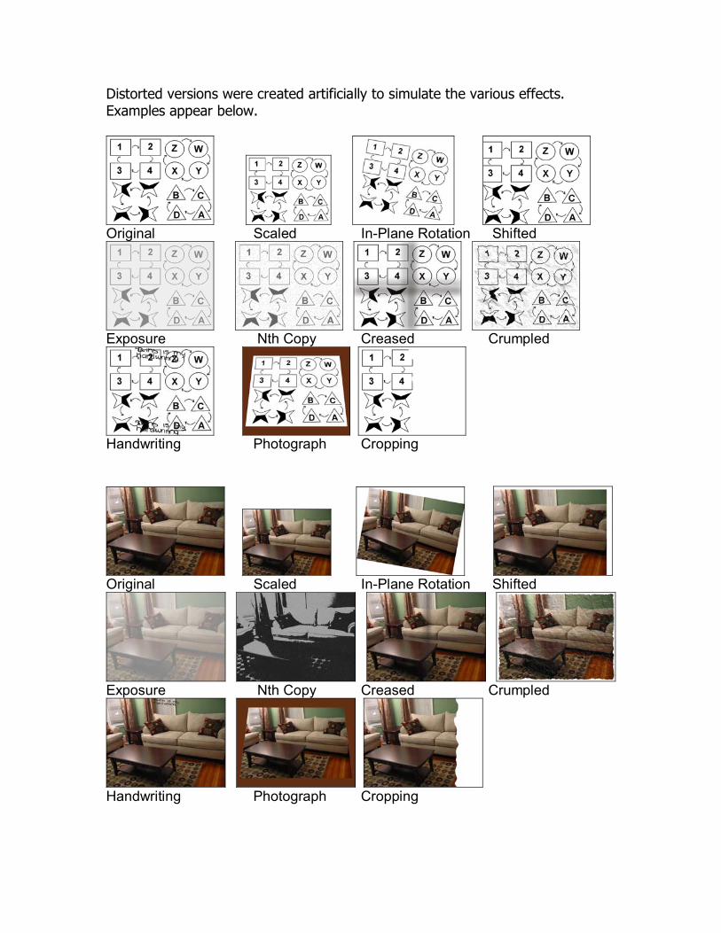
Distorted versions were created artificially to simulate the various effects. Examples appear below.

Original Scaled In-Plane Rotation Shifted

Exposure Nth Copy Creased Crumpled

Handwriting Photograph Cropping

Original Scaled In-Plane Rotation Shifted

Exposure Nth Copy Creased Crumpled

Handwriting Photograph Cropping

6.3 Implementation and Experiments In our implementation of the AREH, the Sobel edge operator was used to detect edges. In the noise removal step, clusters with 20 or fewer pixels were removed. We used 3x3 overlapping regions for the grid computation. Each grid region overlapped with about 2/3 of any neighboring region. We used 100 radial bins and 360 angular bins for each image. We used the 2D FFT instead of the 1D FFT. The 2D FFT showed slight improvement in retrieval performance for a few test cases, so we continued to use it. However, we do not think it is any better than the 1D FFT for gaining rotational invariance. We conducted a series of experiments with the assumption that the lower frequencies of the Fourier spectrum represent the histogram content the best. The experiments tested varying feature dimensionalities by extracting different regions from the 2D FFT of the 100x360 dimension AREH histogram. Our first experiment varied the feature dimensionality but only used between global descriptors for retrieval (results in Table 2). The second experiment varied the feature dimensionality using both the global descriptor and all nine grid descriptors in the fusion scheme described in section 3.6 (results in Table 3). 6.4 Evaluation Metric We assume that the user wants to see the matching image on the first �page� of the ranked result set. Taking a page size to be 21 returned images, we define our evaluation metric as the percentage of all non-empty (contains edge content) queries that return a match in the top 21 results. 6.5 Results The full feature using 10 transforms (25 radial dimensions, 90 angular dimensions) requires about 180 x 103 bytes of disk space per image, regardless of image size or complexity.

The color codes in Table 1 should simplify the visual understanding of our evaluation.

Note that the average matching time per query is not very stable. Although it correlated with the size of the feature, it also highly depended on the CPU load of the server used to run the simulations. Thus, there was some fluctuation, since the servers were shared with other research students.

From the results, it is clear that the AREH descriptor is robust to Affine transformations including scaling, rotation, and translation. It also displays robustness to physical variations including exposure, nth copy, creasing, crumpling, handwriting, and rasterization. We observe that the global descriptor struggles with the partial and photo distortions. As expected, the grid feature improved performance in the partial variation significantly. Performance improvement occurs also for the photo distortion. This can probably be explained by considering the effect of an artificial border introduced by the photo distortions. A border around the edge of an image could significantly affect the location of the edge centroid. However, since the grid features use the centers of the grid areas, an image edge would not have as great of an effect. We note that for many distortions, a drastic reduction in feature dimensionality does not change retrieval performance significantly. Ultimately, the choice of feature size will depend on the retrieval specifications and storage capacity of the user�s system.

Angular Radial Edge Histogram �Page 1� Results

Color Codes Perfect 100%

Near-Perfect

95-100%Good

90-95% Moderate80-90%

Poor 70-80%

Failing under 70%

Table 1 : Page 1 Evaluation Metric Color Codes

Page 1 Evaluation Measurements for Global Descriptor

Radial Dimension 25 15 10 10 5 10 5 4Angular Dimension 90 45 20 10 10 5 5 4Total Dimension Per Transform 2250 675 200 100 50 50 25 161 Scaled 99.75 99.08 98.91 99.00 98.91 98.66 98.50 98.082 Rotated 99.67 99.50 99.42 99.42 99.42 98.91 99.00 99.003 Shifted 99.83 99.50 99.50 99.58 99.83 99.83 99.75 99.584 Exposure 88.80 88.21 88.21 88.13 88.13 87.79 87.88 88.045 Nth Copy 98.50 98.25 98.33 98.25 98.33 98.00 97.92 97.756 Creased 99.92 99.75 99.75 99.75 99.75 99.67 99.67 99.587 Crumpled 89.50 87.75 89.00 88.67 89.75 85.50 85.83 80.008 Partial 31.65 28.35 28.02 28.60 27.43 27.43 27.51 26.259 Handwriting 87.33 83.75 84.17 85.00 86.00 83.00 81.42 75.6710 Photo 68.25 62.67 64.25 64.25 65.42 56.33 55.83 45.4211 Rasterization 96.41 94.31 94.73 95.07 95.65 94.57 94.48 92.81Average Score 87.24 85.56 85.84 85.88 86.24 84.52 84.34 82.02Avg Match Time Per Query (sec) 2.67 2.04 2.63 2.60 1.87 1.86 1.85 1.89

Table 2 : Retrieval Results using only Global descriptor

Page 1 Evaluation Measurements for Global + 3x3 Grid Descriptor

Radial Dimension 25 15 10 10 5 10 5 4Angular Dimension 90 45 20 10 10 5 5 4Total Dimension Per Transform 2250 675 200 100 50 50 25 16

Total Dimension Per Image 22500 6750 2000 1000 500 500 250 1601 Scaled 100.00 100.00 100.00 100.00 100.00 100.00 100.00 99.922 Rotated 95.83 92.98 90.38 87.12 81.77 78.26 71.57 61.373 Shifted 99.83 99.75 99.75 99.75 99.67 99.67 99.50 98.584 Exposure 91.64 91.97 99.75 90.64 90.55 90.55 90.55 90.385 Nth Copy 99.25 99.33 90.56 99.25 99.25 99.25 99.25 99.086 Creased 100.00 100.00 100.00 100.00 100.00 100.00 100.00 100.007 Crumpled 95.17 93.75 94.92 95.42 95.58 95.33 95.33 94.508 Partial 77.55 71.73 63.88 57.05 53.08 53.08 47.76 44.229 Handwriting 97.00 96.58 96.08 96.00 95.92 95.08 94.92 94.5010 Photo 81.42 70.58 71.42 73.92 74.75 73.67 73.83 71.5011 Rasterization 99.75 99.67 99.67 99.58 99.50 99.67 99.58 99.50Average Score 93.51 92.40 91.46 90.79 90.00 89.26 88.39 86.69Avg Match Time Per Query (sec) 22.84 11.15 17.85 17.41 12.58 11.85 16.20 15.53

Table 3 : Retrieval Results using Global + Grid Descriptors

6. Conclusions and Future Work We presented a new image feature that extends the work of the ARP method. The AREH shows good robustness to many types of distortions. Its benefit over the ARP is improved robustness against noise and partial images, scaled content in static image size, and a more intuitive similarity metric. Both the ARP and AREH suffer from requiring the user to tune many design parameters. This might afford these approaches flexibility over a wide range of application areas, but it also means that many users will find these techniques quite demanding to work with. The strength of these image descriptors lies in their ability to retain the relative spatial geometry of the image in a robust and compact form. This contrasts with other image features such as color histograms and moment-based features that lose a sense of spatial structure. In the future, we would like to further investigate the effect of varying the design parameters such as the number of angular and radial partitions. Additionally, we would like to see if comparable retrieval accuracy can be achieved by computing smaller initial AREH histograms before taking the Fourier transform.

In addition, it would be interesting to try a soft binning approach rather than a hard assignment of edge pixels in to the histogram bins. The choice of edge detector and edge threshold can be investigated as well as different noise removal schemes. We might also try to compare the grid approach to a fixed global feature that uses the image center. Finally, it should be noted that this feature does well for the given problem, that of matching a distorted image to its original version. However, neither the ARP nor the AREH would probably do well for finding semantically similar images with quite different edge maps, because these methods are highly sensitive to the edge structure. Acknowledgement We thank Eric Zavesky and Dongqing Zhang for their assistance and discussion. This material is based upon work funded in whole by the U.S. Government. Any opinions, findings and conclusions or recommendations expressed in this material are those of the authors and do not necessarily reflect the views of the U.S. Government. References 1. A. Chalechale, A. Mertins, and G. Naghdy, �Edge image description using angular radial partitioning,� IEE Proc. Vision, Image & Signal Processing, vol. 151, no. 2, pp. 93�102, April 2004.

2. Yong Rui, Thomas S. Huang, and Shih-Fu Chang, "Image retrieval: current

techniques, promising directions and open issues", Journal of Visual

Communication and Image Representation, Vol. 10, no. 4, pp. 39-62, April 1999

3. Mahmoudi, F., Shanbehzadeh, J., Moghadam, A.M.E., Zadeh, H.S., 2003.

Image Retrieval Based on Shape Similarity by Edge Orientation Autocorrelogram.

Pattern Recognition 36, 1725-1736.

4. O. Maron and T. Lozano-Pérez. A framework for Multiple-Instance Learning. In

Advances in Neural Information Processing Systems 10. MIT Press, 1998

5. J. Sivic and A. Zisserman, Video google: A text retrieval approach to object

matching in videos, in Proceedings of the 9th International Conference on

Computer Vision, Nice, France, 2003.

6. Kristen Grauman, Trevor Darrell, "The Pyramid Match Kernel: Discriminative

Classification with Sets of Image Features," iccv, pp. 1458-1465, Tenth IEEE

International Conference on Computer Vision (ICCV'05) Volume 2, 2005.

7. K. Mikolajczyk and C. Schmid. An affine invariant interest point detector. In

Proceedings of the 7th European Conference on Computer Vision, Copenhagen,

Denmark, volume I, pages 128�142, May 2002.

8. J. Matas, O. Chum, M. Urban, and T. Pajdla. Robust wide baseline stereo from

maximally stable extremal regions. In Proceedings of the 13th British Machine

Vision Conference, Cardiff, England, pages 384�393, 2002.

9. D. G. Lowe. Object recognition from local scale-invariant features. In

Proceedings of the 7th International Conference on Computer Vision, Kerkyra,

Greece, pages 1150�1157, 1999.

10. Dong-Qing Zhang and Shih-Fu Chang, "Statistical Part-Based Models: Theory

and Applications in Image Similarity, Object Detection and Region Labeling", PhD

Thesis Graduate School of Arts and Sciences, Columbia University, Chapter 2,

2005.