Animating Bubble Interactions in a Liquid Foam

Oleksiy Busaryev∗

Ohio State UniversityTamal K. Dey∗

Ohio State UniversityHuamin Wang∗

Ohio State UniversityZhong Ren†

Zhejiang University

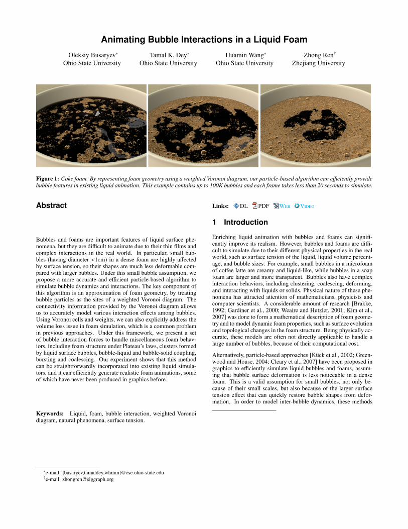
Figure 1: Coke foam. By representing foam geometry using a weighted Voronoi diagram, our particle-based algorithm can efficiently providebubble features in existing liquid animation. This example contains up to 100K bubbles and each frame takes less than 20 seconds to simulate.

Abstract

Bubbles and foams are important features of liquid surface phe-nomena, but they are difficult to animate due to their thin films andcomplex interactions in the real world. In particular, small bub-bles (having diameter <1cm) in a dense foam are highly affectedby surface tension, so their shapes are much less deformable com-pared with larger bubbles. Under this small bubble assumption, wepropose a more accurate and efficient particle-based algorithm tosimulate bubble dynamics and interactions. The key component ofthis algorithm is an approximation of foam geometry, by treatingbubble particles as the sites of a weighted Voronoi diagram. Theconnectivity information provided by the Voronoi diagram allowsus to accurately model various interaction effects among bubbles.Using Voronoi cells and weights, we can also explicitly address thevolume loss issue in foam simulation, which is a common problemin previous approaches. Under this framework, we present a setof bubble interaction forces to handle miscellaneous foam behav-iors, including foam structure under Plateau’s laws, clusters formedby liquid surface bubbles, bubble-liquid and bubble-solid coupling,bursting and coalescing. Our experiment shows that this methodcan be straightforwardly incorporated into existing liquid simula-tors, and it can efficiently generate realistic foam animations, someof which have never been produced in graphics before.

Keywords: Liquid, foam, bubble interaction, weighted Voronoidiagram, natural phenomena, surface tension.

∗e-mail: {busaryev,tamaldey,whmin}@cse.ohio-state.edu†e-mail: zhongren@siggraph.org

Links: DL PDF W V

1 Introduction

Enriching liquid animation with bubbles and foams can signifi-cantly improve its realism. However, bubbles and foams are diffi-cult to simulate due to their different physical properties in the realworld, such as surface tension of the liquid, liquid volume percent-age, and bubble sizes. For example, small bubbles in a microfoamof coffee latte are creamy and liquid-like, while bubbles in a soapfoam are larger and more transparent. Bubbles also have complexinteraction behaviors, including clustering, coalescing, deforming,and interacting with liquids or solids. Physical nature of these phe-nomena has attracted attention of mathematicians, physicists andcomputer scientists. A considerable amount of research [Brakke,1992; Gardiner et al., 2000; Weaire and Hutzler, 2001; Kim et al.,2007] was done to form a mathematical description of foam geome-try and to model dynamic foam properties, such as surface evolutionand topological changes in the foam structure. Being physically ac-curate, these models are often not directly applicable to handle alarge number of bubbles, because of their computational cost.

Alternatively, particle-based approaches [Kuck et al., 2002; Green-wood and House, 2004; Cleary et al., 2007] have been proposed ingraphics to efficiently simulate liquid bubbles and foams, assum-ing that bubble surface deformation is less noticeable in a densefoam. This is a valid assumption for small bubbles, not only be-cause of their small scales, but also because of the larger surfacetension effect that can quickly restore bubble shapes from defor-mation. In order to model inter-bubble dynamics, these methods

typically treat each bubble as a sphere, and then they apply inter-action forces whenever two spheres intersect. While this approachis sufficient for standalone bubbles, it fails to properly capture con-nectivity when bubbles form clusters and is of limited use in mod-eling surface-tension-based interaction among bubbles on a liquidsurface. How to maintain volume conservation for each individualbubble is another challenging problem for these techniques, sincefoam geometry and bubble shapes are not explicitly represented.

To solve these problems, we propose a simple and efficient particle-based algorithm that can simulate realistic bubble interactions incomplex foam scenarios, as shown in Figure 1. The basic idea be-hind this method is to represent bubbles using weighted points andgather them into a weighted Voronoi diagram. Our work shows thatthe algorithm can benefit from using this diagram in three ways.First, it explicitly reveals bubble connectivity. From the weightedVoronoi diagram, we can directly infer which two bubbles share theliquid film, and which bubbles are potential candidates for tension-based interaction. The Voronoi diagram allows us to accuratelymodel the instability of multiple-bubble intersections that is quicklyresolved into triple (in 2D) or quadruple (in 3D) intersections in thereal world. Secondly, it provides a simple and natural approxima-tion to the actual foam geometry, and it can be directly used forrendering. Finally, the weighted Voronoi diagram can be used toexplicitly calculate bubble volumes, which is a crucial componentin the volume correction process.

Our system pipeline starts each time step with formulating bub-ble interaction forces, based on the bubble connectivity informa-tion provided by the weighted Voronoi diagram. The forces arethen used in an implicit integrator to evolve bubble positions andvelocities over time. After that, it calculates the volume of eachbubble using the Voronoi cell, and compensates volume changes byadjusting the Voronoi weight. Finally, the system handles burstingand coalescing effects by performing topological changes, and itreconstructs the weighted Voronoi diagram for the next time step.

In summary, we propose a novel particle-based algorithm to sim-ulate bubble interactions in a liquid foam, by making the follow-ing contributions: 1) a weighted Voronoi representation that modelsbubble connectivity and foam geometry; 2) a set of bubble interac-tion forces that can produce various interaction behaviors; and 3) avolume correction method for particle-based bubbles. We illustrateour method with animations of typical real-world foam scenarios,including clustering, stacking, sticking to liquid or solid surfaces,bursting and coalescing. We also incorporate this method into aparticle level set liquid simulator, and test its capability of addingrealistic bubbles and foams in liquid animation.

2 Previous WorkFoam Physics. Real-world foams exhibit significantly differentstructures and dynamic behaviors due to their physical properties.A dry foam, in which the liquid volume is typically less than 1 per-cent of the whole volume, can form a specific structure under lawsdiscovered by the Belgian physicist Joseph Plateau. Taylor [1976]later proved that this structure minimizes the bubble surface areaunder volume constraints. Different from the dry foam, a wet foamhas more complex structures due to its liquid volume, and it hasbeen studied in multiple ways [Weaire et al., 1993; Herzhafta et al.,2005; Piazza et al., 2008]. Foam structures can also be classified ac-cording to their bubble sizes, such as monodisperse foam [Krayniket al., 2003] that contains uniformly sized bubbles and polydis-perse foam [Kraynik et al., 2004], in which the bubble size canvary. Compared with foam structure, foam dynamics is a less stud-ied problem due to the difficulty in observing dynamic behaviors,including drainage, rheology, coarsening, and merging. A compre-hensive study on both foam structure and foam dynamics can be

found in Weaire and Hutzler’s book [2001]. In this paper, we focuson simulating rheological and merging behaviors of polydispersefoams, in both dry and wet cases for graphics applications.

Due to the similarity between the weighted Voronoi diagram andfoam geometry, physicists studied using the diagram to model staticfoam structures [Redenbach et al., 2012] in the past. Although theyalso used the diagram to initialize foams in dynamic simulation,they chose to solve bubble dynamics using more sophisticated mod-els [Kraynik et al., 2004; Brakke, 1992] instead, since only a smallset of bubbles were considered in their typical examples. In con-trast, we found the weighted Voronoi diagram can be used directlyin dynamic simulation as well, and it provides a good approxima-tion to foam structure for a great number of bubbles.

Foam Simulation. The simulation of bubbles and foams in-volves two aspects: the deformation of individual bubble surfaces,and the interactions among bubbles, liquids and solids. An earlyexample of deformable bubbles is proposed by Brakke [1992].Durikovic [2001] used a spring mesh to represent bubble surfacesand approximated interaction forces using an intermolecular Vander Waals force model. To facilitate topological changes, Kim etal. [2011] developed a 2D algorithm using the immersed bound-ary method. Kelager [2009] introduced the ghost bubble techniqueto the vertex-based dry foam simulation. Implicit representations,such as Volume-of-Fluid (VOF), can also be used to simulate de-formable bubbles, as Hong et al. [2003] and Mihalef et al. [2006]showed. Zheng et al. [2006] proposed a regional level set method toimplicitly model liquid foams as multi-manifold surfaces. Kim etal. [2007] addressed the volume loss in the regional level set methodusing a volume control technique. While these methods can handlesurface deformation of individual bubbles, they need considerablecomputational time to handle a large number of bubbles.

By ignoring surface deformation, particle-based techniques arespecifically developed for handling bubble interactions with the en-vironment. Durian [1995] first proposed to use a mass-spring modelto animate bubble interactions in 2D. Kuck et al. [2002] extendedthis idea to 3D, and also developed a way to render Plateau bor-ders and curved films between contacting bubbles. Greenwood andHouse [2004] incorporated the Kuck model into a particle-level-set-based liquid simulator. Bubble interactions may also be approx-imated by Smoothed Particle Hydrodynamics (SPH) as in [Clearyet al., 2007; Thurey et al., 2007; Hong et al., 2008], though theytypically do not consider internal foam geometry. While we alsorepresent bubbles as particles in our system, we improve simula-tion accuracy by the use of weighted Voronoi diagrams, and we canhandle more bubble interaction behaviors.

Fluid Simulation. Fluid simulation is an important researchtopic in computer graphics, and various techniques were proposedfor animation purposes, including Eulerian approaches [Foster andMetaxas, 1996; Stam, 1999; Enright et al., 2002; Chentanez andMuller, 2011], Smoothed Particle Hydrodynamics (SPH) [Mulleret al., 2003; Adams et al., 2007], Lagrangian-based methods us-ing meshes [Bargteil et al., 2007; Thurey et al., 2010; Wicke et al.,2010], and simplified or hybrid algorithms [Losasso et al., 2004;Bargteil et al., 2006; Wang et al., 2007; Losasso et al., 2008]. Someof these approaches [Brochu et al., 2010; Sin et al., 2009] also lever-aged Voronoi diagrams for simulation. Since our system providesadditional foam features to liquid animation, it can be straightfor-wardly incorporated into any liquid simulator.

3 Bubbles and Foams

A spherical bubble is a three-dimensional ball B(x, r) of radius rcentered at the point x. These spherical bubbles come together to

ri

rj

rij2π/3 2π/3

lij

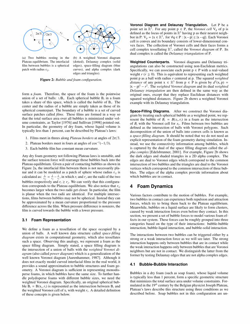
(a) Two bubbles resting in thePlateau equilibrium. The interfacialfilm between bubbles is a sphericalpatch with radius ri j.

(b) A weighted Voronoi diagram(dotted), Delaunay complex (solidedges), space-filling diagram (bluecurves), and alpha complex (darkedges and triangles).

Figure 2: Bubble and foam configuration.

form a foam. Therefore, the space of the foam is the pointwiseunion of a set of balls: ∪Bi. Each spherical bubble Bi in a foamtakes a share of this space, which is called the bubble of Bi. Thecenter and the radius of a bubble are simply taken as those of itsspherical counterpart. The boundary of a bubble is a set of curvedsurface patches called films. These films are formed in a way sothat the total surface area over all bubbles is minimized under vol-ume constraints, as Taylor [1976] and Sullivan [1998] pointed out.In particular, the geometry of dry foam, whose liquid volume istypically less than 1 percent, can be described by Plateau’s laws:

1. Films meet in threes along Plateau borders at angles of 2π/3.2. Plateau borders meet in fours at angles of cos−1(−1/3).3. Each bubble film has constant mean curvature.

Any dry foam geometry not following Plateau laws is unstable, andthe surface tension force will rearrange those bubbles back into thePlateau equilibrium. Given a pair of contacting bubbles as shown inFigure 2a, the interfacial film between them is not necessarily pla-nar and it can be modeled as a patch of sphere whose radius ri j iscalculated as: 1

ri j= 1

r j− 1

ri, in which ri and r j are the radii of the two

bubbles respectively and ri ≥ r j. We can verify that this configura-tion corresponds to the Plateau equilibrium. We also notice that ri jbecomes larger when the two radii get closer. In particular, the filmis planar when the two radii are identical. For multiple intersec-tions, films between bubbles may not be spherical. Instead they canbe approximated by a mean curvature proportional to the pressuredifference across the film. When pressure difference is nonzero, thefilm is curved towards the bubble with a lower pressure.

3.1 Foam Representation

We define a foam as a tessellation of the space occupied by aunion of balls. A well known data structure called space-fillingdiagram exists in computational geometry, which also tessellatessuch a space. Observing this analogy, we represent a foam as thespace filling diagram. Simply stated, a space filling diagram isthe intersection of a union of balls with the weighted Voronoi di-agram (also called power diagram) which is a generalization of thewell known Voronoi diagram [Aurenhammer, 1987]. Although itdoes not exactly model curved interfacial films in the real world, itprovides a sound approximation to bubble structures and foam ge-ometry. A Voronoi diagram is sufficient in representing monodis-perse foams, in which bubbles have the same size. To further han-dle polydisperse foams with different bubble sizes, we need theweighted Voronoi diagram. Specifically, an original spherical bub-ble Bi = B(xi, ri) is represented as the intersection between Bi andthe weighted Voronoi cell of xi with weight ri. A detailed definitionof these concepts is given below.

Voronoi Diagram and Delaunay Triangulation. Let P be apoint set in R3. For any point p ∈ P, the Voronoi cell Vp of p isdefined as the locus of points in R3 having p as their nearest neigh-bor in P: Vp = {x ∈ R3, for ∀q ∈ P : |x−p| ≤ |x−q|}. Each Voronoicell is convex and its boundary consists of lower-dimensional con-vex faces. The collection of Voronoi cells and their faces forms acell complex tessellating R3, called the Voronoi diagram of P. Itsdual complex is called the Delaunay triangulation of P.

Weighted Counterparts. Voronoi diagrams and Delaunay tri-angulations can also be constructed using non-Euclidean metrics.Specifically, we can associate each point p ∈ P with a real-valuedweight r (r ≥ 0). This is equivalent to representing each weightedpoint p as a ball with radius r centered at p. The squared weighteddistance of any point x ∈ R3 from p ∈ P is given by d2(x, p) =|x − p|2 − r2. The weighted Voronoi diagram and its dual weightedDelaunay triangulation are then defined in the same way as theoriginal ones, except that they replace Euclidean distances withsquared weighted distances. Figure 2b shows a weighted Voronoiexample with its Delaunay triangulation.

Space-Filling Diagrams. After we construct the Voronoi dia-gram by treating each spherical bubble as a weighted point, we rep-resent the bubble of Bi = B(xi, ri) in a foam as the intersectionof Bi with the Voronoi cell for xi. Films between two bubbles aredefined as the intersection of balls with Voronoi polygons. Suchdecomposition of the union of balls into convex cells is known asa space-filling diagram. It should be noted that we do not need anexplicit representation of the foam geometry during simulation. In-stead, we use the connectivity information among bubbles, whichis captured by the dual of the space filling diagram called the al-pha complex [Edelsbrunner, 2001]. For example, Figure 2b showsthe dark edges and shaded triangles in a 2D alpha complex. Theedges are dual to Voronoi edges which correspond to the commonintersection of two bubbles and the triangles are dual to the Voronoivertices which correspond to the common intersection of three bub-bles. The edges of the alpha complex provide information aboutwhich bubbles are in contact.

4 Foam Dynamics

Various factors contribute to the motion of bubbles. For example,two bubbles in contact can experience both repulsion and attractionforces, which try to bring them back to the Plateau equilibrium.Meanwhile, bubbles on a liquid surface are likely to form clusters,caused by weak interaction forces even before they contact. In thissection, we present a set of bubble forces to model various foam ef-fects in our system. These forces can be roughly grouped into threecategories based on the type of their interactions: bubble-bubbleinteraction, bubble-liquid interaction, and bubble-solid interaction.

The interactions between two bubbles can be triggered either by astrong or a weak interaction force as we will see later. The stronginteraction happens only between bubbles that are in contact whilethe weak interaction happens only between bubbles that are Voronoineighbors but are not in contact. We distinguish the latter from theformer by testing Delaunay edges that are not alpha complex edges.

4.1 Bubble-Bubble Interaction

Bubbles in a dry foam (such as soap foam), whose liquid volumeis typically less than 1 percent, form a specific geometric structurethat minimizes the total surface area under volume constraints. For-mulated in the 19th century by the Belgian physicist Joseph Plateau,Plateau’s laws describe this structure using three conditions as wedescribed before. Soap bubbles not in this configuration are un-

φ < 0

φ > 0a

c

b

dgf

e

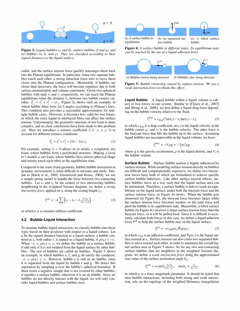
Figure 3: Liquid bubbles (c and d), surface bubbles (f and g), andair bubbles (a, b, and e). They are classified according to theirsigned distances to the liquid surface.

stable, and the surface tension force quickly rearranges them backinto the Plateau equilibrium. In particular, when two separate bub-bles touch each other, a strong attraction force tries to move themcloser into the Plateau configuration. Meanwhile, if bubbles arecloser than necessary, the force will become repulsive due to bothsurface minimization and volume constraints. Given two sphericalbubbles with radii ri and r j respectively, we can reach the Plateauequilibrium when the distance li j between two bubble centers sat-isfies: l2

i j = r2i + r2

j − rir j. Figure 2a shows such an example, inwhich bubble films form 2π/3 angles according to Plateau’s laws.This condition also provides a reasonable approximation for mul-tiple bubble cases. However, it becomes less valid for wet foams,in which the extra liquid in interfacial films can affect the surfacetension. Unfortunately, the geometric structure of wet foam is morecomplex, and no clear conclusions have been made to this problemyet. Here we introduce a wetness coefficient λ (1 ≤ λ ≤ 1) toaccount for different wetness conditions:

l2i j = r2

i + r2j + (3λ − 1)rir j. (1)

For example, setting λ = 0 allows us to mimic a completely dryfoam, where bubbles form a polyhedral structure. Making λ closeto 1 models a wet foam, where bubbles have almost spherical shapeand merely touch each other in the equilibrium state.

Compared to the static foam geometry, bubble-bubble interaction indynamic environment is more difficult to measure and study. Sim-ilar to [Kuck et al., 2002; Greenwood and House, 2004], we usea simple spring model to handle the force between two contactingbubbles. Let xi and x j be the centers of two intersecting bubblesneighboring in the weighted Voronoi diagram, we define a stronginteraction force applied on xi using the resting length li j:

fsinti = −k

∑j

(xi − x j − li j

xi−x j

|xi−x j|

), (2)

in which k is a constant stiffness coefficient.

4.2 Bubble-Liquid Interaction

To simulate bubble-liquid interaction, we classify bubbles into threetypes based on their positions with respect to a liquid volume. Letϕ be the signed distance function to a liquid surface, a bubble cen-tered at xi with radius ri is named as a liquid bubble, if ϕ(xi) < −ri.When −ri ≤ ϕ(xi) ≤ ri, we define the bubble as a surface bubble,if and only if it is not isolated from the liquid surface by other bub-bles. The rest of bubbles are called air bubbles. Figure 3 showsan example, in which bubbles e, f, and g all satisfy the condition:−ri ≤ ϕ(xi) ≤ ri. However, bubble e is still an air bubble, sinceit is separated from the liquid by bubble f and g. We detect thisseparation by sampling ϕ over the bubble’s spherical boundary. Ifthere exists a negative sample that is not covered by other bubbles,it signifies a surface bubble, otherwise it is an air bubble. Since airbubbles do not directly interact with the liquid, we will only con-sider liquid bubbles and surface bubbles next.

f lad

f lad

(a) A surface bubble inequilibrium

(b) An immersed sur-face bubble

(c) A lifted surfacebubble

Figure 4: A surface bubble in different states. Its equilibrium statecan be reached by the use of a liquid adhesion force.

f wint f wint

(a) Bubbles before being attracted (b) Bubbles after being attracted

Figure 5: Bubble clustering caused by surface tension. We use aweak interaction force to obtain this effect.

Liquid Bubble. A liquid bubble within a liquid volume is sub-ject to two forces in our system. Similar to [Cleary et al., 2007]and [Hong et al., 2008], we first define a liquid drag force depend-ing on the bubble velocity relative to the fluid:

fdragi = cdragr2

i (u(xi) − vi)|u(xi) − vi|, (3)

in which cdrag is a drag coefficient, u(xi) is the liquid velocity at thebubble center xi, and vi is the bubble velocity. The other force isthe buoyant force that lifts the bubble up to the surface. Assumingliquid bubbles are incompressible in the liquid volume, we have:

fbuoyi = −Viρg = − 4

3πr3i ρg. (4)

where g is the gravity acceleration, ρ is the liquid density, and Vi isthe bubble volume.

Surface Bubble. Surface bubble motion is highly influenced bysurface tension. While modeling surface tension directly on bubblesare difficult and computationally expensive, we define two interac-tion forces here, both of which are formulated to achieve specificsurface bubble behaviors. Like other surface tension effects, sur-face bubbles move in a way such that the liquid surface area canbe minimized. Therefore, a surface bubble is able to reach an equi-librium on the liquid surface, under both the buoyant force and thesurface tension force, as Figure 4a shows. When the bubble getsimmersed (in Figure 4b), the buoyant force becomes larger whilethe surface tension force becomes weaker, so the total force willpush the bubble to its equilibrium state. Meanwhile, a lifted surfacebubble (in Figure 4c) receives a larger surface tension force than thebuoyant force, so it will be pulled back. Since it is difficult to accu-rately calculate both forces in this case, we define a liquid adhesionforce flad to help the surface bubble stay on the liquid surface:

fladi = −σladϕ(xi)∇ϕ(xi), (5)

in which σlad is an adhesion coefficient, and ∇ϕ(xi) is the liquid sur-face normal at xi. Surface tension can also cause two separated bub-bles to move toward each other, in order to minimize the overall liq-uid surface area as Figure 5 shows. So for any two non-contactingsurface bubbles that are neighbors in the weighted Voronoi dia-gram, we define a weak interaction force using the approximatedsine value of the surface inclination angle θi j:

fwinti j = α sin θi j

x j−xi|x j−xi |

, sin θi j =r j

|xi−x j |, (6)

in which α is a force magnitude parameter. It should be noted thatinter-bubble interactions, including both strong and weak interac-tion, rely on the topology of the weighted Delaunay triangulation

(or its dual weighted Voronoi diagram). Delaunay edges that belongto the alpha complex indicate strong interaction forces for contact-ing bubbles, while the remaining Delaunay edges help us formulateweak interaction forces for surface bubbles.

4.3 Bubble-Solid Interaction

In order to model the hydrophilicity of certain solid objects, we usean adhesion force to prevent bubbles from leaving solid surfaces:

fsadi = −σsadψ(xi)∇ψ(xi), (7)

in which σsad is an adhesion coefficient and ψ(xi) gives the signeddistance from the bubble center xi to the solid. The adhesion forceacts on each bubble that has ever touched the solid. In addition, wedefine a solid attraction force to move surface bubbles closer to thesolid, due to a similar surface minimization reason we discussedbefore in Subsection 4.2:

fsati = −β∇ψ/|ψ|, (8)

in which β is a solid attraction coefficient.

5 Foam Simulation

Based on foam representation and foam dynamics presented in Sec-tion 3 and 4 respectively, we develop a foam simulator to updatebubbles and foams in each time step. It first uses an implicit inte-grator to evolve bubble positions and velocities, according to foamdynamics. It then applies a volume conservation constraint to com-pensate the bubble volume loss during simulation, especially whenbubbles are heavily squeezed. Finally, we perform topological up-dates on the foam structure and reconstruct the weighted Voronoidiagram, to ensure that it remains valid for further simulation.

5.1 Time Integrator

We use the implicit solver proposed by Baraff and Witkin [1998] toevolve bubble particles over time. Given bubble positions {xt

i} andvelocities {vt

i} at time t, the solver uses the backward Euler methodto compute bubble velocities {vt+1

i } at the next time step:(M − ∆t∂ft/∂v − ∆t2∂ft/∂x

)vt+1 = Mvt + ∆tft, (9)

in which M is a mass matrix, ∆t is the time step, and f, x and vare vectors of bubble forces, positions, and velocities respectively.The force vector f is made of the gravity force, the air dampingforce, and the total interaction force. The gravity force fgrav

i = migon bubble i is independent of bubble position and velocity, so itsJacobian matrices ∂fgrav/∂x and ∂fgrav/∂v are both zero matrices.We define the damping force using two damping coefficients (cvisand clap) and a normalized Laplacian matrix L: fdamp = −cvisv −clapLv. Its Jacobian matrix can be written as:

ci j =

−(cvis + clap)I, for i = j

clap

(|Ni|

∣∣∣N j

∣∣∣)−1/2I, for i , j and i ∈ N j

0, otherwise(10)

in which ci j is a 3×3 sub-matrix, and Ni is the 1-ring contact neigh-borhood of vertex i, given by the weighted Voronoi diagram. Theoverall interaction force is the sum of three interaction forces dis-cussed in Section 4. Most interaction forces are comparably small,so they can be treated explicitly by simply ignoring their Jacobianmatrices. The only exception is the strong bubble interaction forcemodeled by a stiff spring in Equation 4. Similar to the formula pro-posed by Choi and Ko [2002], we use Taylor expansion to find the

Jacobian matrix of fsint respect to x. We also drop the geometricterm when the spring is compressed, to ensure numerical stability.

The linear system in Equation 11 is guaranteed to be symmetricpositive definite. We solve it using the Preconditioned ConjugateGradient (PCG) method with an incomplete Cholesky precondi-tioner. Since interaction forces in our method depend on bubbleconnectivity that may vary over time, the whole system is not un-conditionally stable. Fortunately, our experiment shows that thesystem can robustly handle large time steps (∆t ∈ [0.005s, 0.02s])for most examples without any oscillation artifacts.

5.2 Volume Correction

The weighted Voronoi diagram changes when bubble move. Asa result, some bubbles represented by the cells of the space-fillingdiagram may experience considerable volume changes. To preservethe bubble volume, we perform a volume correction step.

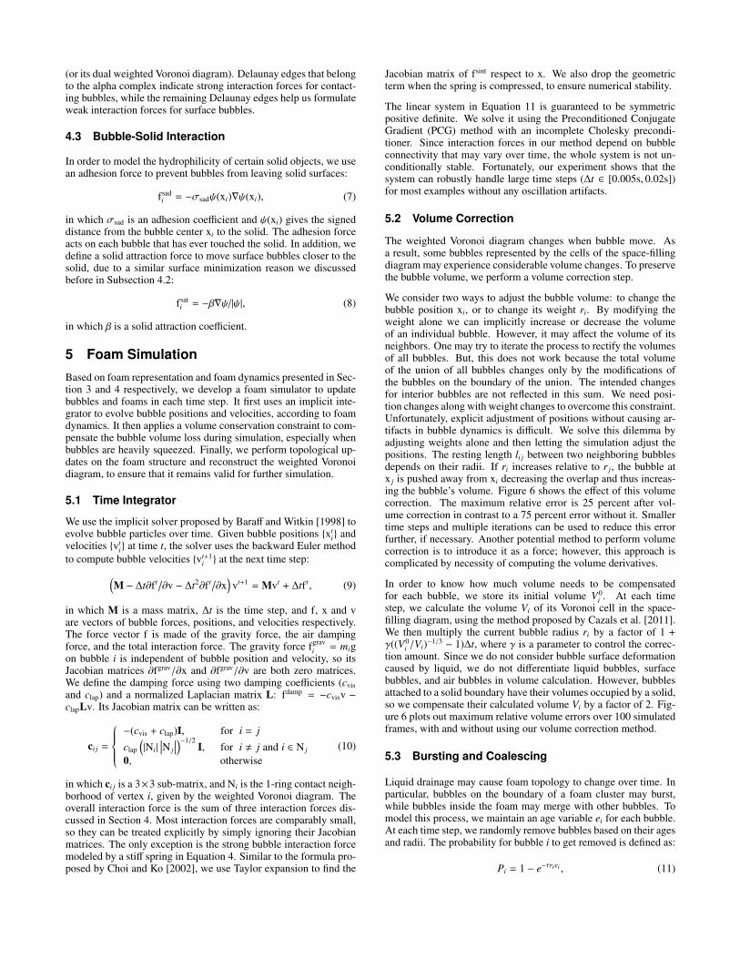
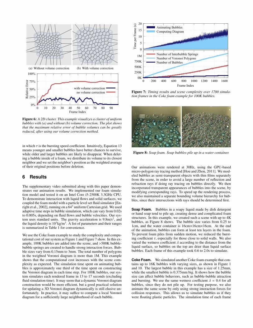
We consider two ways to adjust the bubble volume: to change thebubble position xi, or to change its weight ri. By modifying theweight alone we can implicitly increase or decrease the volumeof an individual bubble. However, it may affect the volume of itsneighbors. One may try to iterate the process to rectify the volumesof all bubbles. But, this does not work because the total volumeof the union of all bubbles changes only by the modifications ofthe bubbles on the boundary of the union. The intended changesfor interior bubbles are not reflected in this sum. We need posi-tion changes along with weight changes to overcome this constraint.Unfortunately, explicit adjustment of positions without causing ar-tifacts in bubble dynamics is difficult. We solve this dilemma byadjusting weights alone and then letting the simulation adjust thepositions. The resting length li j between two neighboring bubblesdepends on their radii. If ri increases relative to r j, the bubble atx j is pushed away from xi decreasing the overlap and thus increas-ing the bubble’s volume. Figure 6 shows the effect of this volumecorrection. The maximum relative error is 25 percent after vol-ume correction in contrast to a 75 percent error without it. Smallertime steps and multiple iterations can be used to reduce this errorfurther, if necessary. Another potential method to perform volumecorrection is to introduce it as a force; however, this approach iscomplicated by necessity of computing the volume derivatives.

In order to know how much volume needs to be compensatedfor each bubble, we store its initial volume V0

i . At each timestep, we calculate the volume Vi of its Voronoi cell in the space-filling diagram, using the method proposed by Cazals et al. [2011].We then multiply the current bubble radius ri by a factor of 1 +γ((V0

i /Vi)−1/3 − 1)∆t, where γ is a parameter to control the correc-tion amount. Since we do not consider bubble surface deformationcaused by liquid, we do not differentiate liquid bubbles, surfacebubbles, and air bubbles in volume calculation. However, bubblesattached to a solid boundary have their volumes occupied by a solid,so we compensate their calculated volume Vi by a factor of 2. Fig-ure 6 plots out maximum relative volume errors over 100 simulatedframes, with and without using our volume correction method.

5.3 Bursting and Coalescing

Liquid drainage may cause foam topology to change over time. Inparticular, bubbles on the boundary of a foam cluster may burst,while bubbles inside the foam may merge with other bubbles. Tomodel this process, we maintain an age variable ei for each bubble.At each time step, we randomly remove bubbles based on their agesand radii. The probability for bubble i to get removed is defined as:

Pi = 1 − e−τriei , (11)

(a) Without volume correction (b) With volume correction

0%

25%

50%

75%

100%

0 10 20 30 40 50 60 70 80 90

Rel

ativ

e E

rror

Frame Index

with volume correctionno volume correction

Figure 6: A 2D cluster. This example visualizes a cluster of uniformbubbles with (a) and without (b) volume correction. The plot showsthat the maximum relative error of bubble volumes can be greatlyreduced, after using our volume correction method.

in which τ is the bursting speed coefficient. Intuitively, Equation 13means younger and smaller bubbles have better chances to survive,while older and larger bubbles are likely to disappear. When delet-ing a bubble inside of a foam, we distribute its volume to its closestneighbor and we set the neighbor’s position as the weighted averageof their original positions before deletion.

6 Results

The supplementary video submitted along with this paper demon-strates our animation results. We implemented our foam simula-tion model and tested it on an Intel Core i5-2500K 3.3GHz CPU.To demonstrate interaction with liquid flows and solid surfaces, wecoupled the foam model with a particle level set fluid simulator [En-right et al., 2002], running on a 643 uniform Cartesian grid. We usedadaptive time steps in bubble simulation, which can vary from 0.02sto 0.005s, depending on fluid flows and bubble velocities. Our sys-tem uses standard units. The gravity acceleration is 9.8m/s2, andthe liquid density is 103kg/m3. A list of parameters and their rangesis summarized in Table 1 for convenience.

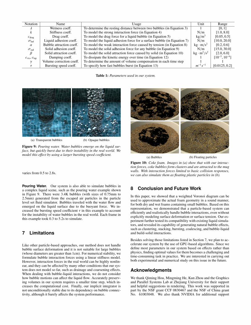
We use the Coke foam example to study the complexity and compu-tational cost of our system as Figure 1 and Figure 7 show. In this ex-ample, 100K bubbles are added into the scene, and >500K bubble-bubble springs are created to handle strong interaction forces. Bub-ble sizes vary from 0.15mm to 3mm. The total number of polygonsin the weighted Voronoi diagram is more than 1M. This exampleshows that the computational cost increases with the scene com-plexity as expected. The simulation time spent on animating bub-bles is approximately one third of the time spent on constructingthe Voronoi diagram in each time step. For 100K bubbles, our sys-tem simulates each rendered frame in 13 to 17 seconds (excludingfluid simulation time). It may seem that a dynamic Voronoi diagramconstruction would be more efficient, but a good practical solutionfor updating a 3D Voronoi diagram dynamically is still elusive un-fortunately. In practice, it may suffice to compute a local Voronoidiagram for a sufficiently large neighborhood of each bubble.

0

5

10

15

20

Tim

e pe

r F

ram

e (s

)

Animating BubblesComputing Diagram

0K

250K

500K

750K

1M

0 200 400 600 800 1000 1200 1400 1600

Frame Index

Number of Interbubble SpringsNumber of Voronoi PolygonsNumber of Bubbles

Figure 7: Timing results and scene complexity over 1700 simula-tion frames in the Coke foam example for 100K bubbles.

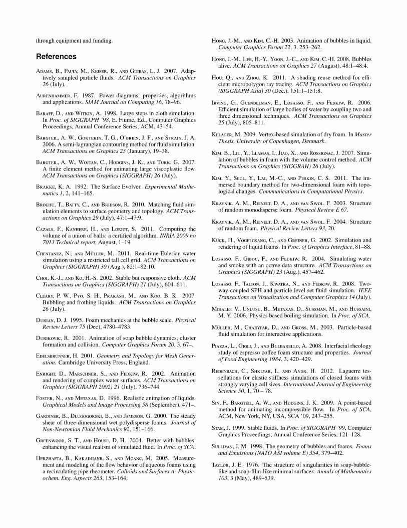
Figure 8: Soap foam. Soap bubbles pile up in a water container.

Our animations were rendered at 30Hz, using the GPU-basedmicro-polygon ray tracing method [Hou and Zhou, 2011]. We mod-eled bubbles as semi-transparent objects with thin films separatelyfrom the scene, in order to avoid a large number of reflection andrefraction rays if doing ray tracing on bubbles directly. We thenincorporated transparent appearances of bubbles into the scene, bymodifying corresponding rays. To speed up the rendering process,we also maintained a separate bounding volume hierarchy for bub-bles, since their intersections with rays should be determined first.

Soap Foam. Bubbles in a soapy liquid made by dish detergentor hand soap tend to pile up, creating dense and complicated foamstructures. In this example, we created such a scene with up to 4Kbubbles, as Figure 8 shows. The bubble size varies from 0.25 to1cm, and the water container is 16cm×16cm×16cm. At the endof the animation, bubbles can form at least ten layers in the foam.To prevent foam piles from sudden motion, we reduced the burst-ing coefficient τ, especially for those close to solid walls. We alsovaried the wetness coefficient λ according to the distance from theliquid surface, so bubbles on the top are drier than liquid surfacebubbles. Each frame of this example took 0.6 to 2.0s to simulate.

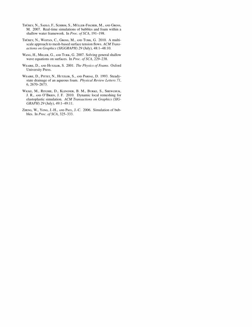
Coke Foam. We simulated another Coke foam example that con-tains up to 16K bubbles with varying sizes, as shown in Figure 1and 10. The largest bubble in this example has a size of 1.25mm,while the smallest bubble is 0.375mm big. It shows how the bubblesize can affect bubble behaviors, such as bubble-bubble attractionand bursting. We use the same wetness coefficient λ = 0.4 for allbubbles, since they do not pile up. For testing purpose, we alsoanimate the same scene by only using strong interaction forces forcollision responses. This allows us to simulate bubbles as if theywere floating plastic particles. The simulation time of each frame

Notation Name Usage Unit Rangeλ Wetness coeff. To determine the resting distance between two bubbles (in Equation 3) 1 [0, 1]k Stiffness coeff. To model the strong interaction force (in Equation 4) N/m [1.0, 8.0]

cdrag Drag coeff. To model the drag force for a liquid bubble (in Equation 5) kg/m3 [0.05, 0.5]σlad Liquid adhesion coeff. To model the liquid adhesion force for a surface bubble (in Equation 7) N/m [10.0, 20.0]α Bubble attraction coeff. To model the weak interaction force caused by tension (in Equation 8) kg ·m/s2 [0.2, 0.6]σsad Solid adhesion coeff. To model the solid adhesion force for any bubble (in Equation 9) N/m [15.0, 30.0]β Solid attraction coeff. To model the solid attraction force caused by solid (in Equation 10) kg ·m2/s2 [2.0, 6.0]

cvis, clap Damping coeff. To dissipate the kinetic energy over time (in Equation 12) 1 [10−5, 10−4]γ Volume correction coeff. To determine the amount of volume compensation in each time step 1 1τ Bursting speed coeff. To specify how fast bubbles burst (in Equation 13) m−1 s−1 [0.0125, 0.2]

Table 1: Parameters used in our system.

(a) Transparent bubbles (b) Opaque bubbles

Figure 9: Pouring water. Water bubbles emerge on the liquid sur-face, but quickly burst due to their instability in the real world. Wemodel this effect by using a larger bursting speed coefficient.

varies from 0.5 to 2.8s.

Pouring Water. Our system is also able to simulate bubbles ina complex liquid scene, such as the pouring water example shownin Figure 9. There were 3.4K bubbles (with sizes of 0.75mm to2.5mm) generated from the escaped air particles in the particlelevel set fluid simulator. Bubbles traveled with the water flow andemerged on the liquid surface due to the buoyant force. We in-creased the bursting speed coefficient τ in this example to accountfor the instability of water bubbles in the real world. Each frame inthis example took 0.3 to 5.2s to simulate.

7 Limitations

Like other particle-based approaches, our method does not handlebubble surface deformation and it is not suitable for large bubbles(whose diameters are greater than 1cm). For numerical stability, weformulate bubble interaction forces using a linear stiffness model.However, interaction forces in the real world can be highly nonlin-ear, and they can be affected by many other conditions that our sys-tem does not model so far, such as drainage and coarsening effects.When dealing with bubble-liquid interactions, we do not considerhow bubble motions can affect the liquid flow. Accurately preserv-ing volumes in our system requires a smaller time step, which in-creases the computational cost. Finally, our implicit integrator isnot unconditionally stable due to its dependency on bubble connec-tivity, although it barely affects the system performance.

(a) Bubbles (b) Floating particles

Figure 10: Coke foam. Images in (a) show that with our interac-tion forces, coke bubbles form clusters and are attracted to the mugwalls. With interaction forces limited to basic collision responses,we can also simulate them as floating plastic particles in (b).

8 Conclusion and Future Work

In this paper, we showed that a weighted Voronoi diagram can beused to approximate the actual foam geometry in a sound manner,for both dry and wet foams containing small bubbles. Based on thisrepresentation, we demonstrated that a particle-based system canefficiently and realistically handle bubble interactions, even withoutexplicitly modeling surface deformation or surface tension. Our ex-periment further tested its compatibility with existing liquid simula-tors, and revealed its capability of generating natural bubble effects,such as clustering, stacking, bursting, coalescing, and bubble-liquidand build-solid interactions.

Besides solving those limitations listed in Section 7, we plan to ac-celerate our system by the use of GPU-based algorithms. Since wedefine most parameters in our system based on effects rather thanphysics, finding optimal values for them becomes a challenging andtime-consuming task in practice. We are interested in carrying outboth experimental and numerical study on this issue in the future.

Acknowledgments

We thank Qiming Hou, Mingming He, Kun Zhou and the Graphicsand Parallel Systems Lab at Zhejiang University for their supportand helpful suggestions in rendering. This work was supported inpart by the NSF grant CCF 0830467 and the NSF of China grantNo. 61003048. We also thank NVIDIA for additional support

through equipment and funding.

References

A, B., P, M., K, R., G, L. J. 2007. Adap-tively sampled particle fluids. ACM Transactions on Graphics26 (July).

A, F. 1987. Power diagrams: properties, algorithmsand applications. SIAM Journal on Computing 16, 78–96.

B, D., W, A. 1998. Large steps in cloth simulation.In Proc. of SIGGRAPH ’98, E. Fiume, Ed., Computer GraphicsProceedings, Annual Conference Series, ACM, 43–54.

B, A. W., G, T. G., O’, J. F., S, J. A.2006. A semi-lagrangian contouring method for fluid simulation.ACM Transactions on Graphics 25 (January), 19–38.

B, A. W., W, C., H, J. K., T, G. 2007.A finite element method for animating large viscoplastic flow.ACM Transactions on Graphics (SIGGRAPH) 26 (July).

B, K. A. 1992. The Surface Evolver. Experimental Mathe-matics 1, 2, 141–165.

B, T., B, C., B, R. 2010. Matching fluid sim-ulation elements to surface geometry and topology. ACM Trans-actions on Graphics 29 (July), 47:1–47:9.

C, F., K, H., L, S. 2011. Computing thevolume of a union of balls: a certified algorithm. INRIA 2009 no7013 Technical report, August, 1–19.

C, N., M, M. 2011. Real-time Eulerian watersimulation using a restricted tall cell grid. ACM Transactions onGraphics (SIGGRAPH) 30 (Aug.), 82:1–82:10.

C, K.-J., K, H.-S. 2002. Stable but responsive cloth. ACMTransactions on Graphics (SIGGRAPH) 21 (July), 604–611.

C, P. W., P, S. H., P, M., K, B. K. 2007.Bubbling and frothing liquids. ACM Transactions on Graphics26 (July).

D, D. J. 1995. Foam mechanics at the bubble scale. PhysicalReview Letters 75 (Dec), 4780–4783.

D, R. 2001. Animation of soap bubble dynamics, clusterformation and collision. Computer Graphics Forum 20, 3, 67–.

E, H. 2001. Geometry and Topology for Mesh Gener-ation. Cambridge University Press, England.

E, D., M, S., F, R. 2002. Animationand rendering of complex water surfaces. ACM Transactions onGraphics (SIGGRAPH 2002) 21 (July), 736–744.

F, N., M, D. 1996. Realistic animation of liquids.Graphical Models and Image Processing 58 (September), 471–.

G, B., D, B., J, G. 2000. The steadyshear of three-dimensional wet polydisperse foams. Journal ofNon-Newtonian Fluid Mechanics 92, 151–166.

G, S. T., H, D. H. 2004. Better with bubbles:enhancing the visual realism of simulated fluid. In Proc. of SCA.

H, B., K, S., M, M. 2005. Measure-ment and modeling of the flow behavior of aqueous foams usinga recirculating pipe rheometer. Colloids and Surfaces A: Physic-ochem. Eng. Aspects 263, 153–164.

H, J.-M., K, C.-H. 2003. Animation of bubbles in liquid.Computer Graphics Forum 22, 3, 253–262.

H, J.-M., L, H.-Y., Y, J.-C., K, C.-H. 2008. Bubblesalive. ACM Transactions on Graphics 27 (August), 48:1–48:4.

H, Q., Z, K. 2011. A shading reuse method for effi-cient micropolygon ray tracing. ACM Transactions on Graphics(SIGGRAPH Asia) 30 (Dec.), 151:1–151:8.

I, G., G, E., L, F., F, R. 2006.Efficient simulation of large bodies of water by coupling two andthree dimensional techniques. ACM Transactions on Graphics25 (July), 805–811.

K, M. 2009. Vertex-based simulation of dry foam. In MasterThesis, University of Copenhagen, Denmark.

K, B., L, Y., L, I., J, X., R, J. 2007. Simu-lation of bubbles in foam with the volume control method. ACMTransactions on Graphics (SIGGRAH) 26 (July).

K, Y., S, Y., L, M.-C., P, C. S. 2011. The im-mersed boundary method for two-dimensional foam with topo-logical changes. Communications in Computational Physics.

K, A. M., R, D. A., S, F. 2003. Structureof random monodisperse foam. Physical Review E 67.

K, A. M., R, D. A., S, F. 2004. Structureof random foam. Physical Review Letters 93, 20.

K, H., V, C., G, G. 2002. Simulation andrendering of liquid foams. In Proc. of Graphics Interface, 81–88.

L, F., G, F., F, R. 2004. Simulating waterand smoke with an octree data structure. ACM Transactions onGraphics (SIGGRAPH) 23 (Aug.), 457–462.

L, F., T, J., K, N., F, R. 2008. Two-way coupled SPH and particle level set fluid simulation. IEEETransactions on Visualization and Computer Graphics 14 (July).

M, V., U, B., M, D., S, M., H,M. Y. 2006. Physics based boiling simulation. In Proc. of SCA.

M, M., C, D., G, M., 2003. Particle-basedfluid simulation for interactive applications.

P, L., G, J., B, A. 2008. Interfacial rheologystudy of espresso coffee foam structure and properties. Journalof Food Engineering 1984, 3, 420–429.

R, C., S, I., A, H. 2012. Laguerre tes-sellations for elastic stiffness simulations of closed foams withstrongly varying cell sizes. International Journal of EngineeringScience 50, 1, 70 – 78.

S, F., B, A. W., H, J. K. 2009. A point-basedmethod for animating incompressible flow. In Proc. of SCA,ACM, New York, NY, USA, SCA ’09, 247–255.

S, J. 1999. Stable fluids. In Proc. of SIGGRAPH ’99, ComputerGraphics Proceedings, Annual Conference Series, 121–128.

S, J. M. 1998. The geometry of bubbles and foams. Foamsand Emulsions (NATO ASI volume E) 354, 379–402.

T, J. E. 1976. The structure of singularities in soap-bubble-like and soap-film-like minimal surfaces. Annals of Mathematics103, 3 (May), 489–539.

T, N., S, F., S, S., M-F, M., G,M. 2007. Real-time simulations of bubbles and foam within ashallow water framework. In Proc. of SCA, 191–198.

T, N., W, C., G, M., T, G. 2010. A multi-scale approach to mesh-based surface tension flows. ACM Trans-actions on Graphics (SIGGRAPH) 29 (July), 48:1–48:10.

W, H., M, G., T, G. 2007. Solving general shallowwave equations on surfaces. In Proc. of SCA, 229–238.

W, D., H, S. 2001. The Physics of Foams. OxfordUniversity Press.

W, D., P, N., H, S., P, D. 1993. Steady-state drainage of an aqueous foam. Physical Review Letters 71,6, 2670–2673.

W, M., R, D., K, B. M., B, S., S,J. R., O’B, J. F. 2010. Dynamic local remeshing forelastoplastic simulation. ACM Transactions on Graphics (SIG-GRAPH) 29 (July), 49:1–49:11.

Z, W., Y, J.-H., P, J.-C. 2006. Simulation of bub-bles. In Proc. of SCA, 325–333.