Advanced Studies in Pure Mathematics 99, 20XX

Title

pp. 1–30

Anisotropic Diffusions of Image ProcessingFrom Perona-Malik on

Patrick Guidotti

Abstract.

Many reasons can be cited for the desire to harness thepower of nonlinear anisotropic diffusion in image processing.Perona and Malik proposed one of the pioneering models which,while numerically viable, proves mathematically ill-posed. Thisdiscrepancy between its analytical properties and those of itsnumerical implementations spurred a significant amount of re-search in the past twenty years or so. An overview of the latteris the topic of this article.

§1. Introduction

Mathematical image processing was profoundly influenced bythe introduction of two prototypical models in the late 80ies, early90ies: Mumford-Shah [60] and Perona-Malik [62]. The first is avariational model as it is formulated by means of the functional

(1) EMS(u,Γ) =1

2

∫Ω\Γ|∇u|2 dx+ α

∫Ω|Ku− u0|2 dx+ βl(Γ) ,

where a possibly non-smooth minimizer u is sought for which thelength l(Γ) of its discontinuity set Γ, in a typical two dimensionalsetting, is penalized. Away from the set Γ, the first terms enforcessmoothness, while the second penalizes overall deviation from theobserved data u0. The smoothing operator K models any blurringpresent in the image. When K = id, one deals with the “pure”

Key words and phrases. Anisotropic diffusion, Perona-Malik equa-tion, regularization, relaxation, semi-discretization, forward-backwarddiffusion, gradient systems.

2 P. Guidotti

denoising problem. The second model, while at least formally thegradient flow associated to

(2) EPM (u) =1

2

∫Ω

log(1 + |∇u|2

)dx ,

is best viewed as an example of forward-backward diffusion in viewof the convex-concave nature of

(3) ϕ(s) =1

2log(1 + |s|2) , s ∈ R2 .

The corresponding PDE reads

(4) ut = ∇ ·( 1

1 + |∇u|2∇u)

=1

1 + |∇u|2(∂ττu+

1− |∇u|2

1 + |∇u|2∂νν),

and clearly allows for backward diffusion in direction ν normal tothe level sets of the function u for large enough gradients, whilealways maintaining a forward nature in tangential direction(s) τ .For this very reason, equation (4) is customarily become labeledas a, if not the example of, anisotropic diffusion. The two mod-els above, or related ones derived from them, are typically usedfor so-called low level image processing tasks such as denoising,deblurring, or segmentation, to name only the most common. Insuch a context, u0 represents a given image which needs to be en-hanced (read denoised, deblurred, or segmented, respectively). Itexplicitly appears in (1) and enters into (4) as the initial conditionfor the Cauchy problem. The Mumford-Shah model (1) presentsnon-trivial numerical challenges and has therefore lead to a varietyof approximations (often in the sense of Γ-convergence) includingan early one by Ambrosio and Tortorelli [3] which replaces theperimeter term by an approximating bulk integral. It is, in a way,remarkable that, on the contrary, the Perona-Malik model (4)poses significant mathematical challenges while delivering betterbehaved numerical implementations than expected.

The focus of this overview paper is on anisotropic diffusionand no further mention will be made of the numerous subsequentdevelopments in the variational arena revolving around or inspiredby the Mumford and Shah model. It is only pointed out in passingthat a, at least formal, connection between (1) and (4) was found

Anisotropic Diffusions 3

by Chan and Vese [19] (see also the overview article by Kawohl[53]).

In the early 90ies Perona and Malik [62] proposed a nonlinearmodel for image processing in order to replace/improve on previ-ous techniques based on linear filtering followed by edge identifi-cation and reconstruction. Linear filtering essentially amounts tosolving a linear heat equation

ut = ∆u ,

u(0, ·) = u0 ,

whereas the second phase requires an edge detector typically basedon the use of |∇u| or |∆u| such as is the case for the Canny or forthe Marr-Hildreth edge detectors [16, 59]. Perona and Malik’s ideaconsisted in combining the two steps into a single one by integrat-ing edge detection into a nonlinear diffusion equation modulatedby a diffusivity varying according to the local geometric featuresof the image. While they actually consider a discrete model intheir paper, its “apparent” continuos counterpart has come to beknown as the Perona-Malik equation. For the sake of complete-

ness it should be mentioned that they also considered e−|∇u|2

asan alternative diffusivity function and that only the qualitativebehavior of the flux function ∇ϕ really matters. For this reasononly (3) is considered in this paper. Perona and Malik observe in[62] that “solutions” should, contrary to the case of linear back-ward diffusion, satisfy a maximum principle, thus excluding thepossibility of L∞-instability. This is later proved to be true forweak C1-solutions by Kawohl and Kutev [54] and independentlyby Weickert [72]. The existence of a backward regime, however,makes (4) ill-posed. A fact that was first formalized in a paper byKichenassamy [55] in 1996.

Numerical experiments strongly suggest that the ill-posednessof (4) manifests itself through the staircasing effect, so-called forits characteristic appearance (see Figure 1). In the interveningyears after the original publication of [62] many attempts weremade to either

- gain a satisfactory understanding of (4).- find well-posed models preserving salient features of (4).

4 P. Guidotti

0 0.1 0.2 0.3 0.4 0.5 0.6 0.7 0.8 0.9 1−300

−200

−100

0

100

200

300

Plot of ux(2,⋅)

x

0 0.1 0.2 0.3 0.4 0.5 0.6 0.7 0.8 0.9 1−5

0

5

Plot of u0 and u(2,⋅)

x

u(2,⋅)u

0

Fig. 1. A typical manifestation of staircasing. De-picted are an inital datum u0 and the solutionu(t, ·) of (4) at t = 2.

- produce a mathematically sound “rationale” for the be-havior of typical solutions observed in numerical experi-ments.

The rest of the paper is devoted to providing a representative(albeit possibly incomplete) overview of these attempts.

§2. Results about the Perona-Malik equation

While the Perona-Malik equation is an example of a forward-backward diffusion and, as such, it is ill-posed, its instability doesnot manifest itself at the level of the function values of its solutionssince

(5) ‖u(t, ·)‖∞ ≤ ‖u0‖∞ , t > 0 ,

as was proved in [54] and was already mentioned above. Numericalexperiments strongly suggest that ill-posedness affects the behav-ior of the gradient of the solution leading to the staircasing phe-nomenon. The equation possesses, however, a classical regime inwhich solutions are smooth and converge to a trivial steady-state.It indeed follows from the maximum principle [54, Theorem 6.1]

Anisotropic Diffusions 5

that a solution, which is initially subcritical, satisfies

‖∇u(t, ·)‖∞ ≤ ‖∇u0‖∞ , t > 0 ,

and thus remains subcritical for all times. A function is calledsubcritical if its gradient is (everywhere) in the forward regime[|s| < 1] of the equation. If it exhibits non-trivial regions bothin the backward and forward regimes of the equation it is calledtranscritical. A proof of the ill-posedness of was formalized byKichenassamy in [55], where he showed that a solution can onlyexist (in general) for a transcritical initial datum if it is very spe-cial (read very smooth). Most of the early results obtained for thePerona-Malik equation pertain the one dimensional case. Theywill be described first. Kichenassamy proposed a concept of gen-eralized solution for the one-dimensional version (4) which wouldinclude piecewise smooth functions and would allow piecewise con-stant functions, in particular, to be considered stationary for theevolution. This would provide some intuitive, if not rigorous andquantitative, explanation for the generic staircasing behavior ofsolutions. The definition of generalized solution used relies, how-ever, on taking a limit of solutions in which the equation goeslost. More precisely, a Lipschitz continuous function u : U → R isa generalized solution according to [55] of

P (u) := ut − ∂x( 1

1 + |∂xu|2∂xu)

=: ut − ∂xR(∂xu) = 0

if an approximating sequence (un)n∈N exists such that

(6)

un → u in L1

loc(U)

R(∂xun) R(∂xu) in L2(U)

P (un) 0 in D′(U)

, as n→∞ .

According to this definition, piecewise constant functions are gen-eralized steady-states. In particular, this would indicate that thelocation of discontinuity points do not migrate with time. This isin contrast with the behavior of generalized solutions of (4) whichare piecewise smooth (but not piecewise constant) solutions ofwhich exhibit moving discontinuity locations according to

[u]dx+ [R(∂xu)]dt = 0

6 P. Guidotti

where [f ] denotes the jump of a function f across a space-timediscontinuity curve. More can be found in the original paper [55].Observe that this concept of generalized solution is such that noequation is found which is satisfied by the limiting function butrather such that the residual P (un) converges to zero in the veryweak sense of distributions. It is worthwhile pointing out that,while piecewise constant functions seem to steal the show in nu-merical experiments, they cannot be allowed as stationary solu-tions of (4) in any standard sense since the term 1

1+|∂xu|2 cannot

be made sense of since it is a non-convex nonlinearity of a mea-sure for such piecewise constant functions. Notice also that nu-merical experiments indicate that the location of singularities donot move, if present and/or once formed, but that their intensity(jump height) is observed to decrease as a function of time.

The emphasis of [54] is, by contrast, mainly on weak C1-solutions of (4). In particular, the authors show the non-existenceof weak global C1-solutions to transcritical initial data and, that,beyond (5), no comparison principle can hold for solutions ingeneral. If two comparable initial data are separated by a fullysubcritical initial datum or an alternative very specific structurecondition is satisfied, a comparison principle still holds. Paper[54] also contain other results concerning the transcritical region,uniqueness, and other qualitative properties.

In a series of papers Gobbino and collaborators investigatequestions pertaining classical solutions to (4). In [40] the authorsanalyze the behavior of the subcritical region extending some re-lated results about the one dimensional case contained in [54].They show that this region grows as a function of time in theone dimensional setting as well as in the radially symmetric case,while it can be non-expanding in higher dimensions, in general.Since they are able to exactly characterize the growth rate in theradially symmetric case, they also devise a class of initial condi-tions for which finite time blow up has to occur. In essence initialconditions with large enough gradients in the supercritical regimecannot decrease their gradient fast enough for it to have disap-peared by the estimated time the subcritical region would haveto have conquered the whole domain. This contradiction meansthat such a solution has to become singular. While this results

Anisotropic Diffusions 7

and the one contained in [54] yield non-existence of smooth solu-tions in general, Ghisi and Gobbino showed in [38] that the set ofinitial conditions for which a classical solution can be constructedin some small interval of time (depending on the initial datum) isactually dense in C1. The proof is constructive and is based onalternatingly solving the equation forward and backward in thesubcritical and supercritical regimes, respectively. Such solutionson adjacent time cylinders can then be successfully glued togetherto generate a rich enough class of initial data to yield density.For the sake of completeness let [41] and [37] be mentioned. Inthe first the authors show that time-independent affine functionsare the only C1 solutions of the one dimensional Perona-Malikequation on the whole real line. In the second paper various apriori estimates are obtained including a total variation estimatefor C2-solutions.

While global C1-solutions of (4) cannot exist to transcriticalinitial data in a one-dimensional setting, this turns out not to bethe case in higher dimensions. In [39] the authors indeed describea family of smooth solutions with transcritical initial data whichbecome subcritical in finite time, and, therefore, exist globally.

Smooth and classical solutions to the Perona-Malik equationcertainly yield some insight into its properties. Such solutionsare, however, unlikely to be observable in numerical experimentsas they are highly unstable. If one is interested in explaining nu-merical results, a more appropriate type of solutions need to befound/considered. Zhang and co-authors [65, 75, 20] make thisvery point in a series of papers where they investigate existence,uniqueness, and stability of certain weak solutions. The commonstarting point of these articles consists in recasting the originalequation in one and two dimensions as a (non-evolutionary) dif-ferential inclusion problem. This opens the door to the use ofa set of (relaxation) technologies developed to deal with micro-structures in material science [26, 5, 6, 27, 74]. The main idea isto exploit the non-convexity of (2) to prove non-uniqueness (andinstability) of weak (W1,∞- and Young measure) solutions. Con-sider the function

σ(s) = ∇ϕ(s) =s

1 + |s|2, s ∈ Rn .

8 P. Guidotti

which, in one space dimension, has the form depicted in Figure2. The construction performed in [75, 20] in order to show theexistence of infinitely many Young measure solutions in one andtwo dimensions begins by fixing a center of mass solution u∗ (forthe Young measure solution) obtained by solving the uniformlyparabolic equation associated to σ∗(s). The flux function σ∗ ischosen to yield uniform parabolicity, to coincide with σ in a smallneighborhood of the origin, and to become affine at infinity withpositive slope (see Figure 2). The initial data u0 are requiredto be smooth, u0 ∈ C3+α, and to satisfy homogenous Neumannboundary conditions. Notice that this enforces subcriticality closeto the boundary. In a carefully chosen region, the gradient of u∗ isthen replaced by the appropriate convex combination of the twogradient values satisfying

σ∗(∇u∗) = σ(s) and ∇u∗ ‖ s

via a laminate type construction yielding the effective gradient∇u∗. The solutions constructed in this fashion are classical forsmall gradients, satisfy homogeneous Neumann boundary condi-tion (in a classical sense), and have bounded gradients which canbe estimated (indirectly) in terms of the gradient of the initialcondition. The non-uniqueness of such solutions essentially stemsfrom the apparent arbitrariness of the choice of the “center ofmass flux”, i.e. of σ∗. It is also clear that the construction doesnot deliver all standard classical solutions that exist purely withinthe subcritical regime since the flux function is also modified inthe region in which it is monotone increasing. For this very samereason, this construction cannot deliver staircasing solutions evenas it highlights important consequences of the lack of convexityof (2) as it excludes the onset of very large gradients by confin-ing the support of the Young measure component of the solutionto a region which is bounded away from zero and from infinity.The convexification ϕ∗∗ of a non-convex energy functional ϕ wouldtypically deliver the natural (and unique) center of mass for theconstruction of Young measure solutions. The relaxation of (2)is identically zero, which means σ∗ = 0 in this case. Thus thenatural center of mass evolution would be any time independentfunction u(t, ·) ≡ u0. Indeed if a laminate construction were pos-sible using a combination of gradients with zero and infinite size,

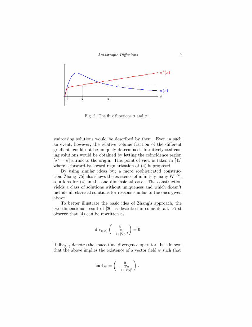
Anisotropic Diffusions 9

sσ(s)

σ∗(s)

s− s s+

Fig. 2. The flux functions σ and σ∗.

staircasing solutions would be described by them. Even in suchan event, however, the relative volume fraction of the differentgradients could not be uniquely determined. Intuitively staircas-ing solutions would be obtained by letting the coincidence region[σ∗ = σ] shrink to the origin. This point of view is taken in [45]where a forward-backward regularization of (4) is proposed.

By using similar ideas but a more sophisticated construc-tion, Zhang [75] also shows the existence of infinitely many W1,∞-solutions for (4) in the one dimensional case. The constructionyields a class of solutions without uniqueness and which doesn’tinclude all classical solutions for reasons similar to the ones givenabove.

To better illustrate the basic idea of Zhang’s approach, thetwo dimensional result of [20] is described in some detail. Firstobserve that (4) can be rewritten as

div(t,x)

(u

− ∇u1+|∇u|2

)= 0

if div(t,x) denotes the space-time divergence operator. It is knownthat the above implies the existence of a vector field ψ such that

curlψ =

(u

− ∇u1+|∇u|2

).

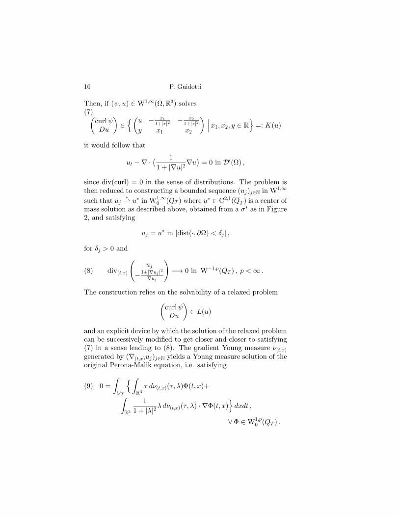
10 P. Guidotti

Then, if (ψ, u) ∈W1,∞(Ω,R3) solves(7)(

curlψDu

)∈(u − x1

1+|x|2 − x21+|x|2

y x1 x2

) ∣∣∣x1, x2, y ∈ R

=: K(u)

it would follow that

ut −∇ ·( 1

1 + |∇u|2∇u)

= 0 in D′(Ω) ,

since div(curl) = 0 in the sense of distributions. The problem isthen reduced to constructing a bounded sequence (uj)j∈N in W1,∞

such that uj∗ u∗ in W1,∞

0 (QT ) where u∗ ∈ C2,1(QT ) is a center ofmass solution as described above, obtained from a σ∗ as in Figure2, and satisfying

uj = u∗ in [dist(·, ∂Ω) < δj ] ,

for δj > 0 and

(8) div(t,x)

(uj

−1+|∇uj |2∇uj

)−→ 0 in W−1,p(QT ) , p <∞ .

The construction relies on the solvability of a relaxed problem(curlψDu

)∈ L(u)

and an explicit device by which the solution of the relaxed problemcan be successively modified to get closer and closer to satisfying(7) in a sense leading to (8). The gradient Young measure ν(t,x)

generated by (∇(t,x)uj)j∈N yields a Young measure solution of theoriginal Perona-Malik equation, i.e. satisfying

(9) 0 =

∫QT

∫R3

τ dν(t,x)(τ, λ)Φ(t, x)+∫R3

1

1 + |λ|2λ dν(t,x)(τ, λ) · ∇Φ(t, x)

dxdt ,

∀ Φ ∈W1,p0 (QT ) .

Anisotropic Diffusions 11

where∫R3

τ dν(t,x)(τ, λ) = ∂tu∗ ,

∫R3

λ dν(t,x)(τ, λ) = ∇u∗ ,

and

∫R3

λ

1 + |λ|2dν(t,x)(τ, λ) = σ∗(∇u∗) .

While the details of the procedure are not given here, it is pointedout that the construction of the center of mass solution requires aninitial datum u0 ∈ C3,1(Ω) and a modified flux function σ∗ derivedfrom the original taking into consideration the value of ‖∇u0‖∞.Again non-uniqueness stems in essence from the arbitrariness ofthe effective flux function σ∗.

§3. Regularizations and Relaxations

3.1. Spatial Regularizations

In [68] Weickert contends that “regularization is modeling”.While undoubtedly interesting from a mathematical point of view,the question of capturing some or all solutions of the Perona-Malikequation through an approximation procedure, is somewhat inconflict with the pragmatic need for viable alternate (image) mod-els. Regularizations and (time-)relaxations of (4) are an importantsource of such alternatives and are therefore of independent inter-est as they essentially rely on their own distinct “edge detectors”.This is an important point as it makes engineering and study-ing the mathematical properties of regularizations a worthwhileinvestigative goal.

Regularization is typically taken to mean the replacement ofthe unknown in an equation’s nonlinear term, in the situation athand 1

1+|∇u|2 , by a more regular version of it. In [17], the authors

propose the use of a Gaussian kernel for the purpose, yielding

(10) ut = ∇ ·( 1

1 + |∇Gσ ∗ u|2∇u).

As the a priori-bound in the L∞-norm (5) remains valid for theregularized equation, one readily obtains that

‖∇Gσ ∗ u‖L∞ ≤ c(σ)‖u‖L∞ ≤ c(σ)‖u0‖L∞ .

12 P. Guidotti

The equation therefore never degenerates and solutions can existglobally as shown in [17]. This approach has the disadvantage ofre-introducing blur into solutions (at least for small scales, ini-tially) and thus blunting the sharpening capabilities of Perona-Malik. This is one of the reasons why alternative, milder reg-ularizations were sought. An important feature of the Perona-Malik equation is that it admits, at least on a purely formal level(as already mentioned when discussing [55]), piecewise constantfunctions (built from characteristic functions of sets with smoothboundaries) as steady-states. This lends some heuristic justifica-tion to the strong sharpening effect of the equation. Any standardregularization such as that of [17] does not preserve this salientand, arguably, essential property of (4). Some authors have at-tempted to overcome this short-coming. Cottet and Germain [25],for instance, looked for a model which would not exhibit trivialdynamical behavior. They implement the idea by considering theregularized reaction-diffusion model

(11) ut = σε2∇ ·(Aε(u)∇u

)+ f(u)

and then deriving a linearized/discrete version of it with the de-sired properties. The matrix Aε is chosen as (essentially) the or-thogonal projection to the direction τε perpendicular to∇uε whereuε is a mollified version of u, i.e. such that

Aε(u)v = (τε · v)τε where τε =1√

|∇uε|2 + ε2

(−∂x2uε∂x1uε

)whereas the reaction term satisfies

f(±1) = 0 , rf(r) > 0 , r ∈ (−1, 1) \ 0 .

Notice that, unlike [17], this regularization does not formally ap-proach (4) in the limit of vanishing ε. It actually converges to adiffusionless limiting equation. The reaction term is indeed essen-tial in their analysis which is limited to special piecewise constantfunctions of the form

u =

−1 , x /∈ D ,

1 , x ∈ D ,

Anisotropic Diffusions 13

forD satisfying some assumptions. This reaction-diffusion is taylor-made to have the above type of piecewise constant functions be-have like almost steady-states and thus generates a non-trivial be-havior of solutions. Their effort to devise a model with this kindof properties underscores the desire to obtain well-posed mod-els with non-trivial dynamics of Perona-Malik type. In a simi-lar vein of truly anistropic diffusions, Weickert in [71] (see also[68, 72, 69, 70]) proposed two models, one which he termed edge-enhancing and one labeled as coherence enhancing. The first moreclosely mimics the Perona-Malik paradigm in that the diffusiontensor D(u) in

ut = ∇ ·(D(u)∇u

)is chosen as to have eigenvectors v1 and v2 satisfying

v1 ‖ ∇uσ and v2 ⊥ ∇uσ ,

and eigenvalues chosen as

λ1 = g(|∇uσ|2) and λ2 = 1 .

While the diffusion so obtained never inverts its direction it stillcan degenerate in direction perpendicular to level sets of u. Inthe second model a measure of local coherence is introduced viathe spectral gap µ1 − µ2 which is obtained from the eigenvalues0 ≤ µ2 ≤ µ1 of Jρ(∇uσ) = Kρ ∗

(∇uσ∇uTσ

), where Kρ serves a

regularizing purpose. The choice of tensor is similar to the above.One takes a diffusion tensor with the same eigenvectors v1 and v2

as Jρ and sets the corresponding eigenvalues to

λ1 = α and λ2 =

α , µ1 = µ2 ,

α+ (1− α)e−c/(µ1−µ2)2m , otherwise

where α ∈ (0, 1).A well-posed model proposed in [47] shows that a strong edge-

enhancing character is not incompatible with spatial regulariza-tion. The idea is to weaken the nonlinear diffusion coefficient inPerona-Malik only very slightly by the use of fractional deriva-tives. The corresponding model reads

(12) ut −∇ ·( 1

1 + |∇1−εu|2∇u)

= 0 .

14 P. Guidotti

The fractional gradient can be defined component-wise in variousways. In [47] the authors choose to work in a periodic settingand to define it through its Fourier symbol in a standard way.Well-posedness (the problem is no longer of forward-backwardtype) is not the only benefit of this model. It actually turns outthat the use of slightly less than one derivative, obtained choos-ing ε ∈ (0, 1/2), allows one to prove that characteristic functionsof smooth sets (or combinations thereof) are stationary solutionsof the equation and greatly influence the dynamic behavior ofthe equation. Numerical experiments show that typical solutionsdo relatively quickly evolve towards a piecewise constant functionin their vicinity and subsequently converge to a trivial steady-state over the long run. Latter convergence is slow and occursthrough gradual decrease in the size of the jumps. Implementa-tions of Perona-Malik show that this indeed happens on a muchlonger time scale than the “simplification” to piecewise constancy.As (12) is locally well-posed, it suppresses the initial phase ofalmost instantaneous singularity formation (onset of staircasing)observed in implementations of Perona-Malik and related to lackof convexity. It does so, however, without preventing singularityformation all together. Analytical results concerning (12) and arelated model are obtained in [44, 46] and [43]. These results aremostly local in time, however, and thus fall short of clarifying theinteresting issue of global existence of smooth or weak solutionsfor the model relating to potential finite time singularity forma-tion, which would help better understand the numerical findings.Known PDE techniques do not seem to apply in this case. Whileit is possible to regularize the equation by adding viscosity andobtain limits for approximating sequences of solutions, it is notclear how to carry the equation to the limit. This is a price paidby the loss of variational structure incurred when introducing thefractional derivative. It is also observed that there is a nice tran-sition from Perona-Malik to classical linear diffusive behavior as εwanders from 0 to 1 as shown in [46] in the one dimensional case.

An even milder regularization was proposed in [45] where thePerona-Malik equation is regularized by a viscous term (δ > 0)

(13) ut −∇ ·([

1

1 + |∇u|2+ δ]∇u

)= 0

Anisotropic Diffusions 15

Even after regularization, the equation remains of forward-backwardtype (at least for δ < 1/8). It is the formal gradient flow of themodified energy functional

(14) PMδ(u) =1

2

∫Ω

[log(1 + |∇u|2) + δ|∇u|2

]dx ,

which, unlike (2), is eventually convex. This regularization pre-serves the time scale of singularity formation but reduces stair-casing (“microstructured” jumping) to a milder micro-structuredramping with alternate gradients of finite size (which depends onδ). Functional (14) has a non-trivial convexification which canbe taken as to uniquely (and naturally) determine a center ofmass solution in a Young-measure type construction of weak so-lutions. While [45] follows a procedure first devised in [31] (seealso [21, 57] for precursors in the elliptic case) in order to con-struct weak Young measure valued solutions of (13), an approachbased on minimizing movements (see [2] or the classical [30, 28])can also be taken to directly construct a center of mass solutionfirst and, only, subsequently generate a Young measure solutionexplicitly by exploiting the specifics of the flux function. While (asin [65, 75, 20]) general Young measure solutions are not unique,those constructed in this fashion are (see [45, 31]). Regulariza-tions of this type were subsequently considered in [48] by usingthe p-Laplacian in place of the Laplacian, i.e., using

Eδ,p(u) =

∫Ω

[12

log(1 + |∇u|2) +δ

p|∇u|p

]dx ,

for p ∈ [1,∞). Gamma convergence techniques allow to identifya time scale such that the vanishing viscosity limit (δ = 0) solu-tions of the associated gradient flows satisfy the Total Variationminimization flow

ut −∇ ·( ∇u|∇u|

)= 0 .

The proof is carried out forp = 2 in [23]. Notice that the re-laxation of the limiting functional for p = 1 does coincide withthe TV functional. From a dynamical point of view, regulariza-tion (13) replaces the staircasing effect of Perona-Malik with what

16 P. Guidotti

Fig. 3. Microstructured gradient for a typical solutionof (13).

could be called a micro-ramping phenomenon by which the effec-tive (center of mass) solution is actually Holder (even Lipschitz)continuous while its gradient exhibits a micro-structure (capturedby a Young-measure) comprised of alternating gradients of smalland large size. See [45] for more detail and Figure 3 for a one di-mensional illustration. Micro-ramping would formally be replacedby stair-casing in the limit of vanishing viscosity on the fast timescale of its occurrence. The slow time scale is indeed captured bythe Gamma limit mentioned above.

Fourth order regularizations have also been considered. In [9]this approach is taken in the one dimensional context. The drivingenergy functional is modified to

(15) EεBF (u) =

1

2

∫ 1

0

[εu2

xx + log(1 + u2x)]dx .

Anisotropic Diffusions 17

The authors of [9] are able to capture the long time behavior ofthe equation (evolution of piecewise constant data) by using Γ-convergence techniques in combination with the appropriate scal-ing. Latter reads ε2 = ν4 log(1 + 1/ν2) and is motivated by anestimate of the energy of a single jump discontinuity which alsoleads to the rescaled energy

EνBF (u) =

EεBF

ν log(1 + 1/ν2).

This family of energies L1-Γ-converges to

EBF (u) = γ∑x∈J(u)

|[u]x|1/2 ,

an energy defined on L1([0, 1]

)which is finite on a subspace of

SBV([0, 1]

)-functions with vanishing absolutely continuous part

of the derivative. The constant γ has to be chosen appropriatelyand [u]x is the jump of u at x ∈ J(u), where J(u) is the not nec-essarily finite jump set of u. They also studied the minimizingmovements evolution engendered by this energy originating in ini-tial data with finitely many and with infinitely many jumps. In thecase of finitely many jumps, the evolution is mostly determinedby a system of ODEs for the jump height with the exception offinitely many “singularization” times at which one or more jumpdiscontinuities disappear (their size vanishes). The location ofdiscontinuities (as long as they are present) is an invariant of theevolution.

3.2. Temporal regularizations/relaxations

The Perona-Malik equation can also be regularized by convo-lution or relaxation in time. The latter approach is proposed inan early image processing paper by [61]. In this paper the authorssuggest to delay or smooth out the effect of the nonlinearity byreplacing (4) by the system

(16)

ut = ∇ ·

(1

1+v2∇u),

vt = ω(ρ ∗ |∇u|2 − v

),

18 P. Guidotti

or the system

(17)

ut = ∇ ·

(1

1+v2∇u),

vt = ω(|∇u|2 − v + σ2

2 ∆u),

In both case some delay (ω−1 > 0) along with some regulariza-tion (ρ and σ > 0) is introduced in an effort to partially tamethe strength of the original nonlinearity. Perona-Malik is recov-ered in the limit as ω → ∞, σ → 0, and ρ → δ, where δ nowdenotes the Dirac distribution. Weickert in [68] cites [63] as a ref-erence that P.L. Lions, in a private communication to Mumford,claimed that (16) is a well-posed regularization of (4). A numberof researcher have taken up the analysis of variations of the abovemodels. Among them one finds [24, 7, 8, 1]. The last paper con-siders a regularization of (4) by time convolution with a positivekernel θ

ut = ∇ ·( 1

1 + θ ∗t |∇u|2∇u),

where θ ∗t |∇u|2(t) =∫ t

0 θ(t− τ)|∇u|2(τ) dτ . This model turns outto be locally well-posed and globally well-posed when the supportof θ is bounded away from zero, so that the nonlinearity does notinclude information up to the present time. It is referred to [1] fora detailed account. However, the rationale put forth by the authorfor considering this time-delayed model is its formal connection toa semi-explicit Euler discretization of the original (4)

un+1 − un

h= ∇ ·

( 1

1 + |∇un|2∇un+1

)where the nonlinearity would be evaluated at the previous timestep. The authors of [24] considered the following relaxation

ut −∇ ·(L∇u) = 0 ,

Lt − L = F (∇Gσ ∗ u) ,

where L is a matrix-valued function representing the diffusion ten-sor connected to the gradient of u by the second equation. If Lis assumed to be initially positive definite, F to be bounded withbounded continuous derivative with nonnegative definite range,

Anisotropic Diffusions 19

and Gσ(for σ > 0) to be a bounded C1-kernel with bounded de-rivative, it is proved in [24] that the system possesses a uniquesolution on any time interval in appropriately chosen functionspaces. Finally in [7, 8] the limiting case where ρ becomes theDirac delta function is considered with the modified relaxationequation

vt = F (|∇u|2)− v ,where F is introduced as a technical device (read regularizingtruncation) to ensure the validity of a priori estimates. Morerecently [64] analyzes the well-posedness of a model of type (17)with relaxation equation given by

vt = λ∆v + (1− λ)(|∇u| − v

).

for a parameter λ ∈ (0, 1) which can be chosen dynamically innumerical implementations.

§4. Semi-discrete models

Regularizations of the type described above have the distinctadvantage of working in any space dimension. This is particu-larly important when it comes to applications to image processingwhere the dimension is typically at least two. In dimension one,however, more detailed analyses can often be performed. In sucha context, an appealing alternative to regularizations of the typedescribed in the previous section is given by spatial discretization.This way the PDE reduces to an ODE system and the mathe-matical problems stemming from concavity of the continuous lim-iting equation can be avoided altogether. Such regularizationsdo, furthermore, mimic numerical schemes used in practical im-plementations of the model and their analysis can shed light onthe observed behavior of such algorithms. Particularly well un-derstood is the long time behavior of (4) which can be capturedby letting the mesh size of the discretization converge to zero byconcurrently speeding up the evolution in order to capture a non-trivial limit in the sense of Γ convergence. This approach is takenin a number of papers concerning the one dimensional case in-cluding [11, 12, 10, 9, 22]. Paper [12] contains a result on theasymptotic expansion (in the sense of Γ-convergence) of the dis-crete Perona-Malik functional and [10] derives a system of ODEs

20 P. Guidotti

connecting jump sizes and locations describing the evolution ofpiecewise constant initial data in a long time limit of the semi-discrete Perona-Malik scheme with Dirichlet boundary conditionswhich reads

(18) ut = D−n( D+

n u

1 + |D+n u|2

).

Here D±n stand for the for forward and backward difference quo-tients of the piecewise constant function u on [0, 1] with a finitenumber of jump discontinuities at the grid points of a uniformgrid of mesh size 1/n for n ∈ N . For convenience the collectionof all such functions is denoted by PCn. For technical reasonssome of the results contained in these two papers do, however,not apply to the precise nonlinearity in (18) nor can they handlethe evolution beyond the first singularization time. Latter is thetime when plateaus of piecewise constancy of the solution mergeremoving one or more discontinuities. Relying on these resultsand making an elegant use the theory of maximal slope curves[30, 29, 2], the authors of [22] obtain a complete description ofthe asymptotic slow time evolution of limiting solutions to (18)with more natural (from the application point of view) Neumannboundary conditions. They are able to obtain a global in timeevolution by renormalizing the driving energy after each singular-ization in the following manner. The discrete Perona-Malik energyfor which (18) can be viewed as a gradient flow is given by

(19) EnPM (u) =

1

2

∫log(1 + |D+

n u|2)dx , u ∈ PCn .

A reinterpretation of an asymptotic expansion of [12] yields

Γ− limn→∞

Gkn(u) =

−∞ , u ∈ PCD , |D| < k ,

Gk∞(u) , u ∈ PCD , |D| = k ,

∞ , otherwise,

where PCD is the space of piecewise constant functions with ex-actly k jumps d ∈ D = d1, . . . , dk of size Jd in the open interval

Anisotropic Diffusions 21

(0, 1) and

Gkn(u) = nEn

PM (u)− k log n , Gk∞(u) =

k∑j=1

log(|Jdj |

)are defined on the space PCn and on the subspace of piecewiseLipschitz and subcritical functions PSD, i.e. satisfying the sub-criticality inequality |D+u(x)| < 1 on their regularity subintervalsand having jumps located at exactly k points collected in the setD. The functionals Gk

n lead, up to the renormalization term, toan accelerated version of the gradient flow associated to (19) withacceleration factor given by the number of grid points. The renor-malization term k log n is important but inconsequential as far asthe associated gradient system on PCn

ut = −n∇PMn(u) = −∇Gnk(u) , for t > 0 ,

is concerned. All function spaces used can be thought of as sub-spaces of L2(0, 1) and the all functionals are thought of as beingdefined on the latter, extending the original by the value ∞ ifnecessary. Then, in essence, it is possible to describe the limitingevolution of initial data in PCD via the limiting system of ODEsgiven by

(20)

a′0(t) = 1

d1−d01

a1(t)−a0(t) , a0(0) = a00

a′i(t) = 1di+1−di

[1

ai+1−ai −1

ai−ai−1

], ai(0) = a0i

a′k(t) = − 1dk+1−dk

1ak−ak−1

, ak(0) = a0k ,

where i = 1, . . . , k−1, the initial datum u0 takes values a0i on theinterval (di, di+1) for i = 0, . . . , k, and d0 := 0 as well as dk+1 := 1.It is recalled that di ∈ (0, 1) for i = 1, . . . , k. System (20) hasto be interpreted as to evolve initial data with no jump trivially(constant in time) and piecewise constant ones with exactly kjumps by the given equations up to the first singularization timewhere the number of jumps has necessarily to decrease (otherwisethe solution could be continued a little longer). It then evolvesthe newly created piecewise constant functions according to (20)with a different k reflecting the new number of jumps. This evo-lution is well-defined as it can be shown that solutions are Holder

22 P. Guidotti

continuous up to the singularization time. See [22] for a detailedaccount.

An alternative approach to taking the vanishing mesh sizelimit on a mesh dependent time scale was taken in [35]. Insteadof speeding up the evolution by rescaling time, the author choosesthe threshold parameter κ of

ut =( 1

1 + u2x/κ

ux)x

as a function of the mesh size h (of a uniform grid on [0, 1]). Therelation leading to a distinguished non-trivial limit for the evolu-tion of piecewise smooth initial data with discontinuities at a finitenumber of points is given by κ(h) = h−1, in which case nonlinearboundary conditions are obtained in the limiting problem acrossthe discontinuity points and linear diffusion away from these. Ifui denotes the solution on the interval [dj , dj+1) for j = 0, . . . , nwhere d1, . . . , dn−1 are the jump locations, d0 and dn are the endpoints of the unit interval, and

Ji = ui+1(di, t)− ui(di, t)

is the jump at di for i = 1, . . . , n − 1, then the limiting problemcan be formulated as

(21)

∂tui = ∆ui , in (di−1, di) , for t > 0 ,

∂xui(di) = ∂xui+1(di) = 1Ji, for i = 1, . . . , n− 1 ,

∂xui(di) = 0 , for i = 0, n .

The idea of choosing a mesh size dependent parameter to obtainan interesting limit was already present in [18] where it was usedin a stationary context for the Mumford-Shah functional (1). Asrescaling κ is at least formally akin to rescaling time, the limit-ing system also qualitatively captures the medium and long timebehavior of solutions to numerical experiments with diffusive be-havior away from the discontinuities and jump height reductionat the discontinuities. As in [22], a Holder continuity argumentallows the author of [35] to continue solutions beyond singulariza-tion times when one or more jumps vanish. For a detailed analysisit is referred to the original paper. Finally in [36] a (partial) two-dimensional comparison principle (other than the one of [54]) is

Anisotropic Diffusions 23

obtained. Latter is subsequently applied in order to derive aninteresting stability property of the (one dimensional) numericalscheme for (4) which shows that small enough “random” pertur-bations to initial data are quickly reabsorbed during the evolution,in agreement with numerical observations.

§5. A Hybrid Model

Since the ill-posedness and instability of Perona-Malik in itscontinuous formulation manifests itself in the onset of an un-controlled number of jumps (captured qualitatively by Young-measure valued solutions discussed earlier), another approach canbe taken which avoids this issue completely by preventing the un-stable region to loose thickness in the limit. This is done in [56]where the author proposes a new image model by which the jumpset is given and fixed but jump size is allowed to evolve. Moreprecisely let u : Ω→ R be an image which is slowly varying awayfrom an edge set Γ (in fact a finite union of Lipschitz curves).Then u is evolved from its inital value I by the gradient flow ofthe functional(22)

EK(u) =

∫Ω\Γ

[G(|∇u|) +

1

2α(u− I)2 dx+ h

∫ΓF (∣∣[u]Γ

∣∣/h) dσΓ

so that it is smoothed out away from Γ and the size of its jumpsis reduced over time. The nonlinear terms are chosen so that Gbehaves like F in the subcritical region and becomes quadraticat infinity, whereas F is of Perona-Malik type. The parameter hmeasures the edge “thickness”. It is referred to the original articlefor a comprehensive description and for the rationale behind thischoice. Assuming that G−λ| · |2 and F +µ| · |2 are convex for somechoice of λ, µ ∈ [0,∞), nonlinear semigroup theory ([14]) can beapplied to obtain an exponentially growing semigroup and, thus,a unique solution to the evolutionary inclusion problem

∂tu+ ∂EK(u) 3 0 in t > 0 ,

on L2(Ω). As the assumptions suggest, the result is obtained byshifting the generator to ∂EK(u) + 2βu and treating ∂EK(u) as a

24 P. Guidotti

Lipschitz perturbation of the shifted operator. The resulting semi-group is therefore exponentially growing in general. Thus Perona-Malik’s instability has been effectively tamed but only mildly, asexponential divergence of nearby initial data over the long runshows. This model, like the one proposed in [47], has the benefitof delivering a well-posed model which predicts and agrees withnumerical observations. Unlike the latter, however, it requiresthat the discontinuity set be known and fixed in advance.

§6. Fourth Order Models

Finally it should be mentioned that, while the mathemati-cal community focussed on obtaining satisfactory insight into thePerona-Malik model and its many modifications, the more appliedor application oriented community followed, among other avenuesthe trail of fourth order models. The motivation was almost al-ways to try and prevent the cartoonish look generated by secondorder methods due to their strong tendency to produce piecewiseconstant output. Without any claim of completeness, here is alist of references to modeling papers [66, 67, 73, 58, 33, 32, 4, 51,52, 49] where higher order models are considered and another,[13, 42, 34, 50], of papers dealing with related mathematical ques-tions. Mathematical results are much more scarce for higher ordermethods than for their second order counterpart and many impor-tant basic questions remain open.

§7. A Final Remark

PDE based methods in image processing are only one of a vari-ety of techniques employed in practice. While they often enjoy theadvantage of allowing for a geometric interpretation and a cleantheoretical analysis, they typically lead to slower numerical im-plementations. Therefore statistical and/or wavelet-based meth-ods are often preferred (see [15] and references therein). These,however, fall far outside the scope of this paper, which aimed atpresenting an overview of the research activities of the past twentyyears engendered by the Perona-Malik model only.

Anisotropic Diffusions 25

References

[ 1 ] H. Amann. Time-Delayed Perona-Malik Problems. Acta Math.Univ. Comenianae, LXXVI:15–38, 2007.

[ 2 ] L. Ambrosio, N. Gigli, and G. Savare. Gradient Flows in MetricSpaces of Probability Measures. Lecture in Mathematics. ETHZurich. Birkhauser Verlag, Basel-Boston-Berlin, 2008.

[ 3 ] L. Ambrosio and V.M. Tortorelli. Approximation of functionalsdepending on jumps by elliptic functionals via Γ- convergence.Comm. Pure Appl. Math., 43:999–1036, 1990.

[ 4 ] Jian. Bai and X.-C. Feng. Fractional Order Anisotropic Diffusionfor Image Denoising. IEEE Transactions on Image Processing,16(10):2492–2502, 2007.

[ 5 ] J.D. Ball and R.D. James. Fine phase mixtures as minimizers ofenergy. Arch. Rational Mech. Anal., 100:13–52, 1987.

[ 6 ] J.D. Ball and R.D. James. Proposed experimental tests of a theoryif fine microstructures and the two-well problem. Phil. Royal Soc.Lon., 338A:389–450, 1992.

[ 7 ] A. Belahmidi. Equations aux derivees partielles appliquees a larestoration et a l’agrandissement des images. Ph.D. Thesis. Uni-versite Paris-Dauphine, Paris, 2003.

[ 8 ] A. Belahmidi and A. Chambolle. Time-delay regularization ofanisotropic diffusion and image processing. M2AN Math. Model.Numer. Anal., 39(2):231–251, 2005.

[ 9 ] A. Bellettini and G. Fusco. The Γ-limit and the related gradientflow for singular perturbation functionals of Perona-Malik type.Trans. Amer. Math. Soc., 360(9):4929–4987, 2008.

[10] G. Bellettini, M. Novaga, and M. Paolini. Convergence for long-times of a semidiscrete Perona-Malik Equation in one dimension.Math. Models Methods Appl. Sci., 21(2):1–25, 2011.

[11] G. Bellettini, M. Novaga, M. Paolini, and C. Tornese. Convergenceof discrete schemes for the Perona-Malik equation. J. DifferentialEqs., 245(4):892–924, 2008.

[12] G. Bellettini, M. Novaga, M. Paolini, and C. Tornese. Classificationof the Equilibria for the semi-discrete Perona-Malik Equation.Calcolo, 46(4):221–243, 2009.

[13] A. Bertozzi and J. Greer. Low-Curvature Image Simplifiers: GlobalRegularity of Smooth Solutions and Laplacian Limiting Schemes.Communications on Pure and Applied Mathematics, LVII:0764–0790, 2004.

26 P. Guidotti

[14] H. Brezis. Operateurs Maximaux Monotones et Semi-Groups deContractions dans les Espaces de Hilbert. Nort-Holland, Ams-terdam, 1973.

[15] A. Buades, B. Coll, and J.M. Morel. A Review of Image DenoisingAlgorithms, with a New One. Multiscale Modeling and Simula-tions, 4(2):490–530, 2005.

[16] J. Canny. Finding Edges and lines in images, volume 720 of TechReport. Artificial Intelligence Laboratory, MIT, 1983.

[17] F. Catte, P.-L. Lions, J.-M. Morel, and T. Coll. Image selectivesmoothing and edge-detection by non-linear diffusion. SIAM J.Numer. Anal., 29(1):182–193, 1992.

[18] A. Chambolle. Image segmentation by variational methods: Mum-ford and shah functional and the discrete approximations. SIAMJ. Appl. Math., 55(3):827–863, 1995.

[19] T. F. Chan and L. Vese. Active contours without edges. IEEE Tans.Image Processing, 10:266–277, 2001.

[20] Y. Chen and K. Zhang. Young Measures Solutions of the Two-Dimensional Perona-Malik Equation of Image Processing. Comm.Pure and Appl. Math., 5(3):617–637, 2006.

[21] M. Chipot and D. Kinderlehrer. Equilibrium Configurations ofCrystals. Arch. Rational Mech. Anal., 103(3):237–277, 1988.

[22] M. Colombo and M. Gobbino. Slow time behavior of the semidis-crete Perona-Malik scheme in one dimension. SIAM J. math.Anal., 43(6):2564–2600, 2011.

[23] M. Colombo and M. Gobbino. Passing to the limit in maximal slopecurves: from a regularized Perona-Malik equation to the totalvariation flow. Math. Models Methods Appl. Sci., 22(8):125001719 pp., 2012.

[24] G.-H. Cottet and M. El Ayyadi. A volterra type model for imageprocessing. IEEE Trans. Image Processing, 7:292–303, 1998.

[25] G.-H. Cottet and L. Germain. Image Processing through ReactionCombined with Nonlinear Diffusion. Mathematics of Computa-tion, 61(204):659–673, 1993.

[26] B. Dacorogna. Weak continuity and weak lower semicontinuity ofnonlinear functionals, volume 922 of Lecture Notes in Math.Springer, Berlin, 1982.

[27] B. Dacorogna and I. Fonseca. A-B-quasiconvexity and implicit par-tial differential equations. Calc. Var. PDEs, 14:115–149, 2002.

[28] E. de Giorgi. New problems on minimizing movements. In BoundaryValue Problems for PDE and Applications, volume 29 of RMARes. Notes Appl. Math., pages 81–98. Masson, Paris, 1993.

Anisotropic Diffusions 27

[29] E. de Giorgi. Evolution problems in metric spaces and steepest de-scent curves. In L. Ambrosio, G. Dal Maso, M. Forti, and S. Spag-nolo, editors, Ennio de Giorgi. Selected Papers, volume Ennio deGiorgi, Selected Papers, pages 527–533. Springer Verlag, Berlin,2006.

[30] E. de Giorgi, A. Marino, and M. Tosques. Problemi di evoluzionein spazi metrici e curve di massima pendenza. Atti Accad. Naz.Lincei Rend. Cl. Sci. Fis. Mat. Natur., 68(8):180–187, 1980.

[31] S. Demoulini. Young Measure Solutions for a Nonlinear ParabolicEquation of Forward-Backward Type. SIAM J. math. Anal.,27:376–403, 1996.

[32] S. Didas, B. Burgeth, A. Imiya, and J. Weickert. Regularity andScale-Space Properties of Fractional High Order Linear Filter-ing. In Scale Space and PDE Methods in Computer Vision,volume 3459 of Lecture Notes in Computer Science. SpringerBerlin/Heidelberg, 2005.

[33] S. Didas, J. Weickert, and B. Burgeth. Stability and local FeatureEnhancement of Higher Order Nonlinear Diffusion Filtering. Pat-tern Recognition, 3663:451–458, 2005.

[34] S. Didas, J. Weickert, and B. Burgeth. Properties of higher ordernonlinear diffusion filtering. J. Math. Imaging Vision, 35(3):208–226, 2009.

[35] S. Esedoglu. An analysis of the perona-malik scheme. Comm. PureAppl. Math., 54:1442–1487, 2001.

[36] S. Esedoglu. Stability Properties of the Perona-Malik Scheme.SIAM J. Numer. Anal., 44:1297–1313, 2006.

[37] M. Ghisi and M. Gobbino. Gradient Estimates for the Perona-MalikEquation. Math. Ann., 3:557–590, 2007.

[38] M. Ghisi and M. Gobbino. A Class of Local Classical Solutionsof Perona-Malik. Trans. Amer. Math. Soc., 361(12):6429–6446,2009.

[39] M. Ghisi and M. Gobbino. An example of global classical solutionfor the Perona-Malik equation. Comm. PDEs, 36(8):1318–1352,2011.

[40] M. Ghisi and M. Gobbino. On the evolution of subcritical regions forthe Perona-Malik equation. Interfaces Free Bound., 13(1):105–125, 2011.

[41] M. Gobbino. Entire Solutions of the one-dimensional Perona-MalikEquation. Comm. Partial Differential Equations, 32(4–6):719–743, 2007.

28 P. Guidotti

[42] J. B. Greer and A. L. Bertozzi. Traveling wave solutions of fourthorder PDEs for image processing. SIAM J. Math. Anal., 36(1):38–68 (electronic), 2004.

[43] P. Guidotti. A new Nonlocal Nonlinear Diffusion of Image Process-ing. Journal of Differential Equations, 246(12):4731–4742, 2009.

[44] P. Guidotti. A New Well-posed Nonlinear Nonlocal Diffusion. Non-linear Analysis Series A: Theory, Methods, and Applications,72:4625–4637, 2010.

[45] P. Guidotti. A backward-forward regularization of the Perona-Malikequation. Journal of Differential Equations, 252(4):3226–3244,2012.

[46] P. Guidotti. A family of nonlinear diffusions connecting Perona-Malik to standard diffusion. Discrete and Continuous DynamicalSystems - Series S, 5(3), 2012.

[47] P. Guidotti and J. Lambers. Two New Nonlinear Nonlocal Diffu-sions for Noise Reduction. Journal of Mathematical Imaging andVision, 33(1):25–37, 2009.

[48] P. Guidotti, J. lambers, and Y. Kim. Image restoration with a newclass of forward-backward-forward diffusion equations of Perona-Malik type with Applications to Satellite Image Enhancement.Under review.

[49] P. Guidotti and K. Longo. Two Enhanced Fourth Order DiffusionModels for Image Denoising. Journal of Mathematical Imagingand Vision, 40(2):188–198, 2011.

[50] P. Guidotti and K. Longo. Well-Posedness for a Class of Fourth Or-der Diffusions for Image Processing. Nonlinear Differential Equa-tions and Applications, Online first:1–19, 2011.

[51] M.R. Hajiaboli. A Self-governing Hybrid Model for Noise Removal.In Advances in Image and Video Technology, volume 5414 ofLecture Notes in Computer Science. Springer Berlin/Heidelberg,2008.

[52] M.R. Hajiaboli. An Anisotropic Fourth-Order Partial DifferentialEquation for Noise Removal. In Scale Space and VariationalMethods in Computer Vision, volume 5567 of Lecture Notes inComputer Science. Springer Berlin/Heidelberg, 2009.

[53] B. Kawohl. Variational versus PDE-based approaches in mathemat-ical image processing. In Singularities in PDE and the Calculusof Variations, volume 44 of CRM Proc. Lecture Notes, pages 113–126. AMS, Providence, RI, 2008.

[54] B. Kawohl and N. Kutev. Maximum and comparison principle forone-dimensional anisotropic diffusion. Math. Ann., 311(1):107–123, 1998.

Anisotropic Diffusions 29

[55] S. Kichenassamy. The Perona-Malik paradox. SIAM J. Appl. Math.,57(5):1328–1342, 1997.

[56] S. Kichenassamy. The Perona-Malik Method as an Edge PruningAlgorithm. J. Math. Imaging Vis., 30:209–219, 2008.

[57] D. Kinderlehrer and P. Pedregal. Weak convergence of integrandsand the young measure representation. SIAM J. Math. Anal.,23(1):1–19, 1992.

[58] M. Lysaker, A. Lundervold, and X.C. Tai. Noise Removal UsingFourth Order Differential Equations with Applications to MedicalMagnetic Resonance Images in Space-Time. IEEE Transactionon Image Processing, 12(12):1579–1590, 2003.

[59] D. Marr and E. Hildreth. Theory of edge detection. Proc. Roy. Soc.London, 207:187–217, 1980.

[60] D. Mumford and J. Shah. Optimal Approximation by piecewisesmooth functions and associated variational problems. Comm.Pure Appl. Math., 42:577–685, 1989.

[61] M. Nitzberg and T. Shiota. Nonlinear image filtering with edge andcorner enhancement. IEEE Trans. Pattern Anal. and MachineIntelligence, 14:826–833, 1992.

[62] P. Perona and J. Malik. Scale-space and edge detection usinganisotropic diffusion. IEEE Transactions Pattern Anal. MachineIntelligence, 12:161–192, 1990.

[63] P. Perona, T. Shiota, and J. Malik. Anisotropic Diffusion. In B.M.ter Haar Romeny, editor, Geometry-driven diffusion in computervision, pages 72–92. Kluwer, Dordrecht, 1994.

[64] V.B. Surya Prasath and D. Vorotnikov. On a System ofAdaptive Coupled PDEs for Image Restoration. To ap-pear in Journal of Mathematical Imaging and Vision.http://www.springerlink.com/content/1g3735618t454811/fulltext.pdf.

[65] S. Taheri, Q. Tang, and K. Zhang. Young measure solutions and in-stability of the one-dimensional Perona-Malik equation. J. Math.Anal. Appl., 308:467–490, 2005.

[66] J. Tumblin and G. Turk. LCIS: A boundary hierarchy for detail-preserving contrast reduction. In Proceedings of the SIGGRAPH1999 Annual Conference on Computer Graphics, August 8-13,1999, Los Angeles, CA, USA, Siggraph Annual Conference Se-ries, pages 83–90. ACM Siggraph, Addison-Wesley, Longman,1999.

[67] G. Wei. Generalized Perona-Malik equation for image restoration.IEEE Signal Processing Letters, 6(7):165–167, 1999.

30 P. Guidotti

[68] J. Weickert. A Review of Nonlinear Diffusion Filtering. In Scale-Space Theory in Computer Vision, number 1252 in Lecture Notesin Computer Science, pages 3–28. Springer, Berlin, 1997.

[69] J. Weickert. Coherence-enhancing diffusion filtering. InternationalJournal of Computer Vision, 31:111–127, 1999.

[70] J. Weickert. Coherence-enhancing diffusion of colour images. Imageand Vision Computing, 17:201–212, 1999.

[71] Joachim Weickert. Anisotropic Diffusion in Image Processing.Ph.D. Thesis. Universitat Kaiserslautern, Kaiserlautern, 1996.

[72] Joachim Weickert. Anisotropic Diffusion in Image Processing.ECMI Series. Teubner Verlag, Stuttgart, 1998.

[73] Y.L. You and M. Kaveh. Fourth order partial differential equa-tions for noise removal. IEEE Transaction on Image Processing,9(10):1723–1730, 2000.

[74] K. Zhang. On the structure of quasi-convex hulls. Ann. Inst. H.Poincare Anal. Non Lineaire, 15:663–686, 1998.

[75] K. Zhang. Existence of infinitely many solutions for the one-dimensional Perona-Malik model. Calc. Var., 26(2):171–199,2006.

Department of Mathematics340 Rowland HallIrvine, CA 92697, USAE-mail address: gpatrick@math.uci.edu