ANISOTROPIC MATERIAL MODELING AND IMPACT

SIMULATION OF A BRUSH CUTTER CASING MADE OF

A SHORT FIBER REINFORCED PLASTIC

Oskar Norman

Master Thesis LIU-IEI-TEK-A--14/01935--SE

Department of Management and Engineering

Division of Solid Mechanics

ANISOTROPIC MATERIAL MODELING AND IMPACT

SIMULATION OF A BRUSH CUTTER CASING MADE OF

A SHORT FIBER REINFORCED PLASTIC

Supervisor at LiU: Larsgunnar Nilsson

Supervisor at Dynamore Nordic AB: Mats Landervik

Oskar Norman

Master Thesis LIU-IEI-TEK-A--YY/XXXXX--SE

Department of Management and Engineering

Division of Solid Mechanics

i

Abstract

A popular way to reduce weight in industrial products without compromising the strength or stiffness is to

replace components made of metal by plastics that have been reinforced by glass fibers. When fibers are

introduced in a plastic, the resulting composite usually becomes anisotropic, which makes it much more complex

to work with in simulation software. This thesis looks at modeling of such a composite using the multi-scale

material modeling tool Digimat.

An injection molding simulation of a brush cutter casing made of a short fiber reinforced plastic has been

performed in order to obtain information about the glass fiber orientations, and thus the anisotropy, in each

material point. That information has then been transferred over from the injection mesh to the structural mesh

via a mapping routine. An elasto-viscoplastic material model with failure has been employed and calibrated

against experimental data to find the corresponding material parameters. Lastly, a finite element analysis

simulating a drop test has been performed. The results from the analysis have been compared with a physical

drop test in order to evaluate the accuracy of the methodology used. The outcome has been discussed,

conclusions have been drawn and suggestions for further studies have been presented.

ii

Preface

This master thesis has been carried out during the spring semester of 2014 as the final stage of the Mechanical

Engineering program at the division of Solid Mechanics at Linköping University, Linköping, Sweden. The work has

been done at Dynamore Nordic AB in Linköping and Husqvarna in Huskvarna was an industrial partner for the

project. Dr. Mats Landervik was the supervisor from Dynamore Nordic AB and Prof. Larsgunnar Nilsson was the

supervisor from Linköping University.

Acknowledgements

I would like to thank Dynamore Nordic AB for giving me the opportunity to carry out this interesting project. A

special gratitude goes to my supervisor Dr. Mats Landervik for all the advice during the thesis. Furthermore, I

would like to thank Mikael Palm at Husqvarna for great cooperation, e-Xstream for support on Digimat issues

and DSM for the experimental data and answering questions regarding the material modeling. Last but not least,

I want to thank Prof. Larsgunnar Nilsson, who was my supervisor from Linköping University, for all expertise.

iii

Abbreviations

AR Aspect ratio

CAD Computer aided design

CPU

EP

EVP

Central processing unit

Elasto-plastic

Elasto-viscoplastic

FE

FI

Finite element

Failure indicator

MFH

PA

Mean-field homogenization

Polyamide

QS

RE

Quasistatic

Reverse engineering

RH Relative humidity

RVE Representative volume element

SFRP Short fiber reinforced plastics

iv

TABLE OF CONTENTS

1 Introduction .................................................................................................................................................... 1

1.1 Background ............................................................................................................................................ 1

1.2 Objectives .............................................................................................................................................. 1

1.3 Prerequisites and limitations ................................................................................................................. 2

1.4 Work flow .............................................................................................................................................. 2

2 Theory ............................................................................................................................................................ 4

2.1 Composite materials .............................................................................................................................. 4

2.2 Homogenization .................................................................................................................................... 5

2.3 Injection molding ................................................................................................................................... 6

2.4 Fiber orientations .................................................................................................................................. 7

2.5 Elasto-viscoplasticity .............................................................................................................................. 8

2.6 Failure criteria ...................................................................................................................................... 10

3 Method ......................................................................................................................................................... 12

3.1 FE meshes ............................................................................................................................................ 12

3.1.1 Injection FE mesh ............................................................................................................................ 12

3.1.2 Structural FE mesh .......................................................................................................................... 13

3.2 Moldex3D ............................................................................................................................................ 14

3.3 Digimat ................................................................................................................................................ 15

3.3.1 Digimat-MAP ................................................................................................................................... 15

3.3.2 Digimat-MX ..................................................................................................................................... 16

3.3.3 Digimat-CAE..................................................................................................................................... 19

3.4 LS-DYNA ............................................................................................................................................... 19

3.5 LS-PrePost ............................................................................................................................................ 21

4 Results .......................................................................................................................................................... 22

4.1 Moldex3D ............................................................................................................................................ 22

4.2 Digimat ................................................................................................................................................ 24

4.2.1 Digimat-MAP ................................................................................................................................... 24

4.2.2 Digimat-MX ..................................................................................................................................... 26

4.2.3 Digimat-CAE..................................................................................................................................... 27

4.3 LS-DYNA ............................................................................................................................................... 28

4.4 LS-PrePost ............................................................................................................................................ 28

5 Discussion ..................................................................................................................................................... 32

6 Conclusions ................................................................................................................................................... 33

7 Suggestions for further studies .................................................................................................................... 34

8 List of Figures ................................................................................................................................................ 35

v

9 List of Tables ................................................................................................................................................. 36

10 References .................................................................................................................................................... 37

11 Appendix ...................................................................................................................................................... 38

1

1 INTRODUCTION

Fiber reinforced plastics are becoming more and more popular in industrial applications due to their light weight

and relatively low cost compared to other engineering materials such as steel and aluminum. The purpose of

reinforcing a plastic with fibers is to make the material stronger without compromising its density significantly.

Besides increasing the strength of the material, this procedure also increases the complexity of its

microstructure. As soon as fibers are introduced in a plastic, the material will usually no longer be isotropic with

identical material properties in all directions, but anisotropic with different material properties in different

directions.

Research in the field of composite materials started about 50 years ago and was a high focus area of for the

coming decades, and it still is today. One of the most challenging parts in the development of the mechanics for

fiber reinforced composites has been to find models to characterize failure (Christensen, 2005). In later years,

lots of resources have been put into the study of failure behavior since it has shown to be one of the most

important aspects in the field.

To obtain fair results when performing finite element (FE) analyses with fiber reinforced plastics, the amount of

work and computational cost will increase compared to analyses of isotropic materials. Since the material

properties depend on the fiber orientations, which themselves depend on how the component is being

manufactured, it is not a trivial task to implement this information into FE simulations. However, it is today

possible to use software to simulate the manufacturing process in order to predict fiber orientations and thence

obtain the corresponding material properties to be used in the structural analysis.

1.1 BACKGROUND

In this thesis work, a brush cutter casing made of a short fiber reinforced plastic (SFRP) is studied. The material

is Akulon® K224-PG6, a polyamide 6 (also known as nylon 6) reinforced with short glass fibers (about 0.1 - 1 mm

long) accounting for 30 % of the composite’s mass. The casing is protecting the actuating device and is located

on the top of the brush cutter. It is being manufactured using injection molding, which is a very common

technique for producing SFRP parts.

The product concerned for this project is a Husqvarna 545RXT, which is especially made for professional use and

already exists on the market. Husqvarna is a major player in the gardening machines sector and has many years

of experience when it comes to structural FE simulations. Though, as of writing, Husqvarna is not taking the

anisotropy into account in a satisfying manner when running structural analyses with SFRP parts, but they want

to be able to do so. Digimat is a material modeling tool that can be used for this exact purpose, but before

Husqvarna decides to start using Digimat it is desirable to understand how the implementation works, see if the

results are desirable and get a hint of the work load trade-off.

Both an injection molding simulation will be performed as well as an implementation of this new information

into a structural impact simulation to simulate a drop test.

1.2 OBJECTIVES

The main objectives of this thesis are to

• Understand the methodology and work flow of a project of this kind, from the injection molding

simulation to the results of the impact simulation

• Implement a new material model with fiber orientations taken into account in an already existing impact

simulation model

• Investigate the influence of anisotropy in the material model

• Compare the simulation results with physical test results

2

1.3 PREREQUISITES AND LIMITATIONS

A few parts are not to be developed or performed during this thesis work and are provided or performed by

other parts. Those parts are listed below

• FE meshes are provided by Husqvarna

• Experimental data for the material is provided by DSM

• Injection parameters are provided by Euroform

• The impact simulation model is provided by Husqvarna

• Suggestion of a new design is not an objective, but findings that might lead to improvements, in terms

of failure resistance, will be presented

1.4 WORK FLOW

The software products that will be used during the project are

1. Moldex3D® (CoreTech System Co., Ltd., 2013) – Injection molding simulation

2. Digimat® (e-Xstream engineering, 2013) – Mapping and material modeling

3. LS-DYNA® (Livermore Software Technology Corporation, 2012) – Impact simulation

4. LS-PrePost® (Livermore Software Technology Corporation, 2014) – Post processing of simulation results

A picture describing the work flow, including input data required and output data obtained for each step, is

presented in the end of this section, Figure 1.

Without taking the anisotropy into account, a natural work flow would be to follow the same steps as presented

in Figure 1, but to exclude the two first steps (injection molding simulation in Moldex3D and material modeling

in Digimat) and start with the impact simulation right away, provided that necessary material parameters are

known.

The tool that is used to simulate the injection molding process is Moldex3D, primarily because Husqvarna already

uses it and it has support for outputting the fiber orientations to the material modeling tool Digimat. It is also

one of the most advanced injection molding simulation tools on the market. The output from Moldex3D is a fiber

orientation file, corresponding to the injection FE mesh, containing one fiber orientation tensor for each

integration point.

Before the material modeling can take place, the fiber orientations have to be mapped to the structural FE mesh

that is to be used in the impact simulation. This is a task that requires the injection FE mesh, the corresponding

fiber orientation file and the structural FE mesh. The output is a mapped fiber orientation file, related to the

structural FE mesh, containing one fiber orientation tensor for each integration point.

To create an accurate material model in Digimat, some necessary material parameters must be known and others

have to be determined. The data that has to be known in this case are both the density of the plastic as well as

material parameters for the isotropic and elastic glass fiber inclusions, i.e. density, Young’s modulus, Poisson’s

ratio and the ratio between the length and diameter of the fibers, hereinafter referred to as the aspect ratio

(AR). The data that has to be determined by reverse engineering (RE) in this case is material parameters for the

matrix material necessary to fit the material model, e.g. Young’s modulus, Poisson’s ratio, yield stress, hardening

parameters and viscoplasticity parameters. The output from the material modeling part is a calibrated material

model to be implemented in the FE simulation.

There is usually a step of preprocessing before the FE simulation can take place, e.g. FE meshing, setting up the

model, defining simulation parameters, set initial conditions and define contacts. As mentioned, that has already

been done by Husqvarna, so the coupled Digimat/LS-DYNA explicit analysis to simulate a drop test does not

require too much setup in this work. The coupled analysis works in such a way that at each time step LS-DYNA

3

computes the macroscopic strains and communicates with Digimat to receive the corresponding material

properties in every integration point throughout the FE mesh. The coupled Digimat/LS-DYNA analysis will

henceforth in the report be called the LS-DYNA analysis for simplicity and to avoid confusion.

LS-PrePost is used to post process the results, to evaluate them and to draw conclusions from them. Physical

drop tests have been performed for the simulations to be compared with. The evaluation of the simulation

results will mainly consist of visual comparison with pictures from the physical drop test, both because that is

the main interest and because no accelerometer data or other measurements are available.

FIGURE 1 - DESCRIPTION OF THE WORK FLOW WITH INPUTS AND OUTPUTS

4

2 THEORY

In this chapter, some of the theory behind all concerned parts in the thesis will be briefly presented. It is written

in such a way that most fundamentals related to materials and finite elements are omitted, but details specific

for the subject are included. In cases where details however are omitted there will most often be a proposed

source for further explanation for the interested reader.

2.1 COMPOSITE MATERIALS

The SFRP in this case consists of one matrix material and one phase of inclusions. The matrix material is a

polyamide (PA) and the inclusions are glass fibers. The challenge when performing FE analyses with composite

materials is to predict the interaction between the microstructure and the macroscopic properties. To fully

perform analyses and solve the problems on the scale of the microstructure would be very computationally

demanding. Therefore it is suitable to distinguish between two scales; the microscopic scale, where the material

it treated as heterogeneous, and the macroscopic scale, where the material is treated as locally homogeneous.

In Digimat, the connection between the two scales rely on the principle of so-called representative volume

elements (RVE). Each RVE corresponds to a material point on the macroscopic scale, and has to be large enough

to represent the heterogeneity but small compared to the solid body. The approach in Digimat to allow for

transitions between the two scales is summarized in (e-Xstream engineering, 2013).

FIGURE 2 - THE CONCEPT OF TRANSITION BETWEEN SCALES

In order to find constitutive relations of quantities on the different scales, continuum mechanics are applied on

the macroscopic scale. Assume that for each macroscopic material coordinate � the macroscopic strain���� is

known and the objective is to compute the macroscopic stress����. The average quantity over an RVE is defined

by

⟨���, �⟩ � 1�� ���, ��

�� (2.1)

where is the position of a micro particle in a local frame of the RVE, � is the domain and � the volume of the

RVE. Integration is performed in the micro coordinates where ���, � is the micro field inside the RVE. With use

of this relation, it has been proven, for instance by (Toll, 2005), that the average strain and stress in an RVE are

equal to the macroscopic strain and stress respectively. Consequently,

Microscopic scale Macroscopic scale

RVE

5

⟨�⟩ = � (2.2)

⟨�⟩ = � (2.3)

The objective in the end is to find the macroscopic stresses for given macroscopic strains in each material point.

2.2 HOMOGENIZATION

A widely used approach in order to predict the influence of the microstructure on the overall properties is to

apply a homogenization technique. The aim is to find an equivalent homogeneous material with the same

effective stiffness as the initial heterogeneous composite, subjected to the same boundary conditions. The

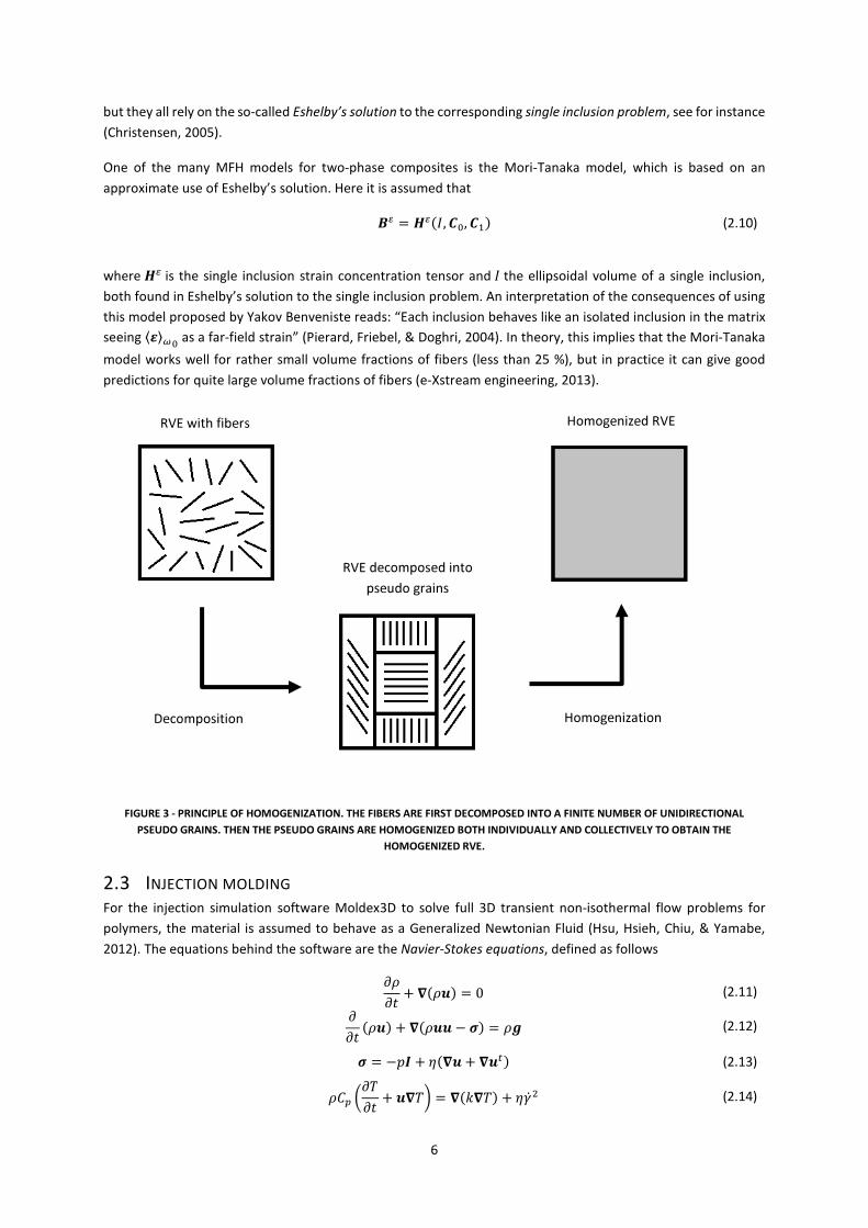
principle of homogenization is presented in Figure 3.

There are several homogenization techniques for different problems, all with their own advantages and

disadvantages. In this thesis work, the so-called mean-field homogenization (MFH) model to approximate the

volume averages will be used, both because it is supported in Digimat and because it is very CPU cost-effective

(Pierard, Friebel, & Doghri, 2004). It is important to know that MFH does not solve the stress and strain fields on

the full microscopic level, but on a homogenized version of it.

Assume a two-phase composite with a matrix material reinforced with fibers that are identical in terms of shape,

orientation and material properties. Using the so-called rule of mixtures, the volume averages of the strain and

stress fields over the full domain � of the RVE can be written as

� = ��⟨�⟩��+ ��⟨�⟩��

(2.4)

� = ��⟨�⟩��

+ ��⟨�⟩�� (2.5)

where subscripts 0 and 1 indicate the matrix and fiber phase respectively and � is the volume fraction of each

phase such that �� + �� = 1. But as mentioned earlier, strains and stresses for each phase will not be evaluated,

hence at this point it is convenient to make use of so-called strain concentration tensors, and the problem can

be rewritten on the following form

⟨�⟩��= ��: ⟨�⟩��

(2.6)

⟨�⟩��

= ��: � (2.7)

As can be concluded by Equations (2.6) and (2.7) above, the two tensors �� and �� are not independent. By

using Equations (2.4), (2.6) and (2.7), the relation between the two strain concentration tensors can be written

as

�� = ��: ���� + 1 − ���� �� (2.8)

where � is the fourth-order identity tensor. With help of the relations above, the macroscopic stiffness can then

be written on its final form

� = ����:�� + 1 − ����� : ���� + 1 − ���� �� (2.9)

where the volume fraction �� as well as the stiffness for each phase �� and �� are assumed to be known entities.

Hence, the final step in order to solve this equation, is to find an expression for the strain concentration

tensor��. This is where the many MFH models differ, as they are based on different assumptions and conditions,

6

but they all rely on the so-called Eshelby’s solution to the corresponding single inclusion problem, see for instance

(Christensen, 2005).

One of the many MFH models for two-phase composites is the Mori-Tanaka model, which is based on an

approximate use of Eshelby’s solution. Here it is assumed that

�� = ���,��,��� (2.10)

where �� is the single inclusion strain concentration tensor and � the ellipsoidal volume of a single inclusion,

both found in Eshelby’s solution to the single inclusion problem. An interpretation of the consequences of using

this model proposed by Yakov Benveniste reads: “Each inclusion behaves like an isolated inclusion in the matrix

seeing ⟨�⟩�� as a far-field strain” (Pierard, Friebel, & Doghri, 2004). In theory, this implies that the Mori-Tanaka

model works well for rather small volume fractions of fibers (less than 25 %), but in practice it can give good

predictions for quite large volume fractions of fibers (e-Xstream engineering, 2013).

FIGURE 3 - PRINCIPLE OF HOMOGENIZATION. THE FIBERS ARE FIRST DECOMPOSED INTO A FINITE NUMBER OF UNIDIRECTIONAL

PSEUDO GRAINS. THEN THE PSEUDO GRAINS ARE HOMOGENIZED BOTH INDIVIDUALLY AND COLLECTIVELY TO OBTAIN THE

HOMOGENIZED RVE.

2.3 INJECTION MOLDING

For the injection simulation software Moldex3D to solve full 3D transient non-isothermal flow problems for

polymers, the material is assumed to behave as a Generalized Newtonian Fluid (Hsu, Hsieh, Chiu, & Yamabe,

2012). The equations behind the software are the Navier-Stokes equations, defined as follows

���� + ���� = 0 (2.11)

��� ��� + ����− �� = �� (2.12)

� = −�� + ���+ ���� (2.13)

��� ����� + ���� = ����� + �� � (2.14)

Decomposition Homogenization

RVE with fibers

RVE decomposed into

pseudo grains

Homogenized RVE

7

where � is the density, � the time, � the velocity vector, � the full stress tensor, � the pressure, � the

gravitational vector, � the second-order identity tensor, � the viscosity, �� the specific heat, � the temperature,

� the thermal conductivity and �� the equivalent shear rate.

2.4 FIBER ORIENTATIONS

Fiber orientations in fiber reinforced plastics is a key component to determine the material properties and its

behavior when subjected to loads. It is quite complex to describe the fiber orientation distribution in a

component, but its nature highly depends on the material’s flow properties. Two different kinds of flows can be

identified to describe the fiber orientation through the thickness in a component. The first one is the shear flow,

which usually occurs close to the boundaries of the component, and the second one is the extensional flow,

which usually occurs close to the core in a component. Together, these two flow types form the so-called skin-

core effect (Bernasconi, Cosmi, & Dreossi, 2008). The skin-core effect induces fibers that are subjected to shear

flow to be highly aligned in the melt flow direction and fibers that are subjected to extensional flow to be highly

oriented across the melt flow direction, see Figure 4 below for a picture illustrating the phenomenon.

FIGURE 4 - THE SKIN-CORE EFFECT VISUALIZED IN AN INJECTION MOLDED PLATE1

To describe the fiber orientation mathematically, it is efficient to utilize the tensor notation. A second-order

orientation tensor, describing the orientation distribution in each material point, can be written as

� � ��� ����� (2.15)

where � is the orientation unit vector and ��� is the orientation density function, i.e. the probability of finding

a fiber with the orientation� at this specific material point. Since � is symmetric, 6 components are enough to

describe the tensor

� � !"�� "�� "��"�� "��"��# (2.16)

1 The picture is taken from www.ides.com with permission granted from IDES.

8

where the diagonal components !��, !�� and ! describe the intensity of the fiber orientation in the 1:st, 2:nd

and 3:rd direction, respectively. The non-diagonal terms are slightly more complex to picture and a curious

reader is thus recommended to read (e-Xstream engineering, 2013) for a more thorough explanation.

The orientation tensor has the following characteristics

• The diagonal terms ! (no summation) must all have values between 0 and 1, 0 ≤ ! ≤ 1

• The sum of the diagonal terms must be equal to 1, tr"� = ! = 1

• The absolute value of the non-diagonal terms must be less or equal to 0.5, #!�# ≤ 0.5

• If the non-diagonal terms are 0, then the 1:st, 2:nd and 3:rd direction coincide with the principal

directions

A few examples for special cases of orientation tensors and how to interpret them is shown below

• " = $ 1 0 0

0 0

0

% represents the case where all fibers in the material point are fully aligned in the 1:st

principal direction (notice that !�� ≥ !�� ≥ !)

• " = $1/2 0 0

1/2 0

0

% represents the case where fibers are randomly aligned in the 2D-plane described

by the 1:st and 2:nd principal directions

• " = &1/3 0 0

1/3 0

1/3

' represents the case of full random 3D fiber orientation

The orientation change, with respect to time, can be expressed as (index notation is used here for simplicity)

(!�(� = )*�!�� − !�*��+ + ,)-�!�� + !�-�� − 2-� !�� + + 2��� ).� − 3!�+ (2.17)

where *� are the components of the vorticity or spin tensor, , = /0� − 1�//0� + 1�a shape factor, which

is a function of the fiber AR, -� are the components of the rate of deformation tensor, !�� are the components

of the fourth-order orientation tensor, �� ∈ 0, 1 the interaction coefficient (to account for fiber-fiber

interaction) and .� the Kronecker delta. To solve this equation, the fourth-order orientation tensor !�� has to

be approximated using a so-called closure approximation method. The method primarily used in Moldex3D is the

hybrid closure approximation, which is further explained in (Han & Ima, 1999).

2.5 ELASTO-VISCOPLASTICITY

Elasto-viscoplasticity (EVP) is a model of a material’s behavior that distinguishes the fully elastic region and the

plastic region. Furthermore, the plastic part is strain rate dependent, hence the term viscoplasticity. Since

Digimat is the software to be used for the material modeling, all equations, formulas and models are derived

from (e-Xstream engineering, 2013).

The total strain can be written as the sum of the elastic strain and the plastic strain

� = �� + �� (2.18)

For the elastic part, the stress-strain relation can be written as

� = �: �� (2.19)

9

where � is Hooke´s operator, which for orthotropic materials and with the use of Voigt notation utilized by

Digimat can be written as

� =

1222223��� ��� �� 0 0 0��� �� 0 0 0� 0 0 0��� 0 0456. ��� 0���78

88889 (2.20)

where its inverse, the so-called compliance matrix, reads

: =

12222222222223

1;� −<��;�

−<�;

0 0 0

−<��;� 1;�

−<�;

0 0 0

−<�;� −

<�;�

1;

0 0 0

1=�

0 0

456.1=�

0

1=��

78888888888889

(2.21)

where ; is the Young’s modulus along axis > , <� is the Poisson’s ratio for a contraction in direction ? when

subjected to extension in direction > and =� is the shear modulus in direction ? whose normal coincide with

direction >. For symmetry reasons, <�/; = <�/;� (no summation), which means that 9 independent material

coefficients have to be determined in order to find the full compliance (or stiffness) matrix.

In Digimat, the plasticity is modeled by the so called @�-plasticity model, based on the equivalent according to

von Mises

A�� = B3@� = CA�� − A���� + A�� − A�� + A − A���� + 6A��� + A�� + A�� �2

(2.22)

The limit that separates the elastic and the plastic parts is the initial yield stress A� , giving the elasticity the

following condition to satisfy

A�� ≤ A� (2.23)

Consequently, for the plastic part, when the condition is no longer fulfilled, the approach is slightly different. As

the stress-strain relation becomes non-linear and plastic deformation takes place, it is possible to express the

equivalent stress as

A�� = A� + 0�� (2.24)

10

where 0�� is the hardening stress and � is the accumulated plastic strain. There exist different models to

calculate the hardening stress and one of the more advanced supported by Digimat is the Exponential and linear

law, which can be written as

0�� = �� + 0�1 − D���� (2.25)

where � is a linear hardening modulus, 0� a hardening modulus and 6 a hardening exponent.

Furthermore, the accumulated plastic strain is defined by

��� = E � F�(F�

�

(2.26)

where � is the accumulated plastic strain rate defined by

� = �23G �: G ���/� (2.27)

where G � is the plastic strain rate.

A yield function is defined by

HA,0� = A�� − A�� = A�� − A� − 0�� ≤ 0 (2.28)

which indicates that the material is still in the elastic region if the condition is fulfilled, but evolves to the plastic

region if not. The plastic strain rate is given by the normality rule

G � = � �H�A (2.29)

Several models exist to account for the viscoplastic effect in terms of high strain rate sensitivity. One of them is

the so-called Hyperbolic sine law, also known as the Prandtl law. This model is one of the three that are supported

by Digimat and is defined as

� = A�� �sinh �HI���

(2.30)

where � and I are viscoplastic coefficients and 6 is a viscoplastic exponent.

2.6 FAILURE CRITERIA

Failure criteria are used to predict the point of breakage for a material that is subjected to loads. One of the

models to predict failure is the so-called Tsai-Hill 3D Transversely Isotropic strain based criterion, defined as

H� = Bℱ�G� (2.31)

ℱ�G� = G��G�� − G�� − G� + G��G − 4G��J�

+G�� − G�� + 16G��K�

+4G��� + G�� �L�

(2.32)

11

where �� is the failure indicator (FI), $� the failure function, % is the maximum axial tensile strain, & the

maximum in-plane tensile strain and ' the maximum transverse shear strain (e-Xstream engineering, 2013). The

criterion is met when �� reaches or exceeds the value of 1.

As can be concluded by its name, Tsai-Hill 3D Transversely Isotropic assumes the material to be isotropic in the

23-plane, where the 11-direction represents the first principal direction of the fiber orientations, see Figure 5

below for an interpretation of the conditions explained.

FIGURE 5 - CONCEPT FOR DEFINING THE PLANE FOR TRANSVERSAL ISOTROPY

This failure model also assumes identical failure conditions for tension and compression. For the material failure

surface to form a closed envelope, the parameters % and & must satisfy the relation& ( 2%.

12

3 METHOD

In this chapter, each analysis is described and how each software is used is explained. For an overview of the

work flow, see Figure 1 in section 1.4.

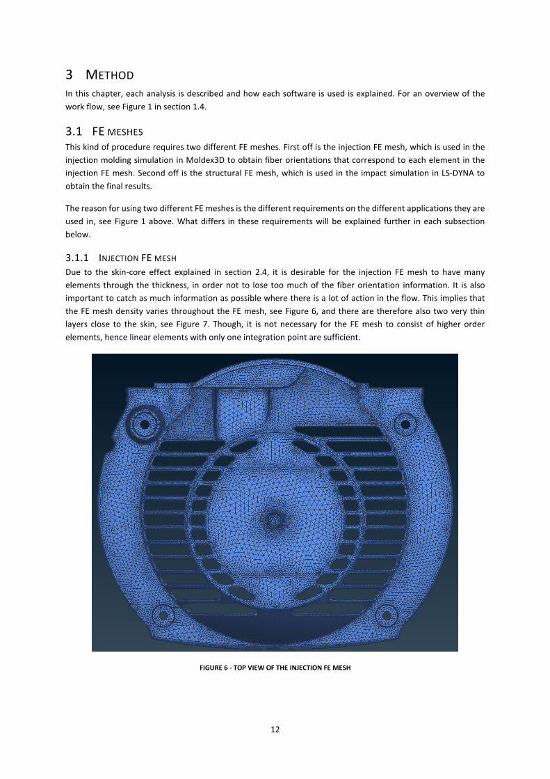
3.1 FE MESHES

This kind of procedure requires two different FE meshes. First off is the injection FE mesh, which is used in the

injection molding simulation in Moldex3D to obtain fiber orientations that correspond to each element in the

injection FE mesh. Second off is the structural FE mesh, which is used in the impact simulation in LS-DYNA to

obtain the final results.

The reason for using two different FE meshes is the different requirements on the different applications they are

used in, see Figure 1 above. What differs in these requirements will be explained further in each subsection

below.

3.1.1 INJECTION FE MESH

Due to the skin-core effect explained in section 2.4, it is desirable for the injection FE mesh to have many

elements through the thickness, in order not to lose too much of the fiber orientation information. It is also

important to catch as much information as possible where there is a lot of action in the flow. This implies that

the FE mesh density varies throughout the FE mesh, see Figure 6, and there are therefore also two very thin

layers close to the skin, see Figure 7. Though, it is not necessary for the FE mesh to consist of higher order

elements, hence linear elements with only one integration point are sufficient.

FIGURE 6 - TOP VIEW OF THE INJECTION FE MESH

13

FIGURE 7 - CROSS-SECTIONAL VIEW OF THE INJECTION FE MESH

3.1.2 STRUCTURAL FE MESH

When performing explicit FE simulations it is desirable to have a uniform structural FE mesh, meaning that the

elements throughout the FE mesh should be as equal in size as possible, see Figure 8 and Figure 9. The reason is

that the time step, which is computed by the FE solver, is based on the smallest element size in the FE mesh using

the formula

���� = M�N� (3.1)

where M� is a characteristic length of the smallest element and N� the speed of sound through the material of the

element, which can be calculated from

N� = C ;�1 − <���� (3.2)

For the structural load case, an FE mesh with linear 4-noded tetrahedron solid elements will be used. Also, the

element formulation will be of LS-DYNA type 13, which is a formulation for single integration point tetrahedron

elements. It is a constant stress element with nodal pressure averaging and is recommended for materials with

a Poisson’s ratio greater than 0. These were the best available options related to the structural FE mesh due to

Digimat’s rather limited support for element types and formulations.

14

FIGURE 8 - TOP VIEW OF THE STRUCTURAL FE MESH

FIGURE 9 - CROSS-SECTIONAL VIEW OF THE STRUCTURAL FE MESH

3.2 MOLDEX3D

For the injection simulation in Moldex3D to be performed, a number of inputs are required. The injection FE

mesh is imported into Moldex3D, but also the system for the injection molding process has to be designed. All

required components, such as gates, runners and cooling channels, were in this case included in the injection FE

mesh mold base created by Husqvarna.

Input data, in terms of material and injection parameters, has to be set in Moldex3D. The material used, Akulon®

K224-PG6, exists in Moldex3D’s material database and material parameters are thereby automatically set. The

filling time, which is considered a primary input, is taken from the manufacturer’s record. The remaining

15

parameters, such as pressure and temperature, are suggested by Moldex3D itself based on both the filling time

and the material choice.

The output that is generated from the injection molding simulation is a fiber orientation file corresponding to

the injection FE mesh. Other outputs, such as a visualization of the flow, pressure vs. time diagrams, plot of the

temperature fields and weld lines, are also generated by Moldex3D. Even though some of these outputs are not

intended to serve as input for any future step, it gives a good hint if the simulation is realistic or not as well as

some insight of the procedure.

3.3 DIGIMAT

The material model is created in the multi-scale material modeling tool Digimat. The software has many

capabilities and can be used in many ways, such as designing new materials or calibrate materials through

experimental data, depending on the user’s needs. In this thesis work it will serve as a mapping and material

modeling tool where the modules, Digimat-MAP, Digimat-MX and Digimat-CAE will be used. For this reason, the

description of the work in Digimat is divided into three parts, one for each module.

3.3.1 DIGIMAT-MAP

Digimat-MAP is used to map information from the injection frame over to the structural frame. In this case only

the fiber orientations are mapped, but it can also be things like, initial stresses, initial temperatures and weld

lines.

Since the fiber orientations obtained in the injection simulation is related to the elements in the injection FE

mesh, a mapping to the structural FE mesh is performed in order to take them into account for the future impact

simulation. For this to be possible, the required inputs to Digimat-MAP are the injection FE mesh (in Digimat

called “Donor mesh”), the corresponding fiber orientation file and the structural FE mesh (in Digimat called

“Receiving mesh”).

When the aforementioned information is imported into Digimat-MAP, some parameters must be specified

before the mapping process can take place. First off is the mapping method option. The mapping method choice

in this case is the so-called Integration point / Node to Integration point method, which transfers fiber orientation

values at integration points or nodes in the injection FE mesh to integration points in the structural FE mesh. This

method is recommended by the software’s developers and gives the best results (see (e-Xstream engineering,

2013) for descriptions of all available methods).

The mapping tolerance, a measure of how far outside the injection FE mesh the integration points of the

structural FE mesh are allowed to be, must be specified, see Figure 10. If the default mapping tolerance, based

on the mean element size in the injection FE mesh, is used and the mapping procedure fails, it gives the user an

idea of where the two FE meshes differ and a chance to refine the structural FE mesh if needed. In this case, a

default mapping tolerance is approximately 0.14, but it is too tight in order to perform the mapping successfully.

A sufficient mapping tolerance of can be found by trial-and-error and is in this case 0.22. The higher mapping

tolerance of 0.22 is preferred over refining the structural FE mesh.

16

FIGURE 10 - PRINCIPLE OF MAPPING TOLERANCE

When the mapping procedure is completed, Digimat computes the mapping error. This is a feature that helps

the user to see the loss in precision after having transferred information between the different FE meshes and

to decide whether the results are sufficient or not.

Outputs, consisting of the fiber orientation file corresponding to the structural FE mesh and graphs showing the

mapping error, are stored for future steps.

3.3.2 DIGIMAT-MX

Digimat-MX is a database tool to store material and experimental data for different materials. A material supplier

can share data with its customers, both material data and ready to run material models that have been generated

through RE, i.e. by calibrating a model against experiments to identify material parameters. RE utilizes an

optimization algorithm in order to minimize the difference between the model results and the experimental data.

To model the material response and obtain the required material parameters, a number of experiments were

performed by DSM and the related results were provided. The tensile specimens that were used in the tests were

cut out from an injection molded plate at three different angles (0°, 45° and 90°) relative to the melt flow

direction (see Figure 11 for a description). They were dried to almost 0 % RH and kept at 23°C during the tests.

The very low humidity in the material makes it more brittle than under normal conditions, say 50 % RH.

FIGURE 11 - INJECTION MOLDED PLATE WITH TENSILE SPECIMEN CUT OUT AT DIFFERENT ANGLES RELATIVE TO THE MELT FLOW

DIRECTION

Element in the

injection FE mesh

Tolerance

17

Table 1 below shows a summary of the different experiments that are used in the material modeling.

TABLE 1 - EXPERIMENTAL DATA USED FOR MATERIAL MODELING

Experiment Loading angle [°] Strain rate [s-1] Temperature [°C] RH [%]

1 0 QS2 23 0

2 45 QS 23 0

3 90 QS 23 0

4 0 1 23 0

5 90 1 23 0

6 0 10 23 0

7 90 10 23 0

8 0 100 23 0

9 90 100 23 0

To visualize the experimental data, two different plots are created, Figure 12 and Figure 13.

FIGURE 12 - GRAPH SHOWING THE THREE QUASISTATIC EXPERIMENTS

2 Quasistatic experiments focus on using a strain rate low enough to avoid strain rate dependent effects, usually

around 0.001 s-1

Tru

e s

tre

ss

True strain

Akulon® K224-PG6

0 deg, QS

45 deg, QS

90 deg, QS

18

FIGURE 13 - GRAPH SHOWING EXPERIMENTS AT ALL DIFFERENT STRAIN RATES

From the characteristics of the graphs in Figure 12 and Figure 13, it is decided to model the material with an

elasto-viscoplastic material model, omitting strain rate dependency in the elastic region. Some small viscoelastic

behavior is however identified in the graphs, but since Digimat does not support any viscoelastic-viscoplastic

material model for the hybrid solution that is going to be utilized in the next step, the elasto-viscoplastic material

model is the best choice available.

A reference microstructure must be defined, in this case based on an average orientation tensor of the inclusion

phase. This information can be determined either by looking at a cross section of the material in a microscope or

by simulating the injection of the molded plate used for the experiments. Since neither of these operations are

performed, an estimation based on common values for an injection molded plate, with some necessary trial and

error tuning, is made. A final average orientation tensor, giving the best fitting results, is found to be

! = $0.72 0 0

0.26 0

0.02

% (3.3)

The parameters that are required to be found for the PA6 matrix material in order to fit the EVP model are the

Young’s modulus, the Poisson’s ratio, the Yield stress, three hardening coefficients and three strain rate

sensitivity coefficients. In order to find them, RE is utilized with an optimization algorithm in Digimat from the

DAKOTA software toolkit. All models and parameters to model the material response are explained in the theory

part in section 2.5.

First, the elasto-plastic (EP) parameters are found based on the three QS experiments and the viscoplastic effect

is then added to find the remaining parameters. However, due to the small viscoelastic effects (see Figure 13) it

is not possible to get good matches for both the QS experiments and the one with higher strain rates

simultaneously. Hence, priority is put onto finding the better match for the experiments with the higher strain

rates, as these are expected to be dominant in the model during the impact.

Tru

e s

tre

ss

True strain

Akulon® K224-PG6

0 deg, 1 s⁻¹

0 deg, 10 s⁻¹

0 deg, 100 s⁻¹

90 deg, 1 s⁻¹

90 deg, 10 s⁻¹

90 deg, 100 s⁻¹

0 deg, QS

90 deg, QS

19

The final part is to find FI based on the experiments. Tsai-Hill 3D Transversely Isotropic (explained in section 2.6)

is used making the design variables the maximum axial tensile strain, the maximum in-plane tensile strain and

the maximum transverse shear strain. Since the experimental data shows no strain rate dependency for failure

(see graph Figure 13), the three QS experiments are sufficient to identify the FI.

3.3.3 DIGIMAT-CAE

Digimat-CAE is a tool used to prepare input data for the FE analysis. The user also has the possibility to choose a

Digimat solution procedure, set integrations parameters, specify the fiber orientation file, etc. Digimat-CAE offers

three different solution procedures, the micro method, the macro method and the hybrid method.

The micro method uses strong multiscale coupling techniques to interactively compute the material properties

at each time step in the FE simulation, and is hence a relatively expensive method in terms of CPU cost. The

macro method completely pre-computes the macroscopic material properties which are kept constant

throughout the complete FE simulation. This means that the method is not suitable for materials with non-linear

behavior, though it is rather fast. The hybrid method is somewhat a compromise of the two methods just

described. It uses weak multiscale coupling techniques but pre-computes the macroscopic material properties

for the Digimat-CAE interface to communicate with the FE simulation at each time step. The hybrid method is

claimed to offer an expected CPU speed-up factor of 20 compared to the micro method, with the limitation that

the user cannot obtain output on the microscopic scale (e-Xstream engineering, 2013).

In this case, non-linear material behavior is expected, a low CPU cost is desirable and the material response on

the microscopic level is of no interest. Hence, the hybrid solution procedure is chosen.

3.4 LS-DYNA

A coupled Digimat and LS-DYNA Explicit analysis is used as FE solver for the impact simulation. Together with the

hybrid solution chosen in the previous step, this procedure lets the FE solver acquire pre-computed material

properties from Digimat at each time step throughout the complete simulation.

As the model for the impact simulation is already setup by Husqvarna, this part does not require much work in

order to be ready to run in LS-DYNA.

A picture of the model, in its upside-down position, ready to drop from 400 mm, is shown in Figure 14, where

the investigated part is the dark blue cover in the bottom part of the picture.

20

FIGURE 14 - SIDE VIEW OF THE FULL SIMULATION MODEL

Notice that the model consists only of the most important parts for the drop test and does not look much like a

full brush cutter. This is because parts that are assumed to have low influence on the results of the simulation

have been replaced with mass and inertia to simplify it and decrease the CPU cost.

To avoid redundant simulation time, the uninteresting part of the drop, i.e. before the model hits the ground,

has been replaced with an equivalent initial velocity. This velocity can be calculated via the energy equilibrium

as

6Oℎ =6��

2⇔ � = B2Oℎ ≈ 2.86/4 (3.4)

The equivalent time it would take for the model to fall 400 mm can be calculated by

ℎ = ℎ� + ��� + O��2

⇔ Pℎ� = 0�� = 0Q ⇔ � = C2ℎO ≈ 28664 (3.5)

and since it is enough to simulate only 3 milliseconds, due to the very short course of event, this replacement

saves a lot of time and unnecessary computation.

Furthermore, what can be seen in Figure 14 is that the screws in the four holes are missing. Instead, all nodes

that would be in contact with a screw are constrained to the red rigid crank-case as extra nodes.

A cross section of the model shows what happens inside it during the impact, Figure 15. The red screw-head in

the middle of the picture is modeled with a rigid constraint relative to the dark blue casing that is studied. Hence,

all loads that will be put onto it will be transferred to the casing, which is the main reason why there is a

compression dominance in it.

21

FIGURE 15 - CROSS-SECTIONAL VIEW OF THE FULL SIMULATION MODEL

3.5 LS-PREPOST

LS-PrePost is the post processing tool used to visualize the outcome of the impact simulation from the previous

step. The post processor makes it possible to obtain results such as plots and graphs of most entities of interest.

22

4 RESULTS

In this chapter, results from all analyses are presented and discussed in sequential order.

4.1 MOLDEX3D

Moldex3D generates a plot called melt front time. Since it is difficult to visualize the flow in a report, only the

final state of the simulation is shown, see Figure 16. Just like the legend is showing, blue color indicates material

that has been inside the mold for a long time compared to the red color which indicates material that has been

injected more recently. This is the top view of the component and the gate is placed in the middle of it, as can

be seen in Figure 17.

FIGURE 16 - FILLED CAVITY FROM THE INJECTION MOLDING SIMULATION IN MOLDEX3D

More importantly, the fiber orientations can be displayed and exported as an *.o2d file, a format supported by

Digimat. Moldex3D is able to visualize the fiber orientation distribution which displays the first, and thus the

largest, eigenvalue, see Figure 17. Recall from the theory, section 2.4, that a large first eigenvalue implies a high

amount of fibers aligned in this direction, whereas a smaller first eigenvalue, 1/3 being the smallest possible,

implies a more random like distribution.

23

FIGURE 17 - FIRST EIGENVALUE OF THE FIBER ORIENTATION TENSOR FOR EACH ELEMENT

Some statistics regarding the first eigenvalue of the fiber orientation distribution can also be generated, see

Figure 18. The graph shows that almost all variations of orientation distributions are represented in the model.

,

FIGURE 18 - STATISTICS REGARDING THE FIRST EIGENVALUE OF THE FIBER ORIENTATION TENSOR

24

4.2 DIGIMAT

4.2.1 DIGIMAT-MAP

As soon as both the injection FE mesh and the corresponding fiber orientation file are imported in Digimat-MAP,

it is possible to visualize the fiber orientations in the software. This visualization should of course represent the

exact same picture as from Moldex3D above, Figure 19. Among the many different display options that are

available, the first eigenvector plot gives the best overview summarized in a single picture.

FIGURE 19 - FIRST EIGENVALUE FOR THE INJECTION FE MESH IN DIGIMAT-MAP

After the mapping onto the structural FE mesh is done, the result can be visualized by the same type of picture.

FIGURE 20 - FIRST EIGENVALUE FOR THE STRUCTURAL FE MESH IN DIGIMAT-MAP

The FE mesh density of the two meshes in Figure 19 and Figure 20 are very different. Recall from Figure 6, Figure

7, Figure 8 and Figure 9 in section 3.1 that the injection FE mesh has rather big elements in some areas and rather

small elements in other areas, whereas the structural FE mesh is more uniform. Because of this, the fiber intensity

25

(the number of colored arrows in the plots) is scaled to make the pictures look more similar. So, instead of

comparing the pictures above, which both can be difficult and misleading, Digimat is able to compute the global

error for each of the six directions in order to give the user an idea of the mapping quality.

FIGURE 21 - GLOBAL ERROR INDICATORS CALCULATED IN ALL DIRECTIONS

As mentioned in section 2.4, a11, a22 and a33 (here corresponding to the global coordinate axes x, y and z) in

Figure 21 are the more intuitive directions and are therefore easier to study. The bars represent the relative

number of elements that contain a specific fiber orientation, for instance, the very first bar pair on the top left

graph shows that elements with a a11 value is between 0 and 0.1 is about 6 % in the injection FE mesh and 1 %

in the structural FE mesh. A perfect mapping without any loss in accuracy would thus result in all bar pairs being

of identical height.

At first sight, the mapping quality looks fairly low. In general, for all graphs, the deviation between the two FE

meshes is biggest for big and small ! (no summation). This phenomenon can be traced back to the differences

in FE mesh structure (recall Figure 6, Figure 7, Figure 8 and Figure 9) and especially the difference through the

thickness with the injection FE mesh having two thin layers of elements close to the skin. The injection FE mesh

therefore catches the skin-core effect well, whereas the structural FE mesh does not have enough elements

through the thickness for the effect to be transferred. A picture confirming this theory is presented in Figure 22.

26

FIGURE 22 - TENSOR COMPONENTS THROUGH THE THICKNESS OF AN INJECTION MOLDED PLATE, AS AN EXPLANATION OF THE SKIN-

CORE EFFECT3

To improve the mapping quality, either the injection FE mesh can be modified to have a structure closer to the

structural FE mesh, or the structural mesh can be modified with a higher FE mesh density and/or using elements

with multiple integration points. In the first case, the skin-core effect will not be caught as good, which gives a

loss in precision even before the mapping step. In the second case, increasing the FE mesh density will affect the

CPU cost negatively and using multiple integration points is not supported by Digimat. Hence, neither of the

options are utilized, and the mapping quality is considered sufficient.

4.2.2 DIGIMAT-MX

After the optimization algorithm has converged, the material model is stored in the database to be used together

with Digimat-CAE in the next step. Results obtained are plotted in graphs showing both the experiments (dashed

lines) and the fitted model (continuous lines) for the QS case, the high strain rate case and FI.

The first fit is the EP material model, which is calibrated against the QS experiments, presented in Figure 23.

FIGURE 23 - CALIBRATION OF AN EP MATERIAL MODEL AGAINST THE QUASISTATIC EXPERIMENTS

3 The picture is taken from “Fiber Contents Effect on the Fiber Orientation in Injection Molded GF/PP Composite

Plates” published in “Proceedings of the SPE Annual Technical Conference 2002 in San Francisco” with permission

granted by the author.

27

As explained in section 3.3.2, the small viscoelastic effects that are identified has in this case to be omitted in the

material modeling, due to missing support of such a model in Digimat with the hybrid solution. Therefore, the

Young’s modulus from the EP fit has to be increased in order for the material model to better fit the high strain

rate experiments. This lead to a worse fit for the QS case, which can be seen in Figure 23 above, but is a decision

based on the fact that high strain rates are expected to be dominant in the impact simulation model.

The viscoplastic effect is then added to the material model and the results can be seen in Figure 24.

FIGURE 24 - CALIBRATION OF AN EVP MATERIAL MODEL AGAINST THE HIGH STRAIN RATE EXPERIMENTS

The last part from the material modeling is to obtain the FI, Figure 25.

FIGURE 25 - CAILBRATION OF FAILURE INDICATORS AGAINST THE QUASISTATIC EXPERIMENTS

The 0° and 90° curves are almost perfectly fitted, whereas the 45° is a rather bad fit. Even though the FI are found

through optimization, it is not always easy to obtain a better fit.

4.2.3 DIGIMAT-CAE

The material model, created in the previous step, is then imported in Digimat-CAE, which pre-computes the

hybrid parameters and two output files are generated. The first one is a material parameter file containing all

28

the material and hybrid parameters to be used for the communication between Digimat and LS-DYNA. The

second one is a material keyword file on the required LS-DYNA format which is implemented in the full model

keyword file for the FE solver to recognize that a Digimat material model is going to be used.

4.3 LS-DYNA

The final results from the impact simulation in LS-DYNA are post processed and visualized in LS-PrePost, which is

presented in the next section.

4.4 LS-PREPOST

To be sure that the impact is fully completed, the velocity of the model is plotted as a function of time, see Figure

26.

FIGURE 26 - VELOCITY IN THE VERTICAL DOWNWARDS DIRECTION OF THE SIMULATION MODEL

The plot above shows that the model falls freely the first 0.4 ms, the impact happens between 0.4 – 2.85 ms, and

then it finally begins to travel upwards, in the opposite direction, for the remaining 0.15 ms. This implies that the

impact is fully completed and that the analysis should include everything of interest.

At the very end of the simulation the results are visualized. The final state of the component is presented in

Figure 27.

-0.5

0.0

0.5

1.0

1.5

2.0

2.5

3.0

0.0 0.5 1.0 1.5 2.0 2.5 3.0

Z-v

elo

city

[m

/s]

Time [ms]

Z-velocity

29

FIGURE 27 - TOP VIEW OF THE CASING AFTER THE FULL IMPACT

As can be seen in the picture, only the component of interest is studied, and therefore the other components

are blanked out. Cracks on the front view can be identified in primarily 9 different regions. To be able to make

comparisons with the physical drop tests, a picture of the same component when dropped from 400 mm is

presented in Figure 28.

30

FIGURE 28 - TOP VIEW OF THE CASING FROM A PHYSICAL DROP TEST FROM 400 MM

When comparing the two pictures, it is obvious that none of the cracks in the model fully coincides with the

physical test. Cracks in regions 4, 7 and 8 in the model are relatively close though, whereas cracks in regions 1,

2, 3, 5, 6 and 9 of the model do not even exist in the physical component.

If the results instead are compared with a physical drop test from a height of 500 mm, Figure 29, some interesting

findings are identified.

31

FIGURE 29 - TOP VIEW OF THE CASING FROM A PHYSICAL DROP TEST FROM 500 MM

Another three cracks occur in this case and two of them, in regions 5 and 6, are more or less correctly predicted

in the simulation model. The third crack is rather close to region 2, but does not coincide with what the model

predicts.

A discussion of the possible reasons behind the deviations is given in the next section.

32

5 DISCUSSION

Crack propagation of the simulation model was predicted, but compared to the physical drop test, the results

are not very accurate. Some elements fail prematurely and there are even cracks in regions without any damage

in the physical test. A few of the reasons why this occurs are known and others can only be speculations.

Regardless, they are discussed separately in this section.

The first issue is related to the element type and element formulation that had to be used in the structural FE

mesh, 4-noded tetrahedron solid elements with element formulation of LS-DYNA type 13. A quadratic 10-noded

solid tetrahedron element with four or five integration points would give much more accurate behavior than an

element with less nodes and only one integration point. Not only would the FE results be more accurate, but also

would more fiber orientation information be utilized and thus give an improved mapping quality, since there is

one fiber orientation tensor related to each integration point. Unfortunately, the used Digimat version does not

support elements with multiple integration points.

The second problem is the limits of the hybrid solution in Digimat not allowing for failure models that distinguish

between failure caused by tension and compression. Since the casing is subjected to an impact when hitting the

ground as well as the mass of the full model having to decelerate, there is a dominance of compression

throughout the model. Elements in compression are expected to fail at much higher strain limits than elements

in tension, but since the failure limits are the same for tension and compression, elements in compression fail

prematurely. Support for the discussed failure models has been promised for the next version of Digimat.

Furthermore, the material model results could have been improved. Since no viscoelastic-viscoplastic model is

currently supported for the hybrid solution in Digimat, the small viscoelastic effects that are identified in the

experimental data cannot be taken into account in a satisfying manner. A compromise is done, and the QS fit

suffers at the expense of the high strain rate fit. The FI that are identified are not perfect either, but however

considered sufficient. Material model results for higher strain rates than 100 s-1 are not utilized, but are identified

in the FE results, though mainly for elements subjected to compression. Hence, there is no knowledge of how

accurate the material behavior is for elements that undergo deformation with strain rates higher than 100 s-1 in

the FE model.

Weld lines are not taken into account in this work. Even though it remains uncertain how much influence they

have on the results, they are most likely not negligible, as they happen to coincide with the cracks in the physical

drop test, compare Figure 28 with Figure 30 in the Appendix, section 11. Details about how weld lines can be

modeled have not been studied, but they seem to create local weaknesses where they occur. In a study of weld

lines in injection molded rubber parts, the tensile strength was found to decrease for decreasing welding angles,

see Figure 31 and Figure 32, and decreasing welding temperatures, see Figure 33 and Figure 34, (Chookaewa,

Mingbunjurdsuka, Jitthamb, Ranongc, & Patcharaphun, 2013). Even though the study discussed rubber parts, it

is likely that the same behavior can be identified for plastic parts.

It is of course impossible to perform the drop test of the brush cutter with the exact same conditions as in the

FE simulation. In the drop test case, the casing had a higher temperature than the 23°C that the experimental

data for the material modeling was measured at. Since the component was dried in an oven to reach almost 0 %

RH and the moist in it increases as soon as it is put into normal room conditions, the component was definitely

warmer than room temperature during the drop test. Normally, this makes the material more soft and elastic

and can therefore be a likely reason why there are more cracks in the simulation results than in the physical drop

test.

However, since the FE results are only compared to physical tests and not to simulation results with other

methods, e.g. using a material model already existing in LS-DYNA instead of using Digimat, it is hard to further

evaluate the quality of the results.

33

6 CONCLUSIONS

Digimat has shown to be a tool with high potential in order to create detailed multi-scale material models for FE

analyses with composite materials when results with high accuracy are desirable.

Since the material structure of composites often are more complex than simpler materials, the material modeling

part can be rather time consuming and this is where Digimat is supposed to be a helpful tool. The time aspect is

something that should be taken into account when considering implementing this kind of method. Since an

injection molding simulation is required for the fiber orientations to be predicted, the amount of work needed

increases even more, but so does the accuracy.

When deciding to create a more complex material model, one should keep in mind that as the complexity of the

model increases the amount of experiments and material data required to create it also increases. For instance,

if it is desirable to distinguish between failure in tension and compression, experimental data for both tension

and compression are required. As of today, material properties are most often measured in tensile tests, and

experiments for compression are omitted. Nevertheless, as more material data is collected, it has to be prepared

and added to the model, which is not always very trivial.

For this specific case, Digimat did not support all features that were intended to be used to obtain satisfying

results. Too many simplifications and workarounds had to be done, which all lead to losses in accuracy of the

results. It is of course impossible to say how much the results suffered, but if all these issues were fixed there is

a rather high likelihood that the accuracy of the results would be satisfactory.

34

7 SUGGESTIONS FOR FURTHER STUDIES

Since Digimat version used was missing support for a few desirable features, it would be interesting to see how

the results would look when all issues have been fixed and the missing features have been implemented. It would

then be possible to rerun the model with elements of higher order and multiple integration points, a failure

model that distinguishes failure in tension and compression and a viscoelastic-viscoplastic material model. Only

material data for tension was available, but if experimental data for compression can be utilized, it would be

valuable in this case.

As the simulation model gets more advanced and accurate, the results will converge towards reality. To be able

to compare the simulation results to the actual drop test, the latter should be performed under more strict

conditions. If additional simulations of this nature will be performed in the future, it is highly recommended to

be sure to perform the drop test under the stated conditions for the casing, i.e. trying to cool the casing to room

temperature without compromising its dry state.

Another interesting thing for future studies would be to include the influence of the weld lines caused in the

injection molding process. Since the material usually becomes weaker in these regions, it would be very

interesting to investigate how much the weld lines actually affect the results. All concerned software that has

been used should have the required support in order to include the effect of weld lines.

The last, but not least, thing that would be interesting to investigate, would be to find other locations for the

injection gate and/or using multiple gates in the injection molding simulation. Since the location of the gate(s)

will directly affect the material properties, in terms of both fiber orientations and location of the weld lines, this

might lead to increased crack resistance in the material. So, it might be possible to find a set-up of the injection

molding process that gives the component sufficient material properties to resist breakage without changing its

design. Doing this might compromise the manufacturing process, such as increasing the filling time and the

pressure required to fill the cavity.

35

8 LIST OF FIGURES

Figure 1 - Description of the work flow with inputs and outputs ........................................................................... 3

Figure 2 - The concept of transition between scales .............................................................................................. 4

Figure 3 - Principle of homogenization. The fibers are first decomposed into a finite number of unidirectional

pseudo grains. Then the pseudo grains are homogenized both individually and collectively to obtain the

homogenized RVE. .................................................................................................................................................. 6

Figure 4 - The skin-core effect visualized in an injection molded plate .................................................................. 7

Figure 5 - Concept for defining the plane for transversal isotropy ....................................................................... 11

Figure 6 - Top view of the injection FE mesh ........................................................................................................ 12

Figure 7 - Cross-sectional view of the injection FE mesh ...................................................................................... 13

Figure 8 - Top view of the structural FE mesh ....................................................................................................... 14

Figure 9 - Cross-sectional view of the structural FE mesh .................................................................................... 14

Figure 10 - Principle of mapping tolerance ........................................................................................................... 16

Figure 11 - Injection molded plate with tensile specimen cut out at different angles relative to the melt flow

direction ................................................................................................................................................................ 16

Figure 12 - Graph showing the three quasistatic experiments ............................................................................. 17

Figure 13 - Graph showing experiments at all different strain rates .................................................................... 18

Figure 14 - Side view of the full simulation model ................................................................................................ 20

Figure 15 - Cross-sectional view of the full simulation model .............................................................................. 21

Figure 16 - Filled cavity from the injection molding simulation in Moldex3D ...................................................... 22

Figure 17 - First eigenvalue of the fiber orientation tensor for each element ..................................................... 23

Figure 18 - Statistics regarding the first eigenvalue of the fiber orientation tensor ............................................. 23

Figure 19 - First eigenvalue for the injection FE mesh in Digimat-MAP ................................................................ 24

Figure 20 - First eigenvalue for the structural FE mesh in Digimat-MAP .............................................................. 24

Figure 21 - Global error indicators calculated in all directions ............................................................................. 25

Figure 22 - Tensor components through the thickness of an injection molded plate, as an explanation of the skin-

core effect ............................................................................................................................................................. 26

Figure 23 - Calibration of an EP material model against the quasistatic experiments ......................................... 26

Figure 24 - Calibration of an EVP material model against the high strain rate experiments ................................ 27

Figure 25 - Cailbration of failure indicators against the quasistatic experiments ................................................. 27

Figure 26 - Velocity in the vertical downwards direction of the simulation model .............................................. 28

Figure 27 - Top view of the casing after the full impact ........................................................................................ 29

Figure 28 - Top view of the casing from a physical drop test from 400 mm ......................................................... 30

Figure 29 - Top view of the casing from a physical drop test from 500 mm ......................................................... 31

Figure 30 - Weld lines from the injection molding simulation in Moldex3D ........................................................ 38

Figure 31 - Weld line meeting angle from the injection molding simulation in Moldex3D .................................. 39

Figure 32 - Weld line meeting angle statistics from the injection molding simulation in Moldex3D ................... 39

Figure 33 - Weld line temperature from the injection molding simulation in Moldex3D .................................... 40

Figure 34 - Weld line temperature statistics from the injection molding simulation in Moldex3D...................... 40

36

9 LIST OF TABLES

Table 1 - Experimental data used for material modeling ...................................................................................... 17

37

10 REFERENCES

Bernasconi, A., Cosmi, F., & Dreossi, D. (2008). Local anisotropy analysis of injection moulded fibre reinforced

polymer composites. Composites Science and Technology 68, 2574–2581.

Chookaewa, W., Mingbunjurdsuka, J., Jitthamb, P., Ranongc, N. N., & Patcharaphun, S. (2013). An Investigation

of Weldline Strength in Injection Molded Rubber Parts. Energy Procedia 34, 767-774.

Christensen, R. M. (2005). Mehcanics of Composite Materials. Mineola, New York: Dover Publications Inc.

CoreTech System Co., Ltd. (2013). Moldex3D R12.0. Chupei City.

e-Xstream engineering. (2013, November). Digimat 5.0.1. Mont-Saint-Guibert.

Han, K.-H., & Ima, Y.-T. (1999). Modified hybrid closure approximation for prediction of flow-induced fiber

orientation. Journal of Rheology 43.3, 569-589.

Hsu, C.-C., Hsieh, D.-D., Chiu, H.-S., & Yamabe, M. (2012). Investigation of fiber orientation in filling and packing

phases. Moldex3D - Molding Innovation, (pp. 3-7).

Livermore Software Technology Corporation. (2012). LS-DYNA 971 R6.1.1. Livermore.

Livermore Software Technology Corporation. (2014). LS-PrePost 4.1. Livermore.

Pierard, O., Friebel, C., & Doghri, I. (2004). Mean-field homogenization of multi-phase thermo-elastic composites:

a general framework and its validation. Composites Science and Technology 64, 1587–1603.

Toll, S. (2005). A course on micromechanics. Göteborg: Department of Applied Mechanics, Chalmers University

of Technology.

38

11 APPENDIX

FIGURE 30 - WELD LINES FROM THE INJECTION MOLDING SIMULATION IN MOLDEX3D

39

FIGURE 31 - WELD LINE MEETING ANGLE FROM THE INJECTION MOLDING SIMULATION IN MOLDEX3D

FIGURE 32 - WELD LINE MEETING ANGLE STATISTICS FROM THE INJECTION MOLDING SIMULATION IN MOLDEX3D

40

FIGURE 33 - WELD LINE TEMPERATURE FROM THE INJECTION MOLDING SIMULATION IN MOLDEX3D

FIGURE 34 - WELD LINE TEMPERATURE STATISTICS FROM THE INJECTION MOLDING SIMULATION IN MOLDEX3D