anisotropic visco-hypoplasticity - strona główna - …aniem/pap-zips/n09.pdf · 2015-09-09 ·...
TRANSCRIPT
RESEARCH PAPER
Anisotropic visco-hypoplasticity
Andrzej Niemunis • Carlos Eduardo Grandas-Tavera •
Luis Felipe Prada-Sarmiento
Received: 13 July 2009 / Accepted: 3 November 2009 / Published online: 5 December 2009
Springer-Verlag 2009
Abstract Apart from time-driven creep or relaxation,
most viscoplastic models (without plastic and viscous
strain separation) generate no or a very limited accumu-
lation of strain or stress due to cyclic loading. Such pseudo-
relaxation (or pseudo-creep) is either absent or dwindles
too fast with increasing OCR. For example, the accumu-
lation of the pore water pressure and eventual liquefaction
due to cyclic loading cannot be adequately reproduced. The
proposed combination of a viscous model and a hypo-
plastic model can circumvent this problem. The novel
visco-hypoplasticity model presented in the paper is based
on an anisotropic preconsolidation surface. It can distin-
guish between the undrained strength upon triaxial vertical
loading and horizontal loading. The strain-induced anisot-
ropy is described using a second-order structure tensor. The
implicit time integration with the consistent Jacobian
matrix is presented. For the tensorial manipulation
including numerous Frechet derivatives, a special package
has been developed within the algebra program MATH-
EMATICA (registered trade mark of Wolfram Research
Inc.). The results can be conveniently coded using a special
FORTRAN 90 module for tensorial operations. Simula-
tions of element tests from biaxial apparatus and FE cal-
culations are also shown.
Keywords Anisotropy Clay Implicit integration Viscosity
1 Introduction
In geotechnical engineering, the stress-strain-time behav-
iour of clay-like soils is important for the evaluation of
long-term performance of constructions. Even relatively
small differential settlements occurring late (when the
structure is finished and statically indeterminate) may lead
to a considerable increase in internal forces and affect the
serviceability.
The constitutive models for the time-dependent behav-
iour are developed mainly along the line of viscoplasticity.
In the past decade, hypoplastic constitutive model has been
established as an attractive alternative. Hypoplasticity was
developed primarily for cohesionless soil. Recently,
hypoplastic constitutive models have been extended to
clayey soil and rockfill material [8, 24, 35, 60], and the
model parameters have been determined for a large number
of soils [51]. Moreover, hypoplastic constitutive models
have been used to solve numerous boundary value prob-
lems, e.g. earth retaining wall [61], shallow foundation [52,
58], pile foundation [22], shear band formation [62] and
site response analysis [50].
Here, a model of rheological effects for normally con-
solidated and lightly overconsolidated soft soils into the
hypoplastic framework is discussed. Sophisticated phe-
nomena like delayed-creep or tertiary creep for normally
A. Niemunis (&) C. E. Grandas-Tavera (&) L. F. Prada-Sarmiento
Institute of Soil Mechanics and Rock Mechanics,
University of Karlsruhe, Engler-Bunte-Ring 14,
76131 Karlsruhe, Germany
e-mail: [email protected]
C. E. Grandas-Tavera
e-mail: [email protected]
L. F. Prada-Sarmiento
e-mail: [email protected]
L. F. Prada-Sarmiento
Department of Civil Engineering, University of Los Andes,
Carrera 1. Este # 19 A-40, Edificio Mario Laserna, Piso 6.
Bogota, Colombia
123
Acta Geotechnica (2009) 4:293–314
DOI 10.1007/s11440-009-0106-3

consolidated clays and hesitation period are not considered
[10, 54]. Several authors [31, 54] have mentioned the
discrepancy between laboratory and in situ measurements.
This interesting anomaly is outside the scope of the present
paper. Neither effects caused by cementation nor structure
e.g. [10, 32, 54] are considered. The current stress, the void
ratio and the anisotropy structure tensor are used as state
variables. The anisotropic visco-hypoplastic model can
describe creep, relaxation, rate dependence and combina-
tions thereof. Previous works [1, 12, 28] have described the
same phenomena within the critical state framework for
isotropic preconsolidation surface. A similar isotropic
model including an endochronic kernel was proposed by
Oka [48]. A pseudo relaxation, e.g. due to undrained cyclic
loading, can also be obtained with the proposed model.
Similarly, as in the visco-plastic approach proposed [49], a
preconsolidation surface (corresponding to overconsolida-
tion ratio OCR = 1) is defined in the stress space. Contrary
to the well-known elliptical yield surface of the modified
Cam clay (MCC) model, our preconsolidation surface is
anisotropic and need not lie along the hydrostatic axis. The
first indications of deviations of the preconsolidation sur-
face from the isotropic location along the hydrostatic axis
were experimentally observed in the early seventies [29,
37, 38]. The first numerical implementations into elasto-
plasticity were attempted a decade later [5, 6, 7, 48]. Worth
mentioning is also an interesting and original description of
anisotropy by Dean [20] based on a novel specific length
concept. Our structural tensor is constituted by stress and
volumetric strain rate, however.
The preconsolidation surface is used to calculate the
intensity of viscous flow and the direction of flow. The
assumed associated flow rule (AFR) can be considered as a
simplification compared to others [16, 67]. This surface can
be surpassed by the stress path, and the stress portion
protruding outside the preconsolidation surface is termed
‘overstress’. The rate of creep increases with the overstress.
Similarly like [12, 13] and contrarily to [28], for example,
the proposed model allows for viscous creep and also for
the stress states inside the preconsolidation surface
(OCR \ 1) (i.e. a small creep is possible also for negative
overstress). In both cases (OCR \ 1 and OCR [ 1), the
creep rate changes very quickly, say with OCR-20, com-
pared to the reference creep rate Dr which corresponds
roughly to OCR = 1. Outside the preconsolidation surface
(OCR \ 1) the creep rate increases, and inside (OCR [ 1)
it decreases compared to the reference rate. The evolution
of the anisotropy is allowed only for volumetric compres-
sion (for negative rate of the void ratio, _e\0Þ; and its rate
depends on the current stress and OCR. The description of
the model (starting from the 1-d visco-hypoplastic version)
and of its implicit time integration are presented. The
model has been implemented in a FORTRAN 90 code
according to the ABAQUS1 user-material-subroutine con-
ventions. The program has been verified by recalculation of
element tests under various laboratory conditions, such as
biaxial tests and FE calculations of punching tests.
2 Notation
The list of symbols used in this paper is presented in the
Appendix. A fixed orthogonal Cartesian coordinate system
with unit vectors fe1; e2; e3g is used throughout the text. A
repeated (dummy) index in a product indicates summation
over this index taking values of 1, 2 and 3. A tensorial
equation with one or two free indices can be seen as a
system of three or nine scalar equations, respectively. We
use the Kronecker’s symbol dij and the permutation symbol
eijk. Vectors and second-order tensors are distinguished by
bold typeface, for example N;T; v: Fourth-order tensors are
written in sans serif font (e.g. L). The symbol denotes
multiplication with one dummy index (single contraction),
for instance the scalar product of two vectors can be written
as a b ¼ akbk: Multiplication with two dummy indices
(double contraction) is denoted with a colon, for example
A : B ¼ trðA BTÞ ¼ AijBij; wherein tr X ¼ Xkk reads trace
of a tensor. The expression ()ij is an operator extracting the
component (i, j) from the tensorial expression in brackets,
for example ðT TÞij ¼ TikTkj: The multiplication
AijklmnBkl; with contraction over the middle indices, is
abbreviated as A:B: We introduce the fourth-order identity
tensor ðJÞijkl ¼ dikdjl and its symmetrizing part Iijkl ¼12ðdikdjl þ dildjkÞ: The tensor I is singular (yields zero for
every skew symmetric tensor), but for symmetric argument
X; I represents the identity operator, such that X ¼ I : X: A
tensor raised to a power, like Tn; is understood as a
sequence of n - 1 multiplications T T . . .T: The
brackets || || denote the Euclidean norm, i.e. jjvjj ¼ ffiffiffiffiffiffiffi
vivip
or
jjTjj ¼ffiffiffiffiffiffiffiffiffiffiffi
T : Tp
: The definition of Mc Cauley brackets reads
\x [ ¼ ðxþ jxjÞ=2: The deviatoric part of a tensor is
denoted by an asterisk, e.g. T ¼ T 13
1trT; wherein
ð1Þij ¼ dij holds. The Roscoe’s invariants for the axisym-
metric case T2 ¼ T3 and D2 ¼ D3 are then defined as p ¼1 : T=3; q ¼ ðT1 T3Þ;Dv ¼ 1 : D and Dq ¼
23ðD1 D3Þ: The general definitions q ¼
ffiffi
32
q
jjTjj and
Dq ¼ffiffi
23
q
jjDjj are equivalent to the ones from the axi-
symmetric case but may differ in sign. Dyadic multipli-
cation is written without , e.g. ðabÞij ¼ aibj or
ðT1Þijkl ¼ Tijdkl: Proportionality of tensors is denoted by
1 Registered trade mark of a commercial FE program, http://www.
simula.com.
294 Acta Geotechnica (2009) 4:293–314
123
tilde, e.g. TD: The components of diagonal matrices
(with zero off-diagonal components) are written as
diag½; ; ; for example 1 ¼ diag½1; 1; 1: The operator
ðtÞ! ¼ t=jj t jj normalizes the expression t; for example
D!¼ D=jjDjj: The hat symbol t ¼ t=trt denotes the tensor
divided by its trace, for example T ¼ T= tr T: The sign
convention of general mechanics with tension positive is
obeyed. The abbreviations t0 ¼ otoT and t ¼ ot
oXdenote the
derivatives of t with respect to tensorial state variables T
and X; respectively. Objective Zaremba-Jaumann rates are
denoted with a superimposed circle (rather than a dot), for
example the Z-J rate of the Cauchy stress is T:
3 One-dimensional visco-plasticity
In the 1-d oedometric model, the vertical stress is denoted
by T (always negative) and the strain rate as D ¼ _e=ð1þ eÞ:Let us start from the equations commonly used in evalua-
tion of oedometric tests for the frequently used special
cases of
• constant rate of strain (CRSN) first loading, i.e. with D
= const
• inviscid unloading or reloading
• creep (T = const)
We have, respectively
0 ¼ k lnðT=T0Þ or D ¼ k _T=T ; ð1Þ
0 ¼ j lnðT=T0Þ or D ¼ j _T=T ; ð2Þ
0 ¼ w lnt þ t0
t0or D ¼ w
1
t þ t0; ð3Þ
where is the vertical (= axial = volumetric) logarithmic
strain (Hencky strain ¼ lnðh=h0Þ ¼ lnðð1þ eÞ=ð1þ e0ÞÞwith h and h0 denoting the initial and the current height of
the sample, respectively). These relations need the fol-
lowing material constants: the [15] compression index k,
the swelling index j and the coefficient of secondary
compression w. The quantities 0, T0, t0 are the reference
values of strain, stress and time, respectively. The values T0
and 0 must be taken from the same ‘‘special case’’, i.e.
both must correspond to the primary compression line or to
the same unloading-reloading branch.
This engineering description can be generalized to the
following 1-d model [45]
_T ¼ Tj ðD DvisÞ
Dvis ¼ DrTTB
1=Iv
TB ¼ TB01þe
1þeB0
1=kor _TB ¼ TBD
k
8
>
>
>
>
<
>
>
>
>
:
ð4Þ
where TB ([0) is an equivalent stress. The advantage here
is that arbitrary combinations of the above processes
(including relaxation) can be predicted. Note that the
creep rate Dvis is a function of stress T and void ratio e
only. Imai [25] and Lerouiel [31] have shown the validity
of this so-called hypothesis B in laboratory and in situ,
respectively. The discussion between hypotheses A [36]
and B [25, 31] will not be reiterated here. The material
constants are the viscosity index Iv and the previously
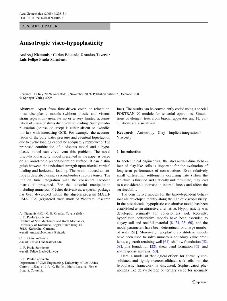
mentioned coefficients k and j. The reference values are
the creep rate (fluidity parameter) Dr = 1%/h, and the
reference states TB0 and eB0 on the primary compression
line (or reference isotach [59]) corresponding to the creep
rate Dr (see Fig. 1) or to the CRSN compression with
D ¼ kDr=ðk jÞ:The values e0 and T0 are needed only once to initialize
the incremental process. The parameters of the engineering
description can be shown [42] to be related to the
parameters
t0 ¼kIv
DrOCR1=Iv with OCR ¼ TB=T; ð5Þ
w ¼ kIv ð6Þ
of the 1-d model. These equations are obtained comparing
Eqs. 1–3 with Eq. 4 for the special cases.
4 Isotropic visco-hypoplasticity
The aforementioned 1-d model was generalized [42] using
hypoplasticity and OCR based on the isotropic preconsol-
idation surface of the modified Cam Clay Model (MCC).
The decomposition of the strain rate into elastic and vis-
cous portions D ¼ De þ Dvis was assumed. All irreversible
deformations were treated collectively as a time-dependent
variable Dvis: The viscous strain rate Dvis ¼ DvisðT; eÞ was
assumed to be a function of the Cauchy stress T and the
void ratio e. The Norton’s power rule [46] for the intensity
of viscous flow and the hypoplastic flow rule for its
λ1
(TB0,eB0)
(TB,e)
Dr
ln(TB)
ln(1+e)
ref. isotach
λ1
ln(T )
ln(1+e)
κ1
Fig. 1 Reference values TB0, eB0 defined on the reference isotach
(corresponding to Dr) and coefficients k and j
Acta Geotechnica (2009) 4:293–314 295
123
direction were adopted. The hypoplastic flow rule
DvismðTÞ and the hypoelastic barotropic stiffness E
were used as follows
T ¼ E : D Dvis
with Dvis ¼ mDrOCR1=Iv : ð7Þ
A hyperelastic stiffness based upon complementary
energy potentials [23] and similar to the model proposed by
[43], is planned in a future version of this model as a
replacement for the current E:
The definition of OCR has been generalized for non-
isotropic stresses based on MCC preconsolidation surface.
An analogous generalization based on the anisotropic
preconsolidation surface will be presented in the next
section, Eq. 39. The expression OCR1=Iv ; used as the
function for intensity of the creep, can be shown to be
analogous to the one proposed by Adachi and Oka [1, 2,
47]. Readers familiar with the old hypoplastic notation [21,
65] based on two tensorial functions
L ¼ E ¼ a2 FM
a
2
Iþ TT
!
ð8Þ
N ¼ a2 FM
aTþ T
ð9Þ
may find the following interrelations helpful:
E ¼ trT
3jL and m ¼ L1 : N
!; ð10Þ
wherein j denotes the swelling coefficient [15] taken from
lnðpÞ lnð1þ eÞ diagram, Fig. 1. In the above expressions
for E, the coefficients a and FM are defined as
FM ¼
ffiffiffiffiffiffiffiffiffiffiffiffiffiffiffiffiffiffiffiffiffiffiffiffiffiffiffiffiffiffiffiffiffiffiffiffiffiffiffiffiffiffiffiffiffiffiffiffiffiffiffiffiffiffiffiffiffiffiffiffiffi
1
8tan2 Wþ 2 tan2 W
2þffiffiffi
2p
tan W cos 3h
s
1
2ffiffiffi
2p tan W
ð11Þ
with
a ¼ffiffiffi
3p
3 sin ucð Þ2ffiffiffi
2p
sin uc
; tan W ¼ffiffiffi
3pjjTjj; ð12Þ
and h is the Lode’s angle given in Eq. 43. Note that the
‘‘hypoelastic’’ stiffness depends on the critical friction
angle uc.
The small-strain constitutive behaviour described with
the so-called intergranular strain [44] is left out in the
current anisotropic version for brevity. A future version of
the model should consider the small strain stiffness effects
[9,14, 26, 33, 55, 56, 42, 44]. The isotropic visco-hypo-
plasticity is extensively discussed in [42], and it has been
used in numerous FE applications. Here, we concentrate on
the anisotropic preconsolidation surface and on the implicit
time integration strategy only.
5 Anisotropic model
From numerical tests [57], it can be concluded that the
isotropic model [42] requires an anisotropic extension,
especially for a better fit of the biaxial test results on K0
consolidated samples [63]. This can be achieved using
anisotropic functions for OCR and for the unit tensor m
defining the flow rule. A well-known anisotropic effect of
naturally consolidated soils manifests itself in the
undrained shear tests. The undrained shear strength cu turns
out to be significantly greater for triaxial compression than
for extension, and this effect cannot be explained by the
different inclinations of the critical state lines MC ¼ 6 sin uc
3sin uc
and ME ¼ 6 sin uc
3þsin uc; respectively.
The main constitutive equation of the new model takes
the form similar to Eq. 7
T ¼ E : D Dvis DHp
with ð13Þ
Dvis ¼ mDr OCR1=Iv and DHp ¼ C1mjjDjj ð14Þ
Apart from the anisotropic functions for OCR and for the
flow rule m, Eq. 13 introduces a small-term C1E : mjjDjjwith a material constant C1 & 0.1 or less. Upon 1-d strain
cycles (so called in-phase cycles), the hypoelastic2 linear
term E : D causes no accumulation of stress. The term
C1E : mjjDjj causes accumulation dependent on m and on
the length of the strain pathR
jjDjjdt: One may call it
pseudo-relaxation, but since
DHp ¼ C1mjjDjj ð15Þ
resembles the hypoplastic nonlinear term we prefer to call
DHp the hypoplastic strain and C1E : mjjDjj the hypo-
plastic relaxation. Note that the rates Dvis and DHp are
parallel, and both are functions of the current state
described by stress T and the equivalent stress TB (see the
next subsection). The essential difference between Dvis
and DHp is that the hypoplastic strain is driven by the
magnitude of the deformation, whereas the viscous strain
is driven by time t.
5.1 One-dimensional version of the novel model
The effect of the hypoplastic strain DHp can be examined in
one-dimensional case using DHp ¼ C1jDj: The aniso-
tropy of the yield surface and of the flow are not relevant,
of course.
2 The hyperelastic stiffness is conservative in the sense that anyclosed strain cycle causes a closed stress cycle and vice versa. For
hypoelastic formulations, this is true for in-phase cycles only, e.g.
ðtÞ ¼ sinðtÞampl: The out-of-phase strain cycles, e.g. with 11 ¼ampl
11 sinðtÞ and 22 ¼ ampl22 sinðt þ p=3Þ may lead to undesired accu-
mulation of stress. The direction of accumulation depends on the
sense of rotation ( or ).
296 Acta Geotechnica (2009) 4:293–314
123
From
_T ¼ Tj ðD Dvis DHpÞ
Dvis ¼ DrTTB
1=Iv
DHp ¼ C1jDjTB ¼ TB0
1þe1þeB0
1=kor _TB ¼ TBD
k
8
>
>
>
>
>
<
>
>
>
>
>
:
ð16Þ
one may obtain the following special cases:
• During pure creep _T 0 from the first equation of
Eq. 16 follows Dþ C1jDj ¼ Dvis and since C1 1
holds, we conclude that D and Dvis have the same
sign (both are negative = compressive) and therefore
|D| = -D. We obtain, therefore, a slightly larger value
of the creep rate
D ¼ 1
1 C1
Dvis ð17Þ
compared to D ¼ Dvis in the original model Eq. 4.
• The pure relaxation is obtained substituting D : 0 into
the first equation of Eq. 16. We obtain
_T ¼ T
jDvis [ 0 ð18Þ
which is identical to the relaxation rate from the ori-
ginal model Eq. 4.
• Let us assume a constant compressive creep rate Dvis ¼const\0: We examine the implications of _Dvis ¼ 0:
Judging by the second equation of Eq. 16 (for T = 0
and TB = 0, of course), the constant rate of creep
requires
T
TB
¼ 0 or _T=T ¼ _TB=TB ð19Þ
In the latter form, we may substitute _TB=TB ¼ D=k from
the last equation of Eq. 16 and j _T=T ¼ D Dvis þ C1jDjfrom the first equation of Eq. 16. This leads to
1
jD Dvis þ C1jDj
¼ D=k ð20Þ
Assumption D [ 0 would result in Dvis=D ¼ 1 j=kþC1 which cannot be satisfied for Dvis\0 because 1j=kþ C1 [ 0 holds. Therefore, D must be negative and
hence
D ¼ Dvis 1 j=k C1½ 1¼ const\0 ð21Þ
Equation (21) shows that our initial assumption about the
viscous strain Dvis ¼ const\0 implies a compression with
a constant strain rate deformation. The rate of
deformation is slightly different from D ¼ Dvisk=ðk jÞobtained analogously [42] from Eq. 4. The relation
between the stress rate and the strain rate for such case
is obtained by elimination of Dvis in the first equation of
Eq. 16 using Eq. 21.
_T ¼ T
jðDþ C1jDj DvisÞ with D\0 ð22Þ
_T ¼ T
jð1 C1 1 j=k C1½ ÞD ð23Þ
_T ¼ T
kD ð24Þ
After time integration, this relation can be represented by a
straight line parallel to the reference isotach in the com-
pression diagram in Fig. 1.
5.2 Anisotropic preconsolidation surface
and the flow rule
The anisotropy of visco-hypoplastic model follows from
the equation of the preconsolidation surface. In the new
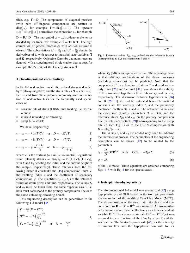
model, the preconsolidation surface has the form of an
inclined ellipse in the p-q space, Fig. 2 or an ellipsoid in
the principal stress space Fig. 4. The tensorial equation of
the preconsolidation surface has the form
FðT;X; pBÞ M2p2 3MpT : Xþ 3
2T : T
þM2ppB3
2X : X 1
¼ 0:ð25Þ
The equivalent pressure of the isotropic MCC model is
replaced by the preloading stress
TB ¼ pBð1þXMXÞ; ð26Þ
see Fig. 2.
Note that a simple rotation of the Cam clay preconsol-
idation ellipse would not satisfy the isochoric flow condi-
tion for critical state [27].
The size of the ellipse is described by the scalar state
variable pB, and the obliquity is described by the deviatoric
p=-(T1+2T3)
q=-(T1-T3)MC
1
ME
1
pB
TB
pB+
F=0 T 1ΩMΩ
Fig. 2 Anisotropic preconsolidation surface F = 0 and the definition
of pB? for the current stress T. The axisymmetric stress T and the
axisymmetric structure tensor X can be represented in the common
p-q diagram
Acta Geotechnica (2009) 4:293–314 297
123

structural tensor X; similar to the model introduced by
Dafalias [18]. Keeping X ¼ 0; we enforce isotropic pre-
consolidation because the main diameter of the ellipse
remains on the hydrostatic axis. The slope of the critical
surface in the p-q diagram is described by M = M(h)
which depends on the critical friction angle and is a
function of the Lode’s angle hðTÞ of stress discussed fur-
ther in this section (in the Drucker–Prager model M would
be a material constant). The condition q2 ¼ M2p2 of criti-
cal state can be expressed in general case as
FcritðTÞ 3
2T : T M2p2 ¼ 0 ð27Þ
For triaxial compression, M(h) reaches the maximum
MC ¼ 6 sin uc
3sin uc: For triaxial extension, M(h) reaches the
minimum ME ¼ 6 sin uc
3þsin uc: Additionally, we introduce MX
which denotes the critical slope for h dictated by the cur-
rent X: In general, M 6¼ MX: The critical state is assumed
to be isotropic, independent of stress T and of deformation
history X; contrarily to [39, 67].
Equation (25) of the preconsolidation surface has been
derived from the general equation of an ellipse
f ðp; qÞ p2 þ l1pqþ l2q2 þ l3pþ l4qþ l5 ¼ 0 ð28Þ
in the space of normalized Roscoe components p ¼ p=pB
and q ¼ q=ðMpBÞ: The following requirements have been
imposed:
f ð0; 0Þ ¼ 0 l5 ¼ 0 ð29Þf;qð0; 0Þ ¼ 0 l4 ¼ 0 ð30Þ
f ð1;xÞ ¼ 0 1þ l1xþ l2x2 þ l3 ¼ 0 ð31Þ
f;qð1;xÞ ¼ 0 l1 ¼ 2l2x ð32Þ
meaning that the ellipse should pass through the points
ðp; qÞ ¼ ð0; 0Þ and (1, x) having the outer normal parallel
to the p-axis there. Moreover, we require
f;qðp; pÞ ¼ 0 for f ðp; pÞ ¼ 0 l2 ¼ 1 ð33Þ
f;qðp;pÞ ¼ 0 for f ðp;pÞ ¼ 0 l2 ¼ 1 ð34Þ
meaning that on crossing with the critical state lines
p ¼ q the ellipse f ðp;pÞ ¼ 0 should have the outer
normal parallel to the q-axis: These features of the
preconsolidation surface are not always satisfied by
models in the literature, for instance [27, 32]. All these
conditions lead to the preconsolidation surface
f ðp; qÞ p2 2xpqþ q2 ð1 x2Þp ¼ 0 or ð35ÞFðp; q;x; pBÞ M2p2 2Mpxqþ q2
M2ppBð1 x2Þ ¼ 0;ð36Þ
wherein the second equation has been obtained using
the definitions of p and q and multiplying f with (pB M)2.
The tensorial form Eq. 25 results from the definition of the
Roscoe’s deviatoric invariant: q2 ¼ 32
T : T;x2 ¼ 32X : X
and qx ¼ 32
T : X.
Analogous conditions imposed onto the preconsolida-
tion surface FðT;X; pBÞ given in Eq. 25 and on its outer
normal
F0 ¼ 3T 3pMX 2M2p 3MX : T
þM2pB3
2X : X 1
1
31þ oF
oMM0
ð37Þ
are satisfied:
• Fð0;X; pBÞ ¼ 0
• F0ð0;X; pBÞ 1; note that oF=oM ¼ 0 in this case
• FðTB;X; pBÞ ¼ 0; note that M ¼ MX for T ¼ TB:
• F0ðTB;X; pBÞ 1; note that qF/qM = 0 in this case
• For intersection line of surfaces FcritðTÞ ¼ 0 and
FðT;X; pBÞ ¼ 0 given by Eqs. 25 and 27, respectively,
holds the isochoric flow rule
1 : F0ðTB;X; pBÞ ¼ 0 ð38Þ
One can easily show that the expression in square
brackets in Eq. 37 multiplied with p is . . .½ p ¼ F Fcrit; so
the volumetric portion of the outer normal F0 must indeed
vanish if F and Fcrit simultaneously do.
We intend to replace the hyperellipse Eq. 25 by the
alternative formulation Eq. 51 in future. This function not
only guarantees to satisfy the isochoric flow rule in the
critical state exactly but also keeps all principal stresses
negative.
Similar strain-induced anisotropic yield surfaces have
been used in numerous elasto-plastic soil models (e.g. [19,
30, 64]). Contrary to the elastoplastic yield surfaces,
however, the surface Eq. 25 can be surpassed by the stress
path.
The preconsolidation surface Eq. 25 can be shown to be
orthotropic with the orthotropy axis coinciding with the
principal directions of X: If required by experimental data,
the mathematical form of Eq. 25 can be extended in future
according to representation theorems. An example of such
systematic approach for transversally isotropic soils is
given in [11].
The overconsolidation ratio OCR describes the ‘‘dis-
tance’’ from the current stress T to the preconsolidation
surface. Stresses inside the preconsolidation surface corre-
spond to F \ 0 and OCR [ 1. Stresses outside correspond
to F [ 0 and OCR \ 1. In the case F = 0 or equivalently
OCR = 1, stresses lie on the preconsolidation surface, and
the intensity of creep jjDvisjj takes referential value
jjDvisjj ¼ Dr which is evident from Eq. 14 for OCR=1. The
corresponding creep rate is jjDjj ¼ Dr=ð1 C1Þ Dr:
The rate of the viscous strain rate Dvis depends strongly
on the distance between the current stress and the pre-
consolidation surface. The intensity of the viscous strain
298 Acta Geotechnica (2009) 4:293–314
123
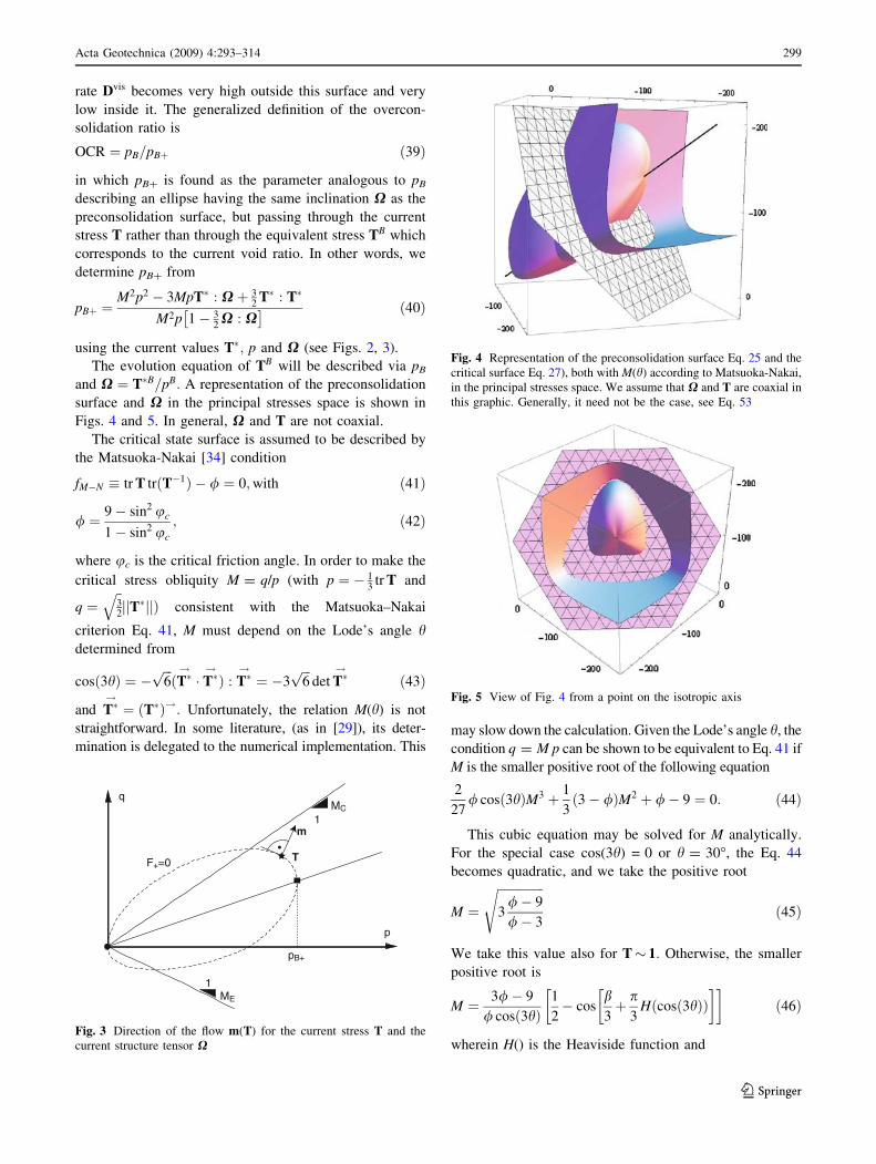
rate Dvis becomes very high outside this surface and very
low inside it. The generalized definition of the overcon-
solidation ratio is
OCR ¼ pB=pBþ ð39Þ
in which pB? is found as the parameter analogous to pB
describing an ellipse having the same inclination X as the
preconsolidation surface, but passing through the current
stress T rather than through the equivalent stress TB which
corresponds to the current void ratio. In other words, we
determine pB? from
pBþ ¼M2p2 3MpT : Xþ 3
2T : T
M2p 1 32X : X
ð40Þ
using the current values T; p and X (see Figs. 2, 3).
The evolution equation of TB will be described via pB
and X ¼ TB=pB: A representation of the preconsolidation
surface and X in the principal stresses space is shown in
Figs. 4 and 5. In general, X and T are not coaxial.
The critical state surface is assumed to be described by
the Matsuoka-Nakai [34] condition
fMN tr T trðT1Þ / ¼ 0;with ð41Þ
/ ¼ 9 sin2 uc
1 sin2 uc
; ð42Þ
where uc is the critical friction angle. In order to make the
critical stress obliquity M = q/p (with p ¼ 13
tr T and
q ¼ffiffi
32
q
jjTjjÞ consistent with the Matsuoka–Nakai
criterion Eq. 41, M must depend on the Lode’s angle hdetermined from
cos 3hð Þ ¼ ffiffiffi
6pðT! T!Þ : T!¼ 3
ffiffiffi
6p
det T!
ð43Þ
and T!¼ ðTÞ!: Unfortunately, the relation M(h) is not
straightforward. In some literature, (as in [29]), its deter-
mination is delegated to the numerical implementation. Thismay slow down the calculation. Given the Lode’s angle h, the
condition q = M p can be shown to be equivalent to Eq. 41 if
M is the smaller positive root of the following equation
2
27/ cos 3hð ÞM3 þ 1
33 /ð ÞM2 þ / 9 ¼ 0: ð44Þ
This cubic equation may be solved for M analytically.
For the special case cos(3h) = 0 or h = 30, the Eq. 44
becomes quadratic, and we take the positive root
M ¼
ffiffiffiffiffiffiffiffiffiffiffiffiffiffiffi
3/ 9
/ 3
s
ð45Þ
We take this value also for T 1: Otherwise, the smaller
positive root is
M ¼ 3/ 9
/ cosð3hÞ1
2 cos
b3þ p
3Hðcosð3hÞÞ
ð46Þ
wherein H() is the Heaviside function and
MC
1
ME
1
pB+
F+=0 T
m
p
q
Fig. 3 Direction of the flow m(T) for the current stress T and the
current structure tensor X
Fig. 4 Representation of the preconsolidation surface Eq. 25 and the
critical surface Eq. 27), both with M(h) according to Matsuoka-Nakai,
in the principal stresses space. We assume that X and T are coaxial in
this graphic. Generally, it need not be the case, see Eq. 53
Fig. 5 View of Fig. 4 from a point on the isotropic axis
Acta Geotechnica (2009) 4:293–314 299
123

b ¼ arccos sign cosð3hÞ½ b
ð3þ /Þ3
( )
with ð47Þ
b ¼ 27þ 27/ 9/2 þ 18 cos2ð3hÞ/2 þ /3
2 cos2ð3hÞ/3 ð48Þ
The analytical expression Eq. 47 is relatively
complicated, and M changes slowly with T. Therefore, in
the Newton iteration procedures that follow, we will assume
M0 0 ð49Þ
The cost of computation of M0 is expected to be high
compared to some marginal increase in the convergence
rates.
The flow rule m needs to be defined for an arbitrary
stress T and not just for stresses on the yield surface as it is
the case in elastoplasticity. For this purpose, we propose
the following procedure. First, the preconsolidation pres-
sure pB? is found from FðT;X; pBþÞ ¼ 0 for the current T
and X: Next, an auxiliary surface (dashed ellipse in Fig. 2)
FþðTÞ ¼ FðT;X; pBþÞ ¼ 0 is constructed. Finally, the
direction of flow follows from
m ¼ F0þ
!¼ oFþ
oT
!
pBþ
ð50Þ
wherein pB? and X are constant, and the analytical
expression for the Frechet derivative F0þ!
is given in Eq. 72
in Sect. 6.2. In other words, we construct a hypothetical
preconsolidation surface (dashed ellipse in Fig. 2) passing
through the current stress T and affine to the current pre-
consolidation surface (solid-line ellipse in Fig. 2). Then,
we calculate m as a unit outer normal to this surface (the
associated flow rule with respect to FþðTÞ ¼ 0Þ:Small deviations from AFR are allowed for [40], and
such a non-associated flow rule (NAFR) may be necessary
in a future version of the model in order to satisfy the
condition of isochoric flow direction in the critical state.
As an unpleasant consequence of the consistency of the
critical stress ratio M(h) with the Matsuoka–Nakai crite-
rion, the preconsolidation surface becomes slightly con-
cave near the isotropic axis, see Fig. 4 and tensile stresses
(tr T\0 but one of the principal stresses may become
positive) can be reached at very low pressures.
In order to remove these shortcomings, an alternative
preconsolidation surface
GðT;X; pBÞ tr TXð Þtr TX½ 1
/ ¼ 0ð51Þ
with
/ ¼ /max 1 p
pB
þ 9p
pBð52Þ
and /max [ 9 is currently being studied (e.g. see Fig. 6).
Such surfaces are smooth, have no concavity and are
bounded to the compressive stresses.
5.3 Evolution of state variables X and pB
The evolution equations of the preconsolidation stress TB
are provided separately for pB and for X: The evolution of
the structural deviatoric tensor X
is proposed to be
X ¼ C2 C3ðTÞ 1
3M X
OCR1=Iv
htr Dihtr mið53Þ
We do not follow the idea [20, 41] that relates the evolution
of the anisotropy tensor X to the plastic strain deformation
alone, because it implies evolution of X for critical state
flow. The length of such process cannot influence the
structure. In our opinion, the evolution of X is possible
upon contractant strain paths only, i.e. only for tr D\0; and
for subcritical stress states (tr m\0Þ: The rate of this
evolution increases rapidly with decreasing OCR. Since
Fig. 6 Preconsolidation surface Eq. 52 based on the Matsuoka-Nakai function with /(p)
300 Acta Geotechnica (2009) 4:293–314
123
Iv & 0.05, the evolution of X is practically absent at
OCR [ 1.5. In this case, the multiplier OCR1=Iv 3104
makes X almost negligible. The direction of X is dictated
by the difference between the current stress deviator T and
X (both appropriately scaled). The scalar multipliers at X
and T are chosen to reproduce the asymptotic behaviour
upon radial compression tests, i.e. those with tr D\0 and
T ¼ const: The asymptotic value of the structural tensor
is in such case X ¼ ð3C3
M TÞ: The material parameter
C3 can be easily found making the direction of flow m
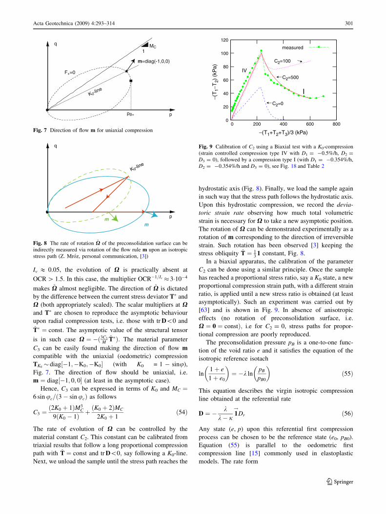
compatible with the uniaxial (oedometric) compression
TK0 diag½1;K0;K0 (with K0 = 1 - sinu),
Fig. 7. The direction of flow should be uniaxial, i.e.
m ¼ diag½1; 0; 0 (at least in the asymptotic case).
Hence, C3 can be expressed in terms of K0 and MC ¼6 sin uc=ð3 sin ucÞ as follows
C3 ¼ð2K0 þ 1ÞM3
C
9ðK0 1Þ þðK0 þ 2ÞMC
2K0 þ 1ð54Þ
The rate of evolution of X can be controlled by the
material constant C2. This constant can be calibrated from
triaxial results that follow a long proportional compression
path with T ¼ const and tr D\0; say following a K0-line.
Next, we unload the sample until the stress path reaches the
hydrostatic axis (Fig. 8). Finally, we load the sample again
in such way that the stress path follows the hydrostatic axis.
Upon this hydrostatic compression, we record the devia-
toric strain rate observing how much total volumetric
strain is necessary for X to take a new asymptotic position.
The rotation of X can be demonstrated experimentally as a
rotation of m corresponding to the direction of irreversible
strain. Such rotation has been observed [3] keeping the
stress obliquity T ¼ 13
1 constant, Fig. 8.
In a biaxial apparatus, the calibration of the parameter
C2 can be done using a similar principle. Once the sample
has reached a proportional stress ratio, say a K0 state, a new
proportional compression strain path, with a different strain
ratio, is applied until a new stress ratio is obtained (at least
asymptotically). Such an experiment was carried out by
[63] and is shown in Fig. 9. In absence of anisotropic
effects (no rotation of preconsolidation surface, i.e.
X ¼ 0 ¼ constÞ; i.e for C2 = 0, stress paths for propor-
tional compression are poorly reproduced.
The preconsolidation pressure pB is a one-to-one func-
tion of the void ratio e and it satisfies the equation of the
isotropic reference isotach
ln1þ e
1þ e0
¼ k lnpB
pB0
ð55Þ
This equation describes the virgin isotropic compression
line obtained at the referential rate
D ¼ kk j
1!
Dr ð56Þ
Any state (e, p) upon this referential first compression
process can be chosen to be the reference state (e0, pB0).
Equation (55) is parallel to the oedometric first
compression line [15] commonly used in elastoplastic
models. The rate form
MC1
pB+
F+=0
m=diag(-1,0,0)
p
q
K0-line
Fig. 7 Direction of flow m for uniaxial compression
p
q
K0-line
mm
Fig. 8 The rate of rotation X of the preconsolidation surface can be
indirectly measured via rotation of the flow rule m upon an isotropic
stress path (Z. Mroz, personal communication, [3])
0
20
40
60
80
100
120
0 200 400 600 800
−(T
1−T
2) (
kPa)
−(T1+T2+T3)/3 (kPa)
measured
C2=500
C2=100
C2=0
IV
I
Fig. 9 Calibration of C2 using a Biaxial test with a K0-compression
(strain controlled compression type IV with D1 = -0.5%/h, D2 =
D3 = 0), followed by a compression type I (with D1 = -0.354%/h,
D2 = -0.354%/h and D3 = 0), see Fig. 18 and Table 2
Acta Geotechnica (2009) 4:293–314 301
123
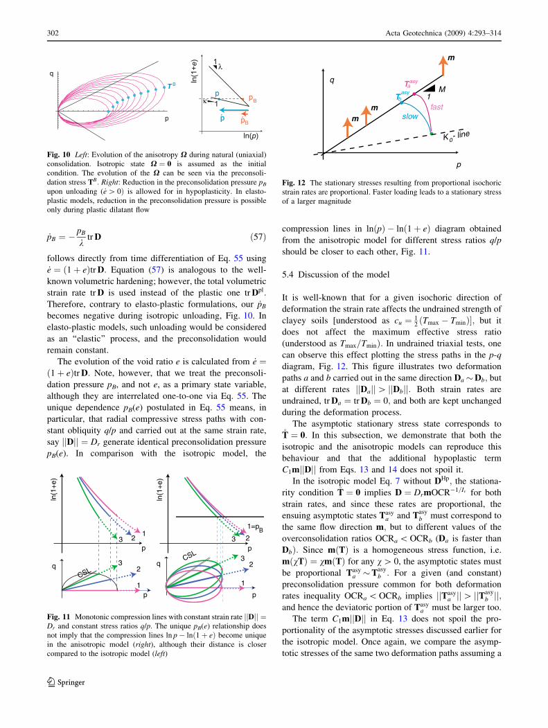
_pB ¼ pB
ktr D ð57Þ
follows directly from time differentiation of Eq. 55 using
_e ¼ ð1þ eÞtr D: Equation (57) is analogous to the well-
known volumetric hardening; however, the total volumetric
strain rate tr D is used instead of the plastic one tr Dpl:
Therefore, contrary to elasto-plastic formulations, our _pB
becomes negative during isotropic unloading, Fig. 10. In
elasto-plastic models, such unloading would be considered
as an ‘‘elastic’’ process, and the preconsolidation would
remain constant.
The evolution of the void ratio e is calculated from _e ¼ð1þ eÞtr D: Note, however, that we treat the preconsoli-
dation pressure pB, and not e, as a primary state variable,
although they are interrelated one-to-one via Eq. 55. The
unique dependence pB(e) postulated in Eq. 55 means, in
particular, that radial compressive stress paths with con-
stant obliquity q/p and carried out at the same strain rate,
say jjDjj ¼ Dr generate identical preconsolidation pressure
pB(e). In comparison with the isotropic model, the
compression lines in lnðpÞ lnð1þ eÞ diagram obtained
from the anisotropic model for different stress ratios q/p
should be closer to each other, Fig. 11.
5.4 Discussion of the model
It is well-known that for a given isochoric direction of
deformation the strain rate affects the undrained strength of
clayey soils [understood as cu ¼ 12ðTmax TminÞ; but it
does not affect the maximum effective stress ratio
(understood as Tmax=TminÞ: In undrained triaxial tests, one
can observe this effect plotting the stress paths in the p-q
diagram, Fig. 12. This figure illustrates two deformation
paths a and b carried out in the same direction DaDb; but
at different rates jjDajj[ jjDbjj: Both strain rates are
undrained, tr Da ¼ tr Db ¼ 0; and both are kept unchanged
during the deformation process.
The asymptotic stationary stress state corresponds toT ¼ 0: In this subsection, we demonstrate that both the
isotropic and the anisotropic models can reproduce this
behaviour and that the additional hypoplastic term
C1mjjDjj from Eqs. 13 and 14 does not spoil it.
In the isotropic model Eq. 7 without DHp; the stationa-
rity condition T ¼ 0 implies D ¼ DrmOCR1=Iv for both
strain rates, and since these rates are proportional, the
ensuing asymptotic states Tasya and Tasy
b must correspond to
the same flow direction m; but to different values of the
overconsolidation ratios OCRa \ OCRb (Da is faster than
DbÞ: Since mðTÞ is a homogeneous stress function, i.e.
mðvTÞ ¼ vmðTÞ for any v[ 0, the asymptotic states must
be proportional Tasya Tasy
b : For a given (and constant)
preconsolidation pressure common for both deformation
rates inequality OCRa \ OCRb implies jjTasya jj[ jjT
asyb jj;
and hence the deviatoric portion of Tasya must be larger too.
The term C1mjjDjj in Eq. 13 does not spoil the pro-
portionality of the asymptotic stresses discussed earlier for
the isotropic model. Once again, we compare the asymp-
totic stresses of the same two deformation paths assuming a
p
q
T B
λ1
ln(p)
ln(1+e
)
κ 1p
B
pB
pp
pp
Fig. 10 Left: Evolution of the anisotropy X during natural (uniaxial)
consolidation. Isotropic state X ¼ 0 is assumed as the initial
condition. The evolution of the X can be seen via the preconsoli-
dation stress TB: Right: Reduction in the preconsolidation pressure pB
upon unloading ( _e [ 0Þ is allowed for in hypoplasticity. In elasto-
plastic models, reduction in the preconsolidation pressure is possible
only during plastic dilatant flow
ln(1
+e)
q
p
p
CSL
1
1
2
2
3
3
ln(1
+e)
q
p
pCSL
1
1=p
2
2
3
3B
Fig. 11 Monotonic compression lines with constant strain rate jjDjj ¼Dr and constant stress ratios q/p. The unique pB(e) relationship does
not imply that the compression lines ln p lnð1þ eÞ become unique
in the anisotropic model (right), although their distance is closer
compared to the isotropic model (left)
p
q
1M
K - line0
slowfast
T
Tasy
asya
b
mm
m
Fig. 12 The stationary stresses resulting from proportional isochoric
strain rates are proportional. Faster loading leads to a stationary stress
of a larger magnitude
302 Acta Geotechnica (2009) 4:293–314
123
common initial stress and a common preconsolidation TB:
Note that TB remains constant during any isochoric
deformation. Indeed, according to Eqs. 53 and 57, neither
X nor pB may change while tr D ¼ 0:
In the anisotropic model Eq. 13 with DHp 6¼ 0; the sta-
tionarity condition T ¼ 0 leads to
DmDrOCR1=Iv mC1jjDjj ¼ 0 ð58Þ
from which we may conclude that the required common
flow rule is m ¼ D!
a ¼ D!
b: Recall that Da and Db are pro-
portional. Hence, using the homogeneity of the flow rule
(for a given and constant TBÞ with respect to stress, we infer
that the asymptotic stresses are proportional Tasya Tasy
b :
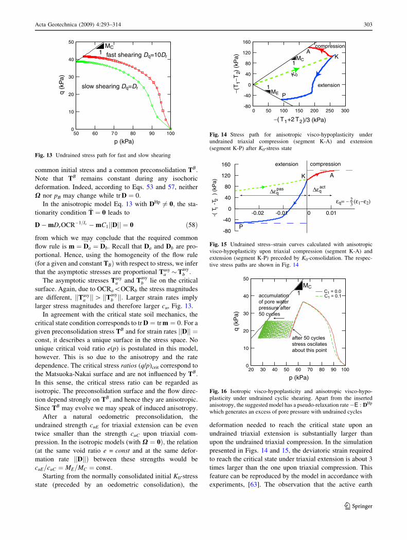
The asymptotic stresses Tasya and Tasy
b lie on the critical
surface. Again, due to OCRa\OCRb the stress magnitudes
are different, jjTasya jj[ jjT
asyb jj: Larger strain rates imply
larger stress magnitudes and therefore larger cu, Fig. 13.
In agreement with the critical state soil mechanics, the
critical state condition corresponds to tr D ¼ tr m ¼ 0: For a
given preconsolidation stress TB and for strain rates jjDjj ¼const; it describes a unique surface in the stress space. No
unique critical void ratio e(p) is postulated in this model,
however. This is so due to the anisotropy and the rate
dependence. The critical stress ratios (q/p)crit correspond to
the Matsuoka-Nakai surface and are not influenced by TB:
In this sense, the critical stress ratio can be regarded as
isotropic. The preconsolidation surface and the flow direc-
tion depend strongly on TB; and hence they are anisotropic.
Since TB may evolve we may speak of induced anisotropy.
After a natural oedometric preconsolidation, the
undrained strength cuE for triaxial extension can be even
twice smaller than the strength cuC upon triaxial com-
pression. In the isotropic models (with X ¼ 0Þ; the relation
(at the same void ratio e = const and at the same defor-
mation rate jjDjjÞ between these strengths would be
cuE=cuC ¼ ME=MC ¼ const:
Starting from the normally consolidated initial K0-stress
state (preceded by an oedometric consolidation), the
deformation needed to reach the critical state upon an
undrained triaxial extension is substantially larger than
upon the undrained triaxial compression. In the simulation
presented in Figs. 14 and 15, the deviatoric strain required
to reach the critical state under triaxial extension is about 3
times larger than the one upon triaxial compression. This
feature can be reproduced by the model in accordance with
experiments, [63]. The observation that the active earth
0
10
20
30
40
50
50 60 7 0 80 90 100
q (k
Pa)
p (kPa)
MC1 fast shearing Dq=10Dr
slow shearing Dq=Dr
Fig. 13 Undrained stress path for fast and slow shearing
compression
-80
-40
0
40
80
120
160
0 50 100 150 200 250 300
−(T
1−T
2) (
kPa)
−( T1+2 T2)/3 (kPa)
KA
P
extension
K0
MC1
ME1
Fig. 14 Stress path for anisotropic visco-hypoplasticity under
undrained triaxial compression (segment K-A) and extension
(segment K-P) after K0-stress state
extension compression
-80
-40
0
40
80
120
160
-0.02 -0.01 0 0.01-(T 1
-T2
) (k
Pa)
K A
P
3 (ε1−ε2)−2−εq=
∆εqact
∆εqpas
Fig. 15 Undrained stress–strain curves calculated with anisotropic
visco-hypoplasticity upon triaxial compression (segment K-A) and
extension (segment K-P) preceded by K0-consolidation. The respec-
tive stress paths are shown in Fig. 14
0
10
20
30
40
50
20 30 40 50 60 70 80 90 100
q (k
Pa)
p (kPa)
1MC
C1 = 0.1
after 50 cycles stress oscilates about this point
accumulation of pore waterpressure after 50 cycles
C1 = 0.0
Fig. 16 Isotropic visco-hypoplasticity and anisotropic visco-hypo-
plasticity under undrained cyclic shearing. Apart from the inserted
anisotropy, the suggested model has a pseudo-relaxation rateE : DHp
which generates an excess of pore pressure with undrained cycles
Acta Geotechnica (2009) 4:293–314 303
123
pressure is mobilized much faster than the passive one may
be expected to be correctly reproduced in FE simulations.
Small closed stress cycles generate an additional accu-
mulation of the deformation independently of creep. This
effect is considered using C1 [ 0 and was absent in the
previous model as demonstrated in Fig. 16.
6 Implicit integration of finite increments
The constitutive models supposed to be used in FE pro-
grams deal with finite increments of stress and strain rather
than their rates. Implicit integration (Euler backward) of
anisotropic soil models has also been recommended for
elastoplasticity [4], using the close-projection method. Let
us consider a time increment from tn to tn?1. Given the
state fTn;Xn; pBng at the beginning of the increment, the
strain increment D and the time increment Dt ¼ tnþ1 tn;
we must determine the values Tnþ1; Xnþ1 and pBn?1 at the
end of the increment (including the nonlinearities within
this single increment).
The main difficulty in the incremental formulation of the
constitutive model compared to the rate form Eqs. 7, 53
and 57 follows from the fact that the stiffness E; the pre-
consolidation pressure pB, the anisotropic tensor X and the
viscous strain rate Dvis used in Eqs. 7, 53 and 57 as ‘‘given’’
do not remain constant upon the increment. According to
the definitions Eqs. 39, 50 and 10, they change with stress,
and this change of stress is unknown itself. For reasons of
numerical stability of the time integration, the changes in
the state variables upon the increment should be taken into
account. From this point of view, it is safe to take the final
values of state variables, i.e. the ones at the end of incre-
ment (further denoted with the index tnþ1Þ rather than the
known ones tn from the beginning of the increment. The
advantage of such implicit (Euler backward) time inte-
gration over the explicit (Euler forward) integration was
already pointed out by Zienkiewicz [68] and Cormeau [17],
and can be here demonstrated comparing two implemen-
tations of the 1-d viscoplastic model. We combine Eq. 4
into a single expression for stress increment.
Tnþ1 Tn ¼Tn
jDe
1þ en DrDt
Tn
TB0
1Iv 1þ en
1þ eB0
1Ivk
" #
ð59Þ
The strain rate D is given as _e=ð1þ eÞ: All rates are written
as increments. In the explicit time integration, one uses the
stiffness and the viscous rate at the beginning of the
increment. Therefore, all quantities appearing on the right-
hand side are known (they pertain to time t), and the
calculation of Tn?1 can be performed directly. In the
analogous equation with implicit integration
Tnþ1 Tn ¼Tnþ1
j
De
1þ enþ1
DrDtTnþ1
TB0
1Iv
1þ enþ1
1þ eB0
1Ivk
" #
ð60Þ
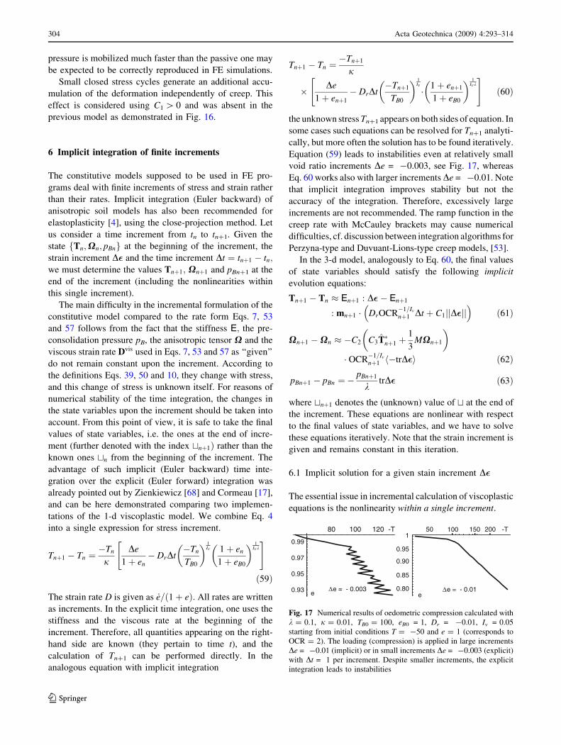
the unknown stress Tn?1 appears on both sides of equation. In
some cases such equations can be resolved for Tn?1 analyti-
cally, but more often the solution has to be found iteratively.
Equation (59) leads to instabilities even at relatively small
void ratio increments De = -0.003, see Fig. 17, whereas
Eq. 60 works also with larger increments De = -0.01. Note
that implicit integration improves stability but not the
accuracy of the integration. Therefore, excessively large
increments are not recommended. The ramp function in the
creep rate with McCauley brackets may cause numerical
difficulties, cf. discussion between integration algorithms for
Perzyna-type and Duvuant-Lions-type creep models, [53].
In the 3-d model, analogously to Eq. 60, the final values
of state variables should satisfy the following implicit
evolution equations:
Tnþ1 Tn Enþ1 : D Enþ1
: mnþ1 DrOCR1=Iv
nþ1 Dt þ C1jjDjj
ð61Þ
Xnþ1 Xn C2 C3Tnþ1 þ1
3MXnþ1
OCR1=Iv
nþ1 htrDi ð62Þ
pBnþ1 pBn ¼pBnþ1
ktrD ð63Þ
where tnþ1 denotes the (unknown) value of t at the end of
the increment. These equations are nonlinear with respect
to the final values of state variables, and we have to solve
these equations iteratively. Note that the strain increment is
given and remains constant in this iteration.
6.1 Implicit solution for a given stain increment D
The essential issue in incremental calculation of viscoplastic
equations is the nonlinearity within a single increment.
80 100 120
0.93
0.95
0.97
0.99
-T
∆e = - 0.003
1-T
ee ∆e = - 0.01
100 150 20050
0.95
0.90
0.85
0.80
Fig. 17 Numerical results of oedometric compression calculated with
k = 0.1, j = 0.01, TB0 = 100, eB0 = 1, Dr = -0.01, Iv = 0.05
starting from initial conditions T = -50 and e = 1 (corresponds to
OCR = 2). The loading (compression) is applied in large increments
De = -0.01 (implicit) or in small increments De = -0.003 (explicit)
with Dt = 1 per increment. Despite smaller increments, the explicit
integration leads to instabilities
304 Acta Geotechnica (2009) 4:293–314
123

The values of Tnþ1;Xnþ1 and pBn?1 appear on both
sides of Eqs. (61–63) being hidden in the expressions E; m
and OCR on the right-hand side. These equations will need
to be solved for the unknown tensors Tnþ1 and Xnþ1: The
third equation is also implicit, but it is sufficiently simple
(linear with respect to pBn?1) to be directly solved:
pBnþ1 ¼ 1þ 1
ktrD
1
pBn: ð64Þ
We start the process of iterative search for Tnþ1 and Xnþ1
by choosing the elastic predictor as an initial guess. In
other words, we choose Tnþ1 ¼ Tn þ DTel and Xnþ1 ¼ Xn
with DTel ¼ En : D: Next, this initial guess will be
improved adding corrections cT and cX to Tnþ1 and
Xnþ1; respectively. The corrections are obtained keeping
the strain increment D unchanged and minimizing the
errors rT ; rX resulting from usage of approximate values of
Tnþ1 and Xnþ1 in the evolution equations upon the
increment. From now on, we drop the n?1 index, so that
T and X denote the most recent approximations of Tnþ1
and Xnþ1: The following 12 independent components of
errors3 (due to symmetry Xij ¼ Xji and Tij ¼ TjiÞ may
appear:
rT ¼ T Tn E : D
þE : m DrOCR1=IvDt þ C1jjDjj
|fflfflfflfflfflfflfflfflfflfflfflfflfflfflfflfflfflfflfflfflfflfflfflfflzfflfflfflfflfflfflfflfflfflfflfflfflfflfflfflfflfflfflfflfflfflfflfflffl
A
rX ¼ XXn þ C2 C3T þ 13
MX
OCR1=Iv trDh i:
8
>
>
>
>
>
<
>
>
>
>
>
:
ð65Þ
Formally, we may see these errors as functions of T and X
and our intention is that these errors vanish after
corrections, i.e.
rTðTþ cT ;Xþ cXÞ ¼ 0rXðTþ cT ;Xþ cXÞ ¼ 0
ð66Þ
In the Newtonian iterative solution, one approximates the
above equations using the first terms of Taylor expansion
rTðTþ cT ;Xþ cXÞ rTðT;XÞ þ r0T : cT
þrT : cX 0rXðTþ cT ;Xþ cXÞ rXðT;XÞ þ r0X : cT
þrX : cX 0
8
>
>
<
>
>
:
ð67Þ
wherein dash and circle denote the Frechet derivatives with
respect to T and X; see the next subsection. All derivatives
are calculated using the most recent updated variables T;X
and with the final value of pB. For the Newton iteration
process we may construct the system of equations
rT ¼ r0T : cT þ rT : cX
rX ¼ r0X : cT þ rX : cX:
ð68Þ
Having solved this system numerically for cT and cX; we
add these corrections to the respective total values T, X:
The procedure requires the inversion of an unsymmetric
12 9 12 matrix containing the derivatives of the discrep-
ancies. This iteration process continues until the norms of
rT and rX are lower than some tolerance values.
An analogous iteration at constant D is known as the
Return Mapping Iteration (RMI) in elasto-plastic models. It
should not be mixed up with the equilibrium iteration (EI)
in which the strain increment is varied until the equilibrium
of stresses with external loads is reached.
6.2 Frechet derivatives
The calculation of derivatives that appear in Eq. 68 can be
tedious, and therefore we found them using an algebra pro-
gram MATHEMATICA [66] with the package nova.m devel-
oped by the first author4. In the RMI process, we need various
tensorial derivatives and the chain rules thereof. Starting with
the stiffness tensor E, we calculate its stress derivative as
E0 ¼ 1
3jE 1þtr T
3jE0 ð69Þ
with
E0ijklmn ¼ a2 TrrIijmnTkl þ TrrTijIklmn
ðTrrÞ3
2TijTkldmn
ðTrrÞ3þ 2
FM
aIijklF
0M mn
!
:
ð70Þ
We assume F0M 0 for simplicity. The stiffness E is
independent of X and hence E ¼ 0 holds. The flow rule m
is obtained for the updated stress T from FþðT; pBþ;XÞ ¼0 keeping the updated X constant, i.e.
mðT;XÞ ¼ F0þ
!ð71Þ
with
F0þ ¼ 3T 3pM X
þ 1
3M2pBþ
1
2M2pBþ X : X 2
3M2pþM X : T
1
ð72Þ
3 exactly 11 because Xii = 0.
4 nova.m can be downloaded from http://www.rz.uni-karlsruhe.
de/*gn99/. The expressionoTij
oTklð¼ IijklÞ can be calculated with
In 1½ :¼Needs 00Tensor‘nova‘00½ ;In 2½ :¼fD T i;j½ ;T k;l½ ½ Out 2½ :¼ðn Delta½ i;l½ n Delta½ j;k½ þn Delta½ i;k½ n Delta½ j;l½ Þ=2
The MATHEMATICA expressions enter directly in the code using a FOR-
TRAN-90 tensorial module. For example, the derivative of stress dis-
crepancy with respect to stress rT Eq. 86 can be coded in a single line
drTdO ¼ ðE:xx:ððm:out:dAdOÞ þ dmdO AÞÞ !rT ¼ E : ðmA þmAÞwhere the double contraction and the dyadic product are directly
evaluated using the operators.xx. and.out., respectively.
Acta Geotechnica (2009) 4:293–314 305
123
The total change in m with stress should take into account
the variability of pB? with stress which can be calculated
from
pBþ ¼ M2p3
2X : X 1
1
M2p2 3MpX : Tþ 3
2T : T
ð73Þ
as
p0Bþ ¼2M2 3
p2 T : T 9h i
1þ 18MX 18p T
3M2ð3X : X 2Þ ð74Þ
The correct stress derivative of m written as a function
mðT;X; pBþÞ is therefore found from the chain rule
m0 ¼ om
oTþ om
opBþp0Bþ
¼ 1
jjF0þjjJ F0þ
!F0þ
!
: F00þ þoF0þopBþ
p0Bþ
ð75Þ
wherein
oF0þopBþ
¼ 1
3M2 1
2M2X : X
1 ð76Þ
For the calculation of m0, we also need
F00þ ¼2
9M2 1
11þ 3IþMX1þM1X ð77Þ
Analogously, the partial derivative of the flow direction m
written as a function mðT;X; pBþÞ with respect to X
should take into account the variation of pB? with respect
to X; i.e.
m ¼ om
oXþ om
opBþpBþ
¼ 1
jjF0þjjJ F0þ
!F0þ
!
: F0þ þoF0þopBþ
pBþ
ð78Þ
wherein
F0þ ¼ M2pBþ1XþM1T 3MpI ð79Þ
and
pBþ ¼h1 h2Tþ h3Xð Þ with
h1 ¼ M2ð2 3X : XÞ2h i1
h2 ¼18MX : X 12M
h3 ¼ 36MX : T 54pþ 12M2pþ 18
pT : T
ð80Þ
The derivatives of the overconsolidation ratio OCR ¼pB=pBþ with respect to T and X are
OCR0 ¼ pB
ðpBþÞ2p0Bþ and OCR ¼ pB
ðpBþÞ2pBþ ð81Þ
It is convenient to define the scalar A that describes the
intensity of hypoplastic and the viscous strain rate:
A ¼ DrOCR1=IvDt þ C1jjDjj ð82Þ
Its derivatives, with respect to T and X are
A0 ¼ Dr
IvOCR 1=Ivþ1ð ÞDt OCR0 ð83Þ
A ¼ Dr
IvOCR 1=Ivþ1ð ÞDt OCR ð84Þ
Using the above partial derivatives the error in the stress
equation can be expressed as
rT ¼ T Tn E : Dþ E
: m DrOCR1=IvDt þ C1jjDjj
|fflfflfflfflfflfflfflfflfflfflfflfflfflfflfflfflfflfflfflfflfflfflfflfflzfflfflfflfflfflfflfflfflfflfflfflfflfflfflfflfflfflfflfflfflfflfflfflffl
A
ð85Þ
and its derivatives with respect to T and X are
r0T ¼ I E0:Dþ E0:mAþ E : mA0 þm0Að Þ ð86Þ
rT ¼ E : mA þmAð Þ ð87Þ
The error in the evolution equation of X is
rX¼XXnþC2 C3Tþ1
3MX
OCR1=Iv trDh i ð88Þ
and its derivatives with respect to T;X and pB are
r0X ¼ C2OCR1=Iv trDh ih i
C3
I T1
tr T 1
IvOCRC3T þ 1
3MX
OCR0
!
ð89Þ
rX ¼ Iþ C2OCR1=Iv trDh ih i
1
3MI 1
IvOCRC3T þ 1
3MX
OCR
ð90Þ
The errors rT ; rX from Eqs. 85 and 88 as well as their
derivatives r0T ; rT ; r0X; r
X from Eqs. 86, 87, 89 and Eq. 90
enter Eq. 68. This system can be converted to the matrix
form
r0T rTr0X rX
cT
cX
¼ rT
rX
ð91Þ
from which the corrections cT and cX can be calculated.
Derivatives r0T ; rT ; r0X; r
X appearing in Eq. 91 have been
converted analogously in the way a 3 9 3 9 3 9 3 stiff-
ness tensor would be converted to a 6 9 6 stiffness matrix.
The errors rT ; rX are both converted to ‘‘vectors’’ with six
components analogously in the way a 3 9 3 stress tensor
would be converted to a stress ‘‘vector’’. The six-compo-
nent correction ‘‘vectors’’ resulting from Eq. 91 must be
converted back to 3 9 3 tensors cT ; cX: However, doing
306 Acta Geotechnica (2009) 4:293–314
123
this back conversion, we must treat the corrections like
strains, i.e. their mixed components must be halved! A
conversion of second-order tensors to 9-component ‘‘vec-
tors’’ and fourth order tensors to 9 9 9 matrices is not a
good idea, because the resulting 18 9 18 matrix in Eq. 91
would be not only larger but also singular. Note that the
rows corresponding to mixed components, e.g. t12 and
t21; would be in this case identical.
6.3 The Jacobian dDT=dD
The Jacobian H ¼ dDT=dD is required for the efficient
equilibrium iteration on the FE-level, in particular when
the full Newton iteration strategy is used (as in ABAQUS/
Standard). In the implicit integration scheme, the tensor H,
should be calculated using the state variables T;X and pB
at the end of the increment and at the end of the RMI. In
order to find H we write out the equation for stress incre-
ment in the form
DT ¼ E : Dzfflfflffl|fflfflffl
A
E : mOCR1=Iv
zfflfflfflfflfflfflfflfflfflfflffl|fflfflfflfflfflfflfflfflfflfflffl
B
DrDt E : mjjDjjzfflfflfflfflfflfflffl|fflfflfflfflfflfflffl
C
C1
ð92Þ
It is convenient to distinguish the following subexpressions:
AðT;DÞ; BðT;X; pB; e;DÞ and CðT;X; pB; e;DÞ so that
the Jacobian can be written as
H ¼ dA
dD DrDt
dB
dD C1
dC
dDð93Þ
The derivatives of A, B and C with respect to D can be
computed via the derivatives with respect to T and X: For
simplicity, however, we disregard the derivative
dX=dD 0 while calculating H. Since the stress T is
one of the arguments of the functions A, B, C, it is
convenient to use the unknown as yet Jacobian H itself in
the chain-rule calculations via T, namely dt=dD ¼ t0 :
Hþ . . . : With these simplifications, we obtain
dA
dD¼ Eþ E0:D
: H ð94Þ
dB
dD¼ 1
IvOCR1=Iv1E : m
dOCR
dDþ OCR1=IvE :
dm
dD
þ OCR1=Iv E0:m
: H ð95Þ
dC
dD¼ E : mD
!þ jjDjjE :
dm
dDþ jjDjj E0:m
: H ð96Þ
Note that dDT=dD ¼ dT=dD because DT ¼ T Tn and
the initial stress Tn is constant. Moreover, for the sake of
simplicity, we assume oM=oT 0: Hence the following
approximations are obtained
dOCR
dD oOCR
opB
opB
oDþ oOCR
oT
oT
oD
¼ 1
kOCR1þ OCR0 : H ð97Þ
dm
dD om
oT
oT
oD¼ m0 : H ð98Þ
The substitution of Eqs. 97 and 98 into Eq. 95 results in
dB
dD¼ K : Hþ N ð99Þ
wherein
N ¼ 1
kIvOCR1=IvE : m 1 ð100Þ
OCR1=IvK ¼ 1
IvOCRE : mð ÞOCR0 þ E : m0 þ E0 : m
ð101Þ
Substituting Eq. 98 into Eq. 96 we obtain
oC
oD¼ R : Hþ S ð102Þ
wherein
R ¼ jjDjj E : m0 þ E0 : m
ð103Þ
S ¼ E : mD!
ð104Þ
The Eq. 93 can now be written as
I E0 : Dþ C1Rþ DrDtK
zfflfflfflfflfflfflfflfflfflfflfflfflfflfflfflfflfflfflfflfflfflfflfflfflffl|fflfflfflfflfflfflfflfflfflfflfflfflfflfflfflfflfflfflfflfflfflfflfflfflffl
W
: H ¼ E C1S DrDtNzfflfflfflfflfflfflfflfflfflfflfflfflfflffl|fflfflfflfflfflfflfflfflfflfflfflfflfflffl
Z
ð105Þ
and resolved for the Jacobian H
H ¼W1 : Z ð106Þ
Very few equilibrium iterations are necessary in the
numerical calculation with ABAQUS using this approxima-
tion of the Jacobian despite relatively large time steps.
7 Comparison with experimental results
The presented model has been implemented using the
constitutive FORTRAN 90 routine UMAT written in accor-
dance with the conventions of the FE Program ABAQUS
Standard. The same routine can be also linked with
INCREMENTALDRIVER5 to perform calculations of element
tests with stress or strain or mixed control of cartesian
components or combinations thereof.
5 INCREMENTALDRIVER is a program written by the first author to test
constitutive routines. Its open source code can be downloaded from
http://www.rz.uni-karlsruhe.de/*gn99/.
Acta Geotechnica (2009) 4:293–314 307
123
In order to verify the model, the results of biaxial tests
[63] on remoulded kaolin clay were simulated. The pre-
dictions were calculated with the set of material parameters
shown in Table 1. Other properties of the material are:
liquid limit wL = 48%, plastic limit wP = 18%, clay
fraction 59% and organic content 5.6%.
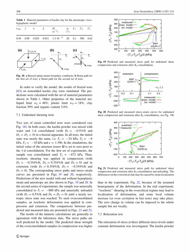
7.1 Undrained shearing tests
Two sets of strain controlled tests were considered (see
Fig. 18). In both cases, the kaolin powder was mixed with
water and 1-d consolidated (with D1 = -0.5%/h and
D2 = D3 = 0) in a biaxial apparatus. In all tests, the initial
state was nearly the same, i.e. T1 = -24 kPa, T2 = -8
kPa, T3 = -10 kPa and e = 1.396. In the simulations, the
initial value of the structure tensor X is set to zero prior to
the 1-d consolidation. For the first set of experiments, the
sample was consolidated until T1 = -672 kPa. Then,
isochoric shearing was applied in compression (with
D1 = -0.354%/h, D2 = 0.354%/h and D3 = 0) and in
extension (with D1 = 0.354%/h, D2 = -0.354%/h and
D3 = 0). The corresponding stress paths and stress–strain
curves are presented in Figs. 19 and 20, respectively.
Predictions of the new model with and without hypoplastic
strain and anisotropy are also shown in Figs. 19 and 20. In
the second series of experiments, the sample was uniaxially
consolidated to T1 = -800 kPa and uniaxially unloaded
(with D1 = 0.5%/h and D2 = D3 = 0) until a nearly iso-
tropic stress state was reached. To such overconsolidated
samples, an isochoric deformation was applied in com-
pression and extension. The comparisons between pre-
dicted and measured data are presented in Figs. 21 and 22.
The results of the numeric calculations are generally in
agreement with the laboratory data. The stress paths are
well predicted by the model. The predicted shear strength
of the overconsolidated samples in compression was higher
than in the experiment, Fig. 22, because of the assumed
homogeneity of the deformation. In the real experiment,
‘‘isochoric’’ shearing in the overcritical regime may lead to
localization of deformation, and some local volume
increase (or even cavitation in fast tests) may take place.
The zero change in volume can be imposed to the whole
sample but not locally.
7.2 Relaxation test
The relaxation of stress at three different stress levels under
constant deformation was investigated. The kaolin powder
Table 1 Material parameters of kaolin clay for the anisotropic visco-
hypoplastic model
e100 k j Iv Dr
(s-1)
uc
()
C1 C2 C3
0.94 0.09 0.025 0.031 1.310 -6 20 0.1 500 0.62
T1,D1
T2,D2
T3,D3=0
comp
ext
comp
extK0
K0
unload
(a) (b) (c)
Fig. 18 a Biaxial (plain strain) boundary conditions. b Strain path for
the first set of tests. c Strain path for the second set of tests
300
200
100
0
100
200
300
400
0 100 200 300 400 500 600
−(T
1−T
2) (
kPa)
−(T1+T2+T3)/3 (kPa)
measuredaniso. model
iso. model
Start(OCR=1)
Fig. 19 Predicted and measured stress path for undrained shear
compression and extension after K0 consolidation
-300
-200
-100
0
100
200
300
400
-0.2 -0.1 0.1 0.2
−(T 1
−T2)
(kPa
)
−ε1 (−)
aniso. modelmeasured
extension compression
start OCR=1
iso. model
Fig. 20 Predicted and measured stress-strain curves for undrained
shear compression and extension after K0 consolidation, see Fig. 18b
0
100
200
300
400
0 100 200 -200
-100
300 400 500 600 700
T1
2) (
kPa)
(T1+T2+T3)/3 (kPa)
predictedmeasured
Start(OCR=3)
Fig. 21 Predicted and measured stress path for undrained shear
compression and extension after K0 consolidation and unloading. The
differences on the overcritical side may be caused by strain localization
308 Acta Geotechnica (2009) 4:293–314
123

was mixed with water and 1-d consolidated in the biaxial
apparatus until a significant stress level was achieved. This
stress state (T1 = -22 kPa, T2 = T3 = -8 kPa) and void
ratio e = 1.4 are considered as the initial state. In the
simulation the tensor X is set to zero at the initial state. In a
first step, the sample was consolidated (with D1 = 0.5%/h
and D2 ¼ D3 ¼ 0) up to T1 = -108 kPa. In a second step,
the deformation was kept constant (D1 ¼ D2 ¼ D3 ¼ 0Þduring 6 h, and the changes on stress were recorded. The
whole test was strain controlled. This two steps were suc-
cessively applied (with the same strain rates and relaxation
times). The prediction of the model and the results from
laboratory are presented in Fig. 23. A good accordance
between prediction and measurement are observed not only
during the K0-consolidation steps, but also at the three
relaxation phases (see Fig. 24).
7.3 Proportional strain paths
Monotonic compression was performed using 4 different
proportional strain paths, see Table 2 (note that D3 = 0).
After large deformation, proportional stress responses were
0
100
100
200
300
200
300
400
0.1 0.2T1
2) (
kPa)
1
predictedmeasured
extension compression
startOCR=3
Fig. 22 Predicted and measured stress–strain curves for undrained
shear compression and extension after K0 consolidation and unload-
ing, see Fig. 18c
0
100
200
300
400
500
600
700
800
0 10 20 30 40 50 60 70 80 90 100
− T1
[kP
a]
t [h]
simulatedmeasured
Relaxation A B
C
Fig. 23 Predicted and measured relaxation of stress component T1
with time after initial K0-consolidation at different stress levels
0
100
200
300
400
500
600
700
800
0 1 2 3 4 5 6
− T1
[kP
a]
t [h]
simulatedmeasured
Relaxation A
B
C
Fig. 24 Predicted and measured relaxation of stress component T1
(of Fig. 23) at phases A, B and C (zoomed)
Table 2 Strain paths for monotonic compression [Di in (%/h)]
Path I II III IV
D1 -0.354 -0.447 -0.483 -0.5
D2 -0.354 -0.224 -0.129 0.0
a() 0 15 30 60
0.6
0.7
0.8
0.9
1
0 10 20 30 40 50 60
K2/
1 =
T2/
T1
(− )
α (°)
predictedmeasured
C2=0
I
II
III
IV
Fig. 25 Asymptotic values of K2=1 ¼ T2=T1 after large proportional
strain paths with constant strain rates (see Table 2) versus the strain
invariant a ¼ffiffiffi
6p
D! D!
: D!: In this case, K0 ¼ K2=1 ¼ 0:68 is
obtained after applying path IV
0.6
0.7
0.8
0.9
1
0 10 20 30 40 50 60
K3/
1 =
T3/
T1
(− )
α (°)
III III
IV
Fig. 26 Asymptotic values of K3=1 ¼ T3=T1 after large proportional
strain paths with constant strain rates (see Table 2) versus the strain
invariant a. K0 ¼ K3=1 ¼ 0:68 is obtained after applying path IV
Acta Geotechnica (2009) 4:293–314 309
123
obtained. The initial stress state and void ratio are similar to
the tests of Sects. 1 and 2. The initial value of X is also set to
zero. The predictions of the stress ratios K2=1 ¼ T2=T1 and
K3=1 ¼ T3=T1 for strain ratios different from the oedometric
one are close to the measurements, see Figs. 25 and 26. As
the material parameter C3 was obtained from measured
values of K0, the calculated stress ratios for oedometric
compression (path IV in Table 2, Figs. 25 and 26) are
considered back-calculations. Predictions using C2 = 0 (no
allowance of preconsolidation surface rotations, i.e. no
anisotropy if X ¼ 0 at the beginning of the process) provide
larger K-values compared with laboratory data.
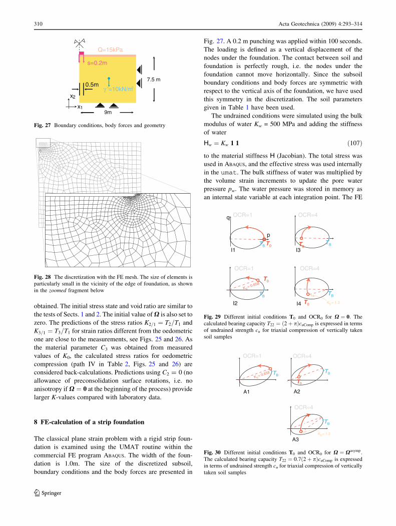
8 FE-calculation of a strip foundation
The classical plane strain problem with a rigid strip foun-
dation is examined using the UMAT routine within the
commercial FE program ABAQUS. The width of the foun-
dation is 1.0m. The size of the discretized subsoil,
boundary conditions and the body forces are presented in
Fig. 27. A 0.2 m punching was applied within 100 seconds.
The loading is defined as a vertical displacement of the
nodes under the foundation. The contact between soil and
foundation is perfectly rough, i.e. the nodes under the
foundation cannot move horizontally. Since the subsoil
boundary conditions and body forces are symmetric with
respect to the vertical axis of the foundation, we have used
this symmetry in the discretization. The soil parameters
given in Table 1 have been used.
The undrained conditions were simulated using the bulk
modulus of water Kw = 500 MPa and adding the stiffness
of water
Hw ¼ Kw 1 1 ð107Þ
to the material stiffness H (Jacobian). The total stress was
used in ABAQUS, and the effective stress was used internally
in the umat. The bulk stiffness of water was multiplied by
the volume strain increments to update the pore water
pressure pw. The water pressure was stored in memory as
an internal state variable at each integration point. The FE
9m
7.5 m0.5m
s=0.2m
Q=15kPa
γ '=10kN/m3
x1
x2
Fig. 27 Boundary conditions, body forces and geometry
Fig. 28 The discretization with the FE mesh. The size of elements is
particularly small in the vicinity of the edge of foundation, as shown
in the zoomed fragment below K = 0.6580
TBT0
TB
T0
p
q
TB T0
TB
T0
OCR=1
OCR=1
OCR=4
OCR=4
K = 1.30
3I1I
I2 I4
Fig. 29 Different initial conditions T0 and OCR0 for X ¼ 0: The
calculated bearing capacity T22 ¼ ð2þ pÞcuComp is expressed in terms
of undrained strength cu for triaxial compression of vertically taken
soil samples
TB
T0
TB
K = 1.30
K = 0.6580
TB
OCR=1 OCR=4
OCR=4
A1 A2
A3
Fig. 30 Different initial conditions T0 and OCR0 for X ¼ Xasymp:The calculated bearing capacity T22 ¼ 0:7ð2þ pÞcuComp is expressed
in terms of undrained strength cu for triaxial compression of vertically
taken soil samples
310 Acta Geotechnica (2009) 4:293–314
123

mesh is shown in Fig. 28. The CPE4 elements of ABAQUS
have been used. Despite full integration, the volumetric
locking (due to water stiffness or due to isochoric plastic
flow) was eliminated by usage of a special volume strain
operator that provided a constant volumetric strain in all
four Gauss integration points within an element. The
consolidation elements of ABAQUS e.g. CPE4P or CPE8P
were not used.
At first, the geometric nonlinearity (ABAQUS uses
Hughes-Winget algorithm) was used, but due to consider-
able distortion of elements (a 0.2 m punching was applied)
the calculation was slowed down to over 1 h on a con-
ventional PC. In order to enable fast comparisons, the
geometric nonlinearity was switched off and as a result the
0.2 m punching took only a quarter of an hour.
The initial conditions for stress T preconsolidation
pressure pB and anisotropy X were all varied. The vertical
stress component was given by the buoyant unit weight of
soil c0 ¼ 10kN/m3 and additionally increased by an equally
distributed surcharge of 15 kPa, Fig. 27. The horizontal
stress was calculated using the coefficient of earth pressure
at rest K0 = 1 - sinuc, K0 = 1.0, and K0 = 1.3. The
anisotropic structure tensor was either switched off X ¼ 0
or taken in the value X ¼ Xasymp0 which results from uni-
axial vertical deformation along x2, since diag[0, -1, 0] is
used in the model as the direction of sedimentation. The
latter choice corresponds to natural K0 - consolidation. The
preconsolidation pressure pB was calculated multiplying
pB? from Eq. 40 (a function of T and XÞ with OCR = 1 or
with OCR = 4. The combinations of the initial conditions
and the resulting bearing capacities obtained from the FE
calculation are given in Figs. 29, 30 and 31.
In each case, a limit load was reached. The vertical dis-
placement necessary to reach the asymptotic reaction force
under the foundation varied from 0.06 to 0.16 m. It is inter-
esting to observe that the limit load related to the undrained
strength cuComp at the depth of 1m corresponds approxi-
mately to the limit analysis solution T22 ¼ ð2þ pÞcuComp
by Prandtl for the isotropic preconsolidation and to about
77% of this value for the anisotropic preconsolidation.
9 Concluding remarks
The anisotropic visco-hypoplastic model presented here
preserves the merits of the isotropic visco-hypoplasticity
(the description of creep, relaxation and rate dependence),
improves the response to cyclic loading and, of course,
provides an anisotropic enhancement which can be
observed in the response to triaxial (or biaxial) compres-
sion and extension paths after anisotropic K0 consolidation.
The rotation of the preconsolidation surface controlled by
the state variable X provides also a better estimation of K0
during an oedometric compression.
Acknowledgments The financial support from the German Research
Community (DFG-Anisotropy TR 218/4-3) is gratefully acknowledged.
List of symbols
The following symbols are used in this paper
A Auxiliary variable for the intensity of
viscous and hypoplastic strain rates
A, B, C Auxiliary subexpresssions for the
definition of Jacobian H
−0.25
−0.2
−0.15
−0.1
−0.05
0
−0.25
−0.2
−0.15
−0.1
−0.05
0
0 50 100 150 200 250
s =
(m
)
-T22 (kPa)
I1I2
I3 I4
0 50 100 150 200 250
s =
(m
)
-T22 (kPa)
A1 A2 A3
Fig. 31 Load-settlement curves for different initial conditions T0 and TB according to Fig. 29 (left) and Fig. 30 (right)
Acta Geotechnica (2009) 4:293–314 311
123
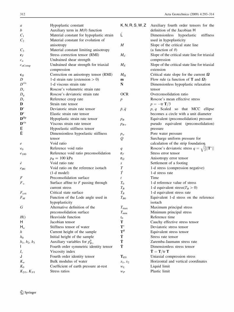
a Hypoplastic constant
b Auxiliary term in M(h) function
C1 Material constant for hypoplastic strain
C2 Material constant for evolution of
anisotropy
C3 Material constant limiting anisotropy
cT Stress correction tensor (RMI)
cu Undrained shear strength
cuComp Undrained shear strength for triaxial
compression
cX Correction on anisotropy tensor (RMI)
D 1-d strain rate (extension [ 0)
Dvis 1-d viscous strain rate
Dv Roscoe’s volumetric strain rate
Dq Roscoe’s deviatoric strain rate
Dr Reference creep rate
D Strain rate tensor
D Deviatoric strain rate tensor
De Elastic strain rate tensor
DHp Hypoplastic strain rate tensor
Dvis Viscous strain rate tensor
E Hypoelastic stiffness tensor
E Dimensionless hypoelastic stiffness
tensor
e Void ratio
e0 Reference void ratio
e100 Reference void ratio preconsolidation
pB = 100 kPa
_e Void ratio rate
eB0 Void ratio on the reference isotach
(1-d model)
F Preconsolidation surface
F? Surface affine to F passing through
current stress
Fcrit Critical state surface
FM Function of the Lode angle used in
hypoplasticity
G Alternative definition of the
preconsolidation surface
H() Heaviside function
H Jacobian tensor
Hw Stiffness tensor of water
h Current height of the sample
h0 Initial height of the sample
h1, h2, h3 Auxiliary variables for p0Bþ
I Fourth order symmetric identity tensor
Iv Viscosity index
J Fourth order identity tensor
Kw Bulk modulus of water
K0 Coefficient of earth pressure at-rest
K2/1, K3/1 Stress ratios
K;N;R;S;W;Z Auxiliary fourth order tensors for the
definition of the Jacobian H
L Dimensionless hypoelastic stiffness
used in hypoplasticity
M Slope of the critical state line
(a function of h)
MC Slope of the critical state line for triaxial
compression
ME Slope of the critical state line for triaxial
extension
MX Critical state slope for the current X
m Flow rule (a function of T and X)
N Dimensionless hypoplastic relaxation
tensor
OCR Overconsolidation ratio
p Roscoe’s mean effective stress
p ¼ tr T=3
p; q p, q Scaled so that MCC ellipse
becomes a circle with a unit diameter
pB Equivalent (preconsolidation) pressure
pB? pseudo equivalent (preconsolidation)
pressure
pw Pore water pressure
Q Surcharge uniform pressure for
calculation of the strip foundation
q Roscoe’s deviatoric stress q ¼ffiffi
32
q
jjTjjrT Stress error tensor
rX Anisotropy error tensor
s Settlement of a footing
T 1-d stress (compression negative)_T 1-d stress rate
t Time
T0 1-d reference value of stress
TB 1-d equivalent stress(TB [ 0)_TB 1-d equivalent stress rate
TB0 Equivalent 1-d stress on the reference
isotach
Tmax Maximum principal stress
Tmin Minimum principal stress
t0 Reference time
T Cauchy effective stress tensor
T Deviatoric stress tensor
TB Equivalent stress tensor_T Stress rate tensorT Zaremba-Jaumann stress rate
T Dimensionless stress tensor
T ¼ T=tr T
TK0 Uniaxial compression stress
x1, x2 Horizontal and vertical coordinates
wL Liquid limit
wP Plastic limit
312 Acta Geotechnica (2009) 4:293–314
123

a strain invariant from [62]
a ¼ffiffiffi
6p
D! D!
: D!
b Auxiliary term in M(h) function
c0 Buoyant unit weight
dij Kroenecker symbol
Dt Increment of t 1-d logarithmic strain
0 1-d reference value of logarithmic strain
h Lode’s angle
k Compression index
j Swelling index
li Coefficients of the general equation of
an ellipse
/ Matsuoka-Nakai’s constant term
/ ¼ 9sin2 uc
1sin2 uc
/(p) Matsuoka-Nakai analogous term for the
alternative preconsolidation surface
/max Constant of the alternative
pre- consolidation surface
uc Critical friction angle
v Positive scalar homogeneity
W Angle between the current stress state
and the isotropic axis
w Coefficient of secondary compression
X Anisotropy tensor
x Anisotropy of the ellipse in p q space
1 Second order identity tensor
References
1. Adachi T, Oka F (1982) Constitutive equations for normally
consolidated clay based on elasto-viscoplasticity. Soil Found
22:57–70
2. Adachi T, Oka F, Hirata T, Hashimoto T, Pradhan TBS, Nagaya
J, Mimura M (1991) Triaxial and torsional hollow cylinder tests
of sensitive natural clay and an elasto-viscoplastic constitutive
model. In: Proceedings of the 10-th ECSMFE, Florence
3. Anandarajah A (2000) On influence of fabric anisotropy on the
stress-strain behaviour of clays. Comp Geotech 27:1–17
4. Axelsson K, Yu Y (1988) Constitutive modelling of swedish fine
grained soils. Mechanical properties and modelling of silty soils.
In: Proceedings of the 2nd nordic geotechnical meeting, Oslo
University, pp 14–18
5. Baligh MM, Whittle A (1987) Soil models and design methods.
In: Geotechnical design: design methods and parameters con-
ference, Politecnico di Torino
6. Banerjee PK, Kumbhojkar A, Yousif NB (1987) A generalized
elasto-plastic model for anisotropically consolidated clays. In:
Desai CS (ed) Constitutive laws for engineering materials: theory
and applications. Elsevier, pp 495–504
7. Banerjee PK, Yousif NB (1986) A plasticity model for the
mechanical behaviour of anisotropically consolidated clay. Int J
Num Anal Meth Geomech 10:521–541
8. Bauer E (2009) Hypoplastic modelling of moisture-sensitive
weathered rockfill materials. Acta Geotech. doi:10.1007/s11440-
009-0099-y
9. Bellotti R, Jamiolkowski M, Lo Presti DCF, O’Neill DA (1996)
Anisotropy of small strain stiffness in Ticino sand. Geotechnique
46(1):115–131
10. Betten J (2008) Creep mechanics. Springer, Berlin
11. Boehler JP, Sawczuk A (1977) On yielding of oriented solids.
Acta Mech 27:185–206
12. Borja RI (1992) Generalized creep and stress relaxation model for
clays. J Geotech Eng Div ASCE 118(11):1765–1786
13. Borja RI, Kavazanjian E (1985) A constitutive model for the
stress–strain-time behaviour of wet clays. Geotechnique
35(3):283–298
14. Burland JB, Georgiannou VN (1991) Small strain stiffness under
generalized stress changes. In: Proceedings of the 10th European
conference soil mechanics and foundation engineering, Florence,
vol 1, pp 41–44
15. Butterfield R (1979) A natural compression law for soils. Geo-
technique 29:469–480
16. Callisto L, Calabresi G (1998) Mechanical behaviour of a natural
soft clay. Geotechnique 48(4):495–513
17. Cormeau I (1975) Numerical stability in quasi-static elasto/visco-
plasticity. Int J Num Meth Eng 9:109–127
18. Dafalias YF (1987) An anisotropic critical state clay plasticity
model. In: Desai CS (ed) Constitutive laws for engineering
materials: theory and applications. Elsevier, pp 513–521
19. Darve F, Butterfield R (1989) Geomaterials: constitutive equa-
tions and modelling. Elsevier, New York
20. Dean ETR (1989) Isotropic transformations models for finite
axial strains events. Technical report 224, Cambridge Geotech-
nical Group
21. Gudehus G (1996) A comprehensive constitutive equation for
granular materials. Soil Found 36(1):1–12
22. Henke S, Grabe J (2008) Numerical investigation of soil plugging
inside open-ended piles with respect to the installation method.
Acta Geotech 3:215–223
23. Houlsby GT, Puzrin AM (2006) Principles of hyperplasticity.
Springer, London
24. Huang WX, Wu W, Sun DA, Sloan S (2006) A simple hypoplastic
model for normally consolidated clay. Acta Geotech 1:15–27
25. Imai G, Yi-Xin Tang (1992) A constitutive equation of one-
dimensional consolidation derived from inter-connected tests.
Soil Found 32(2):83–96
26. Jardine RJ, Symes MJ, Burland JB (1984) The measurement of
soil stiffness in the triaxial apparatus. Geotechnique 34:323–340
27. Kavvadas M (1983) A kinematic hardening constitutive model
for clays. In: Proceedings of 2nd international conference con-
stitutive laws in engineering materials, Tucson, pp 263–270
28. Kutter BL, Sathialingam N (1992) Elastic-viscoplastic modelling
of rate-dependent behaviour of clays. Geotechnique 42(3):427–441
29. Larsson R (1977) Basic behaviour of Scandinavian soft clays.
Technical report 4, Swedish Geotechnical Institute
30. Leoni M, Karstunen M, and Vermeer PA (2008) Anisotropic
creep model for soft soils. Geotechnique 58(3):215–226
31. Leroueil S, Kabbaj M, Tavenas F (1988) Study of the validity of a
XXX model in situ conditions. Soil Found 28(3):13–25
32. Leroueil S, Vaughan PR (1990) The general congruent effects of
structure in natural soils and weak rocks. Geotechnique
40(3):467–488
33. Lewin PI, Burland JB (1970) Stress-probe experiments on satu-
rated normally consolidated clay. Geotechnique 20:38–56
34. Matsuoka H, Nakai T (1977) Stress-strain relationship of soil
based on the SMP, constitutive equations of soils. Speciality
session 9, Japanese society of soil mechanics and foundation
engineering, IX ICSMFE, Tokyo, pp 153–162
35. Masın D, Herle I (2007) Improvement of a hypoplastic model to
predict clay behaviour under undrained conditions. Acta Geotech
2(4):261–268
Acta Geotechnica (2009) 4:293–314 313
123
36. Mesri G, Choi YK (1985) The uniqueness of the end-of-primary
(EOP) void ratio-effective stress relationship. In: Soil mechanics
and foundation engineering, vol 2. Proceedings of the 11th
international conference in San Francisco, USA, pp 587–590
37. Mitchell RJ (1970) On the yielding and mechanical strength of
leda clay. Can Geotech J 7:297–312
38. Mitchell RJ (1972) Some deviations from isotropy in a lightly
overconsolidated clay. Geotechnique 22(3):459–460
39. Molenkamp F, Van Ommen A (1986) Initial state for anisotropic
elasto-plastic model. In: 2nd International symposium on
numerical models in geomechanics, Ghent
40. Mroz Z (1966) On forms of constitutive laws for elastic-plastic
solids. Archiwum Mechaniki Stosowanej
41. Mroz Z, Niemunis A (1987) On the description of deformation
anisotropy of materials. In: Boehler JP (ed) Yielding, damage and
failure of anisotropic solids. Proceedings of IUTAM symposium
in Grenoble, France, pp 171–186
42. Niemunis A (2003) Extended hypoplastic models for soils,
Habilitation, monografia 34, Ruhr-University Bochum
43. Niemunis A, Cudny M (1998) On hyperplasticity for clays.
Comput Geotech 23:221–236
44. Niemunis A, Herle I (1997) Hypoplastic model for cohesionless
soils with elastic strain range. Mech Cohes Frict Mater 2:279–299
45. Niemunis A, Krieg S(1996) Viscous behaviour of soil under
oedometric conditions. Can Geotech J 33(1):159–168
46. Norton F (1929) The creep of steel at high temperatures. Mc
Graw Hill, NY
47. Oka F, Adachi T, Okano Y (1986) Two-dimensional consolida-
tion analysis using an elasto-viscoplastic constitutive equation.
Int J Num Anal Meth Geomech 10:1–16
48. Oka F, Leroueil S, Tavenas F (1989) A constitutive model for
natural soft clay with strain softening. Soil Found 29:54–66
49. Olszak W, Perzyna P (1966) The constitutive equations of the flow
theory for a nonstationary yield condition. In: Applied mechanics.
Proceedings of the 11th international congress, pp 545–553
50. Reyes DK, Rodriguez-Marek A, Lizcano A (2009) A hypoplastic
model for site response analysis. Soil Dyn Earthq Eng 29(1):173–
184
51. Rondon HA, Wichtmann T, Triantafyllidis T, Lizcano A (2007)
Hypoplastic material constants for a well-graded granular mate-
rial for base and subbase layers of flexible pavements. Acta
Geotech 2(2):113–126
52. Salciarini D, Tamagnini C (2009) A hypoplastic macroelement
model for shallow foundations under monotonic and cyclic loads.
Acta Geotech 4(3):163–176
53. Schwer L (1994) A viscoplastic augmentation of the smooth cap
model. In: Siriwardane HJ, Zaman MM (eds) Computer meth-
ods and advances in geomechanics, Balkema, Rotterdam,
pp 671–676
54. Sekiguchi H (1985) Constitutive laws of soils. Macrometric
approaches—static-intrinsically time dependent. In: Discussion
session. Proceedings of the 11th ICSMFE, San Francisco, USA
55. Simpson B (1992) Retaining structures: displacement and design.
Geotechnique 42(4):541–576
56. Stallebrass E (1990) Modelling of the effect of recent stress
history on the deformation of overconsolidated soils. PhD thesis,
The City University
57. Sturm H (2004) Modelling of biaxial tests on remoulded saturated
clay with a visco-hzpoplastic constitutive law, 2004. Diplomar-
beit, Institut fur Boden und Felsmechanik, Universitat Karlsruhe
58. Sturm H (2009) Numerical investigation of the stabilisation
behaviour of shallow foundations under alternate loading. Acta
Geotech. doi: 10.1007/s11440-09-0102-7
59. Suklje L (1969) Rheological aspects of soil mechanics. Wiley,
London
60. Weifner T, Kolymbas D (2007) A hypoplastic model for clay and
sand. Acta Geotech 2(2):103–112
61. Tejchman J, Bauer E, Tantono SF (2007) Influence of initial
density of cohesionless soil on evolution of passive earth pres-
sure. Acta Geotech 2(1):53–63
62. Tejchman J, Gorski J (2009) Finite element study of patterns of
shear zones in granular bodies during plane strain compression.
Acta Geotech. doi: 10.1007/s11440-009-0103-6
63. Topolnicki M (1987) Observed stress–strain behaviour of re-
moulded saturated clay and examination of two constitutive
models Heft 107, Institut fur Boden und Felsmechanik, Univer-
sitat Karlsruhe
64. Whittle AJ, Kavvadas MJ (1994) Formulation of mit-e3 consti-
tutive model for overconsolidated clays. J Geotech Eng Div
ASCE 120(1):173–198
65. Wolffersdorff PAv (1996) A hypoplastic relation for granular
materials with a predefined limit state surface. Mech Cohes Frict
Mater 1:251–271
66. Wolfram S (2004) The Mathematica Book, 5th edn. Wolfram
Media, Inc, Champaign
67. Yong RN, Mohamed AO (1988) Performance prediction of
anisotropic clays under loading. 114(3)
68. Zienkiewicz OC, Cormeau IC (1974) Visco-plasticity—plasticity
and creep in elastic solids—a unified numerical solution
approach. Int J Num Meth Eng 8:821–845
314 Acta Geotechnica (2009) 4:293–314
123