announcement ams conversation on non-academic employment: friday, january 15, 9:30am to 11am,...
TRANSCRIPT

AnnouncementAnnouncement
• AMS Conversation on Non-Academic Employment: Friday, January 15, 9:30am to 11am, Moscone West Room 2008
• Also you can drop by Booth No. 812 on Friday, January 15, 6-7pm., to talk to the people there about the Certificate in Quantitative Finance (CQF), a 6-month, part-time course for those interested in derivatives, development, quantitative trading or risk management.

Structural Equation Modeling Structural Equation Modeling with New Development for with New Development for
Mixed DesignsMixed DesignsPlus Introductions toPlus Introductions to
Time Series Modeling, Bootstrap Time Series Modeling, Bootstrap Resampling, & Partial Correlation Resampling, & Partial Correlation
Network Analysis (PCNA)Network Analysis (PCNA)
Kathryn SharpeKathryn Sharpe
Wei ZhuWei Zhu

3
OutlineOutlinePart I: SEM & Introduction to Time Series
Models• A brief introduction to SEM with an eating
disorder example• A fMRI time series study + AR and MV
models in SEM notation• SEM for Mixed Designs with a PET study
example
Part II: PCNA and Bootstrap Resampling
1. Partial Correlation Network Analysis
2. Bootstrap Resampling
Part I: SEM & Introduction to Time Part I: SEM & Introduction to Time Series ModelsSeries Models
1. A brief introduction to SEM with an eating disorder example
5
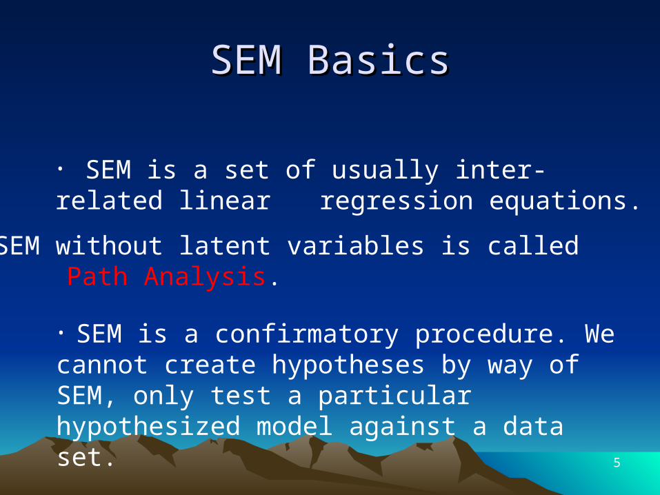
SEM BasicsSEM Basics
• SEM without latent variables is called Path Analysis.
• SEM is a confirmatory procedure. We cannot create hypotheses by way of SEM, only test a particular hypothesized model against a data set.
• SEM is a set of usually inter-related linear regression equations.

6
Assumptions of SEMAssumptions of SEM
Large samples:
The variables follow a multivariate normal distribution.
SEM researchers suggest a sample size of at least ten times the number of parameters we will be estimating.
Now, we present a simple example of SEM.
7
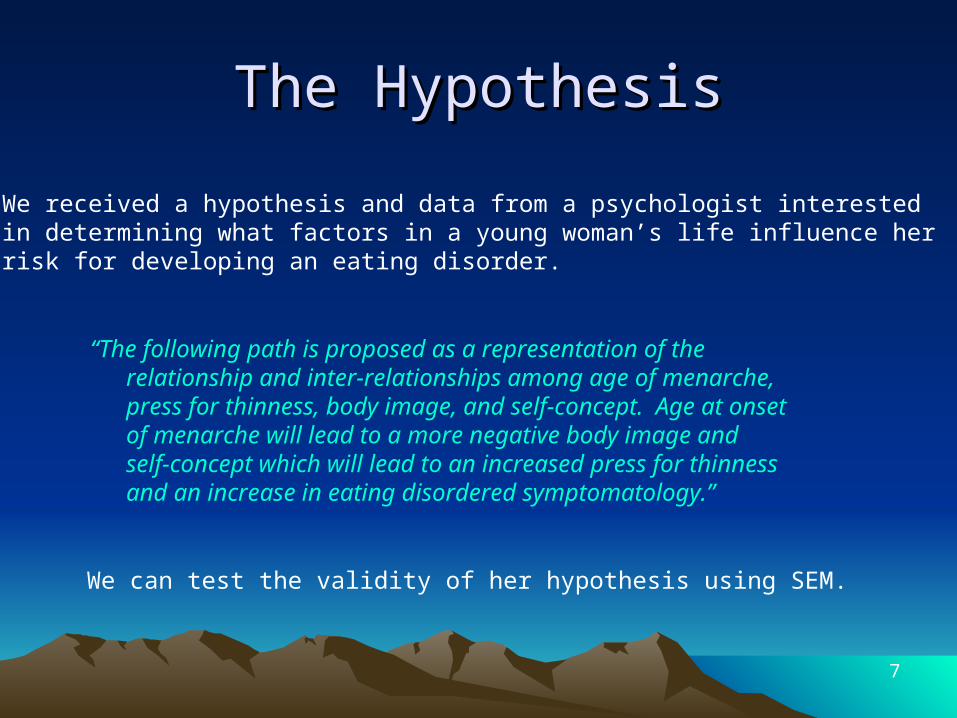
The HypothesisThe Hypothesis
We received a hypothesis and data from a psychologist interested in determining what factors in a young woman’s life influence her risk for developing an eating disorder.
“The following path is proposed as a representation of the relationship and inter-relationships among age of menarche, press for thinness, body image, and self-concept. Age at onsetof menarche will lead to a more negative body image andself-concept which will lead to an increased press for thinnessand an increase in eating disordered symptomatology.”
We can test the validity of her hypothesis using SEM.
8
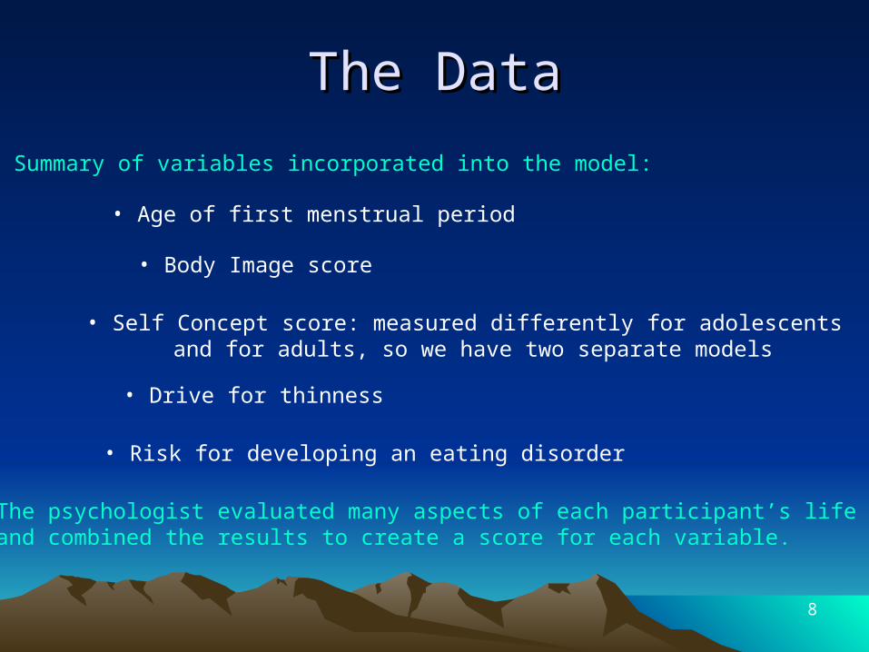
The DataThe Data
• Age of first menstrual period
• Body Image score
• Self Concept score: measured differently for adolescents and for adults, so we have two separate models
• Drive for thinness
• Risk for developing an eating disorder
The psychologist evaluated many aspects of each participant’s lifeand combined the results to create a score for each variable.
Summary of variables incorporated into the model:

9
Listwise/Pairwise DeletionListwise/Pairwise Deletion
There are several ways a researcher can deal with missing data values. Two of them are listed here. In both cases, we assume that any missing data is missing completely at random. If muchdata is lost in deletion, imputation should be considered.
Listwise Deletion:
Pairwise Deletion:
We delete a subject from the study if any of its measurement values are missing.
We omit those subjects from a particular calculation who do not have the corresponding measurement value. The subjects are present in any calculation for which their value exists.
In our study, we use listwise deletion to delete those subjects who do not have the age of first menstrual period variable. We lose less than 10% of our data in deletion.
What do we do when we have missing measurements?
10
Creating Two ModelsCreating Two Models
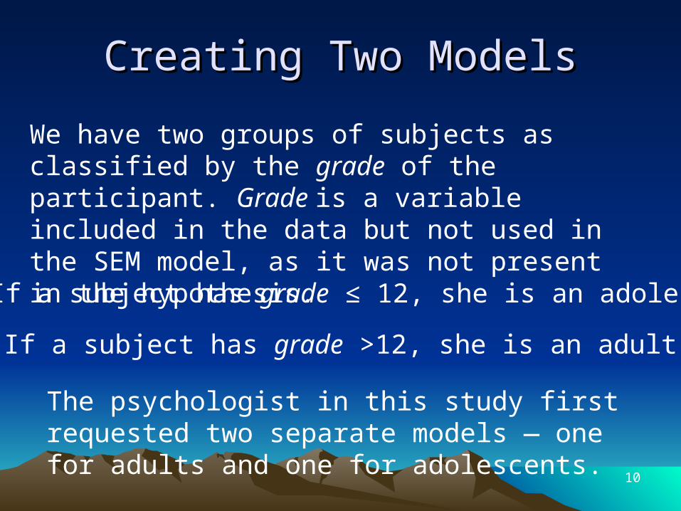
We have two groups of subjects as classified by the grade of the participant. Grade is a variable included in the data but not used in the SEM model, as it was not present in the hypothesis.
The psychologist in this study first requested two separate models — one for adults and one for adolescents.
• If a subject has grade ≤ 12, she is an adolescent.
• If a subject has grade >12, she is an adult.

11
Path DiagramsPath Diagrams
Age of Menstruation
(AM)
Body Image(BI)
AdolescentSelf Worth (SW)
Drive for Thinness (DT)
Risk for Disorder (RD)
Drive for Thinness (DT)
AdultSelf Worth (SW)
Age of Menstruation
(AM)
Directional Arrows indicate cause and effect
Body Image(BI)
Risk for Disorder (RD)

12
The EquationsThe Equations
Because there are no latent variables, we can write basic regression equations for each variable. Our system is as follows:
SW AM BI 3 4 2
DT B I SW 5 6 3
RD DT 7 4
B I AM SW 1 2 1

13
SEM ProgramsSEM Programs
For this example, we will use PROC CALIS. It takes our linear equations (previous slide) and estimates the parameters for the model. Then it evaluates the goodness of fit of the model.
• PROC CALIS (and PROC TCALIS) in SAS
• LISREL
• EQS (Peter Bentler)
• AMOS
The most popular software packages for SEM are:
14
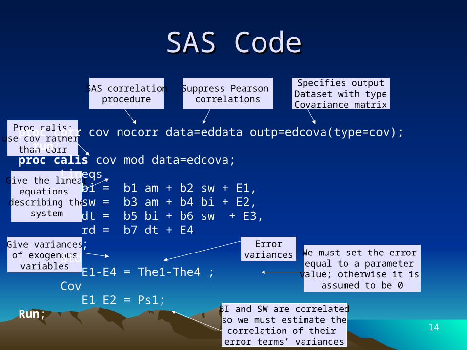
SAS CodeSAS Code
Give the linearequations
describing thesystem
Suppress Pearson correlations
Proc calis:use cov rather
than corr
SAS correlationprocedure
Give variancesof exogenous
variables
Errorvariances
Specifies outputDataset with typeCovariance matrix
proc corr cov nocorr data=eddata outp=edcova(type=cov); run;proc calis cov mod data=edcova; Lineqs bi = b1 am + b2 sw + E1, sw = b3 am + b4 bi + E2, dt = b5 bi + b6 sw + E3, rd = b7 dt + E4 ; Std E1-E4 = The1-The4 ; Cov E1 E2 = Ps1; Run;
We must set the error equal to a parameter value; otherwise it is
assumed to be 0
BI and SW are correlatedso we must estimate the
correlation of their error terms’ variances
15
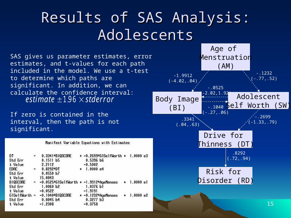
Results of SAS Analysis: AdolescentsResults of SAS Analysis: AdolescentsAge of
Menstruation(AM)
Body Image(BI)
AdolescentSelf Worth (SW)
Drive for Thinness (DT)
Risk for Disorder (RD)
SAS gives us parameter estimates, error estimates, and t-values for each path included in the model. We use a t-test to determine which paths are significant. In addition, we can calculate the confidence interval:
-1.9912(-4.02,.04)
-.1232(-.77,.52)
-.2699(-1.33,.79)
.8292(.72,.94)
-.1040(-.27,.06)
-.0525(-2.02,1.92)
.3341(.04,.63)
If zero is contained in the interval, then the path is not significant.
estim a te stderror 1 9 6.

16
Results of SAS Analysis: AdultsResults of SAS Analysis: Adults
Age of Menstruation
(AM)
Body Image(BI)
AdolescentSelf Worth (SW)
Drive for Thinness (DT)
Risk for Disorder (RD)
-.4157(-2.89,2.06)
.2262(-.46,.99)
-.2998(-2.19,1.59)
-.1289(-.33,.07) .4255
(-.43,1.28).8285(.55,1.11)
.8960(.77,1.03)
Here again, we use a t-test and/or the confidence intervals to evaluate which paths are significant.
SAS Output:

17
Goodness of FitGoodness of FitAfter reporting the parameter estimates, SAS reports many different measures of fit so we can evaluate it in any way we choose. The more measures we use to evaluate our model, the better.
A good fit does not necessarilymean a perfect model. We canstill have unnecessary variablesor be missing important ones.
By convention, a model is “good” if:
• GFI > .90/.95,
• Small Chi-Square value,large p-value,
• RMSEA Estimate should be close to zero.
Adolescent:
Adult:

Part I: SEM & Introduction to Time Part I: SEM & Introduction to Time Series ModelsSeries Models
2. A fMRI time series study + AR and MV models in SEM notation

19
SEM for Brain Functional SEM for Brain Functional Pathway AnalysisPathway Analysis
SEM can be utilized to study brain functional pathways based on brain image studies including the positron emission tomography (PET), & the functional magnetic resonance imaging (fMRI) studies.
Each PET scan generates only one 3D image, while each fMRI scan generates a time series of images tabulating continuous brain functional activities.
20
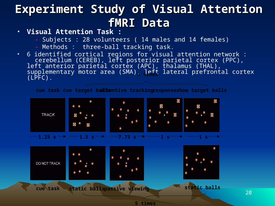
Experiment Study of Visual Attention fMRI Experiment Study of Visual Attention fMRI DataData
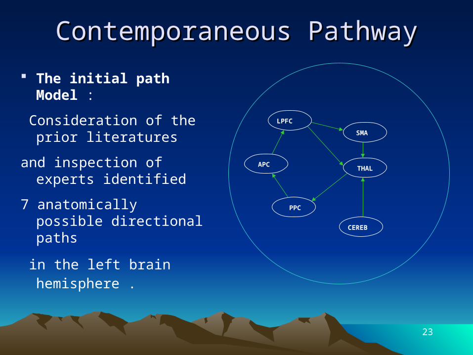
• Visual Attention Task : - Subjects : 28 volunteers ( 14 males and 14 females) - Methods : three-ball tracking task.• 6 identified cortical regions for visual attention network : cerebellum (CEREB), left posterior parietal cortex (PPC), left anterior parietal cortex
(APC), thalamus (THAL), supplementary motor area (SMA), left lateral prefrontal cortex (LPFC).
cue task
cue task
1.25 s
static balls
cue target balls
1.5 s
passive viewing
attentive tracking
7.75 s 1 s
response
static balls
1 s
show target balls
5 times
5 times

21
Study DesignStudy Design
Data : fMRI data at coordinates corresponding the 6 regions from each individual data set.
Extracting the activation (onset) conditions. Hemodynamic delay : The first two time points ( 2 TR, 6 sec) at
each onset
ACTIVE PASSIVE ACTIVEACTIVE PASSIVEPASSIVE
ON ONONOFF OFFOFF
60 sec 60 sec60 sec60 sec 60 sec60 sec
20 Images 20 Images 20 Images20 Images 20 Images20 Images

22
Structure of fMRI DataStructure of fMRI Data
23
Contemporaneous PathwayContemporaneous Pathway
The initial path Model :
Consideration of the prior literatures
and inspection of experts identified
7 anatomically possible directional paths
in the left brain hemisphere .
LPFC
PPC
SMA
THALAPC
CEREB

24
Longitudinal Pathways Longitudinal Pathways Modeled by MAR(1) Modeled by MAR(1)
time t-1 time t
1y
2y
6y
3y
4y
5y
1y
2y
6y
3y
4y
5y

25
- The original model with the longitudinal relations and the contemporaneous relations in the same path diagram.
- This model is used as the original model through all approaches to visual attention fMRI data.
tt-1
tt-1
tt-1
tt-1
t
t-1
t
t-1
CEREB
THAL
SMA
PPC
APC
LPFC
Unified SEM of Visual Attention fMRI data
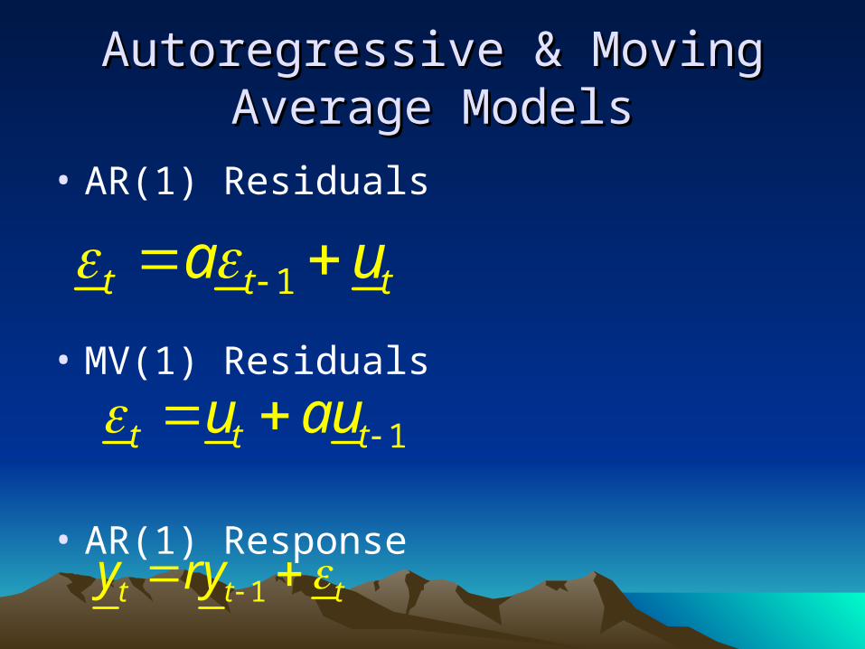
Autoregressive & Moving Average Autoregressive & Moving Average ModelsModels
• AR(1) Residuals
• MV(1) Residuals
• AR(1) Response
1t t ta u
1t t ty ry
1t t tu au

Autoregressive & Moving Average Autoregressive & Moving Average Models in SEM NotationsModels in SEM Notations
AR(1) Residuals, MV(1) Residuals, AR(1) Response
1t t ta u 1t t tu au 1t t ty ry
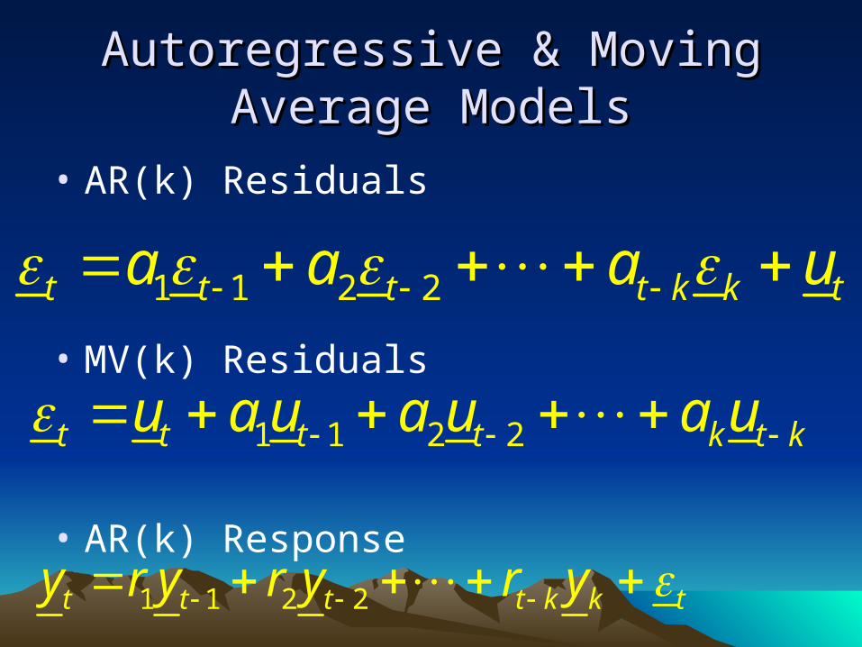
Autoregressive & Moving Average Autoregressive & Moving Average ModelsModels
• AR(k) Residuals
• MV(k) Residuals
• AR(k) Response
1 1 2 2t t t t k k ta a a u
1 1 2 2t t t t k k ty r y r y r y
1 1 2 2t t t t k t ku a u a u a u

Monthly Sales and Forecast
0
200
400
600
800
1000
1200
1400
1600
1800
2000
1 2 3 4 5 6 7 8 9 10 11 12 13 14 15 16 17 18 19 20 21 22 23 24 25
Month
Sal
es (
$100
0)
Monthly Sales
Forecast
Monthly Sales and Forecast
0
200
400
600
800
1000
1200
1400
1600
1800
2000
1 2 3 4 5 6 7 8 9 10 11 12 13 14 15 16 17 18 19 20 21 22 23 24 25
Month
Sal
es (
$100
0)
Monthly Sales
Forecast
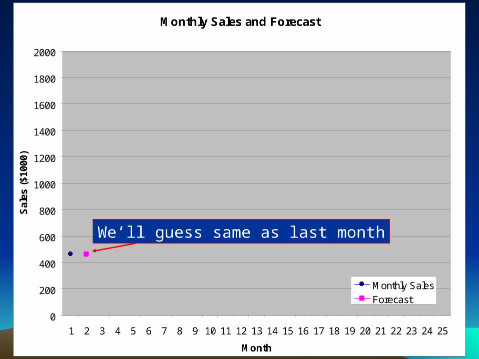
We’ll guess same as last month

Monthly Sales and Forecast
0
200
400
600
800
1000
1200
1400
1600
1800
2000
1 2 3 4 5 6 7 8 9 10 11 12 13 14 15 16 17 18 19 20 21 22 23 24 25
Month
Sal
es (
$100
0)
Monthly Sales
Forecast

Monthly Sales and Forecast
0
200
400
600
800
1000
1200
1400
1600
1800
2000
1 2 3 4 5 6 7 8 9 10 11 12 13 14 15 16 17 18 19 20 21 22 23 24 25
Month
Sal
es (
$100
0)
Monthly Sales
Forecast
We’ll guess same as last monthplus a little more for a possible trend

Monthly Sales and Forecast
0
200
400
600
800
1000
1200
1400
1600
1800
2000
1 2 3 4 5 6 7 8 9 10 11 12 13 14 15 16 17 18 19 20 21 22 23 24 25
Month
Sal
es (
$100
0)
Monthly Sales
Forecast
This is easy, who needs forecasting

Monthly Sales and Forecast
0
200
400
600
800
1000
1200
1400
1600
1800
2000
1 2 3 4 5 6 7 8 9 10 11 12 13 14 15 16 17 18 19 20 21 22 23 24 25
Month
Sal
es (
$100
0)
Monthly Sales
Forecast
Continue with our successful method: guess the same as last month plus a little more for a possible trend

Monthly Sales and Forecast
0
200
400
600
800
1000
1200
1400
1600
1800
2000
1 2 3 4 5 6 7 8 9 10 11 12 13 14 15 16 17 18 19 20 21 22 23 24 25
Month
Sal
es (
$100
0)
Monthly Sales
Forecast
Monthly Sales and Forecast
0
200
400
600
800
1000
1200
1400
1600
1800
2000
1 2 3 4 5 6 7 8 9 10 11 12 13 14 15 16 17 18 19 20 21 22 23 24 25
Month
Sal
es (
$100
0)
Monthly Sales
Forecast
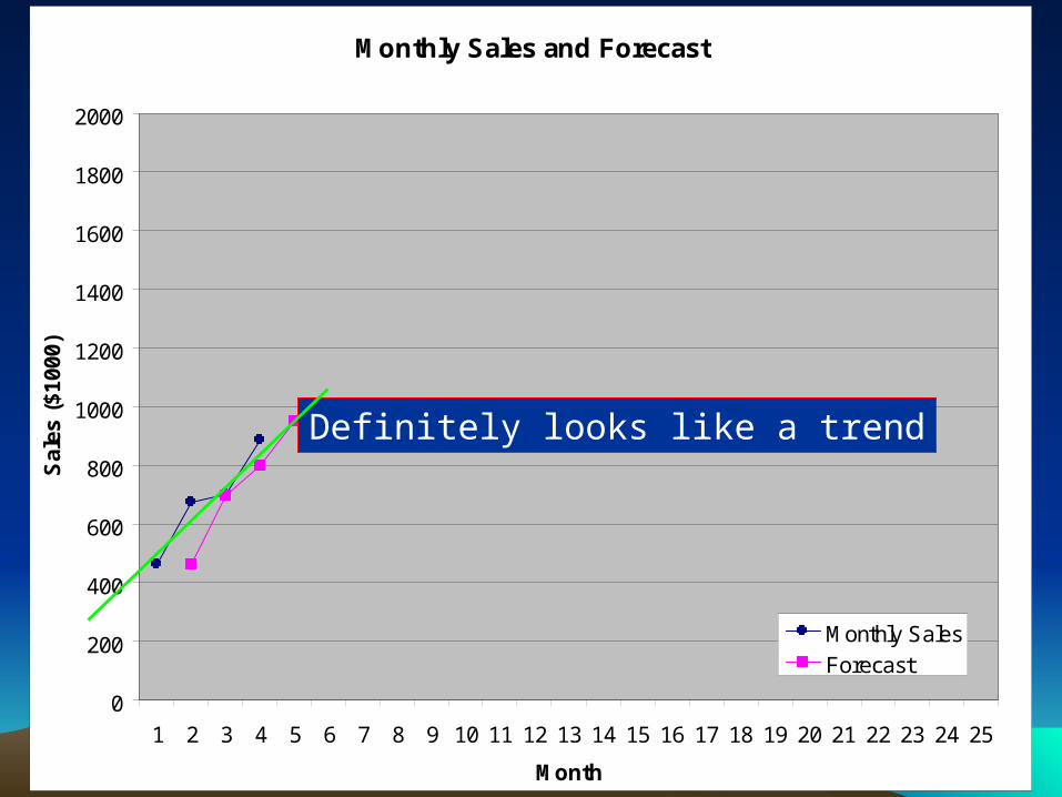
Definitely looks like a trend

Monthly Sales and Forecast
0
200
400
600
800
1000
1200
1400
1600
1800
2000
1 2 3 4 5 6 7 8 9 10 11 12 13 14 15 16 17 18 19 20 21 22 23 24 25
Month
Sal
es (
$100
0)
Monthly Sales
Forecast

Monthly Sales and Forecast
0
200
400
600
800
1000
1200
1400
1600
1800
2000
1 2 3 4 5 6 7 8 9 10 11 12 13 14 15 16 17 18 19 20 21 22 23 24 25
Month
Sal
es (
$100
0)
Monthly Sales
Forecast
Trend might be a tad steeper than I thought

Monthly Sales and Forecast
0
200
400
600
800
1000
1200
1400
1600
1800
2000
1 2 3 4 5 6 7 8 9 10 11 12 13 14 15 16 17 18 19 20 21 22 23 24 25
Month
Sal
es (
$100
0)
Monthly Sales
Forecast
Opps

Monthly Sales and Forecast
0
200
400
600
800
1000
1200
1400
1600
1800
2000
1 2 3 4 5 6 7 8 9 10 11 12 13 14 15 16 17 18 19 20 21 22 23 24 25
Month
Sal
es (
$100
0)
Monthly Sales
Forecast
Momentary deviation, trend will continue
Monthly Sales and Forecast
0
200
400
600
800
1000
1200
1400
1600
1800
2000
1 2 3 4 5 6 7 8 9 10 11 12 13 14 15 16 17 18 19 20 21 22 23 24 25
Month
Sal
es (
$100
0)
Monthly Sales
Forecast
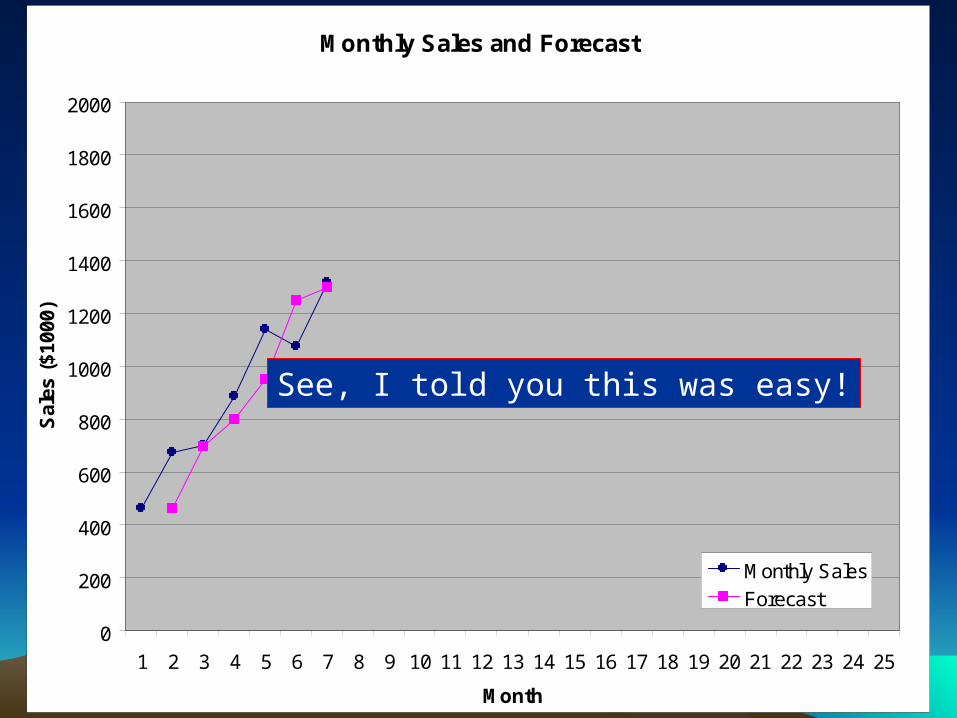
See, I told you this was easy!

Monthly Sales and Forecast
0
200
400
600
800
1000
1200
1400
1600
1800
2000
1 2 3 4 5 6 7 8 9 10 11 12 13 14 15 16 17 18 19 20 21 22 23 24 25
Month
Sal
es (
$100
0)
Monthly Sales
Forecast
Trend will continue

Monthly Sales and Forecast
0
200
400
600
800
1000
1200
1400
1600
1800
2000
1 2 3 4 5 6 7 8 9 10 11 12 13 14 15 16 17 18 19 20 21 22 23 24 25
Month
Sal
es (
$100
0)
Monthly Sales
Forecast
Opps, another momentary fluctuation:
Monthly Sales and Forecast
0
200
400
600
800
1000
1200
1400
1600
1800
2000
1 2 3 4 5 6 7 8 9 10 11 12 13 14 15 16 17 18 19 20 21 22 23 24 25
Month
Sal
es (
$100
0)
Monthly Sales
Forecast
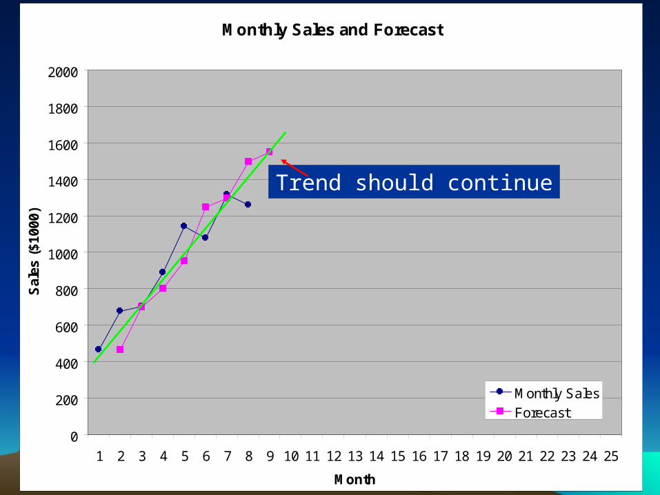
Trend should continue

Monthly Sales and Forecast
0
200
400
600
800
1000
1200
1400
1600
1800
2000
1 2 3 4 5 6 7 8 9 10 11 12 13 14 15 16 17 18 19 20 21 22 23 24 25
Month
Sal
es (
$100
0)
Monthly Sales
Forecast
Oh oh!

Monthly Sales and Forecast
0
200
400
600
800
1000
1200
1400
1600
1800
2000
1 2 3 4 5 6 7 8 9 10 11 12 13 14 15 16 17 18 19 20 21 22 23 24 25
Month
Sal
es (
$100
0)
Monthly Sales
Forecast
Sales has leveled off:Lets average last few points

Monthly Sales and Forecast
0
200
400
600
800
1000
1200
1400
1600
1800
2000
1 2 3 4 5 6 7 8 9 10 11 12 13 14 15 16 17 18 19 20 21 22 23 24 25
Month
Sal
es (
$100
0)
Monthly Sales
Forecast
Oh oh, maybe things are going down hill

Monthly Sales and Forecast
0
200
400
600
800
1000
1200
1400
1600
1800
2000
1 2 3 4 5 6 7 8 9 10 11 12 13 14 15 16 17 18 19 20 21 22 23 24 25
Month
Sal
es (
$100
0)
Monthly Sales
Forecast
Let’s be conservative andAssume a negative trend
Monthly Sales and Forecast
0
200
400
600
800
1000
1200
1400
1600
1800
2000
1 2 3 4 5 6 7 8 9 10 11 12 13 14 15 16 17 18 19 20 21 22 23 24 25
Month
Sal
es (
$100
0)
Monthly Sales
Forecast
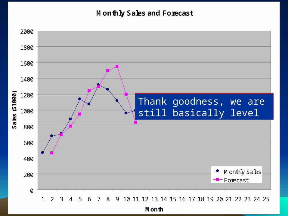
Thank goodness, we are still basically level

Monthly Sales and Forecast
0
200
400
600
800
1000
1200
1400
1600
1800
2000
1 2 3 4 5 6 7 8 9 10 11 12 13 14 15 16 17 18 19 20 21 22 23 24 25
Month
Sal
es (
$100
0)
Monthly Sales
Forecast
We’ll guess same as last month
Monthly Sales and Forecast
0
200
400
600
800
1000
1200
1400
1600
1800
2000
1 2 3 4 5 6 7 8 9 10 11 12 13 14 15 16 17 18 19 20 21 22 23 24 25
Month
Sal
es (
$100
0)
Monthly Sales
Forecast
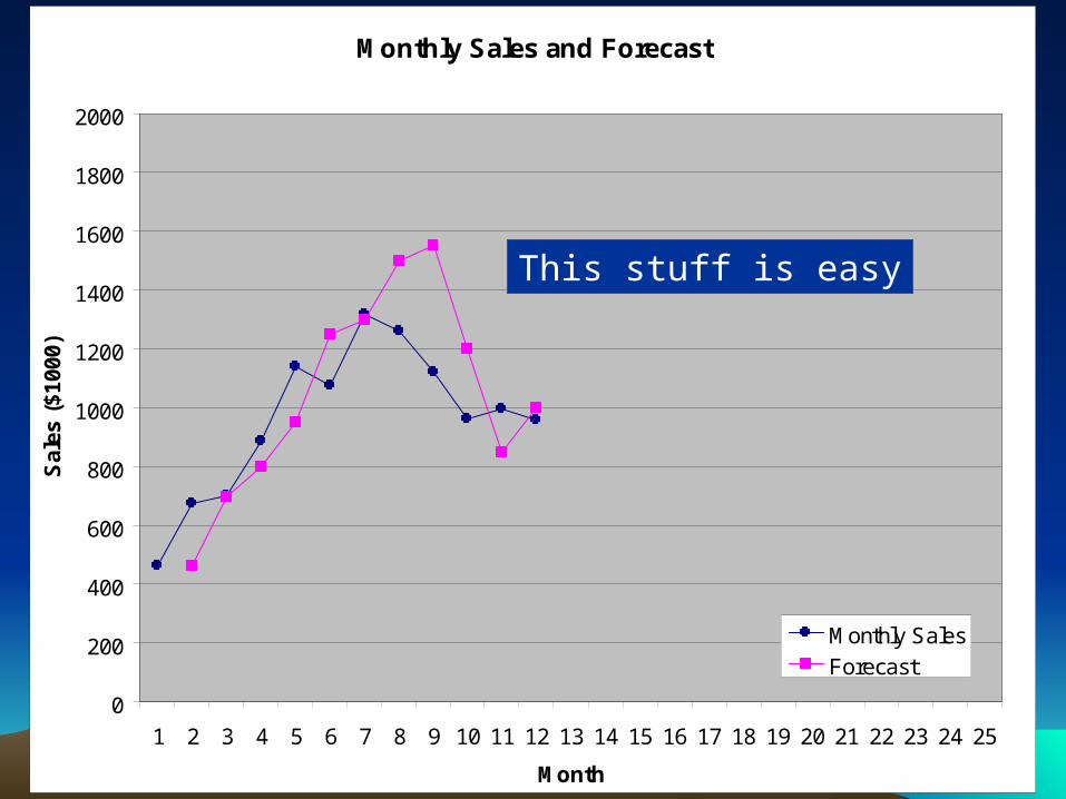
This stuff is easy

Monthly Sales and Forecast
0
200
400
600
800
1000
1200
1400
1600
1800
2000
1 2 3 4 5 6 7 8 9 10 11 12 13 14 15 16 17 18 19 20 21 22 23 24 25
Month
Sal
es (
$100
0)
Monthly Sales
Forecast
We have for sure leveled off
Monthly Sales and Forecast
0
200
400
600
800
1000
1200
1400
1600
1800
2000
1 2 3 4 5 6 7 8 9 10 11 12 13 14 15 16 17 18 19 20 21 22 23 24 25
Month
Sal
es (
$100
0)
Monthly Sales
Forecast
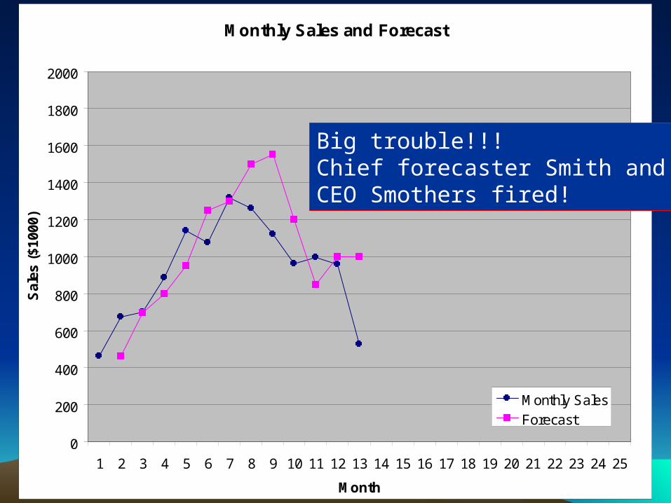
Big trouble!!!Chief forecaster Smith andCEO Smothers fired!

Monthly Sales and Forecast
0
200
400
600
800
1000
1200
1400
1600
1800
2000
1 2 3 4 5 6 7 8 9 10 11 12 13 14 15 16 17 18 19 20 21 22 23 24 25
Month
Sal
es (
$100
0)
Monthly Sales
Forecast
New chief forecaster pointsout the obvious trend

Monthly Sales and Forecast
0
200
400
600
800
1000
1200
1400
1600
1800
2000
1 2 3 4 5 6 7 8 9 10 11 12 13 14 15 16 17 18 19 20 21 22 23 24 25
Month
Sal
es (
$100
0)
Monthly Sales
Forecast
Remarkable turnaround in sales.New CEO Smithers given credit

Monthly Sales and Forecast
0
200
400
600
800
1000
1200
1400
1600
1800
2000
1 2 3 4 5 6 7 8 9 10 11 12 13 14 15 16 17 18 19 20 21 22 23 24 25
Month
Sal
es (
$100
0)
Monthly Sales
Forecast
Still looks like a trend to me
Monthly Sales and Forecast
0
200
400
600
800
1000
1200
1400
1600
1800
2000
1 2 3 4 5 6 7 8 9 10 11 12 13 14 15 16 17 18 19 20 21 22 23 24 25
Month
Sal
es (
$100
0)
Monthly Sales
Forecast
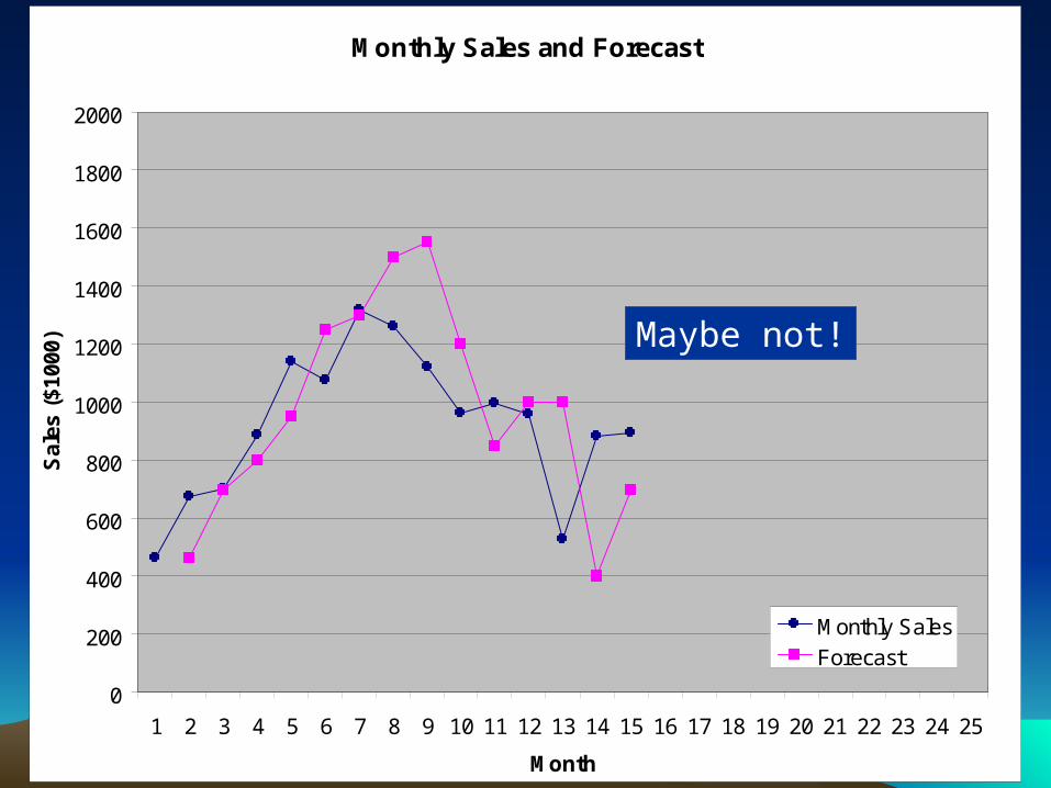
Maybe not!

Monthly Sales and Forecast
0
200
400
600
800
1000
1200
1400
1600
1800
2000
1 2 3 4 5 6 7 8 9 10 11 12 13 14 15 16 17 18 19 20 21 22 23 24 25
Month
Sal
es (
$100
0)
Monthly Sales
Forecast
Level except for anomaly
Monthly Sales and Forecast
0
200
400
600
800
1000
1200
1400
1600
1800
2000
1 2 3 4 5 6 7 8 9 10 11 12 13 14 15 16 17 18 19 20 21 22 23 24 25
Month
Sal
es (
$100
0)
Monthly Sales
Forecast
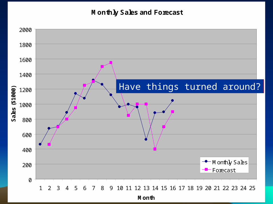
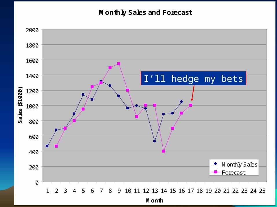
Have things turned around?
Monthly Sales and Forecast
0
200
400
600
800
1000
1200
1400
1600
1800
2000
1 2 3 4 5 6 7 8 9 10 11 12 13 14 15 16 17 18 19 20 21 22 23 24 25
Month
Sal
es (
$100
0)
Monthly Sales
Forecast
I’ll hedge my bets
Monthly Sales and Forecast
0
200
400
600
800
1000
1200
1400
1600
1800
2000
1 2 3 4 5 6 7 8 9 10 11 12 13 14 15 16 17 18 19 20 21 22 23 24 25
Month
Sal
es (
$100
0)
Monthly Sales
Forecast
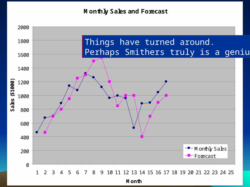
Things have turned around.Perhaps Smithers truly is a genius

Monthly Sales and Forecast
0
200
400
600
800
1000
1200
1400
1600
1800
2000
1 2 3 4 5 6 7 8 9 10 11 12 13 14 15 16 17 18 19 20 21 22 23 24 25
Month
Sal
es (
$100
0)
Monthly Sales
Forecast
Trend up!
Monthly Sales and Forecast
0
200
400
600
800
1000
1200
1400
1600
1800
2000
1 2 3 4 5 6 7 8 9 10 11 12 13 14 15 16 17 18 19 20 21 22 23 24 25
Month
Sal
es (
$100
0)
Monthly Sales
Forecast
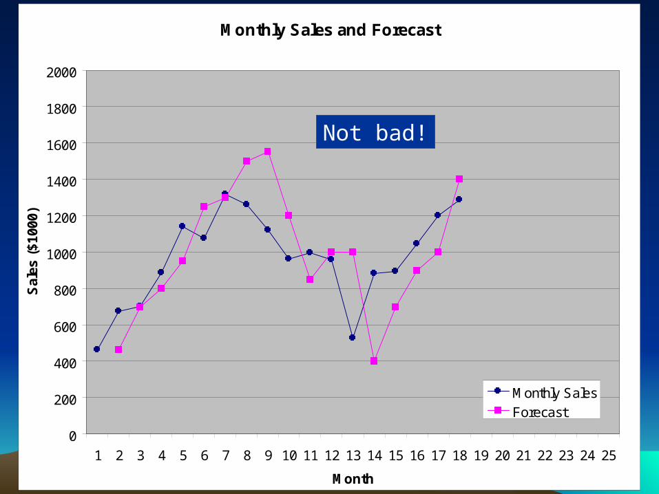
Not bad!

Monthly Sales and Forecast
0
200
400
600
800
1000
1200
1400
1600
1800
2000
1 2 3 4 5 6 7 8 9 10 11 12 13 14 15 16 17 18 19 20 21 22 23 24 25
Month
Sal
es (
$100
0)
Monthly Sales
Forecast
Revise trend a tad

Monthly Sales and Forecast
0
200
400
600
800
1000
1200
1400
1600
1800
2000
1 2 3 4 5 6 7 8 9 10 11 12 13 14 15 16 17 18 19 20 21 22 23 24 25
Month
Sal
es (
$100
0)
Monthly Sales
Forecast
Smithers makes cover of Fortune
Smothers
Smithers

Monthly Sales and Forecast
0
200
400
600
800
1000
1200
1400
1600
1800
2000
1 2 3 4 5 6 7 8 9 10 11 12 13 14 15 16 17 18 19 20 21 22 23 24 25
Month
Sal
es (
$100
0)
Monthly Sales
Forecast
This is easy!!

Monthly Sales and Forecast
0
200
400
600
800
1000
1200
1400
1600
1800
2000
1 2 3 4 5 6 7 8 9 10 11 12 13 14 15 16 17 18 19 20 21 22 23 24 25
Month
Sal
es (
$100
0)
Monthly Sales
Forecast
No big deal, trend continues
(in an unrelated matterSmithers cashes out stock options)
Monthly Sales and Forecast
0
200
400
600
800
1000
1200
1400
1600
1800
2000
1 2 3 4 5 6 7 8 9 10 11 12 13 14 15 16 17 18 19 20 21 22 23 24 25
Month
Sal
es (
$100
0)
Monthly Sales
Forecast

Monthly Sales and Forecast
0
200
400
600
800
1000
1200
1400
1600
1800
2000
1 2 3 4 5 6 7 8 9 10 11 12 13 14 15 16 17 18 19 20 21 22 23 24 25
Month
Sal
es (
$100
0)
Monthly Sales
Forecast
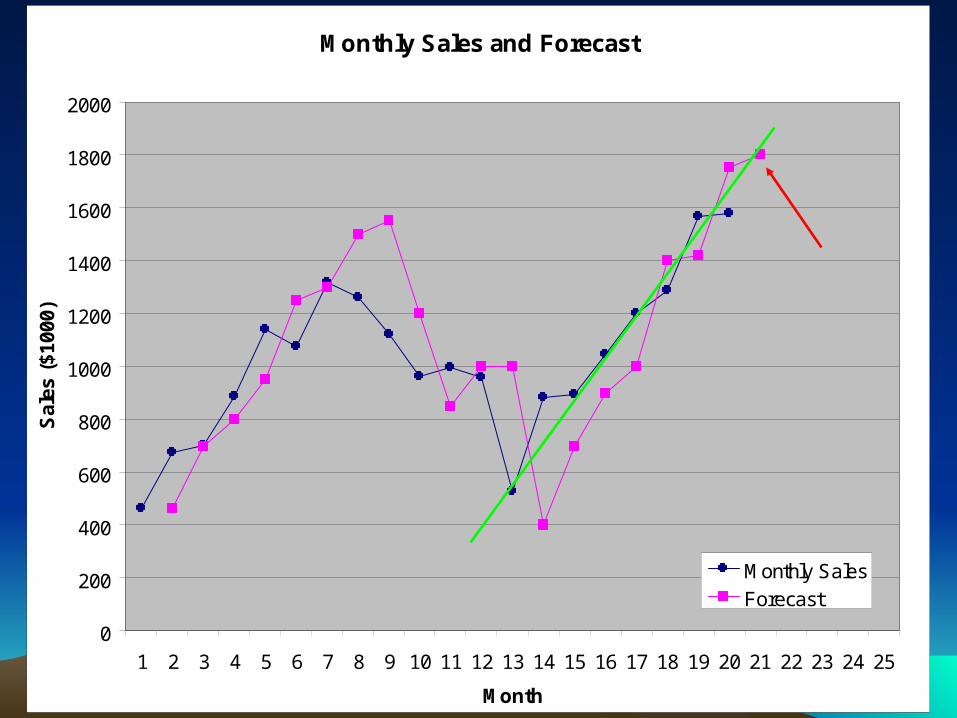
Heads will surely roll soon

Monthly Sales and Forecast
0
200
400
600
800
1000
1200
1400
1600
1800
2000
1 2 3 4 5 6 7 8 9 10 11 12 13 14 15 16 17 18 19 20 21 22 23 24 25
Month
Sal
es (
$100
0)
Monthly Sales
Forecast
Let’s be cautiously optimistic

Monthly Sales and Forecast
0
200
400
600
800
1000
1200
1400
1600
1800
2000
1 2 3 4 5 6 7 8 9 10 11 12 13 14 15 16 17 18 19 20 21 22 23 24 25
Month
Sal
es (
$100
0)
Monthly Sales
Forecast
Smithers calledbefore board

Monthly Sales and Forecast
0
200
400
600
800
1000
1200
1400
1600
1800
2000
1 2 3 4 5 6 7 8 9 10 11 12 13 14 15 16 17 18 19 20 21 22 23 24 25
Month
Sal
es (
$100
0)
Monthly Sales
Forecast

Monthly Sales and Forecast
0
200
400
600
800
1000
1200
1400
1600
1800
2000
1 2 3 4 5 6 7 8 9 10 11 12 13 14 15 16 17 18 19 20 21 22 23 24 25
Month
Sal
es (
$100
0)
Monthly Sales
Forecast
Perhaps we over reacted
Monthly Sales and Forecast
0
200
400
600
800
1000
1200
1400
1600
1800
2000
1 2 3 4 5 6 7 8 9 10 11 12 13 14 15 16 17 18 19 20 21 22 23 24 25
Month
Sal
es (
$100
0)
Monthly Sales
Forecast
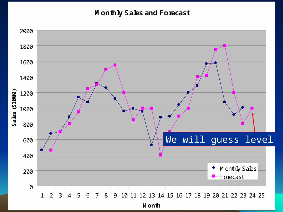
We will guess level

Monthly Sales and Forecast
0
200
400
600
800
1000
1200
1400
1600
1800
2000
1 2 3 4 5 6 7 8 9 10 11 12 13 14 15 16 17 18 19 20 21 22 23 24 25
Month
Sal
es (
$100
0)
Monthly Sales
Forecast
Back to normal!

Monthly Sales and Forecast
0
200
400
600
800
1000
1200
1400
1600
1800
2000
1 2 3 4 5 6 7 8 9 10 11 12 13 14 15 16 17 18 19 20 21 22 23 24 25
Month
Sal
es (
$100
0)
Monthly Sales
Forecast
Monthly Sales and Forecast
0
200
400
600
800
1000
1200
1400
1600
1800
2000
1 2 3 4 5 6 7 8 9 10 11 12 13 14 15 16 17 18 19 20 21 22 23 24 25
Month
Sal
es (
$100
0)
Monthly Sales
Forecast
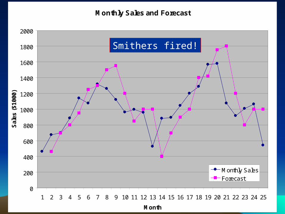
Smithers fired!

Part I: SEM & Introduction to Time Part I: SEM & Introduction to Time Series ModelsSeries Models
3. SEM for Mixed Designs with a PET study example

79
Structural Equation ModelingStructural Equation Modeling
Note: An endogenous (dependent, Y) variable (shown in blue) is one being pointed to (influences present in the model). An exogenous (independent, X) variable (shown in pink) is one with no arrows coming in (any existing influences are not present in the system under consideration). All variables are centered about their means.
Structural equation modeling can be used to estimate strength of relationshipbetween variables. Regression-style equations are generated from a path diagram, as shown below.
1 2
3 4 1
5 6 2
7 8 3
9 10 4
VS AMYG OFC
CG INS
THAL VS PUT
PUT VS CER
MFC INS THAL
80
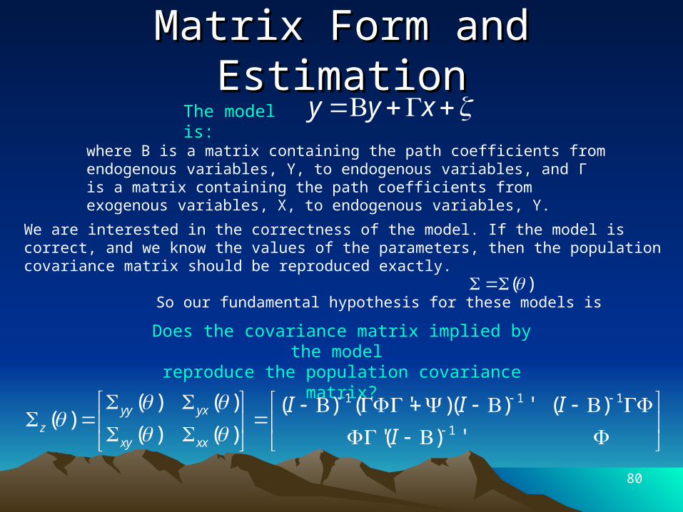
We are interested in the correctness of the model. If the model is correct, and we know the values of the parameters, then the population covariance matrix should be reproduced exactly.
So our fundamental hypothesis for these models is
Matrix Form and EstimationMatrix Form and EstimationThe model is: y y x
where Β is a matrix containing the path coefficients from endogenous variables, Y, to endogenous variables, and Γ is a matrix containing the path coefficients from exogenous variables, X, to endogenous variables, Y.
( )
Does the covariance matrix implied by the model reproduce the population covariance matrix?
1 1 1
1
( ) ( ) ( ) ( ' )( ) ' ( )( )
( ) ( ) '( ) 'yy yx
zxy xx
I I I
I

81
Maximum Likelihood EstimationMaximum Likelihood Estimation
1log ( ) ( ) log ( )MLF tr S S p q
122 11
2( ; ) (2 ) exp 'p q
f z z z
When observations of each variable are taken from N subjects, the likelihood function is:
( )22 11
21
( ) (2 ) ( ) exp ' ( )N p q N N
i
L z z
Indeed we estimate the parameters through the maximum likelihood method, assuming the measured variables are distributed multivariate normal. The joint distribution function is shown below.
We can calculate a standard error for each parameter to use in analysis of significance (each parameter has an asymptotic normal distribution. The standard errors come from the asymptotic covariance matrix:
1
22ˆ1 '
MLFACOV E
N
The traditional fit function is a manipulation of the likelihood function. We minimize the following function over all model parameters to choose their values.
82
Example Results for Brain Functional Example Results for Brain Functional Pathway ExamplePathway Example
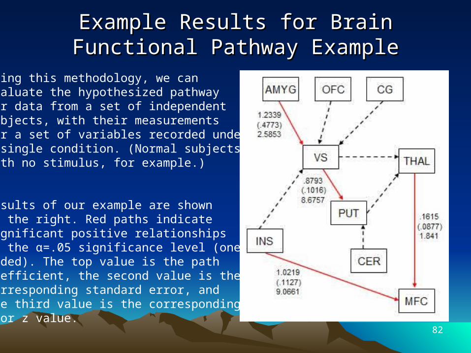
Using this methodology, we can evaluate the hypothesized pathway for data from a set of independent subjects, with their measurements for a set of variables recorded under a single condition. (Normal subjects with no stimulus, for example.)
Results of our example are shownat the right. Red paths indicate significant positive relationshipsat the α=.05 significance level (one-sided). The top value is the path coefficient, the second value is the corresponding standard error, and the third value is the corresponding t or z value.

83
SEM Software CapabilitySEM Software CapabilitySAS
PROC CALIS implements estimation of single-group SEMs. As of version 9.1.3, SAS has no multiple group comparison capability. In version 9.2, SAS has incorporated a new procedure called TCALIS that is capable of the multiple group comparisons other software does. (SAS technical support)
LISREL Implements estimation of single-group SEMs. LISREL does have multiple group comparison capability by restraining parameters equal in the
goodness-of-fit comparison framework. LISREL uses less intuitive key words and its code-generating user interface is not always accurate. (Joreskog 1996)
EQSImplements estimation of single-group SEMs. EQS also has multiple group comparison capability by restraining parameters equal in the goodness-of-fit comparison framework. The user interface is easy to use and understand and generates code accurately. EQS is also capable of estimating multilevel SEMs.(Byrne 2006)
These programs are good if your model fits your data well, but they are onlyappropriate for independent group analyses. We need a new method for correlated data.

84
Example of Mixed Design Data:
The Brain Reward Study
The study measures two groups of subjects, 16 normal subjects and 25 cocaine abusers, each under two conditions. Subjects are told they will receive either placebo or methyl-phenidate (a cocaine-like substance) and they receive placebo before the PET scan is taken. As a result, there are two factors of interest—group membership and drug expected.
The reward pathway is of interest. We are interested in whether group membership and expectation affect the strength of each path.
The regions of interest are: the amygdala (AMYG), orbital frontal cortex (OFC), anterior cingulate gyrus (CG), ventral striatum (VS2), thalamus (THAL), insula (INS), putamen (PUT), and motor frontal cortex (MFC).
NormalGroup 0
AbusersGroup 1
No Drug Drug No Drug Drug

85
Existing Methods for Multiple Group or Existing Methods for Multiple Group or Repeated Measures AnalysisRepeated Measures Analysis
To date, multiple groups and repeated measures are not handled at the same time. This is illustrated in the title of chapter four of John C. Loehlin’s text, Latent Variable Models, “Fitting Models Involving Repeated Measures or Multiple Groups.” This text, published in 2004, reports that models can have either structure, but not both.
Currently, there is only one method available for comparison of independentgroups in the context of SEM. This Nested Goodness-of-Fit method is implemented in the current SEM software as the only option for multiple-groupcomparison (Jaccard and Wan 1996).
The current SEM model for repeated measures data is known as LatentGrowth Modeling (Meredith and Tisak 1990).
Our data consists of measurements from two groups, each evaluated under twoconditions, so we will need an analysis method that can manage both.

86
SEM for Mixed Designs: SEM for Mixed Designs: Multiple Groups with Repeated MeasuresMultiple Groups with Repeated Measures
For each path in the hypothesized diagram, we reparametrize the path coefficientto reflect possible changes from the normal subject receiving placebo due to group membership and receiving methylphenidate.
Dataset 1: Normal subjects receiving placebo (group=0, drug=0)Dataset 2: Normal subjects receiving methylphenidate (group=0, drug=1)Dataset 3: Cocaine abusers receiving placebo (group=1, drug=0)Dataset 4: Cocaine abusers receiving methylphenidate (group=1, drug=1)

87
Because we have reparametrized path coefficients with multipliers of 0 and 1, for each group and condition combination, we will have a model that contains summed path coefficients preceding each variable. Therefore, the variables in the model are still distributed as multivariate normal.
SEM for Mixed Designs: Brain Reward StudySEM for Mixed Designs: Brain Reward Study
1 2 3 4 1
5 6 2
7 8 4
9 10 5
vs amyg ofc cg ins
thal vs put
put vs cer
mfc ins thal
ò
ò
ò
ò
1 2 4 5 7 8 10 11 1
13 14 16 17 2
19 20 22 23 3
25 26 28 29 4
vs amyg ofc cg ins
thal vs put
put vs cer
mfc ins thal
ò
ò
ò
ò
Original model:
Mixed Model (2 Groups under 2 Conditions):
Mixed Model, considering group 1 under drug 0:
1 2 3 4 5 6
7 8 9 10 11 12 1
13 14 15 16 17 18 2
19 20 21 22 23 24
* * * *
* * * *
* * * *
* * * *
vs amyg g amyg d amyg ofc g ofc d ofc
cg g cg d cg ins g ins d ins
thal vs g vs d vs put g put d put
put vs g vs d vs cer g cer d cer
ò
ò
3
25 26 27 28 29 30 4* * * *mfc ins g ins d ins thal g thal d thal
ò
ò

88
Implementation of SEM for Mixed DesignsImplementation of SEM for Mixed Designs
1 1 10 0 0 0 0 0 0 0 0
0 10 0 0 0
( ) ( ' )( ) ( )( )
'( )
I I I
I
We can construct the Β and Γ matrices as shown below. (Below we consider only group 0, as group 1’s matrices can be constructed similarly.)
00 000 0
01 01
0 0,
0 0
Once we have Φ and Ψ, shown on the next slide, we can construct the implied model covariance matrix as in the single-group case, shown below.
y y x
89
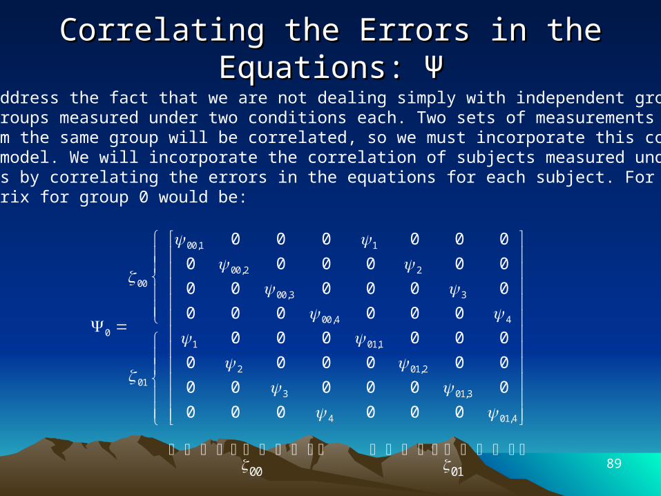
Correlating the Errors in the Equations: Correlating the Errors in the Equations: ΨΨ
We must address the fact that we are not dealing simply with independent groups, but two groups measured under two conditions each. Two sets of measurementstaken from the same group will be correlated, so we must incorporate this correlationinto the model. We will incorporate the correlation of subjects measured under twoconditions by correlating the errors in the equations for each subject. For example, the Ψ matrix for group 0 would be:
00,1 1
00,2 200
00,3 3
00,4 40
1 01,1
2 01,2
013 01,3
4 01,4
00 01
0 0 0 0 0 0
0 0 0 0 0 0
0 0 0 0 0 0
0 0 0 0 0 0
0 0 0 0 0 0
0 0 0 0 0 0
0 0 0 0 0 0
0 0 0 0 0 0

90
Correlating the Errors of the Correlating the Errors of the Independent Variables: Independent Variables: ΦΦ
Additionally, to incorporate the correlation of the repeated measures, we will correlate the errors of the independent variables, X through the Φ matrix.
To incorporate correlation of errors in the independent variables, we add terms to the Φ matrix that correlate vectors the errors for the repeated measures, as shown below. X1 contains measures of group 0 under both conditions. The two conditions’ errors should be correlated, as should those for group 1. We allow all errors to be correlated freely.
00 00 12
01 12 01
00 01
'
X X
X
X
1 2 3 4 5
6 7 8 9 10
12 11 12 13 14 15
16 17 18 19 20
21 22 23 24 25

91
Estimation of SEM for Mixed DesignsEstimation of SEM for Mixed DesignsWe can consider the likelihood function to be a product of the likelihood functions of the two independent groups. Each group will have 18 variables (9 for each condition) that are distributed as multivariate normal. Note: All variables have been centered about their means.
Consider the 18 variables that comprise measurements from group 0. Their joint distribution is
122 11
0 0 0 0 0 02( ; ) (2 ) exp ' .p q
f z z z
0( ) 0022
0
110 0,1 0,2 0, 0 0, 0 0,2
1
( ) ( ; ( )) ( ; ( )) ( ; ( )) (2 ) ( ) exp ' ( )NN p q
N
N i ii
L f z f z f z z z
0 1( ) ( )0 10 12 22 21 11 1
0 0 1 12 21 1
( ) (2 ) ( ) exp ' ( ) (2 ) ( ) exp ' ( )N NN p q N p q
N N
i i i ii i
L z z z z
We take N observations of Z, from N different subjects from our chosen group, and the resulting likelihood function for Z is
The likelihood function for group 1 can be constructed in the same way. Then to create the full likelihood function, we can multiply the independent group likelihoods.
92
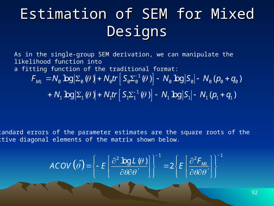
Estimation of SEM for Mixed DesignsEstimation of SEM for Mixed Designs
10 0 0 0 0 0 0 0 0 0
11 1 1 1 1 1 1 1 1 1
log ( ) ( ) log ( )
log ( ) ( ) log ( )
MLF N N tr S N S N p q
N N tr S N S N p q
As in the single-group SEM derivation, we can manipulate the likelihood function intoa fitting function of the traditional format:
The standard errors of the parameter estimates are the square roots of therespective diagonal elements of the matrix shown below.
11
22 log ( )ˆ 2 MLFLACOV E E

93
Numerical Implementation of Numerical Implementation of SEM for Mixed DesignsSEM for Mixed Designs
1. A MATLAB script file creates the list of parameters to be estimated and setsstarting values (as suggested by Bollen).
2. The script calls built-in MATLAB function fminunc to minimize the likelihood-based fitting function derived on the previous slide, yielding the parameter estimates.
3. We calculate standard errors by generating the Hessian matrix of secondderivatives of the fitting function numerically, evaluated at the parameter estimates.
4. Estimates and standard errors are recorded and used to generate 95% and 90% confidence intervals about the parameter estimates. These are used todetermine whether the null hypothesis should be rejected. If so,the corresponding path (or group / expectation effect on the path) is significant.
0 : 0iH

94
Analysis of the Brain Reward StudyAnalysis of the Brain Reward Study
Our model:
Our data:
Our goal:
1 2 3 4 5 6
7 8 9 10 11 12 1
13 14 15 16 17 18 2
19 20 21 22 23 24
* * * *
* * * *
* * * *
* * * *
vs amyg g amyg d amyg ofc g ofc d ofc
cg g cg d cg ins g ins d ins
thal vs g vs d vs put g put d put
put vs g vs d vs cer g cer d cer
ò
ò
3
25 26 27 28 29 30 4* * * *mfc ins g ins d ins thal g thal d thal
ò
ò
Our data consists of measurements from two groups, measured under each of two conditions. Group 0 consists of normal subjects and group 1 consists of cocaine abusers. Each is subjected to receiving placebo (drug=0) and the cocaine-like substance methylphenidate (drug=1). All subjects underconsideration have expected to receive placebo.
The goal of this study is to determine whether group membership and drug affect the strength of connectivity (path coefficients) in the reward network.
95
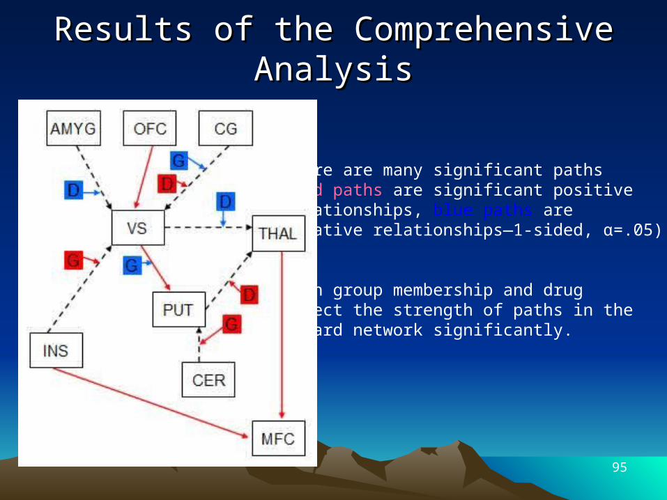
Results of the Comprehensive AnalysisResults of the Comprehensive Analysis
There are many significant paths (red paths are significant positive relationships, blue paths are negative relationships—1-sided, α=.05).
Both group membership and drug affect the strength of paths in the reward network significantly.

Part II: PCNA and Bootstrap Part II: PCNA and Bootstrap ResamplingResampling
1. Partial Correlation Network Analysis

97
PCNAPCNA: Generating a Path Diagram: Generating a Path DiagramWhen there is not a hypothesized diagram for a SEM analysis, we can generatea path diagram using partial correlation network analysis.
In 2006, Marrelec discussed the concept of detecting an underlying connectivity network in data, and the methods for analysis. He noted the importance of detection without hypothesized relationships, as SEM requires. In 2007, Marrelec et. al. published a work praising the use of Partial Correlation Network Analysis (PCNA) in conjunction with SEM.
Partial correlation analysis is a technique that allows us to investigate the relationship between two variables free of influence from other variables.
Consider two variables, X and Y. We want to know the correlation of X and Y while controlling for Z. The most intuitive way to understand partial correlation is to consider two regressions.
1 1 1
2 2 2
X a b Z
Y a b Z
ò
ò
1 1 2 2ˆ ˆˆ ˆ( , ) ( , | )Corr X a b Z Y a b Z PartialCorr X Y Z
98
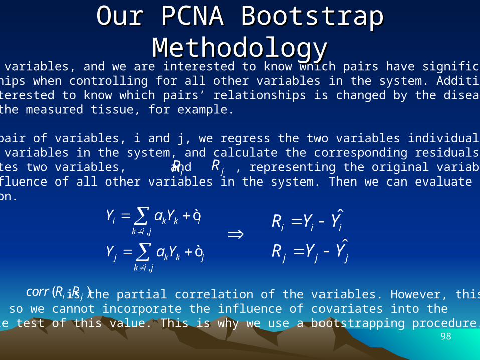
We have N variables, and we are interested to know which pairs have significantrelationships when controlling for all other variables in the system. Additionally,we are interested to know which pairs’ relationships is changed by the diseasestate of the measured tissue, for example.
For each pair of variables, i and j, we regress the two variables individually on all other variables in the system, and calculate the corresponding residuals. This creates two variables, and , representing the original variables free of the influence of all other variables in the system. Then we can evaluate their correlation.
Our PCNA Bootstrap MethodologyOur PCNA Bootstrap Methodology
jR
ˆ
ˆi i i
j j j
R Y Y
R Y Y
iR
,
,
i k k ik i j
j k k jk i j
Y a Y
Y a Y
ò
ò
( , )i jcorr R R is the partial correlation of the variables. However, this is justone number, so we cannot incorporate the influence of covariates into the significance test of this value. This is why we use a bootstrapping procedure.
Part II: PCNA and Bootstrap Part II: PCNA and Bootstrap ResamplingResampling
2. Bootstrap Resampling

100
Bootstrap ResamplingBootstrap Resampling
Use each resample to calculate the partial correlation. Now we have a population of n measurements for each pair of variables. If we perform this analysis on our two datasets individually, we will have 1000 estimates of partial correlation for the normal tissue and 1000 estimates for the diseased tissue.
We have our original sample of m subjects. 1 2 3 m…
Select one of them at random, and then replace it before randomly selecting the next.Repeat this m times.
Now we have a sample of m subjects consisting of subjects from the original sample. However, some subjects may be repeated, and some subjects from the original sample may not be present in our resample.
The idea behind bootstrapping is resampling with replacement.
1
i
2 3 m…

101
Bootstrap ResamplingBootstrap ResamplingWe will let the significance of the relationships in the normal dataset represent the general significance of partial correlation among variables in the system.
We can create a difference variable to estimate the difference of the partial correlationbetween the normal tissue and diseased tissue. The significance of the differences represents the influence of disease on the partial correlation between variables.
The results we must evaluate are two lists of partial correlations (those for the normal tissue, and those for the diseased tissue).
Normal Diseased Difference
V1 W1 V1 – W1
V2 W2 V2 – W2
V3 W3 V3 – W3
… … …
Sort the normal and difference variables. If 0 is contained in the middle 95% of the observations, then we would say the relationship or influence of disease is insignificant for this pair of variables. (This is called the percentile method).
102
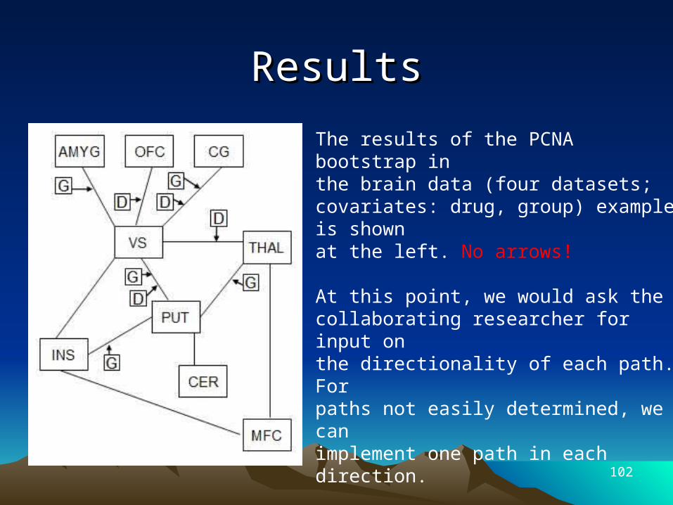
ResultsResults
The results of the PCNA bootstrap in the brain data (four datasets; covariates: drug, group) example is shown at the left. No arrows!
At this point, we would ask the collaborating researcher for input onthe directionality of each path. For paths not easily determined, we canimplement one path in each direction.
The results would be a hypothesizedrelationship that can be verified usingstructural equation modeling with an independent data set.

103
Current WorkCurrent Work
SEM with both continuous and categorical variables (shown next.)

Microbiomemeasured by dCT
PhenotypeCD / UC / non IBD
GenotypeSNPs
Multiple Regression
Logistic Regression
Multiple Regression
NOD2 ATG16L1
IRGM IL12B NKX2_3 MST1
Logistic
Regression
Logistic Regression
Multiple Regression (indeed GLM)
Pathway Assumptions and Statistical Models
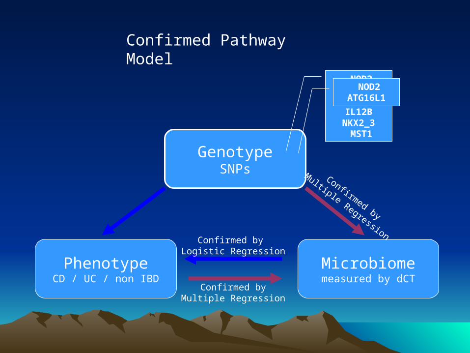
Microbiomemeasured by dCT
PhenotypeCD / UC / non IBD
GenotypeSNPs
Confirmed by
Multiple RegressionConfirmed by
Logistic Regression
Confirmed byMultiple Regression
NOD2 ATG16L1
IRGM IL12B NKX2_3 MST1
Confirmed Pathway Model
NOD2 ATG16L1
[1] Bollen, K.A., Structural Equations with Latent Variables. 1989: John Wiley and Sons, Inc.[2] Blalock, H.M., Causal Inferences in Nonexperimental Research. 1964: University of North Carolina Press.[3] Duncan, O.D., Path analysis: Sociological examples. American Journal of Sociology, 1966. 72: p. 1-16.[4] Wolfle, L.M., The Introduction of Path Analysis to the Social Sciences, and Some Emergent Themes: An Annotated Bibliography. Structural Equation Modeling, 2003. 10(1): p. 1-34.[5] Joreskog, K. and D. Sorbom, LISREL 8: User's Reference Guide. 1996: Scientific Software International, Inc.[6] Jaccard, J. and C.K. Wan, LISREL Approaches to Interaction Effects in Multiple Regression. Quantitative Applications in the Social Sciences. 1996: Sage Publications.[7] Byrne, B.M., Structural Equation Modeling with EQS: Basic Concepts, Applications, and Programming . Second ed. 2006: Lawrence Erlbaum Associates.[8] Coenders, G., J.M. Batista-Foguet, and W.E. Saris, Simple, Efficient and Distribution-free Approach to Interaction Effects in Complex Structural Equation Models. Quality & Quantity, 2008. 42(3): p. 369-396.[9] Cronbach, L.J. and N. Webb, Between class and within class effects in a reported aptitude x treatment interaction: a reanalysis of a study by G. L. Anderson. Journal of Educational Psychology, 1979. 67: p. 717-724.[10] Muthen, B., Means and covariance structure analysis of hierarchical data. UCLA Statistics series. Vol. #62. 1990.[11] Marcoulides and Schumacker, eds. Advanced Structural Equation Modeling. 1996.[12] Scientific Software International. Multilevel structural equation modeling. 2005-2008 [cited 2008; LISREL implementation of multilevel SEM]. Available from: http://www.ssicentral.com/lisrel/techdocs/Session12.pdf.[13] Garson GD. Statnotes: Partial Least Squares. 1998, 2008, 2009 [cited 2009; Introduction to Partial Least Squares SEM and Regression]. Available from: http://faculty.chass.ncsu.edu/garson/PA765/pls.htm.[14] Hoyle RH. Statistical Strategies for Small Sample Research. 1999: Sage Publications.[15] Joreskog KG and Wold H, The ML and PLS Techniques for Modeling with Latent Variables, in Systems under indirect observation: causality, structure, prediction, K.G. Joreskog and H. Wold, Editors. 1982.[16] Tenenhaus M, Vinzi VE, Chatelin Y-M, Lauro C. PLS path modeling. Computational Statistics & Data Analysis, 2005. 48: p. 159-205.[17] Wold H, ed. The Fix-Point Approach to Interdependent Systems. 1981, North-Holland Publishing Company.[18] Wold H. Estimation of Principal Components and Related Models by Iterative Least Squares. Multivariate analysis; proceedings of an international symposium held in Dayton, Ohio, June 14-19, 1965, 1966: p. 391-420.[19] Wold H, PLS for multivariate linear modeling, in QSAR: Chemometric methods in molecular design: Methods and principles in medicinal chemistry, H.v.d. Waterbeemd, Editor. 1994.[20] Wold H, Partial Least Squares, in Encyclopedia of Statistical Sciences. 2006, John Wiley & Sons, Inc.
Selected ReferencesSelected References

[21] Volkow, N.D., et al., Expectation Enhances the Regional Brain Metabolic and the Reinforcing Effects of Stimulants in Cocaine Abusers. The Journal of Neuroscience, 2003. 23(36): p. 11461-11468.[22] Crowder, M.J. and D.J. Hand, Analysis of Repeated Measures. 1990: Chapman & Hall.[23] Cudeck, R., S. du Toit, and D. Sorbom, eds. Structural Equation Modeling: Present and Future, A Festschrift in honor of Karl Joreskog. 2001, Scientific Software International.[24] Blackwell, E., C.F.M.D. Leon, and G.E. Miller, Applying Mixed Regression Models to the Analysis of Repeated-Measures Data in Psychosomatic Medicine. Psychosomatic Medicine, 2006. 68: p. 870-878.[25] Garson, G.D. Statnotes: Topics in Multivariate Analysis, Structural Equation Modeling. 1998, 2008 [cited 2008; Introduction to SEM]. Available from: http://faculty.chass.ncsu.edu/garson/PA765/partialr.htm.[26] Krzanowski, W.J. and F.H.C. Marriott, Multivariate Analysis Part 2: Classification, covariance structures and repeated measurements. 1995, New York: Halsted Press.[27] Rovine, M.J. and P.C.M. Molenaar, A LISREL Model for the Analysis of Repeated Measures With a Patterned Covariance Matrix. Structural Equation Modeling, 1998. 5(4): p. 318-343.[28] Vittinghoff, E., et al., Regression Methods in Biostatistics: Linear, Logistic, Survival, and Repeated Measures Models . 2005: Springer.[29] Diggle, P.J., et al., Analysis of Longitudinal Data. Second ed. Oxford Statistical Science Series. 2002.[30] Monahan, J.F., Numerical Methods of Statistics. 2001: Cambridge University Press.[31] Gill, P.E., W. Murray, and M.H. Wright, Practical Optimization. 1981, London: Academic Press, Inc.[32] Stanghellini, E. and N. Wermuth, On the identification of path analysis models with one hidden variable. Biometrika, 2005. 92(2): p. 337-350.[33] Dunn, G., B. Everitt, and A. Pickles, Modelling Covariances and Latent Variables Using EQS. 1993: Chapman & Hall.[34] Skrondal, A. and S. Rabe-Hesketh, Generalized Latent Variable Modeling: Multilevel, Longitudinal, and Structural Equation Models. 2004: Chapman & Hall/CRC.[35] Marrelec, G., et al., Using partial correlation to enhance structural equation modeling of functional MRI data. Magnetic Resonance Imaging, 2007. 25: p. 1181-1189.[36] Garson, G.D. Statnotes: Partial Correlation. 1996, 2008 [cited 2008; Introduction to Partial Correlation]. Available from: http://faculty.chass.ncsu.edu/garson/PA765/partialr.htm.[37] Rees, D.G., Foundations of Statistics. 1987: CRC Press.[38] Lunneborg, C.E. and J.P. Tousignant, Efron's Bootstrap with Application to the Repeated Measures Design. Multivariate Behavioral Research, 1985. 20: p. 161-178.[39] Berkovits, I., G.R. Hancock, and J. Nevitt, Bootstrap Resampling Approaches for Repeated Measure Designs: Relative Robustness to Sphericity and Normality Violations. Educational and Psychological Measurement, 2000. 60: p. 877-892.[40] Seco, G.V., et al., A Comparison of the Bootstrap-F, Improved General Approximation, and Brown-Forsythe Multivariate Approaches in a Mixed Repeated Measures Design. Educational and Psychological Measurement, 2006. 66(35-62).[41] Fisher, R.A., The distribution of the partial correlation coefficient. Metron, 1924. 3-4: p. 329-332.[42] Marrelec, G., P. Bellec, and H. Benali, Exploring Large-Scale Brain Networks in Functional MRI. 2006.