Annual Miles Drive Used Car Prices

Maxim EngersUniversity of Virginia

Monica HartmannUniversity of St. Thomas

Steven Stern�

University of Virginia

January 2008

Abstract

Abstract: This paper investigates whether changes in vehicle�s netbene�ts, proxied by annual miles driven, explain the observed patternof price declines over a vehicle�s life. We �rst model the household�sdecision on how much to drive each of its vehicles using two approaches.The �rst is a basic nonstructural approach that restricts the relationshipbetween annual mileage and the household�s characteristics to be linearover the vehicle�s life. The second is a structural model that allows fornonlinearity. It takes into account how the composition of vehicles owned- the number and the age distribution of the vehicles - in�uence whichhousehold car is drive on a particular trip and how much it is driven. Wethen use the mileage estimates to determine if the variation in household-mileage decision across brands can explain the pricing paths observed forused cars. Results indicate that the structural estimates of the householdmileage decision better predict changes in prices over a vehicle�s life. Thesuperiority of the structural estimates implies that the e¤ect vehicle agehas on mileage decisions (and consequently the vehicle�s market value)cannot be estimated independently of household characteristics and thecomposition of the vehicle stock owned. Thus, one must account for thesefeedback e¤ects when using mileage to control for exogenously depreciatedquality. The results strongly suggest that variation in net bene�ts ofspeci�c brand/vintage vehicles signi�cantly a¤ects variation in used carprices.

Keywords: Annual Miles, Used Car Prices, Durable Goods

�Corresponding Author: Steven Stern, Department of Economics, University of Virginia,Charlottesville, Va 22904; sns5r@virginia.edu; (434)924-6754; fax: (434)982-2904.

1

1 Introduction

The net �ow of bene�ts provided by a vehicle can be viewed as the value oftransportation services provided minus the maintenance and repair costs in-curred. Suppose that the annual mileage serves as a proxy for this �ow. Thenannual miles may explain the observed drop in used car prices over a vehicle�sworking life. This paper investigates what factors in�uence household miles de-cisions and whether these choices are consistent with the observed pricing pathsof these assets.There are a number of alternative explanations for why used car prices

decline with age, the pricing path we observe. One explanation is obsolescencedue to styling changes or quality improvements, such as airbags, advancementsthat are available in newer cars.. For example, Purohit (1992) �nds that therate of depreciation on small vehicles increases with the introduction of a newermodel with greater horsepower. However, this obsolescence e¤ect, although sig-ni�cant, is small relative to other durable goods that have more radical modelchanges. Thus, it seems unlikely that improvements in car quality or in stylingchanges can explain the magnitude of price declines and the variation in pricedeclines over brands. Another explanation is that the adverse selection problemincreases as vehicles age.1 For instance, Engers et al. (2005) provide evidencethat the used car market for four year old vehicles su¤ers more from adverseselection than the one year old market. Still, it is questionable whether this issu¢ ciently large to drive the decline in prices.To determine if variation in vehicle usage (i.e., annual miles) helps explain

the observed price declines for automobiles, we �rst model the household vehicleannual miles decision and then establish the empirical relationship between an-nual miles and used car prices. To estimate the household-vehicle annual milesdecision, we estimate two models: a basic OLS model and a structural model.The OLS model assumes a linear relationship between household characteristicsand annual miles. In contrast, the structural model allows for nonlinear in�u-ence of changes in car portfolios and household demographic characteristics onhow a vehicle�s age a¤ects annual miles. For instance, it takes into accounthow the portfolio of vehicles owned - the number and the age distribution of thevehicles - in�uences a household�s decision to drive a car on a particular tripand how much it is driven. Our results indicate that the structural estimatesof the household mileage decision better explain the observed pattern of pricedecline over a vehicle�s life than the OLS model. Furthermore, the structuralmodel also allows us to decompose the age e¤ect of mileage on prices into threeparts: a direct aging e¤ect, a household-car portfolio e¤ect, and a householddemographics e¤ect. The �rst component captures the direct e¤ect vehicle age

1One may argue that because of the vast improvements in car quality that adverse selectionis no longer a serious problem. According to J.D. Power & Associates�Survey of Initial CarQuality, the average number of car problems per 100 vehicles has declined signi�cantly in thelast 7 years. Despite these improvements, there is still variation across brands (e.g., Lexus- 81, Mazda - 149, Suzuki -151). Furthermore, these �gures provide no indication aboutthe variability within a brand to make a statement that the adverse selection problem hasweakened.

2

has on annual miles. The portfolio e¤ect re�ects the fact that annual milesdepend on the characteristics of the stock of vehicles the household owns. Forexample, households often choose to drive the newer, more dependable vehicleon long trips. Finally, the third e¤ect measures the in�uence household charac-teristics, such as the number of drivers and whether or not the household livesin an urban area, has on driving patterns. The superiority of the structuralmodel suggests that one cannot estimate the e¤ect age has on annual milesdecisions independent of household characteristics and household-car portfoliochoices. Thus, studies that measure the impact of adverse selection on prices,for instance, miss these feedback e¤ects if they use only annual miles to controlfor exogenously depreciated quality. They also must control for di¤erence indriving patterns across households, vehicle age, and brand.Our model of vehicle utilization and used car prices di¤ers from previous

studies. Goldberg (1998), using micro-level data, models annual miles as afunction of household demographic and vehicle characteristics as well as char-acteristics of the household�s stock of vehicles (e.g., number of vehicles, averageage of the stock, age of the youngest vehicle). Our study of vehicle utilizationdi¤ers in three ways. First, we examine driving patterns over a vehicle�s en-tire working life and not just in its �rst year. Second, we investigate whetherdriving patterns are constant across brands. Quality deterioration is known tovary across brands. Thus, the value of the transportation services may vary bybrand and lead to di¤erent patterns of car usage over the vehicle�s working life.Third, we examine if the amount a given vehicle is driven depends on its qualityrelative to all of the other vehicles owned by the household and not just theaverage quality of the household�s vehicle stock.Our model of the process that generates used car prices di¤ers from Alberini

et al. (1995) (AHM1) and Alberini et al. (1998) (AHM2) as well. They esti-mate the distribution of vehicle values based on what owners would accept toscrap their vehicles.2 Because their sample includes only vehicles that qualifyfor a vehicle scrappage program, the average age is 17 years with a minimumand maximum age of 13:5 and 32 years, respectively. Thus, they estimate thedistribution of vehicle values for only the right tail of the age distribution. Inaddition to expanding the range of ages analyzed, our model allows annual milesto play a di¤erent role in determining vehicle values. AHM1 and AHM2 modelhousehold and vehicle characteristics directly determining the vehicle�s value.Instead, we model these characteristics a¤ecting the vehicle�s value only indi-rectly through annual miles. Unlike AHM1 and AHM2, we �nd that householdcharacteristics are determinants of a vehicle�s value, but through their in�uenceon annual miles. The intuition behind our result is that vehicle and householdcharacteristics a¤ects a household�s driving patterns and consequently a¤ectsthe vehicle�s value as well.Our �nding that vehicle age a¤ects annual miles nonlinearly also has implica-

tions for other automobile-related studies. For example, both Goldberg (1998)2The amount a household is willing to accept to scrap its car is weakly tied to the car�s

net bene�ts of transportation services. Alternatively, we use Kelly Blue Book used car pricesto proxy the car�s value that captures both supply and demand market conditions.

3

and Verboven (2002) assume annual miles are constant over the vehicle�s life.Goldberg (1998) uses a model of vehicle utilization demand to estimate elastic-ity of annual miles demand with respect to gasoline cost per mile. Substitutionpatterns derived from this model take into account di¤erences in fuel e¢ ciencyacross new and used vehicles. Because it does not allow for di¤erences in ve-hicle usage across age, the model overestimates annual miles demand for oldervehicles and the reverse for newer ones, potentially biasing elasticity estimates.Several data sources are used to establish the relationship between annual

miles and used car prices. Data from the National Personal TransportationSurvey allows us to track how much households drive each vehicle they own. Thesurvey also provides information on demographic characteristics that in�uencethe amount of driving. Detailed pricing information is collected from Kelly BlueBooks. Finally, observed scrappage rates by brand are used to estimate jointlythe parameters of the process that determines used car prices and scrappagerates, correcting for a potential selection bias problem in the price estimates.The layout of the paper is as follows: Section 2 considers a simple dynamic

model of the relationship between annual miles and price to motivate the re-mainder of the paper. Section 3 describes the annual miles data and thenpresents two alternative models to estimate household annual miles decisions.Section 4 presents the model that jointly estimates prices and scrappage rates tocontrol for a selection bias. Section 5 examines the relationship between annualmiles and price and demonstrates that the structural model of household annualmiles decisions best explains the price decline observed in the used car market,and Section 6 concludes.

2 Dynamic Model of Annual Miles and Price

The empirical results of this paper show that variation across brands in ratesof decline in annual miles explains variation in price declines across brands. Inorder to understand these results, consider the following simple model of annualmiles and prices. Suppose that the bene�t �ow net of costs derived from owninga car of brand b and age t is denoted by fbt which monotonically decreases witht. We think of annual miles, the �ow of miles driven in one year, as a proxyfor fbt. Throughout the paper, we are interested in the �ow of miles drivenin one year rather than in the stock of miles previously driven. For simplicity,suppose that the rate of decline in fbt is uniform over time (but can vary frombrand to brand), so that

fbt = &fb + �fb t (1)

where &fb > 0 and �fb < 0.

If � is the per-period discount factor, the value Wbt to any consumer of acar of brand b of age t satis�es a simple recursion condition: the car can eitherbe sold at price pbt or kept for the period, generating current net surplus of fbt.Thus

Wbt = maxffbt + �Wbt+1; pbtg (2)

4

Competition among buyers and the possibility of free disposal ensure that

pbt = maxfWbt; 0g: (3)

Because fb0 > 0 and fbt decreases at a constant rate, there is a (unique)�nal period t�b in which the vehicle provides a positive service �ow;

9t�b : pbt�b =Wbt�b> 0; pbt�b+k =Wbt�b+k

= 0 8k > 0: (4)

Let �Wbs denote the change inWbs when s is increased by one, so that�Wbs =Wbs+1 �Wbs. In all periods t � t�b , Wbt = fbt + �Wbt+1, and so

�Wbt = �fb + ��Wbt+1 8t < t�b : (5)

By induction on t�b � t, it follows that

�Wbt < 0 8t < t�b ; (6)

so prices decline monotonically until the car becomes worthless. Di¤erentiatinggives

@�Wbt+1

@�fb= 1 + �

@�Wbt+1

@�fb8t < t�b ; (7)

and, again by induction on t�b � t,

@�Wbt+1

@�fb> 0 8t < t�b : (8)

This last relationship says that, if we compare two di¤erent brands, thenthe one whose annual miles decline at a faster rate (i.e. whose �fb is a largernegative number) will also be the one whose price declines faster. The goal ofthis paper is to see whether this relationship between the annual miles changesand price changes is found in the data we examine.

3 Annual Miles

This section presents factors that in�uence driving patterns. We �rst examinerelationships in the raw data between annual miles and household and vehi-cle characteristics. Then a simple OLS regression of log annual miles on thesecharacteristics provides insight into the in�uence of each factor on driving pat-terns. Finally, we present a structural model that links annual miles choices withhousehold characteristics and the quality of the vehicles the household owns.

5

3.1 Data

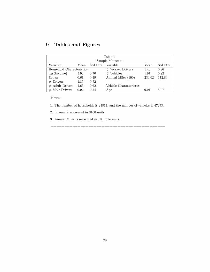
The annual miles data for this study come from the Nationwide Personal Trans-portation Survey, 1995 (NPTS). The NPTS is a sample of 47293 vehicles ownedby 24814 households. We observe some characteristics of each household inthe sample such as family income, location characteristics (e.g., urban), and thenumber of drivers disaggregated by age, gender, and work status. Also, weobserve each vehicle owned by the household, its age, brand, and annual milesdriven.Table 1 reports moments of the data. The average household has a log

income of 5:93 ($37600)3 with 1:85 drivers and 1:91 vehicles. It has 0:2 teenagedrivers and 0:45 drivers who do not work, and it drives 23462 miles per year.The average vehicle in the sample is 9:91 years old.Figure 1 presents broad brand categories which will be disaggregated further

for most of the analysis. The categories included in the analysis are GM (Buick,Chevrolet, Geo, Oldsmobile, Pontiac, Saturn); Japanese (Honda, Mazda, Mit-subishi, Nissan, Subaru, Toyota); Ford (Ford, Mercury); Luxury (AmericanLuxury,4 European Luxury,5 Japanese Luxury6); Chrysler (Chrysler, Dodge,Plymouth); European (Volkswagen, Volvo); Truck;7 and Other.8 Trucks arethe most common category. Our method of aggregation is somewhat di¤er-ent than others in the literature. Goldberg (1998) aggregates into categoriesof �subcompact,� �compact,� �intermediate,� �standard,� �luxury,� �sports,��pick-up truck,�and �van.� We feel our aggregation scheme is better for ourpurposes because we think there are more likely to be brand e¤ects in the annualmiles decision. In fact, Goldberg�s results suggest that variability in car qualitybased on car size is not a statistically signi�cant predictor of annual miles de-cisions.9 Thus, given that we are disaggregating by brand, not disaggregatingfurther by model causes a problem only to the extent that the mileage decisionis a¤ected by variation in car quality within a brand that is not correlated withsize. Berry et al. (1995) use a much �ner aggregation scheme. Using thelevel of aggregation in their work would lead to inprecise estimates in our work,especially given some of the sample sizes of complementary data used in relatedwork (Engers et al., 2004, Engers et al., 2005).There are three measures of annual miles in the sample. We observe answers

3 Income is measured in $100 units.4Lincoln and Cadillac are aggregated throughout the analysis.5Audi, BMW, Jaguar, Mercedes-Benz, Porsche, and Saab are aggregated thoughout the

analysis.6 In�niti and Lexus are aggregated throughout the analysis.7�Truck� includes all vehicles that are not automobiles.8The most common brands in �Other� are �not reported,�Hyundai, and Eagle.9Furthermore, there is no standard de�nition for vehicle size. Choo and Mokhtariam (2004)

reports alternative vehicle classi�cation schemes used in the academic literature and govern-ment agency reports. These studies primarily group vehicles either based on size, function(e.g., sedan, coupe, truck), or both. In addition to no standard de�nition, the classi�cationsare not constant across time and thus somewhat arbitrary. For example, Consumer Reports��midsize�category has changed over time, particularly during the periods when the �compact�category was eliminated (1980-1983 and 1995-present).

6

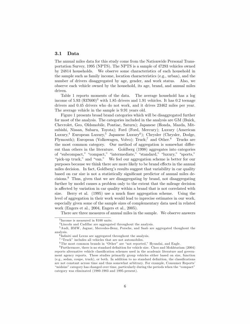
to questions of the form: �About how many miles was this vehicle driven?� Thetime unit is a year if the vehicle was purchased more than a year ago, and it isthe tenure of the car otherwise. In either case, an annualized miles variable iscreated. Also, we observe the odometer reading at the time of the interviewand a few weeks after the interview. Pickrell and Schimek (1999) report resultsusing reported annual miles and imputed annual miles based on the changein the odometer (after adjusting for season, etc.) Their estimates look quitesimilar to each other. Using the odometer reading, we also can construct ameasure of annual miles as a function of age by aggregating vehicles into cellsby age and brand and then di¤erencing the annual miles readings. Figure 2shows how di¤erent estimates of annual miles vary with the age of the vehicle.The estimate based on odometer reading is very imprecise and, in fact, for oldervehicles, is frequently negative. For the remainder of the analysis, we focus onreported annual miles.10

Figure 2 shows a marked decline in annual miles as a function of age.11

This is consistent with previous work (Pickrell and Schimek, 1999). There aremany outliers in the annual miles data, so we checked to see if there are largedi¤erences between mean and median annual miles. While there are some dif-ferences, especially at late ages, these are not substantial enough to warrantusing orthogonal regression methods. One reason for the decline in annualmiles with age is that the vehicle becomes less useful and the household drivesthe vehicle less. Lave (1994) suggests an alternative in which household het-erogeneity causes some households to drive new cars many miles and then sellthem and other households to drive fewer miles and hold the cars longer. Rust(1985) and Hendel and Lizzeri (1999) also have models of household hetero-geneity with similar results. Later, in Section 5, we show that the householde¤ects discussed in these papers are important in understanding the relationshipbetween changes in annual miles and changes in used car prices. In any case,older vehicles are driven less than newer vehicles.We can disaggregate the data by brand and then plot annual miles as a

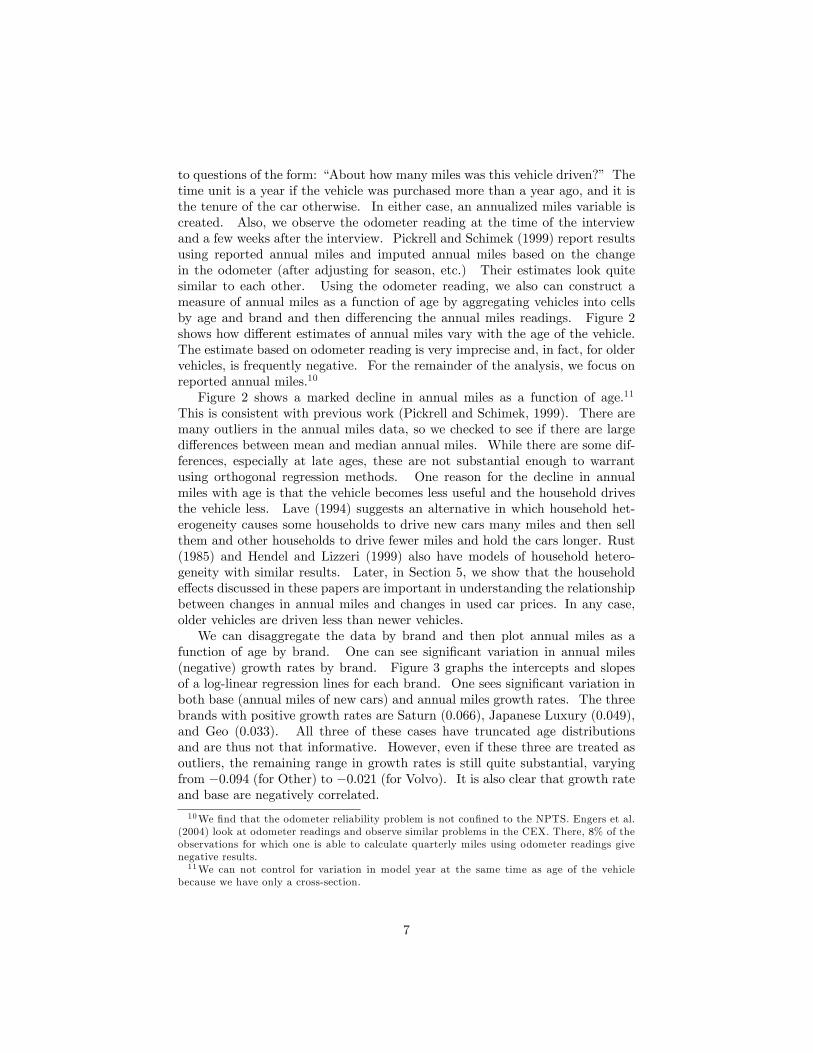
function of age by brand. One can see signi�cant variation in annual miles(negative) growth rates by brand. Figure 3 graphs the intercepts and slopesof a log-linear regression lines for each brand. One sees signi�cant variation inboth base (annual miles of new cars) and annual miles growth rates. The threebrands with positive growth rates are Saturn (0:066), Japanese Luxury (0:049),and Geo (0:033). All three of these cases have truncated age distributionsand are thus not that informative. However, even if these three are treated asoutliers, the remaining range in growth rates is still quite substantial, varyingfrom �0:094 (for Other) to �0:021 (for Volvo). It is also clear that growth rateand base are negatively correlated.

10We �nd that the odometer reliability problem is not con�ned to the NPTS. Engers et al.(2004) look at odometer readings and observe similar problems in the CEX. There, 8% of theobservations for which one is able to calculate quarterly miles using odometer readings givenegative results.11We can not control for variation in model year at the same time as age of the vehicle

because we have only a cross-section.

7

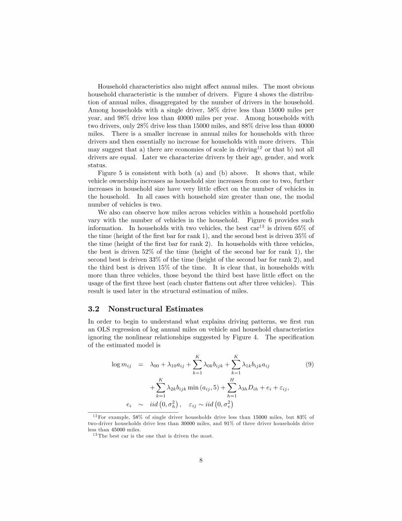
Household characteristics also might a¤ect annual miles. The most obvioushousehold characteristic is the number of drivers. Figure 4 shows the distribu-tion of annual miles, disaggregated by the number of drivers in the household.Among households with a single driver, 58% drive less than 15000 miles peryear, and 98% drive less than 40000 miles per year. Among households withtwo drivers, only 28% drive less than 15000 miles, and 88% drive less than 40000miles. There is a smaller increase in annual miles for households with threedrivers and then essentially no increase for households with more drivers. Thismay suggest that a) there are economies of scale in driving12 or that b) not alldrivers are equal. Later we characterize drivers by their age, gender, and workstatus.Figure 5 is consistent with both (a) and (b) above. It shows that, while

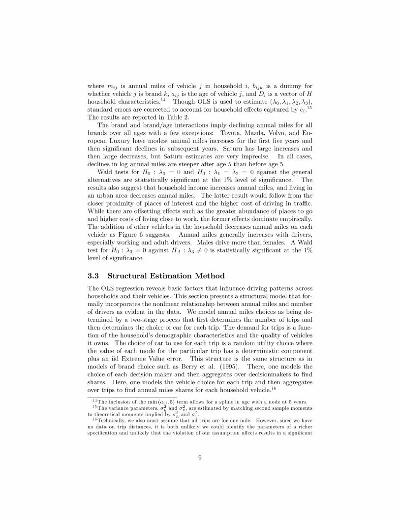
vehicle ownership increases as household size increases from one to two, furtherincreases in household size have very little e¤ect on the number of vehicles inthe household. In all cases with household size greater than one, the modalnumber of vehicles is two.We also can observe how miles across vehicles within a household portfolio

vary with the number of vehicles in the household. Figure 6 provides suchinformation. In households with two vehicles, the best car13 is driven 65% ofthe time (height of the �rst bar for rank 1), and the second best is driven 35% ofthe time (height of the �rst bar for rank 2). In households with three vehicles,the best is driven 52% of the time (height of the second bar for rank 1), thesecond best is driven 33% of the time (height of the second bar for rank 2), andthe third best is driven 15% of the time. It is clear that, in households withmore than three vehicles, those beyond the third best have little e¤ect on theusage of the �rst three best (each cluster �attens out after three vehicles). Thisresult is used later in the structural estimation of miles.

3.2 Nonstructural Estimates

In order to begin to understand what explains driving patterns, we �rst runan OLS regression of log annual miles on vehicle and household characteristicsignoring the nonlinear relationships suggested by Figure 4. The speci�cationof the estimated model is

logmij = �00 + �10aij +KXk=1

�0kbijk +KXk=1

�1kbijkaij (9)

+KXk=1

�2kbijkmin (aij ; 5) +HXh=1

�3hDih + ei + "ij ;

ei � iid�0; �2h

�; "ij � iid

�0; �2v

�12For example, 58% of single driver households drive less than 15000 miles, but 83% of

two-driver households drive less than 30000 miles, and 91% of three driver households driveless than 45000 miles.13The best car is the one that is driven the most.

8

where mij is annual miles of vehicle j in household i, bijk is a dummy forwhether vehicle j is brand k, aij is the age of vehicle j, and Di is a vector of Hhousehold characteristics.14 Though OLS is used to estimate (�0; �1; �2; �3),standard errors are corrected to account for household e¤ects captured by ei.15

The results are reported in Table 2.The brand and brand/age interactions imply declining annual miles for all

brands over all ages with a few exceptions: Toyota, Mazda, Volvo, and Eu-ropean Luxury have modest annual miles increases for the �rst �ve years andthen signi�cant declines in subsequent years. Saturn has large increases andthen large decreases, but Saturn estimates are very imprecise. In all cases,declines in log annual miles are steeper after age 5 than before age 5.Wald tests for H0 : �0 = 0 and H0 : �1 = �2 = 0 against the general

alternatives are statistically signi�cant at the 1% level of signi�cance. Theresults also suggest that household income increases annual miles, and living inan urban area decreases annual miles. The latter result would follow from thecloser proximity of places of interest and the higher cost of driving in tra¢ c.While there are o¤setting e¤ects such as the greater abundance of places to goand higher costs of living close to work, the former e¤ects dominate empirically.The addition of other vehicles in the household decreases annual miles on eachvehicle as Figure 6 suggests. Annual miles generally increases with drivers,especially working and adult drivers. Males drive more than females. A Waldtest for H0 : �3 = 0 against HA : �3 6= 0 is statistically signi�cant at the 1%level of signi�cance.

3.3 Structural Estimation Method

The OLS regression reveals basic factors that in�uence driving patterns acrosshouseholds and their vehicles. This section presents a structural model that for-mally incorporates the nonlinear relationship between annual miles and numberof drivers as evident in the data. We model annual miles choices as being de-termined by a two-stage process that �rst determines the number of trips andthen determines the choice of car for each trip. The demand for trips is a func-tion of the household�s demographic characteristics and the quality of vehiclesit owns. The choice of car to use for each trip is a random utility choice wherethe value of each mode for the particular trip has a deterministic componentplus an iid Extreme Value error. This structure is the same structure as inmodels of brand choice such as Berry et al. (1995). There, one models thechoice of each decision maker and then aggregates over decisionmakers to �ndshares. Here, one models the vehicle choice for each trip and then aggregatesover trips to �nd annual miles shares for each household vehicle.16

14The inclusion of the min (aij ; 5) term allows for a spline in age with a node at 5 years.15The variance parameters, �2h and �

2v , are estimated by matching second sample moments

to theoretical moments implied by �2h and �2v .

16Technically, we also must assume that all trips are for one mile. However, since we haveno data on trip distances, it is both unlikely we could identify the parameters of a richerspeci�cation and unlikely that the violation of our assumption a¤ects results in a signi�cant

9

Let mij be annual miles of car j in household i, j = 1; ::; Ji, and

mi� =

JiXj=1

mij : (10)

Let household i have demographic characteristics Di and car j of household ihave characteristics Cij . We can model

mij = g (j; Ci; ui; �)mi�; (11)

mi� = h (Ci; Di; ui; �)

where Ci = (Ci1; Ci2; ::; CiJi), ui = (ui1; ui2; ::; uiJi) is a vector of errors, ui �iidN

�0; �2uI

�, and � is a vector of parameters speci�ed below. The data suggest

that, even for households with 4 or more cars, the characteristics of only the 3best cars matter in the h function (see Figure 6).17

Let the value of car j be18

Vij = Cij�+ uij ; (12)

and let Ri (j) be the rank of car j in household i according to Vij ; i.e., Ri (j) <Ri (k) i¤ Vij > Vik and Ri (j) 2 f1; 2; ::; Jig.19 Let S (�) be the inverse of Ri (�).We model h semiparametrically using polynomials with imposed monotonic-

ity. In particular, de�ne p0 (v) � 1 and

pj (v) =MXm=1

�jmvm (13)

as an Mth-degree polynomial in v for j > 0. Let

�ViS(j) =

8<: 0 if j = 0ViS(j) if j = 1ViS(j) � ViS(j�1) if j > 1

; (14)

i.e., �ViS(1) is the value of i�s best choice, and �ViS(j) is the negative of themarginal reduction in value between the jth best choice and the (j � 1)th bestchoice for j > 1. De�ne J�i = min (Ji; 3) and

� [J�i ; Vi] =

J�iXj=0

J�iXk=j

�jkpj��ViS(j)

�pk��ViS(k)

�(15)

way.17Figure 4 shows that the marginal e¤ect of drivers after the second driver is small also.

However, we use characteristics of all of the drivers because it is easy to do so and it is notobvious how to rank drivers.18One should note that we do not allow the value of car j to depend upon the household�s

demographics. Berry et al. (1995) found valuation of vehicle characteristics (e.g. miles pergallon, size) varied across income groups, and one might expect these vehicle characteristicsto in�uence how much a vehicle of a particular brand is driven. For instance, Hondas withhigh mpg may be driven over longer distances than Volvos with low mpg. While these aregood arguments, since we use only age and brand as car characteristics, we think it unlikelywe could measure household demographic/car characteristic interactions with any precision.19We ignore ties because they occur with zero probability.

10

as a product of polynomials in di¤erent combinations of �ViS(j) and �ViS(k)with �00 = 0 and �01 = 1. We think of � [J�i ; Vi] as a semiparametric approx-imation of a general function in

��ViS(j)

�3j=0

in the sense that, as the samplesize increases, we can increase M (and also the number of ranked cars in thefunction from 3). This point is formalized in the Appendix.

Note that � [J�i ; Vi] is equivalent to a function in�ViS(j)

�J�ij=0

that can beconstructed by expanding equation (15) and then collecting terms appropriately.The speci�cation in equation (15) is preferred because it makes it easier toimpose conditions such as @� [J�i ; Vi] =@�ViS(j) declining in j.

20 Consider thespecial case where �jk = 0 for all j > 0 and only linear terms (= 1) occur inequation (13); i.e.,

� [J�i ; Vi] =

J�iXk=j

�0k�ViS(k): (16)

Then, for example, if all car values increase by 1, � [J�i ; Vi] increases by 1; and,if just the best car increases in value by one, then � [J�i ; Vi] increases by 1��02.All of the remaining �jm terms in equation (13) and �jk terms in equation(15) allow for nonlinearity. The �jm terms allow �ViS(k) to enter � [J�i ; Vi]nonlinearly, and the �jk terms allow for interactions among the pj

��ViS(j)

�terms.21

We could model h (Ci; Di; ui; �) as a function of � [J�i ; Vi] and Di, but such aspeci�cation would allow for the possibility that � [J�i ; Vi] would have some esti-mated negative partial derivatives. Stern (1996) found that, without imposingmonotonicity on a semiparametric function of two arguments that theory im-plied should be monotone, the estimated function deviated far from a monotonefunction. Mukarjee and Stern (1994) and Stern (1996) suggest a simple methodto impose monotonicity, similar in spirit to Matzkin (1991), and we use an anal-ogous method here. For any function f :W ! R whereW is a nonempty subsetof RJ for some J , de�ne

[f ] (x) = supy�x

[f (y)] : (17)

transforms the function f into a new function [f ] that is nondecreasing inall of its arguments. In fact,

[f ] � g (18)

for all nondecreasing g such that f � g. We use the [�] transformation becauseannual miles by household should be increasing in the vector of V values. Wemodel

log h (Ci; Di; ui; �) = [�] +Di (19)

20We specify equation (19) in terms of �ViS(j) rather than ViS(j) also because the opti-mization method performs signi�cantly better. This speci�cation implies that �ViS(j) � 0for all j > 1.21Some terms are not identi�ed separately; e.g. the linear term in � and the linear term in

�.

11

as a partial linear equation, �exible in car values and linear in household charac-teristics. We approximate the function by discretizing the V -space and thenchecking for monotonicity in h point by point. This sounds computationallyintensive, but, in fact, its cost is proportional to the number of grid points.We assume that the g function depends on Ci and ui only through the e¤ect

of Ci and ui on Vi = (Vi1; Vi2; ::; ViJi), and it depends on j only through Vij andRij = Ri (j). Let

g (j; Ci; ui; �) =exp f (Vij ; Rij ; �)gPj0 exp f (Vij0 ; Rij0 ; �)g

(20)

where

(Vij ; Rij ; �) =

( PJi�1k=Rij

!k�ViS(k) � ViS(k+1)

�if Rij � Ji � 1

0 if Rij = Ji(21)

is a spline function (in slopes) in Vij with nodes at the values of the ranked Vi�s.This is a weighted logit function that allows for �exibility with respect to howranking interacts with car value. Note that it is increasing in each element ofVi (assuming !k is positive 8k) and that, if !k = 1 8k, then g (j; Ci; ui; �) isa logit function. While there is no explicit �outside option� in equation (20),we allow for an outside option by modelling the total demand for annual milesin equation (19). Finally, the functional forms of equations (19) through (21)satisfy the conditions described in Berry et al. (1995) for a unique solution inui to the set of equations,

mij

mi�= g (j; Ci; ui; �) ; j = 1; 2; ::; Ji; (22)

logmi� = log h (Ci; Di; ui; �) : (23)

De�ne bui as the value of ui that satis�es equations (22) and (23). If we decom-pose bui into bui1 and bui=1 = (bui2; bui3; ::; buiJi), then, conditional on any value ofui1 = u0i1, there is a unique solution u

0i=1 to equation (22). Furthermore,

@u0ij@u0i1

= 1 for all j (24)

because of the usual location identi�cation problem in random utility models.The value of bui1 is the value that solves equation (23).We ignore endogeneity problems. In particular, households that require a

lot of annual miles (large ui) will purchase vehicles of greater quality (largerVij). More importantly, households that like to drive (large ui) may also liketo have higher quality vehicles (larger Vij) independent of their need for annualmiles.22 Thus, the estimates of � in equation (13) may be biased upwards.

22Verboven (2002) models the choice of car make, focusing on whether to buy a car witha gas or diesel engine, given desired annual miles of the household. While we ignore theendogeneity of brand choice, he ignores the endogeneity of annual miles.

12

Given the nature of the data, all we can do here is acknowledge the problemand interpret results with caution.23

The set of parameters to estimate is � =��; ; �; �; !; �2u

�where � is the

e¤ect of car characteristics Cij on car values Vij in equation (12), is the e¤ectof demographic characteristics Di on total household annual miles in equation(19), � is the set of polynomial coe¢ cients in equation (13), � is the set ofweights on each of the polynomial products used to determine the total value ofthe household�s car portfolio in equation (15), ! is the set of weights determininghow car shares depend upon relative values in equations (20) and (21), and �2u isthe variance of the unobserved household heterogeneity in equation (12). Thelog likelihood contribution of family i is

Li =

JiXj=1

log1

�u�

�buij (Ci; �)�u

�� log j� (�)j (25)

where � [�] is the standard normal density function and � (�) is the Jacobian.Our model speci�cation di¤ers signi�cantly from other models of demand

for annual miles. For example, Goldberg (1998) uses a model similar to Du-bin and McFadden (1984) to measure the joint decision of buying a new carand how many miles to drive it. The technology available in Dubin and Mc-Fadden (1984) controls for the selection bias in annual miles associated withbrand choice. As stated above, we ignore this selection bias. On the otherhand, while we have a rich speci�cation of how annual miles decisions for eachcar in a household�s portfolio interact, Goldberg includes only aggregate char-acteristics of the household�s portfolio (average stock age, age of newest car,whether any other cars are owned, and number of cars) and estimates a milesequation for only the new car recently purchased.24 Mannering and Winston(1985) construct a dynamic model of car choice and utilization but also do notreally allow for any interaction across cars within a household in simultaneousdecisions about how much to use each car.25

3.4 Results for Structural Speci�cation

We estimate a number of di¤erent speci�cations of the structural model of thehousehold�s decision of how much to drive each vehicle it owns. The speci�-23We cannot use the methodology developed in Verboven (2002) because our problem is

more complicated. In particular, Verboven (2002) assumes each household owns only onecar. While this assumption re�ects European household vehicle stock in the early 1990s,the sample period for this study, a quarter of western European households now own twoor more vehicles (Ingham, 2002). This assumption is further violated in the U.S. wherethe average household owns 1.91 vehicles. Because we are using U.S. data and Verboven�smethodology relies heavily on the one vehicle per household assumption, we had to developanother methodology to examine household annual miles decisions.24Our model suggests that Goldberg�s aggregated portfolio characteristics could never be a

su¢ cient statistic for all of the characteristics of the portfolio. For example, while the numberof cars matters, it must be interacted with some measure of the quality of each of the cars.25 In their model, the use of a car today a¤ects the use of similar cars in the future because

it a¤ects perceptions of the car. However, there is no decision today about how to allocatedriving miles among cars in the household portfolio.

13

cation we focus on, reported in Table 3, restricts � in equation (13) to linearfunctions26 and the higher order shape parameters (� in equation (19))27 andreports estimates for ! in equation (21), car characteristic e¤ects (� in equation(12)), demographic e¤ects ( in equation (19)), and log �u in equation (12).28

This allows for the value of each vehicle to in�uence log household annual miles�exibly. We allow (in �) for brand e¤ects and brand-age interaction e¤ectsas we did in the nonstructural model. Most of the estimates are statisticallysigni�cant, and almost all of the brand-age e¤ects are negative after adding theage slope e¤ects.Many of the estimates in Table 3 are di¢ cult to interpret. Starting with the

! shape parameters in equation (21), recall that the number of annual milesdriven on a given vehicle depends on its value relative to the other vehiclesowned. Thus, !k captures how the relative value of the kth car to the next bestvehicle a¤ects the multinomial logit share of household miles driven on thatvehicle. Consider a family with three vehicles. The log ratio of the model�schoice probability for the choice with the best V to a multinomial logit model�schoice probability for the choice with the best V is displayed in Figure 7 fordi¤erent values of �Vi2 and �Vi3. The log ratios are always positive becauseb!2 > !1 = 1; this implies that values for third choices (or lower) receive lessweight than values for the second choice. In particular, we can write theprobability of the �rst choice as

P1 =exp f!1V1 + (!2 � !1)V2g

exp f!1V1 + (!2 � !1)V2g+ exp f!2V2g+ exp f!2V3g(26)

which converges to a multinomial logit probability as !2 ! !1 and is greaterthan the multinomial logit probability when !2 > !1. Also note that the choiceprobabilities given our speci�cation still have the independence of irrelevantalternatives property (after conditioning on u), so Figure 7 displays also the logratio probabilities for the second best choice.The � coe¢ cients in equation (15) capture how the (total) household annual

miles is dependent on the nonlinear relationships between the relative valuesof di¤erent combinations of vehicles from which the household takes on trips.Since we estimated only linear terms, the h (�) is linear as well.The results we are most interested in are the age e¤ects. When interpreting

the age e¤ects on the annual miles decision, consider that, for the most valuable

26 �j1 = 1 and �j2 = 0 for j = 1; 2; 3:27�00 = 1 and �01 = 1 (for identi�cation), �jk = 0 8j 6= 0; �1 = 1, �k = 0 8k 6= 1.28We estimate a third speci�cation adding the nonlinear � terms and �nd that it behaves

very poorly. It is clear that adding such terms leads to severe over�tting of the data as iscommon in using polynomials to approximate functional form.

14

car in a household portfolio,29

@ logmij

@Ageij=

�[1� g (j; Ci; ui; �)] +

1

h (Ci; Di; ui; �)

�(�Age + �Brand-Age) ;

(27)while, for the second most valuable car,

@ logmij

@Ageij=

�[1� g (j; Ci; ui; �)] (!2 � 1) +

�02h (Ci; Di; ui; �)

�(�Age + �Brand-Age)

(28)(note that b!2�1 = 0:456 and b�02 = 1:931). However, since �Age does not varyover brands (b�Age = �0:302 if Age � 5 and b�Age = �0:337 if Age > 5), onecan compare variation in age e¤ects over brands by focusing just on the Brand-Age estimates. One should note that the thought experiment correspondingto @ logmij

@Ageijis not to let the car age one year; rather it is to sell the car and

purchase a car of the same brand one year older. The importance of this pointbecomes clear in Section 5.Probably, a more fruitful way to understand age derivatives in the structural

speci�cation is to directly evaluate and graph average derivatives of log annualmiles with respect to age. Such derivatives vary by brand, age, household-carportfolios, and household characteristics. In Figure 8, we aggregate over house-holds, therefore averaging over household-car portfolio and household charac-teristics e¤ects. Figure 8 shows how average derivatives for a selected subset ofbrands vary with brand and age. The average derivatives are mostly negativeand declining with age. Of those not represented in Figure 8, only Dodge haspositive age derivatives; the other 16 are all negative and declining with age.We also can measure how the usage of other cars in the family changes as a

particular car ages. The implication of the vehicle annual miles share functionin equation (20) is that, as a particular car ages (holding all else constant), itbecomes less valuable (because the relevant estimated total � e¤ects are gen-erally negative), thus increasing the shares of the other cars in the household�sportfolio. On the other hand, the household total miles function in equation(19) implies that total household miles decline. The structural estimates implythat the net e¤ect is very small and negative, averaging about �0:4% per year.We also can measure how demographic characteristics a¤ect car usage. The

estimates in Table 3 measure in equation (19), the e¤ect of demographiccharacteristics on total miles. We do not interact demographic characteristicswith car characteristics. Thus, the demographic derivatives do not vary overcars or over age. The results also suggest that vehicle utilization varies acrosshouseholds with varying numbers of drivers. Annual miles rises with the numberof adult drivers, male drivers, and working drivers in the household, but falls

29Note that, for multinomial logit probabilities,

@ logP

@A=P (1� P )

P

@P

@A= (1� P ) @P

@A:

15

with other types of drivers. Finally, household income increases annual miles,but unlike with the OLS estimates, living in an urban area raises annual miles.

4 Prices

In the previous section, we show that annual miles falls as a vehicle ages. Beforewe can ascertain the relationship between annual miles and prices, we explorethe extent to which scrappage rates explain price declines. We jointly estimateused car prices and scrappage rates as a vehicle ages. Then we examine if weneed to correct for a selection bias; poorer quality vehicles are scrapped �rstbiasing the estimates of price declines.

4.1 Data

The price data for this study come from the Kelley Blue Books over the period1986 - 2000.30 The price data are generated from sales reports to the NationalAutomobile Dealer�s Association (NADA) provided by member dealers. Foreach year in the sample period, we observe the average price of each brand ofcar for each relevant manufacturing year.31 For example, in 1990, we observethe average price of multiple models for each brand for the 15 model yearsfrom 1986 - 1990 inclusive. We observe 8887 prices and 7918 changes in price.The mean price is $10797, and the standard deviation is $8463. The pricerange is from $825 to $97875. The average change in log prices is �0:133, andits standard deviation is 0:077. One can see in Figure 9 that there is a largepercentage price decline in the �rst year and then smaller declines in subsequentyears. When vehicles reach 12 years of age, price declines signi�cantly diminish.We argue below that this can be explained by a scrapping e¤ect. Table 4 showshow price changes vary by brand.32 There is signi�cant variation by brandwith Honda and Toyota having the smallest average price declines and Isuzuand Hyundai having the largest average price declines. American cars tend tohave larger than average price declines.Finally, the scrapping data used in this study are from R.L. Polk & Co. The

scrapping rates are observed reductions in the stock of cars of each brand as aproportion of the stock the year before. We observe scrapping rates only for

30See Porter and Sattler (1999) for a more detailed discussion of the quality of the Blue Bookdata. Alternatively, one could use transaction prices to capture car-speci�c quality. However,these transaction prices also re�ect the relative bargaining power of the buyer and seller andother characteristics idiosyncratic to the particular car. If we were to uses transactions prices,we would average them just as Kelly Blue Book did to average out any car-speci�c e¤ects.31Prices based on the base model, four-door sedan model are used whenever possible. When

matching the price data with the vehicle data in the NPTS, we assume all cars are sold atthe base model price. Thus, we lose some variation in prices within a brand-model, but docapture the variation in prices across brand-models.32The truck category was dropped because we lack price data. NADA records price infor-

mation for trucks in a separate publication from the one that reports passenger vehicle pricesused for this study. The other category was also dropped and the Isuzu and Hyundai brandswere added in place because we had detailed price information on cars in this category.

16

eight car categories and only for a limited number of relevant vintages.33 So weuse nearby substitutes for other brands and use scrapping rates for cars manu-factured in 1990. Also, we ignore the �rst two years of the car because observedscrapping rates are actually negative as car dealers sell their remaining stock.The substitution pattern is reported in Table 5. One might worry that scrap-ping rates are not constant over time and thus it is problematic to use scrappingrates for cars manufactured in just 1990 to proxy for all scrapping rates. How-ever, we have no data on scrapping rates disaggregated over both calendar timeand brands. Also data from Ward�s Communications (2001), shown in Figure10, show that, once after initial volatility in scrapping rates (across calendartime), scrapping rates are relatively stable. Most of the selection e¤ect occursat these later ages.

4.2 Pricing Estimation Method

Given the data described above, we can estimate a pricing function for passengervehicles controlling for scrappage. Assume the price of car j of brand i at age tis

pijt = �it + �ij (29)

�ij � iidN�0; �2

�(30)

with�it = �i + �it: (31)

Let pit be the average observed price of brand i cars at age t, and let dit be thescrapping rate of brand i cars at age t. Scrapping occurs because some fractiond� are totaled or otherwise exogenously disappear and because some cars havenonpositive value. We observe only positive prices; cars with negative pricesare junked. The joint moments of (pit; dit) are

Epit =

1�p2�

R1��it

(�it + �) expn� �2

2�2

od�

1�p2�

R1��it

expn� �2

2�2

od�

= �it + ����it�

����it�

� ; (32)

Edit = d� +

1�p2�

R ��it��it�1

expn� �2

2�2

od�

1�p2�

R1��it�1

expn� �2

2�2

od�= d� +

���it�1

�

�� �

��it�

����it�1

�

� :

In the data, we observe fpi1; pi2; ::; piT gni=1 and fdi1; di2; ::; diT gni=1 for some

subset of n car brands. Let yit = (pit; dit)0, let � = (�; �; �; d�) be the set of

parameters, and consider minimizing the objective function,

L (�) =1

nT

Xi;t

(yit � Eyit)0 (yit � Eyit) : (33)

33The Polk scrapping rate data were given to us by Matthew Shum.

17

The asymptotic distribution of the estimates ispnT�b� � �� � N (0;) (34)

with

= B�1plim

24 1

nT

Xi;t

@E�yit j b��@�0

� (35)

E�(yit � E (yit j �)) (yit � E (yit j �))0 j �

�0@E

�yit j b��@�

35B�1where

B = plim1

nT

Xi;t

@E (yit j ��)@�0

@E (yit j �)

@�: (36)

4.3 Pricing and Scrappage Results

The pricing and scrappage parameter estimates are reported in Table 6.34 Allof the estimates are highly signi�cant. The most important parameters are theestimates of � and d�. The estimate of log � is 1:345 implying an estimate of� of 3:838. While we think this may be a bit high, it is necessary to explainthe curvature in the price curve and the increase in scrapping rates as cars age.The estimate of d� is 0:0091. The estimate of d� is very close to the observedscrapping rates of four year old cars. This is what should be expected.One can perform a residual analysis to see how well the model �ts the data.

De�ne

edit = dit � E�dit j b�� ; (37)

epit = pit � E�pit j b�� :

Table 7 reports average residuals for scrapping rates and prices aggregated bybrand, and Table 8 reports the same aggregated by age. Though most ofthe average residuals are statistically signi�cant, most are small in magnitude.Note that, for brand-speci�c residuals, almost all of the brands have averagescrapping rate residuals and price residuals of the same sign. In cases wherethis is not so, then the pricing parameters (�i; �i) can adjust to reduce the ab-solute value of both residuals. The residual analysis suggests that Nissan,Volvo,34Additional brands were dropped because we do not have scrappage rates on their close

substitutes to estimate the joint moments of (pit; dit). Those dropped were the three luxurybrands, Geo, Hyundai, Saturn. Alternatively, one could estimate a hazard function for vehiclescrappage. Chen and Niemeier (2005) estimate retention rates by vehicle class (all passengervehicles were in the same class). They use smog check data collected by the California Bureauof Automotive Repair. But because vehicles under age 5 are exempt from inspection, a fullhazard function cannot be estimated for our purposes.

18

Honda, and Dodge are bad �ts.35 Part of what may be occurring, especially forNissan, Honda, and Volvo, is that manufacturers signi�cantly change their carsacross model years during the sample period leading to di¤erent prices pathsacross model years (or sets of model years). For example, the 3rd generationHonda Accord arrived in 1986, and Accords were upgraded when the 4th gen-eration Accord arrived in 1990. Thus, there may be di¤erent price paths forpre and post 1990 Honda Accords. Because of this, a composition e¤ect maybe contaminating our results for these brands. It also suggests that our modelis not rich enough to explain the nonlinearity in observed average pricing andits interaction with scrapping rates. In particular, we overestimate scrappingrates at ages t � 12. This is partly true because used car prices depend onmany factors not controlled for in this study such as the vehicle�s equipmentand condition. While these factors in�uence actual transaction prices, they donot a¤ect the Kelly Blue Book value. This value is just a starting point fordealers to estimate a vehicles�worth and does not take into account car-speci�cfactors. Thus, controlling for additional factors would not improve the model�spredictive power of Kelly used car prices across vehicle age.Lastly, we examine if one must correct our results for a selection bias. Used

car prices represent the average price of automobiles still in use in time t andnot the average price of vehicles in the original cohort. Failing to control for thescrapping of poorer quality vehicles �rst would bias upwards the rate of declinein prices. In order to compare how alternative speci�cations �t the data, we canplot the observed price path, the predicted price path ignoring selection, andthe predicted price path taking into account selection. For example, the pricepaths for Oldsmobiles are shown in Figure 11.36 For most brands, our modelis very precise in predicting the price paths after controlling for the selectionbias. However, there is something about the price paths for Honda, Volvo, andVolkswagen that we miss. In particular, we cannot explain increasing pricepaths with our selection model when the underlying randomness is normal.We also can plot scrapping paths.37 We can not explain nonmonotone scrap-

ping rates and, in general, we miss the scrapping rates by signi�cant amounts.This occurs basically because the terms in in equation (33) associated withedit and e

pit in equation (37) gives more weight to e

pit than e

dit.

35This also may be due to not controlling for how the market perceives changes in vehiclemodels. Purohit (1992) shows that if the market perceives a new model is less preferable thanearlier models, then the demand for used versions of these vehicle rises, increasing their usedprices (and vice versa). These shifts in the price paths would not be captured by our model.36Price paths for each brand are available at

http://faculty.virginia.edu/stevenstern/resint/empiostf/selection_gi¢ les/paths.html.

37Scrapping paths for each brand are available also at

http://faculty.virginia.edu/stevenstern/resint/empiostf/selection_gi¢ les/paths.html.

19

5 Relationship Between Annual Miles and Price

Now that we have estimated the process that generates both annual miles andpricing, we can investigate the relationship between these two processes. Theestimates of � from equation (9) in Table 2 tell us how log annual miles declineswith age, disaggregated by brand, and the estimates of � from equation (31) inTable 6 tell us how log prices decline with age, disaggregated by brand.38 Wecan compare annual miles and price decline estimates to see if the two processesare moving together. This is done in Figure 12. The OLS estimates of thelinear relationship between them are

b�j = �0:791 + 6:75b�j + uj : (38)

The t-statistic on the b�j coe¢ cient is 2:00, and the R2 is 0:21. This, along withthe price/maintenance results in Engers et al. (2004), suggests that declines inannual miles might explain declines in price as a car ages.Consider using the structural average derivatives with respect to age, some of

which are shown in Figure 8, to explain the change in log prices. The estimatedslope is 0:557, and R2 = 0:020. So the obvious question is why the OLS esti-mates explain prices pretty well and the structural estimates do not. The answeris that the two sets of estimates are measuring very di¤erent objects. In partic-ular, the structural estimates are measuring @ logMiles

@Age jDemographics,Portfolios ; i.e.,unlike the OLS estimates, they are holding constant demographic e¤ects andhousehold-car portfolio e¤ects. We can interpret these di¤erences in light of themodel of car turnover in Rust (1985) or the base model in Hendel and Lizzeri(1999) (with no transactions costs or asymmetric information problems). Inthese models, because there are no transactions costs or asymmetric informationproblems, each household sells its cars every period. Changes in prices as thecar ages re�ect both @ logMiles

@Age jDemographics,Portfolios and the changes due to themovement of cars to di¤erent household types as the car ages.We would like to measure the demographic e¤ects and household-car portfo-

lio e¤ects but do not have enough data to estimate models of portfolio choice.39

However, we can construct semiparametric estimates of total average derivatives(allowing demographic characteristics and household-car portfolios to change).Using our structural estimates, we construct an estimate of the total derivativefor each car j in household i in our sample. Let bij be the brand of car j inhousehold i and aij be its age. De�ne �ij = Dib (from equation (19)) as apropensity score for household demographic characteristics in the spirit of Ru-bin (1979), Rosenbaum and Rubin (1983), and Heckman et al. (1998) and � as

38Since we aggregate car makes in the NPTS and Kelley Blue Book data the same way,we have no problem matching annual miles slope estimates from Table 2 with price slopeestimates from Table 6.39The fact that the NPTS is not a panel prevents us from measuring changes in portfolios.

20

a bandwidth.40 Then our estimate of the total derivative is

d@ logMilesij@Age

=

Pi0j0 1 (bi0j0 = bij) 1 (ai0j0 = aij + 1)K

��i0��i�

�logmi0j0P

i0j0 1 (bi0j0 = bij) 1 (ai0j0 = aij + 1)K��i0��i�

� �logmij

(39)where 1 (�) is the indicator function and K (�) is a kernel function. Note that wecondition on cars having the same brand and being one year older. We use twoseparate kernel functions. First, we setK (�) � 1. This choice of kernel functioncauses averaging over varying demographic characteristics of households owningcars of brand bij with age equal to aij+1. Then we setK (�) equal to a standardnormal density function truncated at �4. This choice of kernel function controlsfor household demographics; i.e., we weight more heavily the annual miles ofcars i0j0 in households with similar demographic characteristics Di0 to householdi�s characteristics Di (where similarity is measured in terms of the propensityscores).Using the estimates from equation (39), we construct median derivatives

disaggregated by brand and disaggregated by brand and age. We use me-dian derivatives because mean derivatives are unduly in�uenced by outliers. Infact, Figure 13 shows how median derivatives, disaggregated by age, vary overage. The three di¤erent derivatives shown are: 1) �Age�plots the derivativeholding demographic characteristics and portfolio choices constant, 2) �Total�plots the derivative holding only demographic characteristics constant, while3) �No Demographics�plots the derivative when both demographic character-istics and vehicle portfolio are allowed to change. Note that, while the �Age�curve behaves well, the other two curves are poorly behaved. Curves for otherbrands look similar. Figure 14 presents the distribution function of derivatives(censored at �0:5) for Chrysler aggregated over age (other brands have similargraphs). While there is some mass in between the censoring points (in factthe median is always strictly between the censoring points), most of the massis beyond the censoring points.The plim of an OLS estimate in the presence of measurement error in the

explanatory variable is ��2x=��2x + �

2e

�where � is the true value of the linear

slope term, �2x is the sample variance of the explanatory variable, and �2e is the

variance of the measurement error.41 Under the assumption that a sample ofrandom variables is iid, the standard deviation of the estimate of a median is[2pnf (�)]

�1 where n is the number of observations used to estimate the medianand f (�) is the density of the random variables evaluated at the median (e.g.,Bickel and Doksum, 1977, p. 400). The estimated standard deviations of themedian estimates and corresponding bias ratios (�2x=

��2x + �

2e

�) are listed in

Table 9. The estimated median partial derivative @ logMiles@Age jDemographics,Portfoliosis measured very precisely relative to the variation across brands �x. But theestimates of the total derivatives have large standard deviations.

40We use one quarter of the standard deviation of the propensity score as the bandwidth.41 In the more general case where there is heteroskedasticity in the measurement error across

observations (as is true here), the term �2e is replaced by n�1P�2ei.

21

Figures 13 and 14 and Table 9 suggest that the derivatives estimated usingequation (39) are problematic. However, we proceed to use them in a regres-sion similar to equation (38). We do this partially because there is no betteralternative and partially because, even though the biases of the OLS estimatesare large, the R2 statistics (and therefore t-statistics and F -statistics) have noasymptotic bias.42 The results are presented in Table 10. The �rst row of Table10 repeats the results of equation (38), and the second row repeats the resultsusing the partial derivatives already discussed. The last two rows correspond tousing K (�) equal the truncated normal density and K (�) � 1 respectively. Thepartial derivatives @ logMiles@Age jDemographics,Portfolios have no explanatory power forprice changes. For the linear semiparametric speci�cation, the partial derivativeis negative, casting more doubt on the credibility of the linear semiparametricestimates. On the other hand, the total derivative @ logMiles

@Age and the derivative

controlling for demographics @ logMiles@Age jDemographics both explain price changes

as well as the OLS equation from Figure 12.43 When we further consider thatthe implication of Figure 14 is that median derivatives are measured with sig-ni�cant error (and we know that measurement error in an explanatory variablecauses bias towards zero), we conclude that the structural estimates explainthe price changes better than the OLS equation. These results suggest thatportfolio e¤ects and turnover e¤ects in the spirit of Rust (1985) and Hendel andLizzeri (1990) are important in explaining price changes as cars age.The results also demonstrate the value of the structural estimates. While

the OLS estimates in equation (38) provide a useful measure of the total e¤ectof aging on car prices, they can not be used to decompose the aging e¤ect intoits components: the direct aging e¤ect, the household-car portfolio e¤ect, andthe household demographics (or car turnover) e¤ects. The structural estimates,along with information about the distribution of cars across households, allowus to decompose the e¤ects.

42This result is not as well known as the bias result. However, given the linear model,

y = x�+ u

with

w = x+ e;

y = wb+ v;

R2 =(wb)0 (wb) =n

y0y=n=b0 (x+ e)0 (x+ e) b=n

(x� + u)0 (x� + u) =n

and

plimR2 =�2�2x�2x + �

2e

�2x + �2e

�2�2x + �2u

=�2�2x

�2�2x + �2u

which is independent of measurement error in x.43Note that multiplying the reported estimates for the total derivative and the derivative

controlling for demographics by the inverse of the associated bias terms in Table 9 results inan estimate very similar to the OLS derivatives.

22

6 Conclusion

The objective of this paper is to determine if changes in a vehicle�s net bene�ts,proxied by annual miles, explain the observed decline in used car prices overthe vehicle�s life. We �rst model the household-vehicle annual miles decisionusing two alternative models. The OLS model restricts the relationship betweenannual miles and household demographics to be linear. The structural modelconstructed allows for a nonlinear relationship as exhibited in the data. We thencompare the two models and �nd the structural model of household mileagedecisions better explains the observed price decline in used car prices.The intuition behind the dominance of the structural model is that it for-

malizes the link between annual miles choices and household and vehicle-stockcharacteristics. The model speci�cation allows for car portfolios and householddemographic characteristics to in�uence how vehicle age a¤ects annual miles.We �nd that the observed decline in used car prices as a vehicle ages is bestexplained by decomposing the age e¤ect into three components: the direct aginge¤ect, the household-car portfolio e¤ect, and the household demographics (orcar turnover) e¤ect. This implies that the e¤ect age has on annual miles (andconsequently the vehicle�s value) cannot be estimated independently of house-hold characteristics and household-car portfolio choices. The intuition behindthis result is that, as a vehicle becomes older and less reliable, households areless likely to take that vehicle on long driving trips. When possible, householdsoften take instead the newer, more reliable vehicle on those trips. The declinein usage (and subsequently annual miles) continues until the �nal years of avehicle�s working life where it one day primarily becomes used to transport theowner on short local trips. The estimated relationship between annual milesand vehicle value is consistent with the theoretical model of car turnover inRust (1995) or the base model in Hendel and Lizzeri (1999) (with no transac-tion costs or asymmetric information problems). Portfolio and turnover e¤ectsexplain price changes as a car ages.The literature provides alternative explanations for the decline in prices:

adverse selection, declining quality, and higher maintenance costs. Quality andmaintenance costs both a¤ect the net bene�t �ow as discussed in Section 2.While asymmetric information has been shown (empirically) to lower prices,Engers et al. (2004) shows that this can not be the case for maintenance costs.Thus, we are left with two competing explanations for the observed decline:adverse selection and quality deterioration.Hendel and Lizzeri (1999) provides an empirical test to determine if informa-

tion asymmetry or exogenous depreciation (in vehicle bene�ts) is the dominantfactor that drives price declines in the used car market. Ideally, one would liketo separate out and measure each factor�s e¤ect on price declines individually.However, in order to separate these two e¤ects, researchers must have a betterunderstanding of how quality depreciates over the vehicle�s life and how thistranslates to explaining the observed decline in used car prices as a vehicle ages.Many of these issues have been addressed in this paper. Separation of these twocompeting explanations for price declines is left for future work.

23

Our results also are relevant for policy makers who need to estimate traveldemand to identify driving patterns or combat congestion for instance. Weidentify the factors that determine household driving behavior. We also showthat one can not estimate annual miles just as a function of the vehicle�s age andbrand, but one also must factor in how household demographics and householdportfolio choices in�uence driving decisions.

7 Appendix: Denseness of Polynomial Approx-imations

Take any vector x 2 Rn. We do a two-step change of variables, �rst arrangingthe components of x in descending order, and then taking di¤erences. Thevector y = R(x); the reordering of x in descending order, consists of the samecomponents as x but in non-increasing order, so that y1 � y2 � ::: � yi� ::: � yn and y = (x�(1); x�(2); :::; x�(n)) where � is a permutation on the setf1; 2; :::; ng. If there are ties, the permutation � is not unique, but this does notlead to a nonuniqueness in y = R(x). By de�nition, the value of a symmetricfunction f is unaltered by a permutation of its arguments, and so, for all x,f(x) = f(R(x)) = f(y).Given real numbers a < b, any symmetric function on the box B = [a; b]n �

Rn is completely determined by its values on the wedge

W = R(B) = fy 2 B : y1 � y2 � ::: � yi � ::: � yng: (40)

There is a one-to-one correspondence between the continuous symmetric func-tions on B and the continuous functions on W , and this one-to-one corre-spondence is clearly an isometry. Thus approximating a continuous symmetricfunction on B is equivalent to approximating a continuous function on W .Next we introduce the transformation � that di¤erences any vector in W .

Each vector y 2 W maps to a vector z = �(y) = (y1; y2 � y1; y3 � y2; :::; yn �yn�1), and it is easy to check that the mapping � is one-to-one and onto thecompact set

D = �(W ) = fz 2 [a; b]� [a� b; 0]n�1 :nXj=1

zj 2 [a; b]g: (41)

Since, for each i, yi =Pi

j=1 zj , each polynomial in the yi can be written as apolynomial in the associated zi. Conversely, since each zi is a linear combinationof at most two yi, each polynomial in the zi can be written as a polynomial inthe associated yi. Since � and its inverse are linear, it is a homeomorphismbetween W and D:We show that any continuous symmetric function on the boxB is the uniform

limit of a sequence of polynomials onW when the composite change of variablez = � � R (x) is applied to the x vector. Any symmetric function on B iscompletely determined by its values on W . Via the homeomorphism �, eachcontinuous function on W is associated with a continuous function on D.

24

Proposition 1 Any continuous symmetric function f(x) on B can be uniformlyapproximated by a sequence of polynomials in z = � �R(x).

Proof. We apply the Stone-Weierstrass approximation theorem (see Rudin,1976), which states that any algebra of functions on a compact set that vanishesnowhere and separates points is dense (in the uniform norm) in the space ofcontinuous functions on that set. The set of all polynomials on the compact setD is an algebra since the sum and product of polynomials are polynomials as arescalar multiples of polynomials. Because (nonzero) constants are polynomials,the algebra of polynomials never vanishes at any point of D, and, given any twodistinct points z0; z00 in D, it is possible to �nd polynomials that take di¤eentvalues at the two points (just �nd an index i such that z0i 6= z00i , and then thelinear polynomial zi su¢ ces). So the algebra of polynomials separates points.

By the Stone-Weierstrass Theorem, the polynomials on D are dense in thespace of continuous functions on D:with the uniform norm. Thus any continu-ous function on D is the uniform limit of polynomials in D.

8 References

References

[1] Alberini A, Harrington W, McConnell V. 1995. Determinants of participa-tion in accelerated vehicle retirement programs. Rand Journal of Economics26: 93-112. DOI:10.2307/2556037

[2] Alberini A, Harrington W, McConnell W. 1998. Fleet turnover and old carscrap policies. Resources for the Future. Discussion Paper 98-23.

[3] Berry S, Levinsohn J, Pakes A. 1995. Automobile prices in market equilib-rium. Econometrica. 63: 841-890. DOI:10.2307/2171802

[4] Bickel P, Doksum K. 1977. Mathematical Statistics: Basic Ideas and Se-lected Topics. Holden-Day, Inc: San Francisco, Cal.

[5] Chen C, Niemeier D. 2005. A mass point vehicle scrappage model. Trans-portation Research Part B. 39: 401-415. DOI:10.1016/j.trb.2004.06.003

[6] Choo S, Mokhtarian P. 2004. What type of vehicle do people drive? the roleof attitude and lifestyle in in�uencing vehicle type choice. TransportationResearch Part A. 38:201-222.

[7] Dubin J, McFadden D. 1984. An econometric analysis of residen-tial appliance holdings and consumption. Econometrica. 52: 345-362.DOI:10.2307/1911493

[8] Engers M, Hartmann M, Stern S. 2004. Automobile maintenance costs,used cars, and adverse selection.�University of Virginia manuscript.

25

[9] Engers M, Hartmann M, Stern S. 2005. Are lemons really hot potatoes?�University of Virginia manuscript.

[10] Fabel O, Lehmann E. 2002. Adverse selection and market substitution byelectronic trade.� International Journal of the Economics of Business. 9:175-193. DOI:10.1080/13571510210134646

[11] Genesove D. 1993. Adverse selection in the wholesale used car market.Journal of Political Economy. 101: 644-665. DOI:10.1086/261891

[12] Goldberg P. 1998. The e¤ects of the corporate average fuel e¢ ciencystandards in the US. Journal of Industrial Economics. 46: 1-33.DOI:10.1111/1467-6451.00059

[13] Heckman J, Ichimura H, Todd P. 1998. Matching as an economet-ric evaluation estimator. Review of Economic Studies. 65: 261-294.DOI:10.1111/1467-937X.00044

[14] Hendel I, Lizzeri L. 1999. Adverse selection in durable goods markets.American Economic Review. 89: 1097-1114.

[15] Ingham R. 2002. Europe takes lead in tackling the car. Agence France-Presse. September 20.

[16] Lave C. 1994. What really matters is the growth rate of vehicle miles trav-eled. Presented at the 72nd Annual Meeting of the Transportation ResearchBoard. Washington, D.C.

[17] Mannering F, Whinston C. 1985. A dynamic empirical analysis of householdvehicle ownership and utilization. Rand Journal of Economics. 16: 215-236.DOI:10.2307/2555411

[18] Matzkin R. 1991. Semiparametric estimation of monotone and concave util-ity functions for polychotomous choice models. Econometrica. 59: 1315-1327. DOI:10.2307/2938369

[19] Mukarjee H, Stern S. 1994. Feasible nonparametric estimation of multiargu-ment monotone functions. Journal of the American Statistical Association.89: 77-80. DOI:10.2307/2291202

[20] Pickrell D, Schimek S. 1999. Growth in motor vehicle ownership and use:evidence from the nationwide personal transportation survey. Journal ofTransportation and Statistics. 2: 1-17.

[21] Porter R, Sattler P. 1999. Patterns of trade in the market for used durables:theory and evidence.�NBER Working Paper 7149.

[22] Purohit D. 1992. Exploring the relationship between the markets for newand used durable goods: the case of automobiles. Marketing Science. 11:154-167.

26

[23] Rosenbaum P, Rubin D. 1983. The central role of the propensityscore in observational studies for causal e¤ects. Biometrika. 70: 41-55.DOI:10.1093/biomet/70.1.41

[24] Rubin D. 1979. Using multivariate matched sampling and regression ad-justment to control bias in observational studies. Journal of the AmericanStatistical Association. 74: 318-329. DOI:10.2307/2286330

[25] Rudin W. 1976. Principles of Mathematical Analysis. 3rd ed. McGraw-Hill:NY.

[26] Rust J. 1985. Stationary equilibrium in a market for durable assets. Econo-metrica. 53: 783-805. DOI:10.2307/1912654

[27] Stern S. 1996. Semiparametric estimates of the supply and demand e¤ectsof disability on labor force participation. Journal of Econometrics. 71: 49-70. DOI: 10.1016/0304-4076(94)01694-1

[28] Verboven F. 2002. Large quality-based price discrimination and tax inci-dence: evidence from gasoline and diesel cars. Rand Journal of Economics.33: 275-297. DOI:10.2307/3087434

[29] Walls M, Krupnick A, Hood HC. 1993. Estimating the demand for ve-hicle miles traveled using household survey data: results from the 1990nationwide personal transportation survey. Discussion Paper ENR93-25.Resources for the Future. Washington, D.C.

[30] Ward�s Communications. 2001. Ward�s Automotive Yearbook. South�eld,MI.

27

9 Tables and Figures

Table 1Sample Moments

Variable Mean Std Dev Variable Mean Std DevHousehold Characteristics # Worker Drivers 1.40 0.86log (Income) 5.93 0.70 # Vehicles 1.91 0.82Urban 0.61 0.49 Annual Miles (100) 234.62 172.89# Drivers 1.85 0.72# Adult Drivers 1.65 0.62 Vehicle Characteristics# Male Drivers 0.92 0.54 Age 9.91 5.97

Notes:

1. The number of households is 24814, and the number of vehicles is 47293.

2. Income is measured in $100 units.

3. Annual Miles is measured in 100 mile units.

===========================================

28

Table 2log Mileage OLS Regression Estimates

Vehicle CharacteristicsBrand Dummy (�0k) Age (�1k) min [Age,5] (�2k)

Constant (�00; �10)4.595**(0.078)

-0.099**(0.006)

Chrysler-0.312**(0.132)

0.003(0.013)

0.080**(0.038)

Dodge-0.268**(0.101)

0.006(0.009)

0.067**(0.024)

Plymouth-0.437**(0.151)

0.008(0.011)

0.106**(0.036)

Ford-0.284**(0.079)

0.032**(0.007)

0.045**(0.014)

Mercury-0.389**(0.109)

0.028**(0.010)

0.070**(0.027)

Buick-0.202**(0.108)

0.054**(0.009)

-0.011(0.023)

Chevrolet-0.303**(0.084)

0.031**(0.007)

0.049**(0.016)

Oldsmobile-0.305**(0.110)

0.041**(0.008)

0.042*(0.025)

Pontiac-0.368**(0.095)

0.028**(0.008)

0.058**(0.022)

Saturn-0.400**(0.122)

-0.715(0.988)

0.877(0.993)

American Luxury-0.316**(0.120)

0.031**(0.009)

0.064**(0.029)

Japanese Luxury-0.538(0.192)

0.084(0.342)

0.059(0.365)

European Luxury-0.539**(0.193)

0.020**(0.009)

0.130**(0.034)

Honda-0.381**(0.085)

0.055**(0.010)

0.057**(0.021)

Mitsubishi-0.222(0.154)

0.058(0.044)

0.028(0.073)

Mazda-0.438**(0.133)

0.055**(0.017)

0.054(0.041)

Nissan-0.299**(0.100)

0.029**(0.011)

0.056**(0.027)

Subaru-0.099(0.148)

0.019(0.018)

0.041(0.047)

Toyota-0.380**(0.091)

0.045(0.010)

0.053**(0.022)

Volkswagen-0.275*(0.163)

0.033**(0.009)

0.065*(0.038)

29

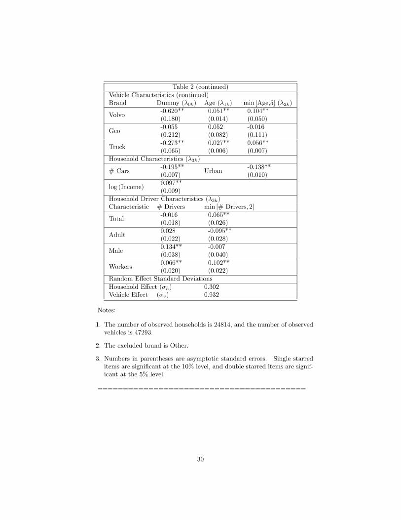
Table 2 (continued)Vehicle Characteristics (continued)Brand Dummy (�0k) Age (�1k) min [Age,5] (�2k)

Volvo-0.620**(0.180)

0.051**(0.014)

0.104**(0.050)

Geo-0.055(0.212)

0.052(0.082)

-0.016(0.111)

Truck-0.273**(0.065)

0.027**(0.006)

0.056**(0.007)

Household Characteristics (�3k)

# Cars-0.195**(0.007)

Urban-0.138**(0.010)

log (Income)0.097**(0.009)

Household Driver Characteristics (�3k)Characteristic # Drivers min [# Drivers; 2]

Total-0.016(0.018)

0.065**(0.026)

Adult0.028(0.022)

-0.095**(0.028)

Male0.134**(0.038)

-0.007(0.040)

Workers0.066**(0.020)

0.102**(0.022)

Random E¤ect Standard DeviationsHousehold E¤ect (�h) 0.302Vehicle E¤ect (�v) 0.932

Notes:

1. The number of observed households is 24814, and the number of observedvehicles is 47293.

2. The excluded brand is Other.

3. Numbers in parentheses are asymptotic standard errors. Single starreditems are signi�cant at the 10% level, and double starred items are signif-icant at the 5% level.

=========================================

30

Table 3Structural Estimates

Brand Variables Intercept Age Slope Brand Variables Intercept Age Slope

Chrysler-0.101**(0.006)

0.164**(0.017)

European Luxury-0.329**(0.016)

0.447**(0.013)

Dodge-0.307**(0.002)

0.392**(0.011)

Honda0.161**(0.001)

0.054**(0.002)

Plymouth0.064**(0.001)

-0.158**(0.011)

Mitsubishi-0.433**(0.028)

-0.027(0.051)

Ford-0.124**(0.001)

0.361**(0.000)

Mazda-0.202**(0.011)

-0.189**(0.010)

Mercury0.051**(0.013)

-0.076**(0.003)

Nissan0.186**(0.001)

0.063**(0.002)

Buick-0.038**(0.007)

0.120**(0.008)

Subaru-0.067*(0.035)

0.022(0.041)

Chevrolet0.251**(0.001)

-0.096**(0.002)

Toyota-0.032**(0.002)

0.256**(0.002)

Oldsmobile-0.073**(0.001)

0.130**(0.008)

Volkswagen-0.076**(0.017)

0.215**(0.001)

Pontiac-0.059**(0.008)

-0.066**(0.000)

Volvo0.106**(0.033)

-0.045(0.031)

Saturn-0.032**(0.003)

-0.206(0.027)

Geo0.584**(0.020)

0.273**(0.031)

American Luxury0.387**(0.003)

-0.052**(0.000)

Other0.119**(0.005)

0.032(0.007)

Japanese Luxury0.131**(0.012)

-0.028(0.116)

Truck-0.078**(0.000)

0.227**(0.002)

Table 3 (continued)Other Variables

Constant3.985**(0.040)

# Drivers-0.070**(0.012)

Age-0.337**(0.000)

# Adult Drivers0.134**(0.011)

min (Age; 5)0.035**(0.000)

# Male Drivers0.311**(0.012)

log (Household Income)0.220**(0.007)

# Working Drivers0.034**(0.008)

Urban0.093**(0.011)

log �u-0.969**(0.002)

log Likelihood -64967.4

31

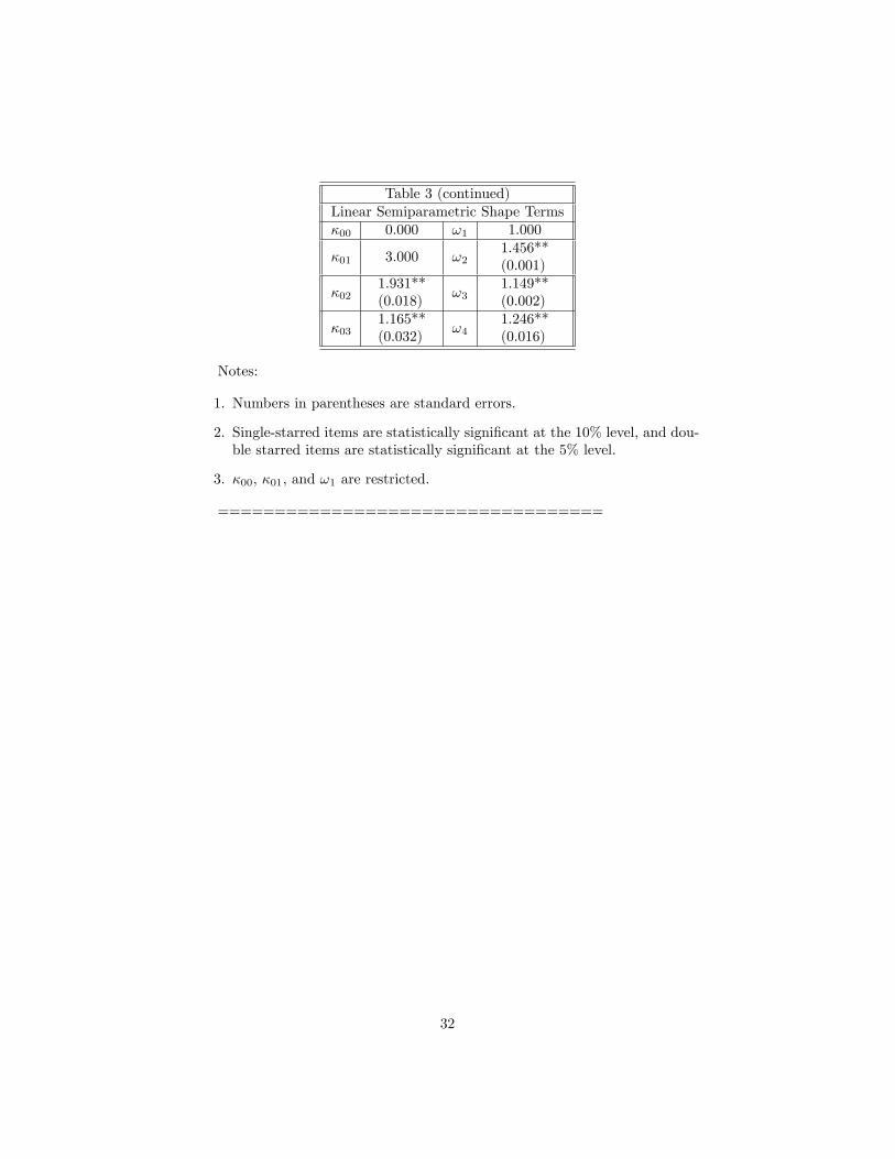
Table 3 (continued)Linear Semiparametric Shape Terms�00 0.000 !1 1.000

�01 3.000 !21.456**(0.001)

�021.931**(0.018)

!31.149**(0.002)

�031.165**(0.032)

!41.246**(0.016)

Notes:

1. Numbers in parentheses are standard errors.

2. Single-starred items are statistically signi�cant at the 10% level, and dou-ble starred items are statistically signi�cant at the 5% level.

3. �00, �01, and !1 are restricted.

==================================

32

Table 4Moments of Change in Log Prices by Brand

Variable # Obs Moments Variable # Obs Moments

Isuzu 96-0.176**(0.133)

JapaneseLuxury

156-0.133(0.064)

Chrysler 282-0.146**(0.072)

EuropeanLuxury

659-0.131(0.070)

Dodge 360-0.139(0.076)

Honda 441-0.097**(0.068)

Plymouth 274-0.135(0.085)

Mitsubishi 181-0.141(0.103)

Ford 692-0.136(0.071)

Mazda 354-0.120**(0.077)

Mercury 338-0.148**(0.066)

Nissan 395-0.118**(0.068)

Buick 474-0.145**(0.065)

Subaru 197-0.130(0.099)

Chevrolet 675-0.135(0.079)

Toyota 543-0.105**(0.064)

Oldsmobile 297-0.145**(0.066)

Volkswagen 121-0.106**(0.061)

Pontiac 503-0.133(0.066)

Volvo 191-0.114**(0.079)

Saturn 80-0.121(0.073)

Geo 65-0.182**(0.130)

AmericanLuxury

427-0.165**(0.067)

Hyundai 117-0.182**(0.121)

Notes:

1. Numbers in parentheses are standard deviations.

2. Double-starred items are statistically signi�cant at the 5% level for H0 :� logP = �0:133 vs HA : � logP 6= �0:133 (assuming observations areiid within a brand).

==================================

33

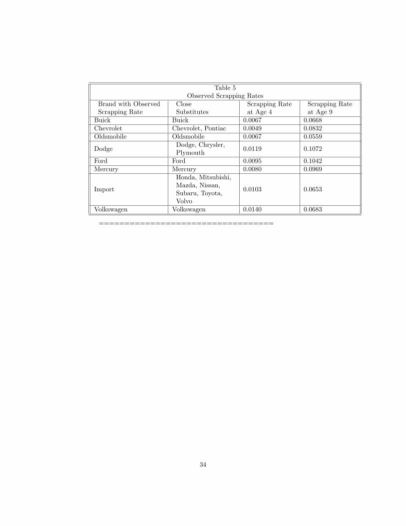
Table 5Observed Scrapping Rates

Brand with ObservedScrapping Rate

CloseSubstitutes

Scrapping Rateat Age 4

Scrapping Rateat Age 9

Buick Buick 0.0067 0.0668Chevrolet Chevrolet, Pontiac 0.0049 0.0832Oldsmobile Oldsmobile 0.0067 0.0559

DodgeDodge, Chrysler,Plymouth

0.0119 0.1072

Ford Ford 0.0095 0.1042Mercury Mercury 0.0080 0.0969

Import

Honda, Mitsubishi,Mazda, Nissan,Subaru, Toyota,Volvo

0.0103 0.0653

Volkswagen Volkswagen 0.0140 0.0683

==================================

34

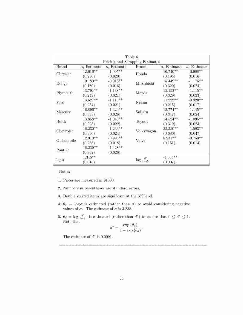
Table 6Pricing and Scrapping Estimates

Brand �i Estimate �i Estimate Brand �i Estimate �i Estimate

Chrysler12.616**(0.230)

-1.095**(0.020)

Honda10.740**(0.195)

-0.908**(0.016)

Dodge10.189**(0.180)

-0.916**(0.016)

Mitsubishi15.449**(0.320)

-1.175**(0.024)

Plymouth13.791**(0.249)

-1.138**(0.021)

Mazda15.152**(0.329)

-1.115**(0.023)

Ford13.627**(0.254)

-1.115**(0.021)

Nissan11.222**(0.215)

-0.920**(0.017)

Mercury16.896**(0.333)

-1.324**(0.026)

Subaru15.774**(0.347)

-1.145**(0.024)

Buick13.858**(0.298)

-1.043**(0.022)

Toyota14.524**(0.319)

-1.095**(0.023)

Chevrolet16.230**(0.330)

-1.233**(0.024)

Volkswagon22.350**(0.680)

-1.593**(0.047)

Oldsmobile12.910**(0.236)

-0.995**(0.018)

Volvo8.231**(0.151)

-0.753**(0.014)

Pontiac16.239**(0.302)

-1.428**(0.026)

log �1.345**(0.018)

log d�

1�d�-4.685**(0.007)

Notes:

1. Prices are measured in $1000.

2. Numbers in parentheses are standard errors.

3. Double starred items are signi�cant at the 5% level.

4. �� = log � is estimated (rather than �) to avoid considering negativevalues of �. The estimate of � is 3:838.

5. �d = log d�

1�d� is estimated (rather than d�) to ensure that 0 � d� � 1.

Note that

d� =exp f�dg

1 + exp f�dg:

The estimate of d� is 0:0091.

================================================

35

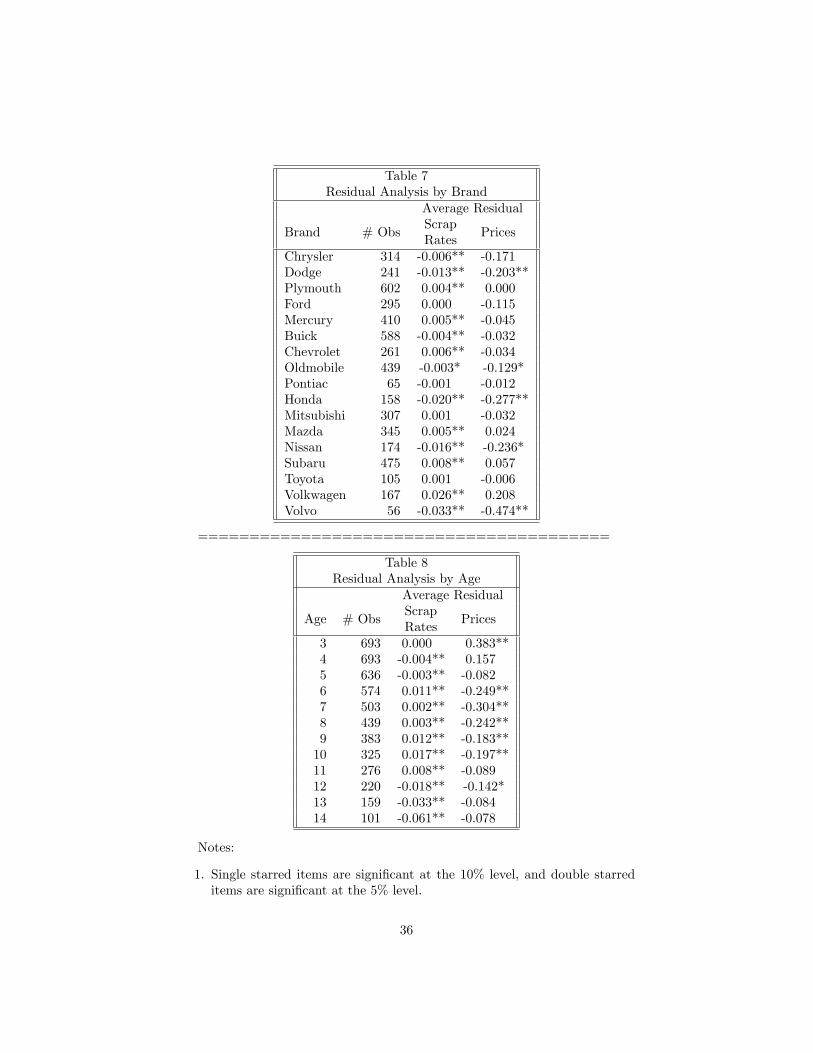
Table 7Residual Analysis by Brand

Average Residual

Brand # ObsScrapRates

Prices

Chrysler 314 -0.006** -0.171Dodge 241 -0.013** -0.203**Plymouth 602 0.004** 0.000Ford 295 0.000 -0.115Mercury 410 0.005** -0.045Buick 588 -0.004** -0.032Chevrolet 261 0.006** -0.034Oldmobile 439 -0.003* -0.129*Pontiac 65 -0.001 -0.012Honda 158 -0.020** -0.277**Mitsubishi 307 0.001 -0.032Mazda 345 0.005** 0.024Nissan 174 -0.016** -0.236*Subaru 475 0.008** 0.057Toyota 105 0.001 -0.006Volkwagen 167 0.026** 0.208Volvo 56 -0.033** -0.474**

========================================

Table 8Residual Analysis by Age

Average Residual

Age # ObsScrapRates

Prices

3 693 0.000 0.383**4 693 -0.004** 0.1575 636 -0.003** -0.0826 574 0.011** -0.249**7 503 0.002** -0.304**8 439 0.003** -0.242**9 383 0.012** -0.183**10 325 0.017** -0.197**11 276 0.008** -0.08912 220 -0.018** -0.142*13 159 -0.033** -0.08414 101 -0.061** -0.078

Notes:

1. Single starred items are signi�cant at the 10% level, and double starreditems are signi�cant at the 5% level.

36

========================================

Table 9Measurement Error for Parametric Speci�cation

Explanatory Variable Name �e �x�2x

�2x+�2e

@ logMiles@Age jDemographics,Portfolios Age 22.62 165.53 0.982

@ logMiles@Age jDemographics No Demographics 678.95 280.45 0.146

@ logMiles@Age Total 439.80 283.15 0.293

Note: All standard deviations are multiplied by 10000.========================================

Table 10Linear Relationships Between � logMiles and � logPriceExplanatoryVariable

Estimate

� logMiles (OLS)6.754[0.210]

@ logMiles@Age jDemographics,Portfolios

0.559[0.019]

@ logMiles@Age jDemographics

2.848**[0.196]

@ logMiles@Age

2.957**[0.200]

Notes:

1. Numbers in brackets are R2 statistics.

2. Double-starred items are signi�cant at the 5% level.

========================================

37

Figure 1: Brand Proportions

Figure 1

38

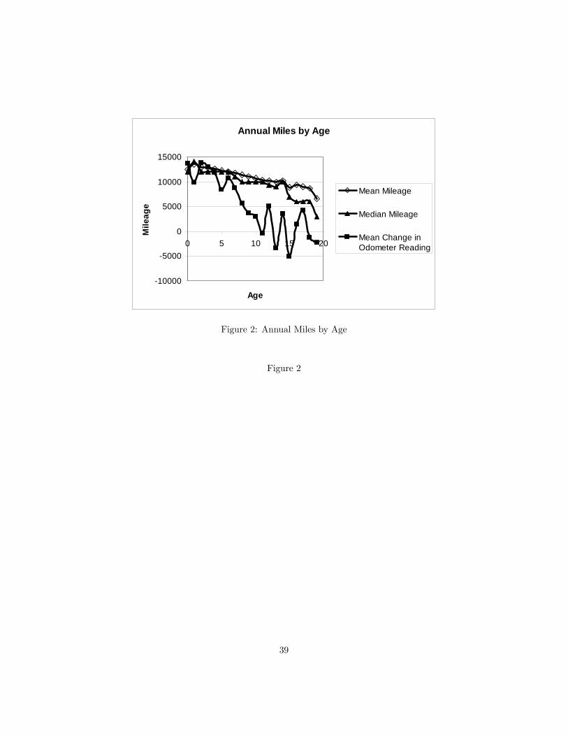
Annual Miles by Age

­10000

­5000

0

5000

10000

15000

0 5 10 15 20

Age

Mile

age

Mean Mileage

Median Mileage

Mean Change inOdometer Reading

Figure 2: Annual Miles by Age

Figure 2

39

Figure 3: Base and Growth Combinations

Figure 3

40

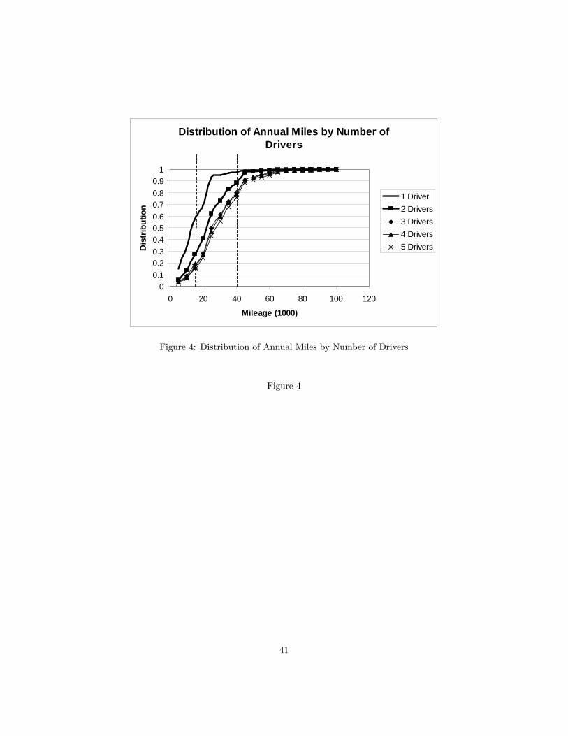
Distribution of Annual Miles by Number ofDrivers

00.10.20.30.40.50.60.70.80.9

1

0 20 40 60 80 100 120

Mileage (1000)

Dis

trib

utio

n

1 Driver2 Drivers3 Drivers4 Drivers5 Drivers

Figure 4: Distribution of Annual Miles by Number of Drivers

Figure 4

41

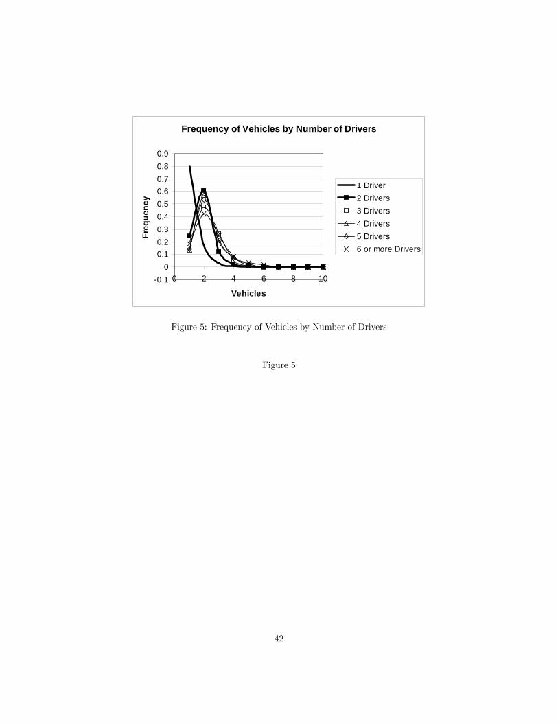
Frequency of Vehicles by Number of Drivers

­0.10

0.10.20.30.40.50.60.70.80.9

0 2 4 6 8 10

Vehicles

Freq

uenc

y

1 Driver2 Drivers3 Drivers4 Drivers5 Drivers6 or more Drivers

Figure 5: Frequency of Vehicles by Number of Drivers

Figure 5

42

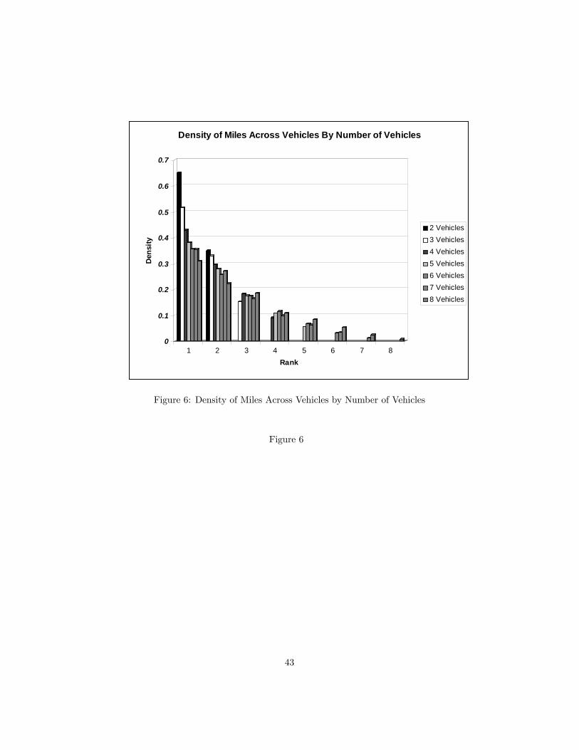
0

0.1

0.2

0.3

0.4

0.5

0.6

0.7D

ensi

ty

1 2 3 4 5 6 7 8Rank

Density of Miles Across Vehicles By Number of Vehicles

2 Vehicles3 Vehicles4 Vehicles5 Vehicles6 Vehicles7 Vehicles8 Vehicles

Figure 6: Density of Miles Across Vehicles by Number of Vehicles

Figure 6

43

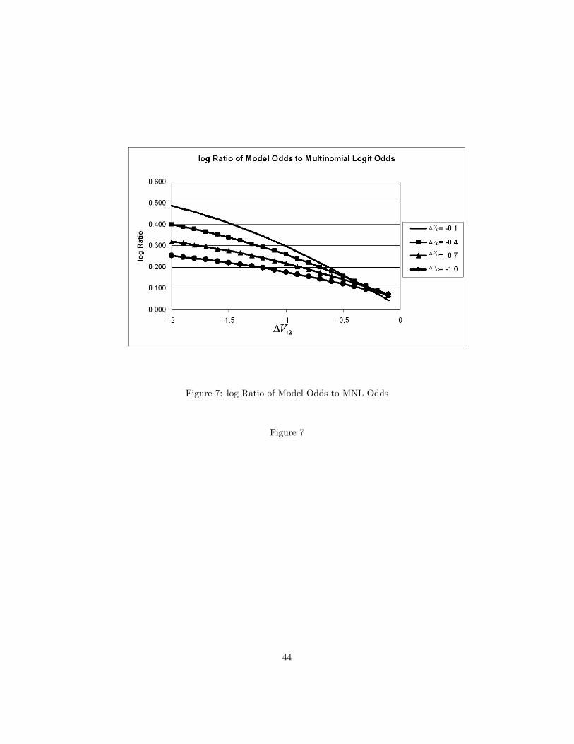
Figure 7: log Ratio of Model Odds to MNL Odds

Figure 7

44

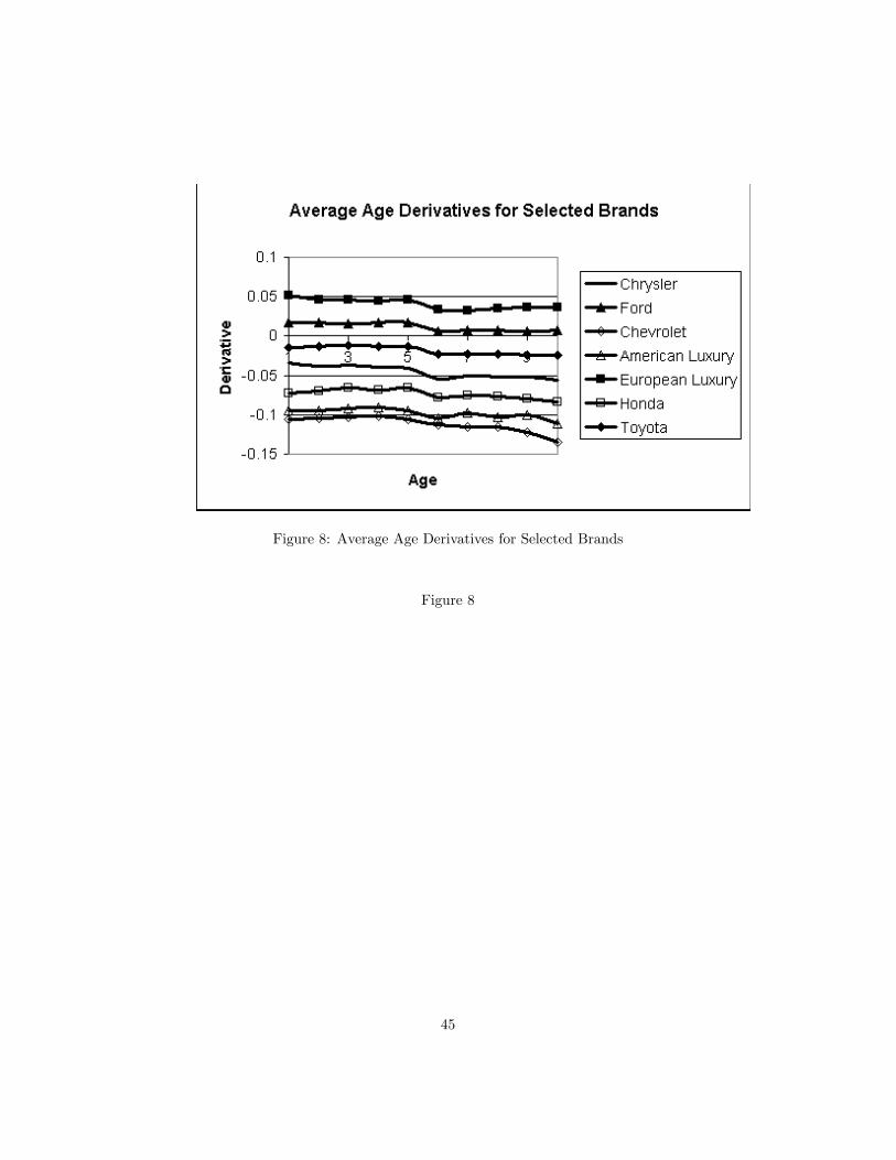
Figure 8: Average Age Derivatives for Selected Brands

Figure 8

45

Figure 9: Change in log Price by Age

Figure 9

46

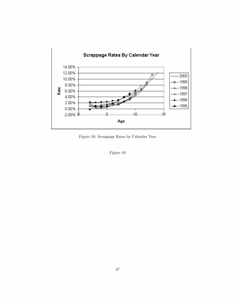
Figure 10: Scrappage Rates by Calendar Year

Figure 10

47

Figure 11: Price Paths for Oldsmobile

Figure 11

48

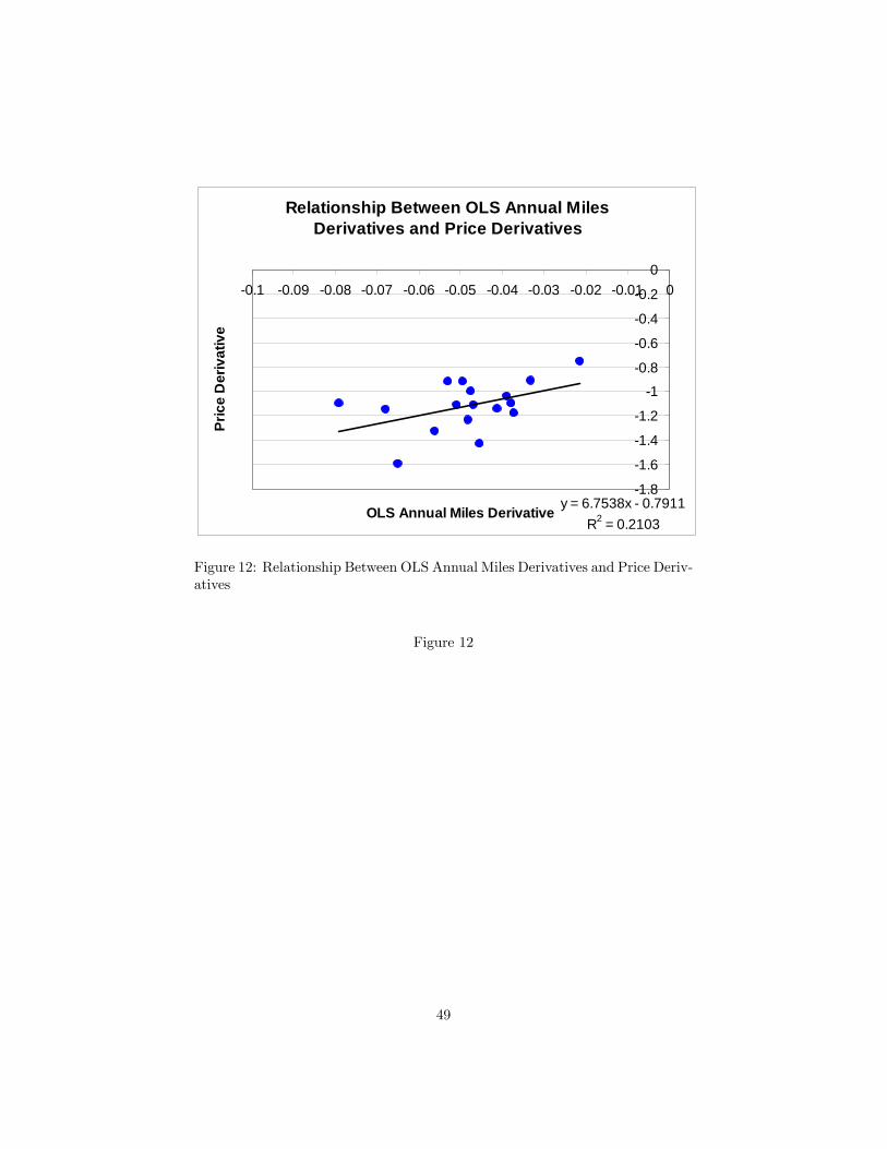
Relationship Between OLS Annual MilesDerivatives and Price Derivatives

y = 6.7538x ­ 0.7911R2 = 0.2103

­1.8

­1.6

­1.4

­1.2

­1

­0.8

­0.6

­0.4

­0.2

0­0.1 ­0.09 ­0.08 ­0.07 ­0.06 ­0.05 ­0.04 ­0.03 ­0.02 ­0.01 0

OLS Annual Miles Derivative

Pric

e D

eriv

ativ

e

Figure 12: Relationship Between OLS Annual Miles Derivatives and Price Deriv-atives

Figure 12

49

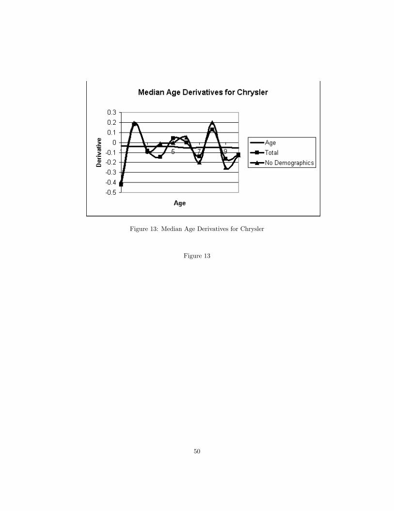
Figure 13: Median Age Derivatives for Chrysler

Figure 13

50

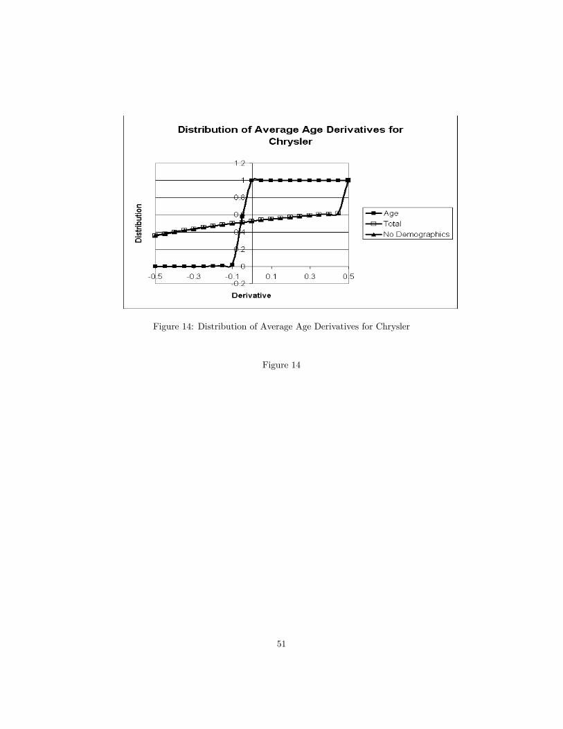
Figure 14: Distribution of Average Age Derivatives for Chrysler

Figure 14

51