PNNL-14072

Annual Report: Remotely Operated NDE System for Inspection of Hanford’s Waste Tank Knuckle Regions and Development of a Small Roving Annulus Inspection Vehicle T-SAFT Scanning Bridge for Savannah River Site Applications A.F. Pardini J.M. Alzheimer S.L. Crawford K.L. Gervais R.V. Harris M.A. Maynard T.J. Samuel J.C. Tucker R.A. Roberts September 2002 Prepared for the U.S. Department of Energy under Contract DE-AC06-76RL01830

DISCLAIMER This report was prepared as an account of work sponsored by an agency of the United States Government. Neither the United States Government nor any agency thereof, nor Battelle Memorial Institute, nor any of their employees, makes any warranty, express or implied, or assumes any legal liability or responsibility for the accuracy, completeness, or usefulness of any information, apparatus, product, or process disclosed, or represents that its use would not infringe privately owned rights. Reference herein to any specific commercial product, process, or service by trade name, trademark, manufacturer, or otherwise does not necessarily constitute or imply its endorsement, recommendation, or favoring by the United States Government or any agency thereof, or Battelle Memorial Institute. The views and opinions of authors expressed herein do not necessarily state or reflect those of the United States Government or any agency thereof. PACIFIC NORTHWEST NATIONAL LABORATORY operated by BATTELLE for the UNITED STATES DEPARTMENT OF ENERGY under Contract DE-AC06-76RL01830 Printed in the United States of America Available to DOE and DOE contractors from the Office of Scientific and Technical Information, P.O. Box 62, Oak Ridge, TN 37831-0062; ph: (865) 576-8401 fax: (865) 576-5728 email: reports@adonis.osti.gov Available to the public from the National Technical Information Service, U.S. Department of Commerce, 5285 Port Royal Rd., Springfield, VA 22161 ph: (800) 553-6847 fax: (703) 605-6900 email: orders@ntis.fedworld.gov online ordering: http://www.ntis.gov/ordering.htm

This document was printed on recycled paper.

(8/00)

PNNL-14072

Annual Report

Remotely Operated NDE System for Inspection of Hanford’s Waste Tank Knuckle Regions and Development of a Small Roving Annulus Inspection Vehicle T-SAFT Scanning Bridge for Savannah River Site Applications AF Pardini JM Alzheimer SL Crawford KL Gervais RV Harris MA Maynard TJ Samuel JC Tucker RA Roberts(a) September 2002 Prepared for the U.S. Department of Energy under Contract DE-AC06-76RL01830 Pacific Northwest National Laboratory Richland, Washington 99352 _____________ (a) Center for NDE at Iowa State University

iii

Summary There is a need to examine the knuckle region of Hanford’s and Savannah River’s double shell tanks (DSTs). Commercial, off-the-shelf systems to examine the knuckle are not available. Preliminary tests at the Pacific Northwest National Laboratory (PNNL) in FY 1999 indicated that a unique technology utilizing ultrasonics could provide a solution to the knuckle examination problem. In FY 2000 PNNL embarked on a study to provide evidence that the ultrasonic technology had the capability to detect and size stress corrosion cracks in the knuckle region of the DSTs. In FY 2001 PNNL designed and fabricated a prototype system, known as the Remotely Operated Nondestructive Examination (RONDE) system, which is capable of examining the knuckle region of the DSTs. At the end of FY 2001, PNNL demonstrated the prototype system. In FY 2002, PNNL concentrated on enhancing the prototype system and completing acceptance testing, equipment qualification, and performance demonstration testing. Also in FY2002, PNNL designed and fabricated a SAFT scanning bridge for the Savannah River Site. In support of the FY02 testing and performance demonstration of the RONDE system, a cracked knuckle mockup was fabricated. Intergranular stress corrosion cracks (IGSCC) were grown in plate material and fabricated into a mockup. This mockup proved invaluable in supporting the performance testing. Equipment qualification and performance testing of the RONDE system have been completed. All required defects in all of the mockups including the IGSCC mockup were readily detected. The NDE Level III Ultrasonic inspector assigned to this project sized all of the detected flaws in the knuckle region of both the sawcut and IGSCC mockups. The sizing results are shown below: Machined Defects Sizing The accuracy requirement for depth sizing of machined defects is a root mean square (RMS) value of 2.54 mm (0.1 in.). The graph below is a plot of the data provided by NDE Level III Ultrasonic inspector Mr. Wes Nelson.

Wes Nelson Sawcuts

0

0.2

0.4

0.6

0 0.5 1

UT Measured Data

True

Sta

te D

ata

PerfectPerformance

UT MeasuredData

iv

Mr. Nelson’s RMS value for all machined defects is 1.4 mm (0.055 in.), well below the 2.54 mm (0.1 in.) criteria. Inter-Granular Stress Corrosion Cracks (IGSCC) The requirement for sizing IGSCC is the same as the requirement for the machined defects, namely 2.54 mm (0.1 in.). The graph shown below is the plot of the data provided by Mr. Nelson.

Wes Nelson Cracks

0

0.2

0.4

0.6

0.8

0 0.2 0.4 0.6 0.8

UT Measured Data

Truc

e St

ate

Dat

a

UT Measured Data

PerfectPerformance

The RMS value of this data is 1.8 mm (0.07 in.), which is well within the 2.54 mm (0.1 in.) requirements. The work described in this report was funded and supported by the U.S. Department of Energy's (DOE) Tanks Focus Area (TFA) Safety program under the coordination of Mike Terry. The TFA provides science and technology solutions to safely and efficiently remediate waste stored in underground storage tanks at five DOE sites.

v

Acknowledgments This work is funded by the Office of Science and Technology within the Energy's Office of Environmental Management under the Tanks Focus Area Program, Technical Task Plan RL37C131. The authors would like to acknowledge the contributions of Mr. Stan Pitman who developed the methodology for cracking the plates used in the IGSCC Mockup; Mr. Wes Nelson, COGEMA Level III who assisted in the performance testing; and Mr. Mike Terry, Tanks Focus Area Safety Technical Integration Manager.

vii

Contents Summary ........................................................................................................................................ iii Machined Defects Sizing............................................................................................................. iii Inter-Granular Stress Corrosion Cracks (IGSCC) ....................................................................... iv Acknowledgments.............................................................................................................................. v 1.0 Introduction ............................................................................................................................... 1.1 2.0 Requirements ............................................................................................................................. 2.1 3.0 Technology Background............................................................................................................ 3.1 3.1 SAFT Technology ............................................................................................................. 3.1 3.2 T-SAFT Technology ......................................................................................................... 3.2 3.3 Signal Parameters.............................................................................................................. 3.3 4.0 Mockups Used for RONDE Qualification and SRAIV Development ...................................... 4.1 4.1 Sawcut Mockup................................................................................................................. 4.1 4.2 EDM Mockup.................................................................................................................... 4.2 4.3 IGSCC Mockup................................................................................................................. 4.2 5.0 RONDE and SRAIV Mechanical Design.................................................................................. 5.1 5.1 Magnetic Wheel Vehicle ................................................................................................... 5.2 5.2 SAFT Bridge ..................................................................................................................... 5.3 6.0 RONDE and SRAIV Control System........................................................................................ 6.1 6.1 SRAIV-SAFT Control....................................................................................................... 6.2 6.2 Tank Top Electronics ........................................................................................................ 6.2 6.3 SRAIV-SAFT Control Station .......................................................................................... 6.3 7.0 SRAIV Electronics .................................................................................................................... 7.1

viii

8.0 RONDE Enhancements ............................................................................................................. 8.1 8.1 Improving the Ultrasonic Signals...................................................................................... 8.1 8.2 Enhancements to Improve User Friendliness .................................................................... 8.2 8.2.1 Provide Operator with new Software Capabilities and Controls............................ 8.2 8.2.2 Streamline the Ultrasonic Detection and Analysis Procedure................................ 8.3 8.3 Mechanical Enhancements ................................................................................................ 8.3 8.4 Flaw Detection and Characterization Evaluation .............................................................. 8.4 8.4.1 Extended Distance Evaluation................................................................................ 8.4 8.5 Axial Crack Evaluation ..................................................................................................... 8.6 8.6 Pitting Evaluation.............................................................................................................. 8.6 8.7 Wall Thinning Evaluation ................................................................................................. 8.8 8.8 Future Improvements to the RONDE System................................................................... 8.9 9.0 FY02 Test Results ..................................................................................................................... 9.1 9.1 Flaw Detection .................................................................................................................. 9.1 9.2 Flaw Sizing........................................................................................................................ 9.3 9.2.1 Machined Defects Sizing ....................................................................................... 9.5 9.2.2 Inter-Granular Stress Corrosion Cracks (IGSCC).................................................. 9.5 10.0 Computer Modeling of the Knuckle Region ............................................................................. 10.1 10.1 Computer Model Studies at CNDE (Iowa State University)............................................. 10.1 10.1.1 Scattering by Spherical Pit ..................................................................................... 10.1 10.1.2 Wave Packet Analysis ............................................................................................ 10.8 10.2 Ray-Tracing Simulations at Pacific Northwest National Laboratory (PNNL).................. 10.25 11.0 FY02 Demonstrations and Training .......................................................................................... 11.1 12.0 Conclusions ............................................................................................................................... 12.1 12.1 Machined Defects Sizing .................................................................................................. 12.1 12.2 Inter-Granular Stress Corrosion Cracks (IGSCC)............................................................. 12.2 13.0 FY 03 Plans ............................................................................................................................... 13.1 13.1 RONDE Deployment into a Hanford Waste Tank............................................................ 13.1 13.2 SRAIV-SAFT FY03 Plans ................................................................................................ 13.1 14.0 References ................................................................................................................................. 14.1

ix

Figures 2.1 Planar Crack on Primary Tank Inside Diameter ................................................................... 2.1 2.2 Examination Parameters in Knuckle Region ........................................................................ 2.2 3.1 T-SAFT Scanning Transducer Configuration....................................................................... 3.3 3.2 Side View Showing V Paths ................................................................................................. 3.3 4.1 Sawcut Mockup .................................................................................................................... 4.1 4.2 EDM Mockup ....................................................................................................................... 4.2 4.3 IGSCC Mockup .................................................................................................................... 4.3 4.4 Approximately 76 mm (3 inch) Long IGSCC in Mockup .................................................... 4.3 5.1 Small Roving Annulus Inspection Vehicle-SAFT................................................................ 5.1 5.2 SAFT/T-SAFT Bridge Attached to the Force Institute Crawler ........................................... 5.2 5.3 SAFT/T-SAFT Bridge .......................................................................................................... 5.3 5.4 The Bridge X-scan Spring Arms Capable of Scanning on the Wall and the Knuckle.......... 5.4 5.5 X-Scan Spring Arms Placing Transducers on the Knuckle .................................................. 5.4 5.6 SAFT/T-SAFT Scanning Bridge in the Closed Position ...................................................... 5.5 5.7 Crawler and Scanning Bridge Inside of 127 mm (5 in.) Acrylic Riser................................. 5.6 6.1 General Layout Diagram....................................................................................................... 6.1 6.2 SRAIV-SAFT Tank Top Enclosure...................................................................................... 6.3 8.1 RONDE Deployment Platform............................................................................................. 8.4 8.2 Imaging Capability at the End of FY01................................................................................ 8.5 8.3 Imaging the Knuckle with the Current RONDE System ...................................................... 8.5 8.4 Imaging the Entire Knuckle and Beyond.............................................................................. 8.6

x

8.5 Energy Direction Returned from Hemispherical Reflector .................................................. 8.7 8.6 Array of Machined Pits......................................................................................................... 8.7 8.7 SRS Spring Steel Scanning Arms ......................................................................................... 8.9 9.1 C-Scan Image of IGSCC in the Knuckle of Mockup............................................................ 9.1 9.2 IGSCC #3 in the Knuckle Mockup....................................................................................... 9.2 9.3 IGSCC #4 in the Knuckle Mockup....................................................................................... 9.2 9.4 IGSCC Detected in Mockup Beyond Lower Knuckle Weld ................................................ 9.3 9.5 Side View of a Transducer Positioned to Receive the Strong Corner Trap Signal from a Flaw Located on the Inner Diameter (ID) of the Tank.............................................. 9.4 9.6 The T-SAFT Setup and Scanning Motion is Displayed ....................................................... 9.4 9.7 Sizing Results on Machined Sawcuts ................................................................................... 9.5 9.8 Sizing Results on IGSCC...................................................................................................... 9.5 10.1 Geometry of Radiation by the Transducer/Wedge Assembly into Steel .............................. 10.2 10.2 Ray Geometry for Rays Emerging from the Transducer at Angles of (a) 60 Degrees, (b) 70 Degrees, and (c) 80 Degrees ...................................................................................... 10.3 10.3 Geometry of Ray Intersecting the Reference Plane Containing the Crack ........................... 10.4 10.4 Position of Ray Intersection s on the Flaw Reference Plane as a Function of Ray Transmission Angle θ ........................................................................................................... 10.4 10.5 Orientation of Spherical Surface Pit in Relation to the Reference Plane.............................. 10.5 10.6 Top View of Ray Geometry at the Spherical Pit: (a) “Out-of-Plane” Ray Intersection on the Spherical Pit, (b) Parallel Ray Approximation Used in Field Evaluation on Pit Surface 10.6 10.7 Possible Additional Surface Reflection for Out-of-Plane Transmitted Rays........................ 10.7 10.8 Pit Intersection Angle as a Function of Ray Transmission Angle for an 80 Percent Through-Wall Pit .................................................................................................................. 10.8

xi

10.9 Comparison of Signals from an 80 Percent Through-Wall (a) Crack and (b) Pit ................. 10.9 10.10 Comparison of Signals from a 20 Percent Through-Wall (a) Crack and (b) Pit ................... 10.10 10.11 Configuration of T-SAFT Measurement as Originally Conceived....................................... 10.11 10.12 Equivalent Configuration to the Measurement Shown in Figure 10.11, Employing Virtual Transducers............................................................................................................... 10.12 10.13 Conceptual Application of T-SAFT to Long-Range Inspection of a Plate ........................... 10.13 10.14 Virtual Transducer Concept: (a) Transducer in Half-Space, (b) Corresponding Virtual Transducer, (c) Transducer on Plate, (d) Corresponding Virtual Transducers for First Two Reflections ...................................................................................................... 10.14 10.15 Virtual Transducer Array in a Whole Space Containing a Flaw, Equivalent to a Single Transducer on a Plate................................................................................................. 10.15 10.16 Pulse-Echo Wave Packet for a 75 Percent Through-Wall Crack in a Plate 813 mm (32 inches) from the Transducer .................................................................... 10.16 10.17 Definition of a Focal Plane for Phased Time-Gated Summation of the Wave Packet.......... 10.17 10.18 Peak Amplitude of Synthetic Waveforms Constructed by Phased Time-Gated Summation of the Wave Packet, Versus Position s on Focal Plane...................................... 10.18 10.19 Rays Connecting Virtual Transducer Positions to Crack Root for the Single Transducer Position Used in Obtaining Figure 10.18........................................................... 10.18 10.20 Rays Connecting Virtual Transducer Positions to Crack Root for Two Transducer Positions Used in Obtaining Figure 10.21 ............................................................................ 10.19 10.21 Peak Amplitude of Synthetic Waveforms Constructed by phased Time-Gated Summation of the Wave Packet, Versus Position s on Focal Plane...................................... 10.20 10.22 Rays Connecting Virtual Transducer Positions to Crack Root for Three Transducer Positions Used in Obtaining Figure 10.23 ............................................................................ 10.22 10.23 Peak Amplitude of Synthetic Waveforms Constructed by Phased Time-Gated Summation of the Wave Packet, Versus Position s on Focal Plane...................................... 10.21 10.24 Peak Amplitude of Synthetic Waveforms Constructed by Phased Time-Gated Summation of the Wave Packet, Versus Position s on Focal Plane...................................... 10.22

xii

10.25 Peak Amplitude of Synthetic Waveforms Constructed by Phased Time-Gated Summation of the Wave Packet, Versus Position s on Focal Plane...................................... 10.22 10.26 Rays Connecting Virtual Transducer Positions to Crack Root for the Single Transducer Position Used in Obtaining Figure 10.28........................................................... 10.23 10.27 Wave packet for 20 Percent Through-Wall Crack for Transducer-to-Flaw Distance of 1778 mm (70 inches) ......................................................................................... 10.24 10.28 Peak Amplitude of Synthetic Waveforms Constructed by Phased Time-Gated Summation of the Wave Packet, Versus Position s on Focal Plane...................................... 10.24 10.29 Pulse-Echo Trace Simulation Program, Set Up for Flaw at 127 mm (5 inches) in the Knuckle, Scan From -279 to -25.4 mm (-11 to -1 inch) above the Knuckle............... 10.26 10.30 Representative Rays from Reflector at X=203 mm (X=8 inches) in the Knuckle, with Transducer at two Possible Positions Near -51 and -152 mm (–2 and –6 inches)........ 10.27 10.31 Simulated Knuckle Trace at 38 mm (1.5 inch) Overlaid with Simulated Flat-Plate Trace at the Same Distance................................................................................................... 10.28 10.32 Simulated Pulse-Echo Traces From Knuckle at 254 mm (10 inches) Overlaid With Simulated Traces in Flat Plate at 254 mm (10 inches)................................................. 10.29 10.33 Simulated T-SAFT Traces at X = 127 mm (X = 5) Inches in the Knuckle, Inner Surface......................................................................................................................... 10.30 10.34 Actual Pulse-Echo Data at 432 mm (17 inches) in the Knuckle (colors), Overlaid with Simulated Traces (in white) ........................................................................... 10.31 11.1 NDE Level III completing Performance Demonstration Testing ......................................... 11.1 11.2 SAFT/T-SAFT Scanner ........................................................................................................ 11.2 11.3 Greg Dyches from SRS Observes the Operation of the SRAIV........................................... 11.2 11.4 TFA Manager Mike Terry Observes the SRAIV Operation................................................. 11.3 12.1 Sizing Results on Machined Sawcuts ................................................................................... 12.1 12.2 Sizing Results on IGSCC...................................................................................................... 12.2

xiii

Tables 2.1 Sizing Requirements ............................................................................................................. 2.2 8.1 Pit Analysis ........................................................................................................................... 8.8

1.1

1.0 Introduction One of the key elements in ensuring the integrity of the Hanford’s Double-Shell Tanks (DSTs) is the examination of the knuckle region of the primary tank. This examination poses a significant technical challenge because the area that requires examination is not accessible using conventional measurement techniques. Utilizing an advanced nondestructive evaluation (NDE) method known as Tandem Synthetic Aperture Focusing Technique or T-SAFT, PNNL has been able to detect and size flaws in mockups designed to simulate the waste tank knuckles. T-SAFT has the ability to accurately size the crack both in length and depth. This report documents work performed at PNNL in FY02 to support further enhancements and performance testing of the Remotely Operated NDE (RONDE) system capable of inspecting the knuckle region of Hanford’s DSTs. The enhancement effort concentrated on improving the system capabilities and scanning speed. PNNL fabricated a carbon steel mockup with grown intergranular stress corrosion cracks (IGSCC). This carbon steel crack mockup contained IGSCC that was used for equipment qualification as well as performance testing the capabilities of the system. This report also documents work performed at PNNL in FY02 to support the design and fabrication of a prototype T-SAFT scanning bridge for the Savannah River Site Small Roving Annulus Inspection Vehicle (SRAIV). The remaining twelve sections of this document are as follows: Section 2 describes the requirements that must be met for the successful examination of the knuckle region of the DSTs at Hanford. These requirements were also used as a basis for the SRAIV. Section 3 provides background information on SAFT and T-SAFT technology. Section 4 provides information on the mockups used during the development of the SRAIV system and the qualification of the RONDE system. Section 5 describes the mechanical design of the SRAIV scanning bridge used for placement of the ultrasonic transducers for data acquisition. Section 6 describes the control system design for the SRAIV scanning bridge. Section 7 describes the electronic design of hardware used for data acquisition and control of the SRAIV scanning bridge. Section 8 describes the SAFT/T-SAFT software and modifications to enhance the RONDE system. Section 9 provides data showing the visualization capabilities of the enhanced RONDE system. Section 10 provides modeling activities performed at Iowa State University in support of pit detection and scanning improvements and at PNNL in support of flaw characterization. Section 11 discusses the demonstrations performed in FY02. Section 12 provides conclusions for work performed in FY02. Section 13 provides information concerning work for FY03.

2.1

2.0 Requirements To assure that the DSTs at Hanford maintain their structural integrity, an inspection plan was developed and implemented (Pfluger 1994). This inspection plan describes the ultrasonic testing (UT) system, the qualification of the equipment and procedures, field inspection readiness, DST inspections, and post-inspection activities. The plan also provides the basis for the flaw characterization requirements. Utilizing this information, a Functions and Requirements (F&R) document was developed by PNNL (Pardini and Samuel 2001) to define a system capable of reliably examining the knuckle region of the primary waste tank. Specifically, PNNL is chartered with developing a Nondestructive Examination (NDE) system to examine the knuckle region. PNNL examined this inspection challenge and determined that the best approach would be based on using SAFT, and an advanced NDE sizing technique utilizing tandem transducers known as T-SAFT. This T-SAFT sizing approach was used as a basis for designing a scanning bridge that could also be used on the waste tanks at the Savannah River Site. SRS developed an F&R based on the PNNL F&R for the RONDE system (Wong et al. 2001). The flaw characteristics of interest are planar flaws located in the knuckle region emanating from the inside surface of the tank. This region contains the highest stress point of the entire primary steel tank (Shurrab et al. 1991). Examinations shall concentrate on cracks that are caused by stress corrosion and are circumferentially oriented. Figure 2.1 provides a graphical example of a planar-type stress corrosion crack that is of interest.

Figure 2.1. Planar Crack on Primary Tank Inside Diameter

The flaw characterization requirements (Pfluger 1995; Jensen 2001) stipulate the minimum dimension required to be characterized and specific accuracy requirements. Circumferential cracks emanating from the inside surface of the primary tank shall be detected when the crack depth is greater than 0.2t where t is the thickness of the knuckle region. Characterization of the crack shall be in accordance with Table 2.1.

Transition

Stress Corrosion Crack

Transition Weld

2.2

Table 2.1. Sizing Requirements

Condition Minimum Dimension to be Characterized(a) Accuracy

Cracks (circumferential) 305 mm (12 in.) long x 0.2t deep ±2.54 mm (±0.100 in.) (depth) ±25.4 mm (±1.00 in.) (length)

(a) Nominal tank wall thickness is t. The SAFT/T-SAFT system shall be capable of detecting planar flaws located in the knuckle region of the primary tank. The knuckle region as shown in Figure 2.2 describes the inspection areas. The inspection area begins just above the construction weld on the vertical portion of the tank and extends just past the transition weld located on the tank bottom. Locations of construction welds vary depending on which tank farm is being inspected. Requirements for the detection and characterization of pitting, wall thinning, and cracks oriented in the meridional direction were addressed in the FY02 work. The discussion of this work is discussed in Section 8.

Transition Weld (all tanks)

Construction Weld Located Here(AY, SY, AZ, AW, AN, AP)

Construction Weld Located Here(AZ, AN, AP)

Transition Weld (all tanks)

~ 305 mm

~ 305 mm

~ 914 mm

~ 1219 mm

Region of Interest (between arrows)

Figure 2.2. Examination Parameters in Knuckle Region

3.1

3.0 Technology Background 3.1 SAFT Technology SAFT technology is able to provide significant enhancements to the inspection of materials when using unfocused ultrasonic transducers where the attenuative effects of path length, material noise, and sound beam divergence are evident. The resolution of all imaging systems is limited by the effective aperture area, that is, the area over which data can be detected, collected, and processed. SAFT is an imaging method, which was developed to overcome some of the limitations imposed by large physical transducer apertures, and has been successfully applied in the field of ultrasonic testing. Relying on the physics of ultrasonic wave propagation, SAFT is a very robust technique. "Synthetic aperture focusing" refers to a process in which the focal properties of a large-aperture focused transducer are synthetically generated from data collected over a large area using a small transducer with a divergent sound field (Busse et al. 1984; Hall et al. 1988). The processing required to focus this collection of data has been called beam-forming, coherent summation, or synthetic aperture processing. The resultant image is a full-volume, high resolution, and high signal to noise ratio (SNR), focused characterization of the inspected area. Utilizing the pulse-echo configuration for typical data collection, the transducer was positioned on the surface of the PNNL mockups, and radio frequency (rf) ultrasonic data were collected. As the transducer was scanned over the surface of the specimen, the A-scan records (rf waveform) were amplified, filtered, and digitized for each position of the transducer. Each reflector produced a collection of echoes in the A-scan records. The unprocessed rf data sets were then post-processed using the SAFT algorithm, and invoking a variety of full beam angle values (between 1 degree and 12 degrees) in an attempt to optimize the spatial averaging enhancement. If the reflector is an elementary single point reflector, then the collection of echoes will form a hyperbolic surface within the data-set volume. The shape of the hyperboloid is determined by the depth of the reflector in the specimen and the velocity of sound in the specimen. This relationship between echo location in the series of A-scans and the actual location of the reflectors within the specimen makes it possible to reconstruct a high-resolution, high SNR focused image from the acquired raw data. If the scanning and surface geometries are well known, it is possible to accurately predict the shape of the locus of echoes for each point within the test object. The process of coherent summation for each image point involves shifting a locus of A-scans, within a regional aperture, by predicted time delays and summing the shifted A-scans. This process may also be viewed as performing a spatial matched filter operation for each point within the volume to be imaged. Each element is then averaged by the number of points that were summed to produce the final processed value. If the particular location correlates with the elementary point response hyperboloid, then the values summed will be in phase and produce a high-amplitude result. If the location does not correlate with the predicted response, then destructive

3.2

interference will take place and the spatial average will result in a low amplitude value, thus reducing the noise level to a very small value. All SAFT processing software was contained in and invoked on a personal computer (PC) workstation. The SAFT imaging software provides the user the capability to view the entire ultrasonic data set (three-dimensional array of points) in two-dimensional slices. The software provides a platform for viewing color-enhanced composite images that depict slices of the three-dimensional array in the X-Y plane (C-scan view), the Y-Z plane (B-Scan end-view) and X-Z plane (B-scan side view). 3.2 T-SAFT Technology A single transducer in pulse-echo configuration works well for location and detection of a defect but may provide ambiguous results for sizing of the defect in the knuckle region and beyond due to the lack of a tip-diffracted signal. The tandem configuration reduces the ambiguities and improves sizing of vertical defects. During the examination of the mockups, the pulse-echo or pitch-catch configuration coupled with SAFT processing was used for detection and localization of a defect, and this information was used to optimize the spatial positioning for a tandem configuration to be implemented for sizing of the defect. Fundamentally, the tandem SAFT (T-SAFT) configuration provides a uniform illumination of the vertical object plane. The central ray of the transmitter’s divergent beam is always centered on the receiving transducer by scanning the transmitter synchronously but in the opposite direction of the receiver. At the completion of each pass of the transmitter and receiver, the two-transducer configuration is incremented so that a rectilinear pattern is obtained. Since a more uniform illumination of the vertical object plane is possible, the vertical extent of a defect can be accurately measured. When both paths are collected and processing occurs beyond the far surface, the result is a real and conjugate image. Sizing is accomplished by measuring the extent of the real and conjugate images and dividing the resultant value by two. In the T-SAFT mode, the transmitter initially starts in front of the receive transducer. Both transducers are scanned equal distances but in opposite directions as shown in Figure 3.1 (top view) and Figure 3.2 (side-view). Tandem image analysis uses techniques similar to those of pulse-echo analysis. Defects may be categorized as volumetric, planar, or crack. The primary difference between the tandem and pulse-echo image is that the tandem image of a crack presents the entire cross section of the crack and not just the corner-trap and tip-diffracted echoes. Often, the tip-diffracted echo is very illusive because of the weak nature of the tip-diffracted echo compared to the very strong corner-trap echo; and without a tip-diffracted echo, the vertical extent of a crack is difficult to estimate. The signal-to-noise ratio of a tandem image is often much superior to that of a pulse-echo image, because a separate receiver eliminates noise caused by the initial pulse, the near surface interface, and the specular backscatter from the material structure under examination. Tandem image indications are vertical in appearance, as opposed to the slanted (projected) appearance of a pulse-echo image. The location of the indication within the image space is influenced by the material thickness, velocity, and

3.3

R

T

R

T

a) Initial Position of Transducers for T-SAFT Scanning (Top View)

b) Final Position of Transducers for a Single Pass in T-SAFT Scanning Mode (Top View)

Figure 3.1. T-SAFT Scanning Transducer Configuration

XMIT RCV

1 1

2 2

3

Figure 3.2. Side View Showing V Paths refracted angle. The wall thickness in the area of the knuckle region is assumed to be accurately known. The SAFT/T-SAFT algorithm implemented at PNNL assumes isotropic and homogeneous material with respect to acoustic velocity; that is, the calculations performed by the SAFT processing algorithm make the approximation that the velocity is constant throughout the material. Also, the algorithm requires that the acoustic velocity of the material under test be known to some degree of accuracy. This is the case with the carbon steel specimens used as mockups. 3.3 Signal Parameters The SAFT signal processing algorithm requires the entry of multiple parameters that affect the resultant processed output. This section describes the basis for using the various signal processing parameters employed on the raw data. The SAFT processing software requires the operator to enter pertinent information associated with the transducer(s) used, the acoustic modality, refracted angle,

3.4

frequency, geometric information, material property information, sampling information and so forth. These parameters vary in their significance with regard to their affect upon the resultant processed output. The RONDE system utilizes 70-degree shear waves as the primary inspection modality. The transducers used are circular-contact, flat piston radiators, 12.7 mm (0.50 in.) in diameter with nominal center frequencies of 3.5 megahertz (MHz). The transducers are affixed to wedges that provide the correct incident angle for propagation of 70-degree shear waves in the tank knuckle mockups. The full beam angle (entered in degrees) affects the processed image and determines the size of the synthetic aperture to be used when SAFT processing is performed. Typically, small beam angles are used initially to reduce the processing time and larger angles are used later if a higher image quality is desired. Utilizing the line SAFT code developed during FY02 allows the operator to process the rf data with a 12 degree processing angle. The beam entry diameter also affects the processed image. SAFT assumes a synthetic aperture with a point source at the beginning, expanding in the general shape of a cone. Since the aperture is small at the near surface, the number of off-center A-scans used during processing is also small. In order to take advantage of the spatial averaging inherent in SAFT processing, the operator typically enters a value equal to one-half the transducer element diameter. The effect on the synthetic aperture used in the processing is to create a cylinder with a diameter equal to the beam entry diameter parameter that would extend into the material until it intersects the normal aperture cone. Material properties are also very important to the processing scheme. In the case of the knuckle wall, the material type, wall thickness and acoustic properties are all known to a high degree of accuracy. Sampling information includes parameters that are related to the temporal sampling (digitization) of the waveform as well as the use of linear averaging for reduction of electronic (white) noise. In order to achieve sufficient sampling, a sample rate of 20 MHz was employed. At an examination frequency of 3.5 MHz, this corresponded to a digitization rate of approximately 6 points per cycle. Due to the attenuative effects of long path lengths and beam divergence, the receive amplifier was required to operate at high levels. The step increment in both the X and Y-axes affects the quality of the processed image. Typically, increment steps of λ/2 (where λ is the wavelength) are desired; however, in order to reduce file sizes to more manageable levels and decrease the processing times, slightly larger increment step sizes were used in certain instances. The wavelength in the knuckle material was approximately 0.91 mm (0.036 in.), and the incremental step size in the scanning axis (X) was nominally kept at 0.64 mm (0.025 in.) for detection and 0.25 mm (0.010 in.) for depth sizing. Finally, selection of a threshold value for processing can affect the resultant processed file. If a threshold value is selected, and the amplitude of any elementary data element being processed is below this threshold value, then no off-center A-scans will be summed. A threshold value of -40 dB was used in order to increase processing speed, yet still produce valid processed results; however, the threshold value was lowered to 0 dB later on specific scans to help detect the lower weld signal.

4.1

4.0 Mockups Used for RONDE Qualification and SRAIV Development

Various mockups have been fabricated for use in the development of the RONDE and SRAIV systems. Three mockups were specifically used for the qualification of the RONDE system. The first mockup contains machined sawcuts at various depths. The second contains EDM notches at various depths. The third contains grown IGSCC at various depths. 4.1 Sawcut Mockup A flaw standard was created to assist in the detection and sizing of flaws that would simulate a crack developing in the knuckle region of the DST. Figure 4.1 shows the location of the flaws on the flaw standard mockup. Ten flaws are located on the ID of the knuckle region.

Figure 4.1. Sawcut Mockup

4.2

4.2 EDM Mockup The EDM standard was created to assist in the development of the time variable gain amplifier. This provided a standard set of notches at specific depths and locations. The RONDE system responses were set up based on the amplitudes from the EDM notches. Figure 4.2 shows the EDM mockup.

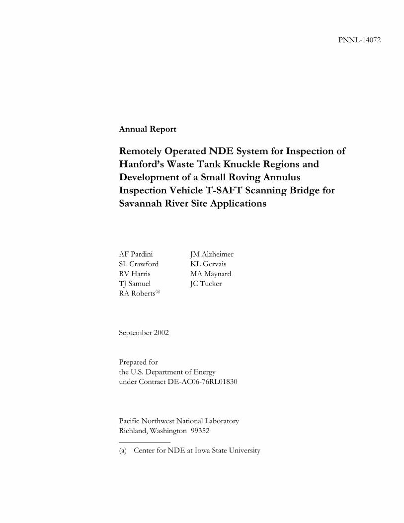
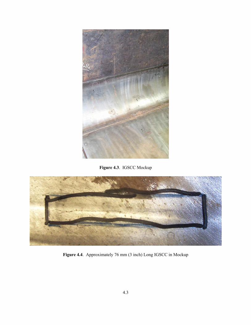
Figure 4.2. EDM Mockup 4.3 IGSCC Mockup The IGSCC Mockup was developed to test the RONDE systems capability to detect and size real stress corrosion cracks in the knuckle region. Figure 4.3 shows the mockup with a close-up view of one of the IGSCC shown in Figure 4.4. Each of the cracks in the IGSCC mockup has different depths and lengths. Figure 4.4 provides an example of one of the cracks that was detected and sized during the RONDE equipment qualification. This crack is approximately 76 mm (3 inches) in length.

4.3

Figure 4.3. IGSCC Mockup

Figure 4.4. Approximately 76 mm (3 inch) Long IGSCC in Mockup

5.1

5.0 RONDE and SRAIV Mechanical Design The RONDE mechanical design was completed and discussed in the FY 2001 annual report. The SRAIV-SAFT system consists of two primary system components: the AMS-1T motorized magnetic wheel vehicle and the SAFT/T-SAFT Bridge Scanning System. The AMS-1T vehicle is designed and built by Force Technology. The SAFT/T-SAFT Bridge is designed and built by PNNL. Figure 5.1 shows the overall system.

Figure 5.1. Small Roving Annulus Inspection Vehicle-SAFT

5.2

5.1 Magnetic Wheel Vehicle The Force Technology AMS-T1 Vehicle maneuvers the SAFT/T-SAFT bridge on the tank wall. The bridge hangs from the vehicle like a pendulum. This feature permits the vehicle to turn in any direction and transverse the wall at any angle desired. Force Technology recommended that the camera be removed from the vehicle and that the bridge be attached to the “Magnet Wheel Support Plate.” There are four M4 holes for interface mounting. Figure 5.2 shows the completed SRAIV attached to the Force Institute crawler.

Figure 5.2. SAFT/T-SAFT Bridge Attached to the Force Institute Crawler

5.3

5.2 SAFT Bridge The bridge controls the X and Y movements of the transducers. It uses high precision linear worm drive assemblies for positioning. The maximum X scan distances are 305 mm (12 inches) and the maximum Y scan distance is 152 mm (6 inches). Figure 5.3 shows the scanning bridge.

Figure 5.3. SAFT/T-SAFT Bridge The Compumotor brand stepper motors mounted on the bridge control accurate positioning of the transducers. The transducers are mounted on spring steel arms. By itself, the bridge measures 909 mm (35.8 in.) wide, 937 mm (36.9 in.) long and 99 mm (3.9 in.) high when in the collapsed state. The bridge weighs approximately 8.4 kg (18.5 pounds). The spring steel arms permit scanning on both the tank wall and the tank knuckle (see Figures 5.4 and 5.5). These transducers have the ability to be lifted from the tank wall for the journey to the scan location. Once the bridge has been positioned at the scan location, electromagnets are activated to lock the bridge in place for the scan. The electromagnets also prevent the spring steel arms from pushing the bridge away from the tank wall. The spring steel arm curvature is compressed when the arms are retracted.

5.4

Figure 5.4. The Bridge X-scan Spring Arms Capable of Scanning on the Wall and the Knuckle

Figure 5.5. X-Scan Spring Arms Placing Transducers on the Knuckle

5.5

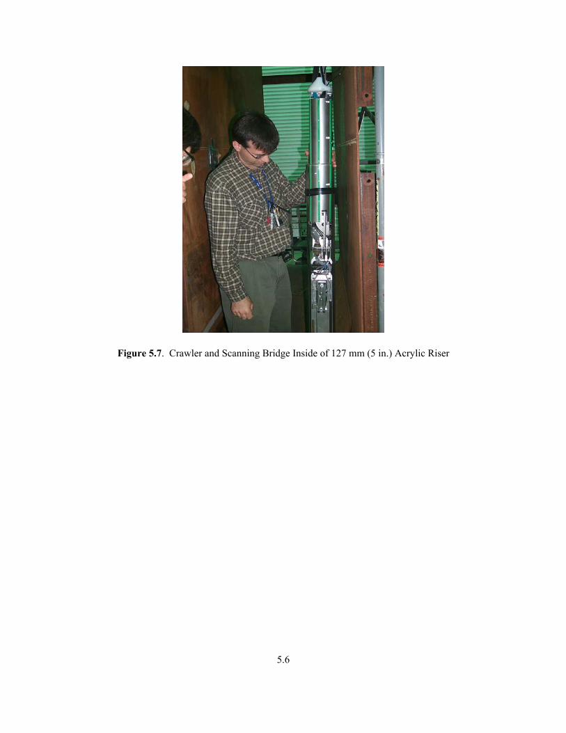
After completing the scan, the bridge magnets are released and the crawler is driven forward approximately 152 mm (6 inches) or less. The vehicle encoder ensures the accuracy of the distance driven forward. The scan process is then repeated. When scanning is completed the SAFT/T-SAFT scanning bridge is closed and the entire system is retrieved from the tank annulus. Figure 5.6 shows the SRAIV crawler and scanner in the closed position for retrieval. Figure 5.7 shows the SRAIV crawler and scanner within a simulated 127 mm (5 inch) riser.

Figure 5.6. SAFT/T-SAFT Scanning Bridge in the Closed Position

5.6

Figure 5.7. Crawler and Scanning Bridge Inside of 127 mm (5 in.) Acrylic Riser

6.1

6.0 RONDE and SRAIV Control System The RONDE control system was completed and discussed in the FY 2001 annual report. The SRAIV-SAFT control system is composed of three main components:

• SRAIV-SAFT scanning bridge • Tank top electronics • Control station

The diagram shown in Figure 6.1 provides the general layout of components at the SRS tank farm. Approximately 30 m (100 ft.) of multi-conductor cable separates the crawler/scanning assembly from the tank top electronics. A computer, pulser/receiver, and motor controls reside in the tank top electronics enclosure. Operation of the T-SAFT scanning bridge is done remotely using a fiber optic link connected to a remote computer and can be done at great distances. Crawler operation is performed by SRS using a Force Institute control station.

SRAIV Control Trailer

Ritec Pulser

Ritec Receiver

Instrument Drawer 001

Industrial PC

Data Acquisition Computer

Tank Top Instrument Enclosure

Fiber Optic Cable

100 ft. Cable

Riser

Force Crawler

PNNL SAFT Bridge

Tank Knuckle

Figure 6.1. General Layout Diagram

6.2

6.1 SRAIV-SAFT Control PNNL designed the SRAIV-SAFT control system around existing control architecture that was developed under a previous contract with the U. S. Nuclear Regulatory Commission (USNRC). Control system design is similar to the previous NRC SAFT/T-SAFT control system designs, with the main exception being that newer hardware has replaced the motor control system. In this case a Parker 6K4 universal controller has replaced a Parker AT6400 motor controller. The new 6K4 controller is self-contained, and utilizes either serial communications or Ethernet communications for the connection to the host computer. The older AT6400 controller was mounted in the host computer on the ISA bus. Since the ISA bus has been removed from most new computers, it was decided that it was time to upgrade the motor controller from previous SAFT/T-SAFT systems. For the SRAIV system, a serial link between the host computer and the 6K4 controller was used. The 6K4 controller is a low level motor controller that works in conjunction with the Parker OEM stepper motor drives. It provides an interface between the motor drives, which supply power to the stepper motors, and the host computer. Commands are given to the 6K4 controller by the host computer, which is translated into electrical pulses that are sent to the stepper motor drives. The stepper motor drives translate these electrical pulses into motor drive pulses for the stepper motors. Motor control for the RONDE system is done via several commands that are sent to the 6K4 controller. Most of these commands are identical to the AT6400 model, but some commands are either changed or removed entirely. The SAFT/T-SAFT software, running on the host computer, sends the control commands through a Parker developed driver for the 6K4 controller. A function is called within the SAFT/T-SAFT software that links with the Parker driver, in order to send the commands through the serial link. The advantage of this system is that the Parker driver allows multiple connections to it, which allows easier debugging of the software. Commands that have been sent by the driver are readily visible during debugging, as well as the response from the controller. The 6K4 controller will then send signals to the motor drives to move the stepper motors. Once the motors have been commanded to move, the software listens for motor pulses using a high-speed counter module that is used to synchronize the motor movement with data collection. This allows accurate sample timing and position information for each data set. 6.2 Tank Top Electronics The tank top electronics will be located near the entrance riser to the tank annulus. Multi-conductor cables extend from the tank top electronics enclosure to the SRAIV crawler and scanning bridge. Housed in the tank top enclosure are electronics for driving the scanning bridge mechanisms, and the ultrasonic pulser/receiver for inspection of the tank knuckle. Figure 6.2 shows the tank top enclosure and associated electronics. Section 7 of this document discusses the tank top electronics in greater detail.

6.3

Figure 6.2. SRAIV-SAFT Tank Top Enclosure 6.3 SRAIV-SAFT Control Station The SRAIV-SAFT control station provides the computing hardware necessary to perform the data acquisition and data analysis. The control station consists of a single computer that performs two functions:

• Data acquisition • Data analysis

7.1

7.0 SRAIV Electronics The electronics design was based on a previous design of a SAFT/T-SAFT system developed by the NRC as well as the RONDE system. Much of the electronics was specified as a requirement to be compatible with the old SAFT/T-SAFT software that was being implemented. Further narrowing of the electronics was specified to be the natural progression of industry standard upgrades for the existing equipment to the latest designs while still being compatible with the existing software with minimal changes. As a result the following hardware is used.

• Compumotor 6K4 RS-232 serial port controller • National Instruments 32 bit PCI slot PCI-6602 • Tektronix – Gage Compuscope 12 bit 100 Mega sample per second digitizer - PCI (dual slot) • Ritec ultrasonic square wave pulser SP-801 • Ritec broadband receiver BR-640

PNNL is currently using a Parker OEM drive to control the stepper motors on the SRAIV scanning bridge. During the enhancement work this year on the RONDE system, a low noise stepper motor driver was found which virtually eliminated noise in the system. Built by Precision Motion Controls, these motor drives would enhance the current SRAIV system. PNNL recommends that as an enhancement to the SRAIV prototype, new low noise stepper motor drives replace the current Parker OEM drives. The LinEngineer stepper motor was chosen for the X1 and X2 drives on the scanning bridge because they are smaller size, weight, and bolt pattern and fit within the tight constraints given. The computer that resides in the tank top enclosure has been upgraded to an industrial grade 2.5 GHz Pentium computer running Windows XP operating system. Cyber Research specializes in thin line rack mount computer systems.

8.1

8.0 RONDE Enhancements 8.1 Improving the Ultrasonic Signals The data acquisition system includes the PC platform, analog to digital (A/D) conversion electronics, pulser-receiver electronics, signal conditioning electronics and filters, and the front-end scanner-transducer-coupling system. Any field-ready and reliable inspection system must be built upon a robust structural framework for data acquisition. Of primary importance to the entire system is the PC platform on which the inspection system resides. PNNL has upgraded the RONDE system to the fastest available PC platform commercially available. The tank-top computer is now a 2.5 GHz machine operating with Windows XP. The Control station computer is a dual Zeon processor 2.2 GHz machine optimized for data analysis. In order to enhance the dynamic range capability of the ultrasonic signals, a high-speed, 12-bit A/D converter with expanded memory capability was implemented. This significantly improved the system’s data acquisition speed and dynamic range, and provided a more efficient method for invoking linear waveform averaging in order to reduce random and electronic white noise introduced by amplifiers and other environmental sources. PNNL implemented numerous hardware noise suppression techniques to overcome the various noise sources inherent in the prototype RONDE system. The largest contributors to the noise problem were the stepper motor drivers that were used. Previous experience in other PNNL systems indicated that stepper motor drives that pulse width modulated the motor input produced a large amount of noise on the ultrasonic signal. When the system was under development, PNNL contacted Parker (supplier of Compumotor motors and drives) and purchased their lowest noise motor and drives. These were acceptable (i.e., signal to noise ratio was acceptable based on signal averaging) at the time, but PNNL continued to pursue a less noisy set of electronics. Further investigation found that a supplier (Precision Motion Control) provides a low noise motor driver that does not pulse width modulate the input. PNNL recently replaced the stepper motor drives, which greatly improved the signal, thereby allowing data acquisition with no averaging. In the past the motor noise was overcome by an averaging algorithm, however this prevented the system from operating at an optimum speed. Previous scanning speeds ranged from 5.1 to 7.6 mm (0.2 to 0.3 inches) per second in the “X” direction (vertical movement of the transducer), which translated to approximately 32 minutes to scan a 305 mm (1-ft) length around the tank. With the new improvements scan speed is now 38 mm (1.5 inches) per second which translates to approximately 11 minutes to scan a 305 mm (1-ft) length around the tank. To make enhancements to the system such as changing the motor drivers, etc. also require changes in software and other data acquisition hardware. A complete list of changes that were done to improve the ultrasonic signal and data acquisition speed follows:

• New Motor Drives (LN-2 from Precision Motion Control)

• New 6K4 Motor Controller (Previous motor controller required an ISA slot and the newer faster computers no longer support the ISA bus. The replacement 6K4 board fits into a PCI slot.)

8.2

• New PCI 6602 Counter Timer (Utilizing the off the shelf counter timer card and National Instruments breakout box allows for upgrading to faster computer (previous counter timer card was ISA), requires less circuitry, and allows computer control of remote electromagnets on the RONDE scanning bridge.)

• New tank-top computer (Upgrading the tank-top computer allowed PNNL to use the new 6K4

controller and counter timer card, and increased the stability of the system operating with Windows XP. Utilizing Windows XP and it inherent remote operation capability, allows PNNL to remotely monitor the entire A-Scan display in real time, which was impossible using the older technology.

• Upgrade to Gage Compuscope 12100 (12-bit) Digitizer (To extend the detection capability it was

necessary to improve the dynamic range and resolution of the system. This enhancement changed the system configuration from an 8-bit system to a 12-bit system providing considerably more dynamic range).

• Implemented Noise Suppression Techniques (Additional noise suppression was implemented, such as

additional shielding of coaxial cables). 8.2 Enhancements to Improve User Friendliness 8.2.1 Provide Operator with new Software Capabilities and Controls Many of the enhancements to improve the user friendliness of the system were software related. The initial system was very cumbersome in operation since many of the operations were done manually or required numerous steps and hand calculations. For instance, PNNL has added the automatic “Home” and “Park” capability to the RONDE scanning system. With a simple keystroke the transducers can be positioned to the “Park” position (transducers are moved to a position off of the tank surface and the scanning bridge is positioned in the middle of the scanning range). This “Park” position allows for movement of the scanning bridge without damaging transducers and places the transducers in a balanced “Y” position so that the scanning bridge may be aligned to the upper knuckle weld. When it is time to perform a scan, the “Home” position moves the transducers to a start position and aligns the two transducers to begin a scan sequence. Another software improvement was the “Get” function, which provides a digital readout of where the transducers are located on the scanning bridge (in X1, X2, and Y positions). Additional software was written to correlate position of the transducer with the crawler encoder position. In an effort to assist the operator during the Y translation of the crawler, a tilt sensor was added to the system and a software function was included to provide a digital readout of this tilt position. Other software modifications are listed below:

• Changing the T-SAFT code to operate under the Windows XP operating system.

• Modifying the T-SAFT code to implement the new 12-bit digitizer card.

8.3

• Modified the data acquisition software for the increased scanning speed, which was possible with the

reduced noise motor drives.

• Disabled software features of the laboratory T-SAFT code which are not applicable to this inspection. This restricts the operator’s software input and provides less confusion.

8.2.2 Streamline the Ultrasonic Detection and Analysis Procedure Up until recently the ultrasonic procedure utilized pulse echo (PE, sending and receiving the ultrasonic pulse from the same transducer) for flaw detection. The procedure sequence began with a PE scan to detect the upper knuckle weld, which could be used as a fiducial mark in setting up the scanning. With the weld located in the “X” coordinate, a PE scan was then completed for flaw detection over the entire 1-ft. length (circumferentially around tank). If a flaw was detected and located, a new pitch-catch (PC, sending the ultrasonic signal from one transducer and receiving with another) scan was implemented to select the plane of the flaw for tandem sizing setup. Once the plane of the flaw was determined, tandem sizing was performed. Because the PC method requires more gain in the system than PE, it was not advisable to perform detection since the noise became excessive. With the advent of the many changes described in section 2 above, PNNL was able to perform the detection scans with PC thereby eliminating the need to perform PE. The cascade effect allowed for removal of noise inducing components such as the pre-amplifier, diplexer, and the remote switching necessary to change from PE to PC. All of these changes streamlined the procedure considerably and allows the operator to simply perform a detection scan and directly perform a tandem sizing without any change to the ultrasonic system. An additional electronic component was designed and fabricated to provide an easier method for the operator to perform distance amplitude correction of the ultrasonic attenuation. PNNL designed and fabricated a time variable gain amplifier (TVGA). The TVGA provides a uniform amplitude of the flaw signals based on distance (time) from the transducer. The TVGA improved detection capability at extended distances from the transducer. 8.3 Mechanical Enhancements The prototype RONDE system underwent a few mechanical modifications to improve operability and stability. Modifications included installing dust and rust covers over key rotating components and installing limit devices on all axes. These limit devices included travel limits and transducer stops. To provide more robust scanning, the motors driving the two “X” axes were rotated 90 degrees to provide a direct drive. Deployment of the RONDE system is more complex than the P-Scan crawler currently used on the Hanford tanks. PNNL designed and fabricated a deployment platform that allows the RONDE system to be deployed in the annulus in a safe configuration. Figure 8.1 shows the new deployment platform with the RONDE system position for deployment.

8.4

Figure 8.1. RONDE Deployment Platform 8.4 Flaw Detection and Characterization Evaluation 8.4.1 Extended Distance Evaluation A significant feature of the RONDE system is its ability to detect flaws beyond the knuckle region and under the waste tank. Many of the enhancements mentioned previously made detection and visualization of the flaws possible. Prior to this years work the RONDE system was unable to display much past the knuckle region itself. Figure 8.2 shows the imaging capability possible by the end of FY01. Notice that no time variable gain was implemented. In evaluating the figure, the pink band on the left is the upper knuckle weld and the signal is extremely saturated. On the right is a red and green band, which is the lower knuckle weld. In between are two EDM notches that are both 20% through-wall. Implementing the TVGA allows to display this two 20% flaws at the same amplitude. Also notice that the welds look approximately the same. PNNL designed and fabricated the time variable gain amplifier for the distance amplitude correction necessary to account for attenuation over the long metal paths. Figure 8.3 shows the current RONDE imaging capability, all based on the enhancements mentioned previously. Figure 8.4 provides an image of the entire distance from the upper knuckle weld to the end of plate signal, approximately 6-ft. from the transducers.

8.5

Figure 8.2. Imaging Capability at the End of FY01

Figure 8.3. Imaging the Knuckle with the Current RONDE System

8.6

Figure 8.4. Imaging the Entire Knuckle and Beyond 8.5 Axial Crack Evaluation PNNL evaluated the axial crack detection capability of the RONDE system. Initial measurements were made on flat plate looking at sawcuts. Sawcuts are mirror type reflectors, and skewing the 70-degree shear wave transducer a couple of degrees decreased the signal to zero. However, the morphology of an IGSCC is considerably different. Hand measurements indicated that an IGSCC could be detected with a skew of up to approximately 30 degrees.

8.6 Pitting Evaluation Detection of pits in the knuckle region is very difficult if not impossible with the technique used on the RONDE system. Normal inspection for pits includes a zero degree pitch/catch arrangement transducer located directly over the pit. Even in this configuration it is difficult to ascertain whether the anomaly is a pit or some other form of localized corrosion. Performance testing utilized to qualify the existing P-Scan system for examination of the Hanford waste tanks include smooth hemispherical pits of different diameters

Upper Knuckle Weld

Lower KnuckleWeld

TransitionWeld

End of Mockup

All 20% EDM Notches (1”L x 0.025”W x 0.22”D

19” 36” 12”4”

8.7

and depths. Figure 8.5 illustrates the difficulty when trying to detect a pit using an angle beam transducer (or a straight beam transducer for that matter). The amount of energy returned to the transducer from the face (curve) of the pit is very small because of the reflection angle from the curved surface. PNNL evaluated pits of various depths and diameters in three locations around the tank knuckle.

Transducer Transducer Transducer

Figure 8.5. Energy Direction Returned from Hemispherical Reflector Figure 8.6 shows the final stages of the pits that were installed in the mockup for evaluation. Pits were machined into the mockup and then it was scanned and evaluated. The same pits were then deepened (trying to maintain a 3 to 1 diameter to depth ratio) and rescanned for evaluation. This sequence was repeated and Table 8.1 summarizes the results. None of the pits in the table were detected using the RONDE system prior to the enhancements.

Figure 8.6. Array of Machined Pits

A

B

C

8.8

Table 8.1. Pit Analysis

Location A Target Pit Depth

(inches) Measured Pit Depth

(inches) Measured Pit Diameter

(inches) Detected 0.045 0.049 0.109 N 0.090 0.095 0.247 N 0.135 0.134 0.450 N 0.180

0.219 (25% Throughwall) Location B

Target Pit Depth (inches)

Measured Pit Depth (inches)

Measured Pit Diameter (inches)

0.045 0.045 0.110 N 0.090 0.091 0.240 N 0.135 0.134 0.44 N 0.180 0.178 0.495 N

0.219 (25% Throughwall) 0.223 0.65 N Location C

Target Pit Depth (inches)

Measured Pit Depth (inches)

Measured Pit Diameter (inches)

0.045 0.044 0.112 N 0.090 0.105 0.247 N 0.135 0.136 0.397 N 0.180 0.183 0.542 N

0.219 (25% Throughwall) After the enhancements listed in Sections 8.2 and 8.3 above were implemented the detection of pits was only slightly improved. This improvement was probably more aligned with corrosion products beginning to build in the pit area providing larger energy return than actually higher resolution from the system. The peak response from a corroded pit was measured at –24 dB relative to a 20% through-wall notch, while the noise level was –30 dB. This gives a signal to noise ration of two to one (6 dB). For comparison, an IGSCC response was –10 dB. Therefore, even though the pits were imaged, their responses are significantly below the detection threshold. This agrees with the modeling discussed in section 10 of this document. No further pitting evaluations were performed. 8.7 Wall Thinning Evaluation Wall thinning measurements could only be made if PNNL was able to image the inside and outside surfaces of the knuckle plate. To do this, PNNL would have to provide a system that was capable of

8.9

imaging surface anomalies such as scratches and surface finishes. The resolution of the current system is not capable of performing at this level, so no further investigation was done. 8.8 Future Improvements to the RONDE System The design of the RONDE system was driven by cost and schedule. Building the prototype system was based on using existing software and modifying it as necessary to perform the data acquisition. The design allowed for implementing the T-SAFT technology in multiple configurations. For example, scanning currently takes place above the upper knuckle weld. This allows for examination of the knuckle and beyond without having to be in proximity to it. In the case of some Savannah River Site (SRS) tanks, an exhaust pipe lies on the floor of the annulus making it difficult to scan on the knuckle. This design accommodates this configuration. The technology can be changed or modified to improve both detection and characterization. Moving the transducers below the upper knuckle weld will only improve signal quality and extend the reach of the detection and characterization capability. It also improves the chances of performing pitting evaluations and wall thinning. In FY02 PNNL designed and fabricated a scanning bridge for application to SRS waste tanks. In Figure 8.7, the dual spring- steel scanning mechanism could be adapted to the Force Institute P-Scan system used at Hanford to provide a reliable method of scanning the knuckle with T-SAFT below the upper knuckle weld and improving detection and characterization capabilities.

Figure 8.7. SRS Spring Steel Scanning Arms Other possible improvements include:

• Modifying the SAFT analysis code to allow for selecting the region on the display that needs processing, and only processing that region. The current system requires you process the entire data set, which takes considerably more time.

8.10

• Improve data visualization tools. Being able to display the data in 3 dimensions would be a great asset in understanding the flaw characteristics.

• Directly correlate the mathematical modeling performed by Iowa State University with the SAFT

algorithms to better predict the plane of the flaw for sizing and assist in the decision whether the flaw is an inside diameter (ID) or outside diameter (OD) flaw.

9.1

9.0 FY02 Test Results 9.1 Flaw Detection The RONDE system is operated in the pitch-catch mode for defect detection. PNNL performed numerous tests to verify detection capability of the RONDE system. All flaws in all of the mockups that were greater than the depth specified in the functions and requirements were reliably detected. This included all of the IGSCC in the new mockup. Figures 9.1, 9.2, and 9.3 show a C-scan images of each IGSCC in the knuckle mockup. In Figure 9.1, the solid band on the left of the image is the upper knuckle weld and the solid band (partly occluded by the deep crack) on the right is the lower knuckle weld. Crack #2 is a deep long crack approximately 178 mm (7 in.) in length. Figures 9.2 and 9.3 demonstrate the RONDE’s imaging capability in the detection, location, and length sizing of IGSCC in the knuckle mockup.

Crack #1

Crack #2

Figure 9.1. C-Scan Image of IGSCC in the Knuckle of Mockup

9.2

Figure 9.2. IGSCC #3 in the Knuckle Mockup

Figure 9.3. IGSCC #4 in the Knuckle Mockup

9.3

As discussed in Section 8 of this report, enhancements were done to extend the reach capabilities of the imaging system to detect flaws beyond the knuckle region. Figure 9.4 provides an image of the RONDE systems capability to detect IGSCC beyond the knuckle and under the waste tank. In Figure 9.4, the enlarged image clearly shows the IGSCC beyond the lower knuckle weld.

Figure 9.4. IGSCC Detected in Mockup Beyond Lower Knuckle Weld 9.2 Flaw Sizing Tandem SAFT or T-SAFT provides a means for sizing the depth or through-wall dimension of vertically oriented planar defects. A transmitting and receiving transducer are simultaneously scanned, in tandem, in the region of interest. The peak response from the corner trap of a flaw is first located with pitch-catch ultrasonic data as shown in Figure 9.5. For tandem data acquisition the two tandem transducers are positioned side by side at this peak response location. This location will produce a peak response in both the tandem and pitch-catch data. The transmit and receive transducers are moved 76 to 102 mm (3 to 4 in.) in opposite directions. The tandem data acquisition then begins by scanning the two transducers towards each other, up to the mid-point of the scan, and continuing away from each other, to the end of the scan line as shown in Figure 9.6. Next the pair of transducers returns to their start positions, are both incremented circumferentially, and start the next scan line. In this way tandem data can provide length as well as depth information.

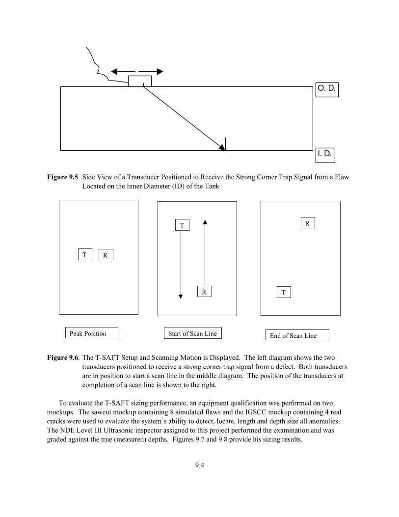
9.4

I. D.

O. D.

Figure 9.5. Side View of a Transducer Positioned to Receive the Strong Corner Trap Signal from a Flaw

Located on the Inner Diameter (ID) of the Tank

T R

T

R T

R

Peak Position Start of Scan Line End of Scan Line

Figure 9.6. The T-SAFT Setup and Scanning Motion is Displayed. The left diagram shows the two

transducers positioned to receive a strong corner trap signal from a defect. Both transducers are in position to start a scan line in the middle diagram. The position of the transducers at completion of a scan line is shown to the right.

To evaluate the T-SAFT sizing performance, an equipment qualification was performed on two mockups. The sawcut mockup containing 8 simulated flaws and the IGSCC mockup containing 4 real cracks were used to evaluate the system’s ability to detect, locate, length and depth size all anomalies. The NDE Level III Ultrasonic inspector assigned to this project performed the examination and was graded against the true (measured) depths. Figures 9.7 and 9.8 provide his sizing results.

9.5

Wes Nelson Sawcuts

0

0.2

0.4

0.6

0 0.5 1

UT Measured DataTr

ue S

tate

Dat

a

PerfectPerformance

UT MeasuredData

Figure 9.7. Sizing Results on Machined Sawcuts

Wes Nelson Cracks

00.20.40.60.8

0 0.2 0.4 0.6 0.8

UT Measured Data

Truc

e St

ate

Dat

a

UT MeasuredDataPerfectPerformance

Figure 9.8. Sizing Results on IGSCC 9.2.1 Machined Defects Sizing The accuracy requirement for depth sizing of machined defects is a root mean square (RMS) value of 2.54 mm (0.1 in.). Figure 9.7 is a plot of the data provided by NDE Level III Ultrasonic inspector Mr. Wes Nelson. Mr. Nelson’s RMS value for all machined defects is 1.4 mm (0.055 in.), well below the 2.54 mm (0.1 in.) criteria. 9.2.2 Inter-Granular Stress Corrosion Cracks (IGSCC) The requirement for sizing IGSCC is the same as the requirement for the machined defects, namely 2.54 mm (0.1 in.). Figure 9.8 is the plot of the data provided by Mr. Nelson. The RMS value of this data is 1.8 mm (0.07 in.), which is well within the 2.54 mm (0.1 in.) requirements.

10.1

10.0 Computer Modeling of the Knuckle Region 10.1 Computer Model Studies at CNDE (Iowa State University) This section describes the development and application of a computer model designed at the Center for Nondestructive Examination (CNDE) at Iowa State University to aid in the design and data interpretation of the T-SAFT inspection. Work in the previous year focused on the development of this computer model. The work performed this year applies the model to the study of T-SAFT performance issues. Work this year examined the relative sensitivity of the inspection in detecting pit-like defects, as opposed to crack-like defects. This examination entailed the extension of the computer code to handle the more complicated ray geometry involved in reflection from a spherical pit, summarized below. Work this year also addressed the understanding and more efficient use of the information contained in the complicated “wave packet” signals obtained in the T-SAFT measurement. Considering first the planar shell geometry, it is shown that a single wave packet contains information equivalent to several T-SAFT measurement positions. Effective use of this information could significantly reduce the required amount of T-SAFT data collection. Indeed, it is shown that a single wave packet can contain enough information to perform a complete flaw sizing analysis. These results motivate future work to extend this analysis to the significantly more complicated case of the curved shell. 10.1.1 Scattering by Spherical Pit A summary of the model developed last year is first presented. The radiation by the transducer/wedge assembly is modeled by a point source located on the surface of the steel shell with an angular-dependent radiation pattern, as shown in Figure 10.1. The angular dependence is specified as follows. Considering first radiation by the transducer into the plastic wedge material, the radiation pattern is assumed to consist of a single lobe that has an angular dependence represented by a squared cosine function. Rays emanating from this single lobe are transmitted into the steel with transmission angles determined by Snell’s law, and with amplitudes determined by the corresponding plane wave transmission coefficient. The single parameter controlling this radiation pattern is determined either by calibration experiments, or by assuming the transducer performs as a perfect piston radiator. The measurement uses a 3.5 MHz, 12.7 mm (0.5-inch) diameter transducer mounted on a wedge designed for 70-degree shear wave transmission. Calibration measurements determined that the transducer has a 7.5 degree 6-db angular bandwidth when radiating into steel. The rays radiated by this point source are transmitted to the location of the flaw using ray theory. Figure 10.2 shows transmitted ray geometries for a 24 mm (15/16-inch) thick shell having a 305 mm (12 inch) radius, for three different angles of angles transmission θ1. The ray theory applied to the problem computes both ray geometry and field amplitudes along the rays, using appropriate extensions of fundamental ray theory to account for focusing phenomena associated with multiple reflections off the concave outer shell wall. The principals underlying this aspect of the model are presented in detail in last year’s annual report (Pardini et al. 2001; Roberts et al. 2001). The rays plotted in Figure 10.2 lie in the

10.2

θ1

(a)

‘in-plane’ ray ‘out-of-plane’ rays

2

transducer symmetry plane

(b)

Figure 10.1. Geometry of Radiation by the Transducer/Wedge Assembly into Steel

measurement symmetry plane, defined by θ2 = 0 in Figure 10.1b. The geometry of rays propagating outside of the measurement symmetry plane is easily determined from the in-plane ray geometry, under an assumption that out-of-plane shell curvature can be ignored. The signal generated by the flaw is computed using Auld’s reciprocity relation applied over the flaw surface (Auld 1979). This relation states that the transducer output voltage in response to a flaw can be determined by integrating the product of the field on the flaw surface, and the field that would exist in the absence of the flaw (the incident field), over the flaw surface. In last years work, the flaw was assumed to be a planar crack oriented perpendicular to both the shell surface, and the direction of beam propagation. Again, the details of the computation of crack signals using Auld’s reciprocity relation is presented in detail in last year’s report.

10.3

transducer transducer

transducer

flaw plane flaw plane

flaw plane

(a)

(c)

(b)

Figure 10.2. Ray Geometry for Rays Emerging from the Transducer at Angles of (a) 60 Degrees,

(b) 70 Degrees, and (c) 80 Degrees Work this year extended the flaw scattering formalism to consider scattering by a spherical pit, rather than a planar crack. This extension builds upon the existing model as follows. A key computation in the calculation of the crack signal is to determine the location and direction at which the transmitted rays cross the plane containing the crack. The distance s of the intersection point from the inner shell wall, and the direction of propagation φ at the intersection point, as shown in Figure 10.3, are tabulated as a function of transmission angle θ1, along with the corresponding field amplitude and phase at that position. For example, a plot showing the distance s as a function of ray transmission angle is presented in Figure 10.4, corresponding to the ray transmission depicted in Figure 10.3. The algorithm for scattering by a spherical pit uses this tabulated data as input to determine the wave field on the pit surface.

10.4

Transmitted Ray

crack plane sInner shell wall

φ

Figure 10.3. Geometry of Ray Intersecting the Reference Plane Containing the Crack

S

θ Figure 10.4. Position of Ray Intersection s on the Flaw Reference Plane as a Function of Ray

Transmission Angle θ The spherical pit is oriented in relation to the flaw plane, hereafter referred to as the “reference plane,” as shown in Figure 10.5. Within the plane of the shell wall, the mouth of the pit is tangent to the reference plane. The pit has a radius R, and a depth h. The wave field on the pit surface is evaluated by extending rays from positions on the reference plane to the intersection point on the pit, if an intersection exists. The ray intersection with the pit surface is designated by the angle ν, as shown in Figure 10.5. The pit intersection angles are thereby tabulated as a function of ray transmission angle θ1, as are the increments in propagation distance L. It is assumed that the change in the field amplitude occurring over the increment L is negligible, hence the field amplitude on the pit surface is assumed equivalent to that

10.5

evaluated on the reference plane. To perform the surface integration called for in Auld’s reciprocity relation, the tabulated wave field on the pit surface is inverse-mapped onto pit intersection angle ν. The surface integration is then performed with ν as the integration variable. The inverse mapping entails a rather complicated algorithm, due to the fact the mapping is not one-to-one: multiple rays can intersect a given point on the pit surface. This point will be illustrated in the numerical examples presented below.

Figure 10.5. Orientation of Spherical Surface Pit in Relation to the Reference Plane The calculation described in the previous paragraph is straightforward when considering rays propagating in the measurement symmetry plane (θ2 = 0 in Figure 10.1b). Additional complications are encountered when considering out-of-plane ray propagation, as depicted in Figure 10.6a. To simplify the treatment of the out-of-plane ray intersection, a mild assumption is imposed stating that the rays emanating from the reference plane are all propagating parallel to the measurement symmetry plane. This condition is depicted in Figure 10.6b. This assumption is equivalent to stating that wave fronts are approximately linear in the out-of-plane direction over the extent of the flaw. This is a robustly valid assumption for the transducer-to-flaw distances encountered in the inspection. The surface of the pit is parameterized in cylindrical coordinates ν, z, where ν is the pit intersection angle as previously depicted, and the z axis intersects the center of the sphere defining the pit, running parallel to the shell surface and reference plane. The surface integration is carried out using ν, z as the integration variables. Imposing that rays emanating from the reference plane are all parallel significantly simplifies the inverse-mapping of the wave field from the transmission angle coordinates to the surface integration coordinates, since rays transmitted at a fixed out-of-plane angle all intersect the pit at the same value of z, resulting in a one-dimensional rather than two-dimensional interpolation in performing the inverse-mapping. An additional complexity encountered when treating out-of-plane ray intersection is depicted in Figure 10.7. Figure 10.7 plots ray geometry in the plane parallel to the measurement symmetry plane but displaced by the distance z, as indicated in Figure 10.6b. It is noted that, in this cross-sectional plane, the pit profile does not touch the reference plane, that is, there is a segment of shell surface lying between the reference plane and the pit. The ray geometry in Figure 10.7 depicts the case of a ray emanating from the reference plane that reflects from the shell wall prior to intersecting the pit surface. The algorithm for determining the wave field on the pit surface identifies and treats these cases.

10.6

In-plane ray

Out-of-plane ray Pit intersection

Reference plane

(a)

Reference plane

Out-of-plane ray

Parallel ray segment

True intersection

Approximate intersection

z

Symmetry plane

(b)

Figure 10.6. Top View of Ray Geometry at the Spherical Pit: (a) “Out-of-Plane” Ray Intersection on

the Spherical Pit, (b) Parallel Ray Approximation Used in Field Evaluation on Pit Surface

10.7

Reference plane

Shell wall reflection

Pit surface intersection

Figure 10.7. Possible Additional Surface Reflection for Out-of-Plane Transmitted Rays Numerical results are now presented demonstrating the model function, and comparing the relative strength of signals generated by cracks versus spherical pits. The shell geometry, transducer location, and flaw location correspond to those depicted in Figure 10.3. A single transducer used in pulse-echo mode is assumed. The transducer is positioned on the outer shell wall 25.4 mm (1 inch) from the wall-knuckle transition. The flaw is located at the knuckle-bottom transition, extending into the shell from the inner shell wall. Results are compared first for a crack and pit that extend 80 percent through the shell wall thickness. The pit has a radius equal to 90 percent of the shell thickness, implying that it is not quite hemispherical. The crack is assumed to have a shape profile equivalent to the central cross-section of the pit, that is, a section of a circle having a radius 90 percent of the shell thickness, and a crack depth of 80 percent of the shell thickness. The in-plane ray intersection position on the reference plane (the plane containing the crack) as a function of transmission angle θ1 was previously shown in Figure 10.4. Note in this plot that the crack extends over the bottom 80 percent of the vertical scale. It is seen that as many as 11 ray intersection occur on the crack face. It is these numerous ray intersections that give rise to the numerous signal components observed in the recorded wave packets, as discussed in detail in last years report. The corresponding pit intersection angle ν is plotted as a function of transmission angle in Figure 10.8. The gaps in the plot in Figure 10.8 correspond to angles of transmission for which rays do not intersect the pit surface. Again it is seen that numerous rays intersect given points on the pit surface, giving rise to the multiple reflected signal components comprising the wave packet. The signals generated by reflection from both the crack and pit are computed through evaluation of Auld’s reciprocity relation over the flaw surface. Auld’s reciprocity relation considers time-harmonic wave fields, hence the signal is first computed frequency-by-frequency over the bandwidth of the transducer. The computation assumes the spectral response of the transducer is adequately represented by a squared cosine function. A 70 percent 6 dB spectral bandwidth was specified, determined by experimental calibration measurements. Time domain signals are then obtained through Fourier transformation of the spectral data. The time domain responses to the 80 percent through-wall crack and pit are compared in Figure 10.9. It is noted that the peak signal amplitude from the crack is 26 times larger than that of the pit, or a 28 dB difference. This difference in signal strength is consistent with experimental observations of signals from a crack verses a spherical pit.

10.8

θ1

ν

Figure 10.8. Pit Intersection Angle as a Function of Ray Transmission Angle for an 80 Percent Through-Wall Pit

Results are next compared for a crack and pit that extend 20 percent through the shell wall thickness, located on the inner shell wall. The radius of the pit is assumed to be 25 percent of the shell thickness. Again, the crack is assumed to have a shape profile equal to the central cross-section of the pit. The transducer and flaw positions are the same as for Figure 10.9. Plots comparing the signals received from the crack and pit are displayed in Figure 10.10. It is seen in this case that the crack signal is 18 times larger than the pit signal, or a 25 dB difference. 10.1.2 Wave Packet Analysis The flaw signals received in the tank shell inspection are in the form of wave packets comprised of numerous discrete signals, as observed in Figures 10.9 and 10.10. Last year’s work focused on explaining the origin of the components in these wave packets. Detailed analysis of the propagation phenomena underlying the wave packet structure can be found in last year’s final report. The T-SAFT data processing currently applied to the wave packets is based on the assumption of a single propagation path from the transducer to the flaw, and data processing proceeds by identifying the largest signal in the

10.9

(a)

(b)

Figure 10.9. Comparison of Signals from an 80 Percent Through-Wall (a) Crack and (b) Pit. Note

difference in amplitude scales.

10.10

(a)

(b)

Figure 10.10. Comparison of Signals from a 20 Percent Through-Wall (a) Crack and (b) Pit. Note

difference in amplitude scales.

10.11

wave packet, and apply data processing to this component alone. It seemed plausible that the wave packet contains much more information than was being extracted from it, so a task was undertaken this year to examine this issue. The fundamental question asked by this task is: “Does the wave packet contain information that could reduce the amount of data collection required to perform flaw sizing?” The findings of this task are now summarized. The mechanism underlying the T-SAFT flaw sizing algorithm is the sweeping of a focused beam over the extent of the flaw, thereby measuring the flaw dimension by monitoring the amplitude of the reflected signal. The challenge to overcome in practical implementation is to obtain a sufficiently focused beam to resolve the flaw dimensions. As implied in the name, the T-SAFT measurement obtains this focus through synthesizing a focusing aperture by appropriately combining signals obtained from non-focused transducers at discreet measurement positions. As a rule of thumb, the sharpness of the focus is determined by the angular width of the synthesized aperture. The tandem configuration of the T-SAFT measurement is designed to improve the performance and efficiency of the aperture synthesis by collecting data at positions of maximum signal amplitude. Specifically, when imaging large planar cracks, the reflected energy by-and-large propagates in the direction of specular reflection, as specified by Snell’s law of reflection. Assuming a planar flaw with a specified orientation, the T-SAFT measurement positions the receiver to intercept the specular reflection for a given transmitter location. This is summarized in the diagram of Figure 10.11. The T-SAFT method was developed for sizing of vertical planar cracks extending inward from the far wall on a planar plate-like specimen. The measurement uses the reflection off the far wall to receive the specularly reflected signal. Signals are obtained at transmitter and receiver positions symmetrically placed about the position A noted in Figure 10.11. Position A corresponds to the position of maximum pulse-echo reflection, occurring when the direction of maximum amplitude in the transducer angular radiation pattern coincides with the ray connecting the transducer to the root of the crack. Position B identifies a second measurement position, where the transmitter and

Figure 10.11. Configuration of T-SAFT Measurement as Originally Conceived

10.12

receiver are displaced equal distances in opposite directions from position A. By collecting data over a sufficient range of transducer translation, and with sufficient position density, the signals can be phased and combined to form a response equivalent that of a highly focused transducer. The focal position of this synthetic focused beam can be swept over the plane of the flaw by controlling the phasing of the contributing signals, and the extent of the flaw determined. The effectiveness of the T-SAFT flaw sizing has been well documented in previous reports and publications. It is noted that the measurement configuration shown in Figure 10.11 is equivalent to having two transmitting and receiving transducers, one and top and one on the bottom, of a specimen having twice the thickness, as shown in Figure 10.12. The transducers behave as if they are electronically tied together, that is both transmitters fire at the same time, and the outputs of the two receivers are summed. The transducers located on the bottom surface in Figure 10.12 are referred to as virtual transducers. The concept of virtual transducers will be referred to extensively in what follows.

Virtual transducers

Figure 10.12. Equivalent Configuration to the Measurement Shown in Figure 10.11, Employing Virtual

Transducers In applying the T-SAFT measurement to long-range inspections in shells, a procedure corresponding to that described in Figure 10.11 is followed. The position of maximum pulse-echo response in identified, and used as the center point in the T-SAFT data collection. This is shown pictorially in Figure 10.13. The transducer shown is positioned 3.5V away from the root of the crack. Position A in this case corresponds the 3.5V ray path that coincides with the direction of maximum amplitude in the transducer angular radiation pattern. T-SAFT data is collected and processed in this configuration by viewing the transmitting and receiving transducers as sitting on a specimen that is 5 times the thickness of the plate specimen, depicted in Figure 10.13 as the virtual transducer positions. Data processing then proceeds identically to that applied in Figure 10.11.

10.13

Figure 10.13. Conceptual Application of T-SAFT to Long-Range Inspection of a Plate A problem encountered in viewing the long-range measurement as equivalent to the virtual measurement in Figure 10.13 is that it ignores all the other possible ray paths that connect the transducer to the root of the flaw. For example, ray paths of 0.5 V, 1.5V, and 2.5V can also be drawn, as can 4.5V, 5.5V, and so on. In the configuration shown in Figure 10.11, in which position A corresponds to 0.5V ray path, the higher-order V ray paths connecting the transducer to the flaw root occur at transmission angles for which the radiation pattern has a negligible amplitude. In contrast, in the longer-range measurement as depicted in Figure 10.13, these other ray paths can have appreciable amplitudes, resulting in the multiple signal components contained in the wave packets. The problem presented by the presence of these other signal components is a minor one: care is required in selecting the maximum component, and in properly gating that component as the T-SAFT data is processed. The notion motivating this study is the observation that the other signal components in the wave packet come from transmission and reception of rays over the entire angular radiation pattern of the transducer, implying that there is conceivably a wealth of angular spectral information contained in these signals that could be used in synthesizing a focused beam response. Effective use of this information entails developing a view of the problem that will facilitate conception of an appropriate processing algorithm. To this end, the concept of the virtual transducer, indicated in Figure 10.12, is more fully developed. Consider a beam generated by a source reflecting from a half-space, as shown in Figure 10.14a. The reflected beam in the upper half space can be viewed as originating from a virtual source in the lower half-space, as noted in Figure 10.14b. Next consider the reflection from a second planar surface, defining the upper wall of a planar plate specimen, as depicted in Figure 10.14c. The beam reflected from the upper half space can be viewed as originating from a virtual source positioned twice the plate thickness above the original (or actual) transducer, as depicted in Figure 10.14d. Thus the actual source plus first two reflections can be viewed as a virtual array of three transducers. As there are an infinite number of multiple reflections in the plate specimen, there are correspondingly an infinite number of virtual transducer positions, forming an infinite virtual transducer array, with transducers spaced a distance of twice the plate thickness. This virtual array is depicted in Figure 10.15. The wave field in the plate can be viewed as equivalent to the wave field that would exist in an unbounded medium arising from this

10.14

(a)

Virtual transducer (b)

Virtual transducer (c)

Virtual transducer

Virtual transducer

(d)

Figure 10.14. Virtual Transducer Concept: (a) Transducer in Half-Space, (b) Corresponding Virtual

Transducer, (c) Transducer on Plate, (d) Corresponding Virtual Transducers for First Two Reflections

10.15

flaw

Figure 10.15. Virtual Transducer Array in a Whole Space Containing a Flaw, Equivalent to a Single Transducer on a Plate

infinite array of transducers, all firing at once. It then follows that the signal received from a flaw in the plate will be equivalent to the response of the same flaw positioned in an unbounded medium, insonified by an infinite array of transducers, and with scattered signals received by a corresponding infinite array of receivers, as depicted in Figure 10.15. This point is illustrated in Figure 10.16, which presents the wave packet received from a 19 mm (0.75-inch) crack in a 25.4 mm (1-inch) thick plate, received in pulse-echo at 813 mm (32 inches). In this case, the transmitting and receiving virtual arrays spatially coincide. The various signal components of the wave packet are identified in terms of the transmit-receive combinations among the transducer positions in the virtual array, as numbered in Figure 10.15. For example, the component labeled 7-8 corresponds to transmission by transducer 7 in the transmitting array, and reception by transducer 8 in the receiving array. This observation raises the question: “Can the virtual transducer array be used as phased transducer array to perform synthetic focusing?” A fundamental impediment to this goal is the fact that the transducers in the virtual array behave as if they are electronically tied together: it is not generally possible to isolate the signals transmitted or received by individual transducers. It was noted, however, that, because of the high-frequency nature of the guided wave used in the inspection, it is possible to isolate major contributing components through time gating. An approach was therefore tested to focus the virtual array to points on a focal plane using time gating of the wave packet. An example is presented

10.16

using the wave packets as displayed in Figure 10.16. Referring to Figure 10.17, a focal plane was defined to coincide with the planar crack 813 mm (32 inches) from the transducer position. For a given transmit-receive pair of transducers in the virtual array, the transit time to a particular point on the focal plane was evaluated. A short time-gated section of the wave packet centered at the calculated transit time is then summed into synthetic response for focusing at that point. The length of the time gate used in the procedure was taken to be just long enough to capture the point scattering response of the transducer (say 5 cycles). In carrying out the procedure, not every combination of transmit-receive pairs was included in the sum. Rather, only those pairs whose rays fell with the angular radiation pattern of the transducer were included, since contributions outside this range clearly would have zero amplitude. It is mentioned that there is no guarantee that signals in the selected time gate are only from the intended transmit-receive pair. It is conceivable that undesired signals will occur randomly, hence their detrimental contribution will be minimized given enough elements in the summation. This issue will be discussed further shortly.

usec

Figure 10.16. Pulse-Echo Wave Packet for a 75 Percent Through-Wall Crack in a Plate 813 mm (32 inches) from the Transducer

The results of the phased time-gating summation procedure are first presented for a wave packet obtained from a 5.1 mm (0.2-inch) deep crack extending from the inner shell wall in a 25.4 mm (1-inch) thick plate measured at 813 mm (32 inches). The procedure was carried out for points on a focal plane coinciding with the crack, ranging from s = -25.4 to 25.4 mm (s = –1 to 1 inch), where s is the distance from the inner shell wall. A synthetic waveform was constructed using the time gating procedure described above for each calculation point on the focal plane. The peak amplitude of the synthetic waveforms was then plotted as a function of position s, shown in Figure 10.18. It is noted that the response for negative s mirrors that for positive s, due to the fact that, for a given transmit-receive pair and position s, yielding a particular transit time, there will be a corresponding transmit-receive pair yielding the same transit time to the position –s. It is significant to note that the main lobe of the

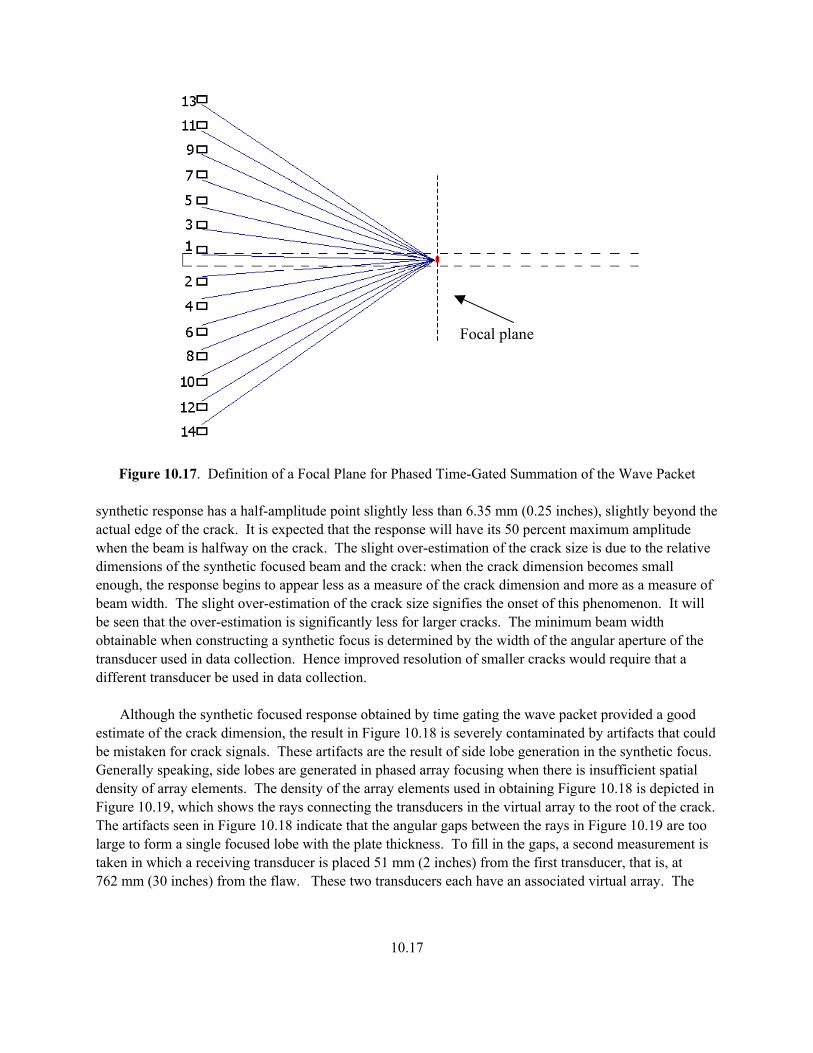
10.17

Focal plane

Figure 10.17. Definition of a Focal Plane for Phased Time-Gated Summation of the Wave Packet synthetic response has a half-amplitude point slightly less than 6.35 mm (0.25 inches), slightly beyond the actual edge of the crack. It is expected that the response will have its 50 percent maximum amplitude when the beam is halfway on the crack. The slight over-estimation of the crack size is due to the relative dimensions of the synthetic focused beam and the crack: when the crack dimension becomes small enough, the response begins to appear less as a measure of the crack dimension and more as a measure of beam width. The slight over-estimation of the crack size signifies the onset of this phenomenon. It will be seen that the over-estimation is significantly less for larger cracks. The minimum beam width obtainable when constructing a synthetic focus is determined by the width of the angular aperture of the transducer used in data collection. Hence improved resolution of smaller cracks would require that a different transducer be used in data collection. Although the synthetic focused response obtained by time gating the wave packet provided a good estimate of the crack dimension, the result in Figure 10.18 is severely contaminated by artifacts that could be mistaken for crack signals. These artifacts are the result of side lobe generation in the synthetic focus. Generally speaking, side lobes are generated in phased array focusing when there is insufficient spatial density of array elements. The density of the array elements used in obtaining Figure 10.18 is depicted in Figure 10.19, which shows the rays connecting the transducers in the virtual array to the root of the crack. The artifacts seen in Figure 10.18 indicate that the angular gaps between the rays in Figure 10.19 are too large to form a single focused lobe with the plate thickness. To fill in the gaps, a second measurement is taken in which a receiving transducer is placed 51 mm (2 inches) from the first transducer, that is, at 762 mm (30 inches) from the flaw. These two transducers each have an associated virtual array. The

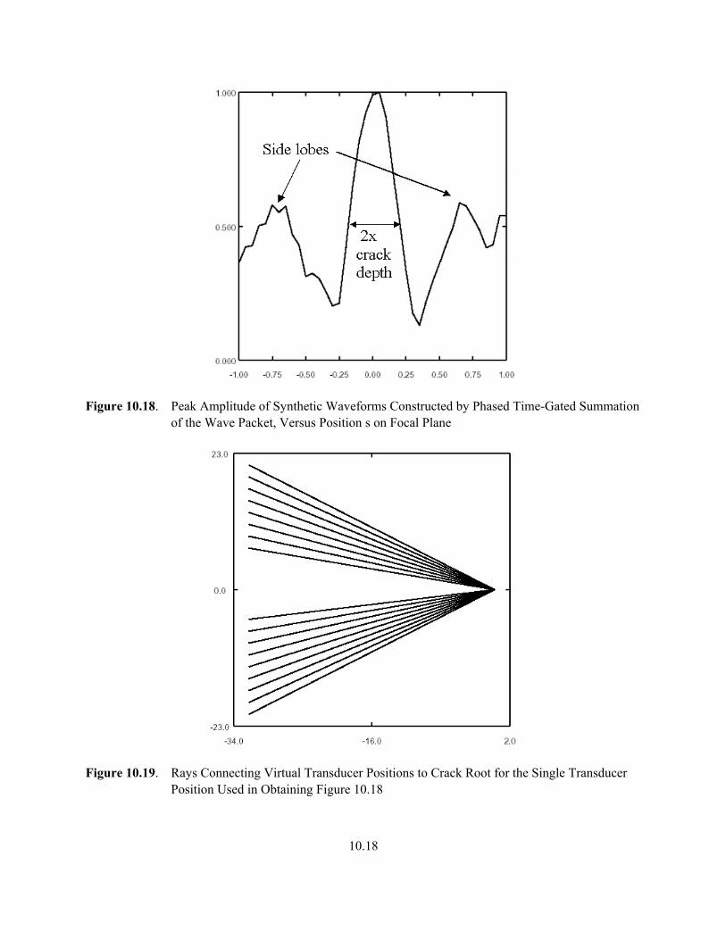
10.18

Figure 10.18. Peak Amplitude of Synthetic Waveforms Constructed by Phased Time-Gated Summation of the Wave Packet, Versus Position s on Focal Plane

Figure 10.19. Rays Connecting Virtual Transducer Positions to Crack Root for the Single Transducer

Position Used in Obtaining Figure 10.18

10.19

rays connecting the virtual array positions for the two transducers are shown in Figure 10.20. It is seen that the gaps observed in Figure 10.18 are filled in considerably. The synthetic focusing is now performed by wave packet gating of the pulse-echo signal from the first transducer, and the pitch-catch signal for transmission from the first transducer to the second transducer. Again, synthetic waveforms are constructed corresponding to each of the points of focus on the focal plane, and the peak amplitude of these signals is plotted versus position on the focal plane. The result of this two-transducer computation is shown in Figure 10.21. A significant reduction in side lobe-related artifacts is seen.

Figure 10.20. Rays Connecting Virtual Transducer Positions to Crack Root for Two Transducer

Positions Used in Obtaining Figure 10.21 The side lobe artifacts seen in Figure 10.21 can be reduced yet further by including a third measurement position. A result is shown in which a third transducer is employed, this time at a position 51 mm (2 inches) farther from the first transducer, or at 864 mm (34 inches) from the flaw. A plot of the rays connecting the virtual transducer positions to the root of the crack in this case is presented in Figure 10.22. The increased density in angular aperture coverage is evident. The crack response profile shown in Figure 10.23 correspondingly shows yet a further reduction in side lobe artifacts. It is evident that, at a distance of 813 mm (32 inches) to the flaw, accurate flaw sizing can be performed using two or three measurement positions, through exploitation of the virtual array properties of the high frequency guided wave signals. This observation could potentially translate into a significant reduction in the complexity of the in-situ data collection procedures. Since the procedure relies extensively on the properties of the virtual transducer array, it is proposed to refer to this procedure as “Virtual SAFT”, or V-SAFT, to distinguish it from the T-SAFT procedure incorporating one element of the virtual array.

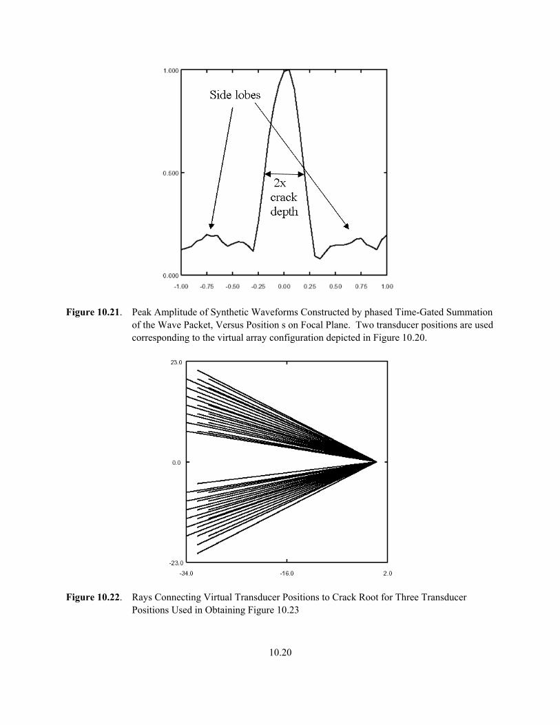
10.20

Figure 10.21. Peak Amplitude of Synthetic Waveforms Constructed by phased Time-Gated Summation

of the Wave Packet, Versus Position s on Focal Plane. Two transducer positions are used corresponding to the virtual array configuration depicted in Figure 10.20.

Figure 10.22. Rays Connecting Virtual Transducer Positions to Crack Root for Three Transducer Positions Used in Obtaining Figure 10.23

10.21

Figure 10.23. Peak Amplitude of Synthetic Waveforms Constructed by Phased Time-Gated Summation

of the Wave Packet, Versus Position s on Focal Plane. Three transducer positions are used corresponding to the virtual array configuration depicted in Figure 10.22.

Results are next presented comparing the V-SAFT response for cracks having depths of 5.1, 12.7, and 20.3 mm (0.2, 0.5, and 0.8 inches). The flaw sizing is performed using data collected from three transducer positions, identical to the procedure presented in Figure 10.23. The comparison, shown in Figure 10.24, only plots the response from s = 0 to s = 25.4 mm (s = 0 to s = 1 inch), corresponding to the physical dimension of the plate thickness. It is seen that the 50 percent amplitude points on the response curves agrees quite well with the dimension of the crack, particularly for the larger cracks (12.7 and 20.3 mm deep) (0.5 and 0.8 inch deep). Results are shown in Figure 10.25 for the case of cracks having depths of 5.1, 12.7, and 20.3 mm (0.2, 0.5, and 0.8 inches) that are extending from the outer wall of the plate, that is, the same side of the plate that the transducer is in contact with. It is seen that the results mirror those of Figure 10.24. This result indicates that it is in principle possible to discriminate between inner wall and outer wall cracking. It was demonstrated in Figures 10.18 through 10.23 how side lobe artifacts in the flaw reconstruction arise due to an insufficient array density, and how additional measurements can “fill in the gaps” in the SAFT data. It is interesting to note that another means increase the density in the sampling of the angular aperture is to increase the distance between the transducer and the flaw. The following example demonstrates this phenomenon. Figure 10.26 plots the rays connecting the virtual array transducer positions to the root of a 5.1 mm (0.2-inch) deep crack, for a transducer-to-flaw distance of 1778 mm

10.22

Figure 10.24. Peak Amplitude of Synthetic Waveforms Constructed by Phased Time-Gated Summation of

the Wave Packet, Versus Position s on Focal Plane. Results are compared for three different size cracks. Results were obtained using three transducer measurement positions.

Figure 10.25. Peak Amplitude of Synthetic Waveforms Constructed by Phased Time-Gated Summation

of the Wave Packet, Versus Position s on Focal Plane. Results are compared for three different size cracks, extending from the outside wall.

10.23

Figure 10.26. Rays Connecting Virtual Transducer Positions to Crack Root for the Single Transducer

Position Used in Obtaining Figure 10.28. Transducer-to-flaw distance is 1778 mm (70 inches).

(70 inches). The increased angular density of rays is apparent when compared to Figure 10.19. The signal obtained at 1778 mm (70 inches) in response to the 5.1 mm (0.2-inch) deep crack is plotted in Figure 10.27. The greater complexity of the signal, seen as the larger number of constituent components, reflects the greater ray density seen in Figure 10.26. The sizing of the crack estimated by time gating and phasing the components of this single wave packet is shown in Figure 10.28. The side lobe artifacts are observed to be substantially less severe than that observed in the single transducer result of Figure 10.18. This result demonstrates that it may be theoretically possible to perform flaw sizing using as few as one transducer measurement position. It is noted that the response in Figure 10.28 does not drop to zero for values of s greater than the dimension of the crack, but rather takes on a near constant value approximately 25 percent of the maximum. It is speculated that this is an effect of the accumulation of noise in the signal gating process. As was mentioned previously, there is no guarantee that only desired signals will fall within the selected time gate, and it is conceivable that undesired signals uniformly accumulate at all positions of s, resulting in an apparent “noise floor”. A similar phenomenon is seen to a lesser degree in the results obtained at 813 mm (32 inches). Because of the greater complexity seen in the signal of Figure 10.27, it stands to reason that there will be a corresponding increase in the level of gated noise. It is also noted that the over-estimation of the size of the crack is more severe in the result at 1778 mm (70 inches): the 50 percent amplitude point occurs at s = 7.4 mm (s = 0.29 inches). It is conceivable that this too is a consequence of noise accumulation in the sizing algorithm. More work is needed, however, to definitively explain these observations.

10.24

Figure 10.27. Wave packet for 20 Percent Through-Wall Crack for Transducer-to-Flaw Distance of

1778 mm (70 inches)

Figure 10.28. Peak Amplitude of Synthetic Waveforms Constructed by Phased Time-Gated Summation

of the Wave Packet, Versus Position s on Focal Plane. One transducer position is used corresponding to the virtual array configuration depicted in Figure 10.26.

10.25

Regarding the question motivating this study, “Does the wave packet contain information that could reduce the amount of data collection required to perform flaw sizing,” the results presented above indicate the answer is a definitive “yes”. The results suggest that flaw sizing might be performed with far fewer measurement positions, potentially simplifying the design of the crawler hardware, and significantly increasing scanning speed. The discoveries of this theoretical study point to possibilities to be examined in future development efforts. Questions to be examined in future development efforts include: 1) What is the robustness of the procedure? The sensitivity to input such as a priori knowledge of

distance to the flaw and shell thickness needs to be assessed. It would seem that sensitivity to these parameters would be no greater than that observed in the current T-SAFT procedure: indeed, the T-SAFT procedure differs only in that considers just one of the virtual array positions, and the robustness of the T-SAFT algorithm at long range has been thoroughly established. This suggests that if the available a priori data is adequate for one of the virtual array positions, it should be good enough for all.

2) How many data collection points are needed as a function of distance to the flaw? It was observed

that the density in the angular aperture sampling increases with distance between the transducer and flaw. Conversely, the density decreases as transducer-to-flaw distance decreases. The number of measurement positions required for a robust flaw sizing at various distances needs to be more thoroughly examined.

3) Is it possible to extend the V-SAFT procedure to the curved shell? This question is of utmost

importance to the tank knuckle inspection, and would be the highest priority item in a continued theoretical study of the measurement procedure. Considerable effort has been directed at this question this year, but conclusions are premature at this time. A significant problem introduced by the shell curvature is that, unlike the plate specimen, the virtual sources do not appear to be radiating point sources distributed throughout space, but rather appear to be extended radiating surfaces. Hence, computing a discrete travel time between the virtual source and the point of focus on the focal plane becomes problematic. There is reason to believe that these issues can be overcome. It is estimated that an additional effort comparable to this year’s effort should be sufficient to adequately explore this question.

10.2 Ray-Tracing Simulations at Pacific Northwest National Laboratory

(PNNL) This year the ray-tracing simulation work begun in 2001 was extended to provide pictorial ray traces, pulse-echo scan simulations, and T-SAFT scan simulations. Deficiencies in the software were corrected, and additional capabilities were added. These capabilities were used to help with interpretation of the acquired data. Some aspects of the simulations are shown pictorially. Figure 10.29 shows the user interface, as used for a pulse-echo trace simulation. In the left column (INPUTS) are the knuckle and transducer characteristics. The knuckle thickness and inside radius are input as 0.875 and 12 inches (22 and 305 mm) respectively. A transducer refracted beam angle of 70 degrees is assumed. A reflector is located at 127 mm (5 inches) inside the knuckle, on the inside

10.26

surface (Z equal to thickness). The remaining items in the left column are filled in automatically during the trace simulation. The second column (OUTPUTS) shows the last values of the last ray-trace during simulation. The third column has the scanning simulation parameters. The scan is performed from 279 mm (11 inches) above the weld to 25.4 mm (1 inch) above the weld. The transducer half-width beam angle is 10 degrees (from 60 to 80). The transducer coincidence size (5.1 mm) (0.1 inch) is used only for T-SAFT simulations. The three flaw emission angle range and step parameters control the number and range of rays that are used in the simulation. The flaw depth, X step, and X range are used only for T-SAFT. The simulation is performed by clicking the button marked “Generate Trace (Pulse-echo).” The results seen in the white box at bottom are the beginning of the output. The output is formatted with tabs and carriage returns to be pasted into a spreadsheet. Visualization of the results (shown in later figures) was performed in a spreadsheet, using X-Y graphing.

Figure 10.29. Pulse-Echo Trace Simulation Program, Set Up for Flaw at 127 mm (5 inches) in the

Knuckle, Scan From -279 to -25.4 mm (-11 to -1 inch) above the Knuckle

10.27

Figure 10.30 shows representative rays generated during a scan simulation, and two representative transducer positions during the simulation. The figure as shown was generated using the button marked “Generate Bounce Path” repeatedly (with different angle parameters) and combining the outputs into a single graph, along with data defining the shape of the knuckle, and line drawings to represent the transducer at two positions.

Figure 10.30. Representative Rays from Reflector at X=203 mm (X=8 inches) in the Knuckle, with

Transducer at two Possible Positions Near -51 and -152 mm (–2 and –6 inches)

10.28

Figure 10.31 shows two trace simulations overlaid. The dark blue trace, X=0, is at the transition from flat to curved, so the trace is the same as for any flat plate. The magenta curve, X=1.5, is 1.5 inch (38 mm) inside the curved region, and shows that even near the beginning of the curved region, the shape of the trace deviates substantially from the shape in a flat plate. This new curve can, in principle, be used to perform a modified SAFT algorithm within the curved region; time has not permitted an implementation of that possibility.

X=1.5

X=0

Figure 10.31. Simulated Knuckle Trace at 38 mm (1.5 inch) Overlaid with Simulated Flat-Plate Trace

at the Same Distance Figure 10.32 shows data from 254 mm (10-inch) into the curved region (dark blue trace) overlaid with data from a 254 mm (10-inch) distance in a flat plate (magenta). Three aspects of this stand out. First, there are multiple traces, resulting from the multiple bounce paths in a plate geometry (flat or curved). Second, the flat plate shows three large traces and one small trace, while the curved region shows only two large traces, with a few data points occurring near the small flat-plate trace. Third, the slopes and curvatures of the flat and curved traces are markedly different.

10.29

Flat Plate Trace

Figure 10.32. Simulated Pulse-Echo Traces From Knuckle at 254 mm (10 inches) Overlaid With

Simulated Traces in Flat Plate at 254 mm (10 inches) Figure 10.33 shows a simulated T-SAFT scan, optimized for a flaw at 127 mm (5 inches) in the curved region. To generate this, the button marked “Generate Trace (T_SAFT)” was clicked (with different parameters than those shown in the earlier figure). In this figure, the two colors represent the two halves of the scan. The dark blue shows the points with the sending transducer beyond the central point and the receiving transducer closer than the central point. The magenta shows the points with the sending transducer closer than the central point and the receiving transducer beyond the central point. The asymmetry between the two colors results from the difference in paths taken by the rays as they propagate through the transition from curved to straight region of the knuckle. The different layers of traces result from the different multiple-bounce paths that the sound can take over a long distance in a plate (flat or curved). In a flat plate, the width of the trace is equal to twice the depth of the flaw times the sine of the beam angle. In the knuckle geometry, the curved-to-flat transition can increase or decrease the trace width, making flaw sizing more difficult. In this example, the width is increased by about a factor of two – the simulated flaw depth was 7.6 mm (0.3 inch), and the simulated measured flaw depth, using 70 degrees as the appropriate angle, is 7.6 mm (0.7 inch). Using this simulation at the detected flaw position, and adjusting the data interpretation accordingly, may enhance the ability to size flaws.

10.30

Unprojected DataX=5, Z=0.875, N=5

10

10.5

11

11.5

12

12.5

13

-8 -7 -6 -5 -4 -3 -2 -1 0

Expected path 10.630

Figure 10.33. Simulated T-SAFT Traces at X = 127 mm (X = 5) Inches in the Knuckle, Inner Surface Figure 10.34 shows actual pulse-echo data overlaid with simulated pulse-echo data. The fit between the data sets was made visually rather than analytically. The fit of the first few traces is quite good, but it gets worse for the later traces. An interesting aspect of these displays is the difference between inner and outer surface reflectors. This difference was noted at various X positions in the curved region. In the outer surface picture (left) there are several strong reflections grouped together at the upper left, and the traces are somewhat irregular, with a small trace following the first trace. In the inside surface picture (right) there is just one strong reflector, and the traces are smooth curves. Analysis of the ray paths indicates that the difference results from the rays that travel around the outer surface of the curved region without reflecting from the inside surface.

10.31

Figure 10.34. Actual Pulse-Echo Data at 432 mm (17 inches) in the Knuckle (colors), Overlaid with

Simulated Traces (in white). The left-hand picture is from a reflector on the outer surface, the right, on the inner surface at the same X location.

11.1

11.0 FY02 Demonstrations and Training Training of the NDE operator on the RONDE system took place in September FY02. The training consisted mostly of hands on work, learning the software menus and understanding the principals of the T-SAFT method of flaw characterization. Shown in Figure 11.1 is the NDE Ultrasonic Level III performing an inspection of a mockup at a PNNL facility. Once the training was completed, the NDE Level III participated in a performance demonstration test of the RONDE system.

Figure 11.1. NDE Level III completing Performance Demonstration Testing The SAFT/T-SAFT scanner is shown in Figure 11.2 attached to the magnetic wheel crawler used to position the scanner on one of PNNL’s mockups. Two demonstrations were performed in FY02 to show the capability of the SRAIV system. The first demonstration was provided to SRS personnel who observed the operation of the T-SAFT scanning bridge connected to the SRS (Force Institute) crawler. PNNL deployed the entire crawler and T-SAFT scanning bridge through a simulated 127 mm (5 in.) riser to show clearance requirements. A second demonstration of the SRAIV system was performed for DOE-RL, CH2M Hill Hanford Group, and PNNL management.

11.2

Figure 11.2. SAFT/T-SAFT Scanner

Figure 11.3. Greg Dyches from SRS Observes the Operation of the SRAIV

11.3

Figure 11.4. TFA Manager Mike Terry Observes the SRAIV Operation

12.1

12.0 Conclusions The design, development, and performance testing of a prototype system known as the RONDE system to examine the knuckle region of a DST have been completed. Data gathered this year demonstrated the prototype system’s capability utilizing a combination of pitch-catch SAFT and tandem-SAFT inspection methodologies to perform flaw detection, localization and sizing in the knuckle region. PNNL designed and fabricated a SAFT scanning bridge for SRS. This scanning bridge was coupled to an existing SRS crawler and the completed system was designated as the SRAIV system. Initial testing was performed to demonstrate the system’s capability for deployment and data acquisition. The system was successfully demonstrated to SRS personnel. In support of the prototype system testing and performance demonstrations, a mockup was fabricated containing real intergranular stress corrosion cracking. This mockup proved invaluable in providing evidence that the RONDE system could detect and size real cracks in the knuckle region of Hanford’s waste tanks. This mockup also contains IGSCC beyond the knuckle extending under the tank floor. PNNL demonstrated that real IGSCC can be detected under the tank as well if the need arises. Equipment qualification and performance testing of the RONDE system have been completed. All required defects in all of the mockups including the IGSCC mockup were readily detected. The NDE Level III Ultrasonic inspector assigned to this project sized all of the detected flaws in the knuckle region of both the sawcut and IGSCC mockups. His sizing results are shown below: 12.1 Machined Defects Sizing The accuracy requirement for depth sizing of machined defects is a root mean square (RMS) value of 2.54 mm (0.1 in.). Figure 12.1 is a plot of the data provided by NDE Level III Ultrasonic inspector Mr. Wes Nelson. Mr. Nelson’s RMS value for all machined defects is 1.4 mm (0.055 in.), well below the 2.54 mm (0.1 in.) criteria.

Wes Nelson Sawcuts

0

0.2

0.4

0.6

0 0.5 1

UT Measured Data

True

Sta

te D

ata

PerfectPerformance

UT MeasuredData

Figure 12.1. Sizing Results on Machined Sawcuts

12.2

12.2 Inter-Granular Stress Corrosion Cracks (IGSCC) The requirement for sizing IGSCC is the same as the requirement for the machined defects, namely 2.54 mm (0.1 in.). Figure 12.2 is the plot of the data provided by Mr. Nelson. The RMS value of this data is 1.8 mm (0.07 in.), which is well within the 2.54 mm (0.1 in.) requirements.

Wes Nelson Cracks

00.20.40.60.8

0 0.2 0.4 0.6 0.8

UT Measured Data

Truc

e St

ate

Dat

a

UT MeasuredDataPerfectPerformance

Figure 12.2. Sizing Results on IGSCC

13.1

13.0 FY 03 Plans 13.1 RONDE Deployment into a Hanford Waste Tank It is anticipated that the RONDE system will be ready for deployment into the annulus of a DST in the 1st quarter of FY03. PNNL plans to support the deployment and assist NDE inspectors during the data acquisition and interpretation. 13.2 SRAIV-SAFT FY03 Plans The initial prototype SRAIV-SAFT scanning bridge will be available for further testing and enhancements in FY03. It will up to SRS personnel to fund further development and testing and deployment into a SRS waste tank annulus.

14.1

14.0 References Auld, B.A. 1979. General Electromechanical Reciprocity Relations Applied To The Calculation of Elastic Wave Scattering Coefficients, Wave Motion 1, pp. 3-10. Busse, L. J., H. D. Collins, and S. R. Doctor. 1984. Review and Discussion of the Development of Synthetic Aperture Focusing Technique for Ultrasonic Testing (SAFT-UT), NUREG/CR-3625. U.S. Nuclear Regulatory Commission, Washington, D.C. Hall, T. E., L. D. Reid, and S. R. Doctor. 1988. The SAFT-UT Real-Time Inspection System - Operational Principles and Implementation, NUREG/CR-5075. U.S. Nuclear Regulatory Commission, Washington, D.C. Jensen, C. E., 2001. Engineering Task Plan for the Ultrasonic Inspection of Hanford Double-Shell Tanks-FY2001, RPP-6839, CH2M Hill Hanford Group, Inc., Richland, Washington. Pardini, A. F., et al. 2001. Annual Report – Development of a Remotely Operated NDE System for Inspection of Hanford’s Double Shell Waste Tank Knuckle Regions, PNNL-13682, Pacific Northwest National Laboratory, Richland, Washington. Pardini, A. F., and T. J. Samuel. 2001. Functions and Requirements for the DST Knuckle Region Ultrasonic Scanning System, PNNL-13436, Pacific Northwest National Laboratory, Richland, Washington. Pfluger, D. C. 1994. Double-Shell Tank Ultrasonic Inspection Plan, WHC-SD- WM-AP-019, Westinghouse Hanford Company, Richland, Washington. Pfluger, D. C. 1995. Double-Shell Tank Ultrasonic Inspection Performance Specification, WHC-S-4108, Westinghouse Hanford Company, Richland, Washington. Roberts, R. A., A. F. Pardini, and A. A. Diaz. 2001. A Model for High Frequency Guided Wave Inspection of Curved Shells, Review of Progress in Quantitative NDE, Bowdoin College, Brunswick, Maine, July 29-August 3, 2001. Shurrab, M. S., M. D. Thomson, J. R. Friley, M. R. Garnich, M. W. Rinker and F. A. Simonen. 1991. Parametric Studies to Support Inspection Criteria of the Hanford Site Double-Shell Waste Storage Tanks, WHC-EP-0508, Westinghouse Hanford Company, Richland, Washington. Wong, J. W., G. M. Dyches, A. F. Pardini. 2001. Functions and Requirements for the Small Roving Annulus Inspection Vehicle (U), WSRC-MS-2001-00557, Westinghouse Savannah River Company, Aiken, South Carolina.

Distr-1

Distribution No. of Copies Offsite 4 DOE/Office of Scientific and Technical Information & Information Release 1 DOE Office of Science and

Technology Kurt Gerdes 1154 Cloverleaf Building 19901 Germantown Road Germantown, MD 20874-1290

Onsite 8 Tanks Focus Area Technical Team B. J. Williams K9-69 1 Tanks Focus Area Program Manager T. P. Pietrok K8-50 1 Tanks Focus Area - Safety M. T. Terry K9-91 1 Hanford Site E. J. Cruz H6-60 30 Pacific Northwest National Laboratory

J. M. Alzheimer (1) K5-22 L. O. Casazza (1) K5-26 S. L. Crawford (1) K5-26 A. A. Diaz (1) K5-26 S. R. Doctor (1) K5-26 K. L. Gervais (1) K5-22 R. V. Harris (1) K5-26 A. F. Pardini (16) K5-26 G. J. Posakony (1) K5-26 T. J. Samuel (5) K5-22 G. J. Schuster (1) K5-26