Annular Modes of Variability in the Atmospheres of Mars and Titan

J. Michael Battalio* and Juan M. Lora

Department of Earth and Planetary Sciences

Yale University

210 Whitney Ave.

New Haven, CT 06511

*Corresponding Author: michael@battalio.com

Annular modes explain much of the internal variability of Earth’s atmosphere but have

never been identified on other planets. Using reanalyses for Mars and a simulation for Ti-

tan, we demonstrate that annular modes are prominent in the atmospheres of both worlds,

explaining large fractions of their respective variabilities. One mode describes latitudinal

shifts of the jet on Mars, as on Earth, and vertical shifts of the jet on Titan. Another de-

scribes pulses of midlatitude eddy kinetic energy on all three worlds, albeit with somewhat

different characteristics. We further demonstrate that this latter mode has predictive pow-

er for regional dust activity on Mars, revealing its usefulness for understanding Martian

weather. In addition, our finding of similar annular variability in dynamically diverse

worlds indicates its ubiquity across planetary atmospheres, opening a new avenue for com-

parative planetology as well as an additional consideration for characterization of extraso-

lar atmospheres.

Annular modes arise from the internal dynamics of the atmosphere1,2. In Earth’s atmosphere,

they explain much of the weekly to monthly variability of the jet stream, synoptic wave activity,

and precipitation3–10 so are vital to understanding and predicting weather patterns. They are

linked to the position and strength of the jet stream and atmospheric storm track. Modes are

“annular” if the variability they represent is zonally symmetric—that is, if changes occur in tan-

dem along whole latitude circles11. Two types of annular modes exist within the atmosphere of

Earth. The first mode arises as north-south vacillations (quantified as the first empirical orthog-

onal function [EOF]; see Methods) in the anomalous surface pressure1,3 or zonal-mean zonal

wind4,6. This mode appears independently in both the northern and southern hemispheres, in

each case explaining 20–30% of the variance in the zonal-mean wind, geopotential height, and

surface pressure1. The mode physically represents shifts in atmospheric mass between the polar

regions and the middle latitudes. (The second EOF of the zonal-mean wind, representing the

next most variance, describes strengthening of the jet in place6,12.) The vertical uniformity of the

wind signature and importance of momentum fluxes associated with this mode indicate it is a

barotropic feature4,6,8,13,14. The second type of annular mode—the Baroclinic Annular Mode—

dominates the variance of zonal-mean eddy kinetic energy (henceforth EKE) and also appears in

both the northern and southern hemispheres, explaining 43% and 34%, respectively, of the EKE

variance8,14,15. This mode associates with anomalous eddy heat fluxes and varies with height,

indicating a baroclinic nature.

The importance of annular variability on Mars was heretofore thought to be minimal16,17, despite

Mars having similar atmospheric dynamics18, atmospheric energy cycles19, baroclinic wave life-

cycles20–22, and semiannual oscillation23 as Earth. Conversely, Titan inhabits a different regime

of atmospheric dynamics, with a high Rossby number24 (though near-surface baroclinic waves

occur in simulations of Titan’s atmosphere25–28). Motivated by the possibility that annular modes

may help diagnose and predict weather on other planets as they do for Earth, we investigate if

annular modes—including searching for baroclinic modes for the first time—are present on Mars

and Titan. This would indicate their ubiquity in terrestrial atmospheres and reveal an important

common source of atmospheric variability for consideration on both Solar System and extrasolar

planets.

The purportedly inconsequential influence of barotropic annular modes on Mars16,17 belied issues

with the horizontal weighting of the analyzed fields (see Methods). The seemingly minor change

to the correct weighting has enormous impacts on the resulting importance of annular modes on

Mars. Using EOF analysis with the correct weighting, we identify both baroclinic and barotropic

annular modes on Mars and Titan and also compare them to Earth’s modes. For Mars, we focus

on each hemisphere’s fall and winter seasons and analyze two reanalysis datasets, the Mars

Analysis Correction Data Assimilation (MACDA)29 and the Ensemble Mars Atmosphere Re-

analysis System (EMARS)30. For Titan, we evaluate the full year using simulations from the Ti-

tan Atmosphere Model31.

Martian annular mode in zonal wind

Indeed, our EOF analysis of the atmosphere of Mars (see Methods) demonstrates many annular

features reminiscent to those on Earth. Much of the large-scale variability of the mid-to-high

latitude atmospheric flow is explained by an annular mode in the zonal-mean zonal wind (hence-

forth U-AM) (Fig. 1a–d and Extended Data Fig. 2a–d). In addition, we identify for the first time

an annular mode in the zonal-mean EKE (EKE-AM) on another planet (Fig. 2a–d). These modes

are the equivalents of Earth’s barotropic (Fig 3 of ref. 4, Fig. 2a of ref. 6, Fig. 2a of refs. 8, 14)

and baroclinic (Fig. 2f of refs. 8, 14) annular modes, respectively.

Two spatial structures dominate the variability of Mars’s zonal-mean zonal wind. A dipolar

structure—which is equivalent to Earth’s U-AM—straddles the region of strongest winds (annu-

al-mean zonal wind contoured in Fig. 1a–d) and explains the most variance in the northern hemi-

sphere (~30–40%, Fig. 1b, d). As on Earth, the dipolar pattern represents latitudinal shifts of the

jet. Because topography in the southern hemisphere varies greatly with latitude, such north-

south shifts are disrupted, and additional spatial structures are also important in that hemisphere:

A mono-polar structure—with a single center of action—accounts for slightly more variance

(~25–35%, Extended Data Fig. 2a, c) than the dipolar structure (~20–30%, Fig. 1a, c), indicating

that both are similarly important. Regardless, the spatial locations of the dipolar modes (Fig. 1a–

d) align in both hemispheres and across datasets, with positive centers at 70º N/S and negative

centers at approximately 40º N/S, all at around 100 Pa (approximately 20 km altitude), indicating

that the spatial pattern is robust.

The dipolar U-AM behaves like Earth's U-AM, which links to eddy momentum fluxes and lacks

any tilt in the vertical—a barotropic structure. This inter-planetary similarity of the barotropic

mode is revealed by regressing the eddy momentum fluxes onto the U-AM at a -1 day lag (Fig.

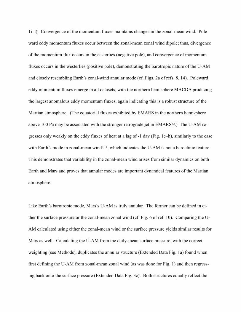
1i–l). Convergence of the momentum fluxes maintains changes in the zonal-mean wind. Pole-

ward eddy momentum fluxes occur between the zonal-mean zonal wind dipole; thus, divergence

of the momentum flux occurs in the easterlies (negative pole), and convergence of momentum

fluxes occurs in the westerlies (positive pole), demonstrating the barotropic nature of the U-AM

and closely resembling Earth’s zonal-wind annular mode (cf. Figs. 2a of refs. 8, 14). Poleward

eddy momentum fluxes emerge in all datasets, with the northern hemisphere MACDA producing

the largest anomalous eddy momentum fluxes, again indicating this is a robust structure of the

Martian atmosphere. (The equatorial fluxes exhibited by EMARS in the northern hemisphere

above 100 Pa may be associated with the stronger retrograde jet in EMARS32.) The U-AM re-

gresses only weakly on the eddy fluxes of heat at a lag of -1 day (Fig. 1e–h), similarly to the case

with Earth’s mode in zonal-mean wind8,14, which indicates the U-AM is not a baroclinic feature.

This demonstrates that variability in the zonal-mean wind arises from similar dynamics on both

Earth and Mars and proves that annular modes are important dynamical features of the Martian

atmosphere.

Like Earth’s barotropic mode, Mars’s U-AM is truly annular. The former can be defined in ei-

ther the surface pressure or the zonal-mean zonal wind (cf. Fig. 6 of ref. 10). Comparing the U-

AM calculated using either the zonal-mean wind or the surface pressure yields similar results for

Mars as well. Calculating the U-AM from the daily-mean surface pressure, with the correct

weighting (see Methods), duplicates the annular structure (Extended Data Fig. 1a) found when

first defining the U-AM from zonal-mean zonal wind (as was done for Fig. 1) and then regress-

ing back onto the surface pressure (Extended Data Fig. 3c). Both structures equally reflect the

movement of mass away from the pole at times of westerly anomalies in the jet. If this analysis

is repeated with an incorrect horizontal weighting, the annular structure is relegated to EOF 3, as

in previous work16,17 (Extended Data Fig. 1f). Thus, as on Earth, the methods for defining the U-

AM on Mars, using either the zonal-mean winds or the surface pressure, are equivalent.

Martian annular mode in eddy kinetic energy

Just as the U-AM resembles Earth’s barotropic mode, the newly-identified Martian EKE-AM

resembles Earth’s baroclinic annular mode (cf. Figs. 2f of ref. 8, 14, and Fig. 1 of ref. 15). The

first spatial pattern is a single monopole that overlaps the greatest EKE and explains between 48

and 65% of the EKE variance (Fig. 2a–d), far larger than for Earth8,14. The location of the re-

gressed zonal-mean EKE matches that of Earth’s baroclinic mode, but the magnitude of the

EKE-AM is approximately double. The annular feature achieves a maximum at 60–70º N/S and

10–150 Pa and is robust across both hemispheres and both datasets. Given the large degree of

importance Earth’s mode has in explaining extratropical wave activity, the comparatively larger

percentage of variance explained by the EKE-AM points to its immense influence in determining

wave activity, and therefore dust events33, on Mars.

The EKE-AM links to poleward eddy heat fluxes that vary vertically (Fig. 2e–h), which matches

the behavior of Earth’s baroclinic mode and demonstrates that the EKE-AM represents (baroclin-

ic) instabilities that instigate the type of traveling waves that initiate large dust events33. The re-

lationship between eddy heat fluxes and the EKE-AM holds across hemispheres and datasets ex-

cepting the southern hemisphere MACDA domain, wherein fluxes are weaker. Nevertheless,

each domain exhibits a peak in the magnitude of eddy heat fluxes near the surface in the midlati-

tudes, with a secondary peak around 100 Pa slanted poleward and passing through the maximum

of the EKE (Fig. 2e–h, contours).

Earth’s baroclinic and barotropic annular modes are decoupled, meaning that there is essentially

no correlation between them; they act independently of one another. Additionally, Earth’s mode

in EKE is not linked to eddy fluxes of momentum, and Earth’s mode in zonal wind is not linked

to eddy fluxes of heat8,14. The Martian U-AM follows this pattern, as it does not regress strongly

on either eddy heat fluxes or EKE (Fig. 1e–h). However, this is not the case for the Martian

EKE-AM: The EKE-AM is associated with eddy fluxes of momentum (Fig. 2i–l) that are ap-

proximately double those related to the U-AM (Fig. 1i–l), though the EKE-AM does not regress

on zonal-mean zonal wind (Fig. 2i–l, contours). This is distinctly different from Earth’s EKE-

AM8,14; thus, the Martian EKE-AM cannot be established as strictly a baroclinic mode. The en-

tangled nature of Martian annular modes corroborates wave analyses22 that find that transient

eddies grow barotropically as well as baroclinically, depending on the period of the dominant

waves. Thus, while annular modes on Mars are quite similar to those of Earth, the unique condi-

tions of Mars provide some intriguing differences that demand continued investigation.

The connections between the EKE-AM and dust storm-producing traveling waves on Mars are

corroborated by comparing the storm tracks on Mars to the EKE-AM. The mass-integrated

EKE33, which is a measure of the intensity of waves, regressed on the EKE-AM peaks at 45–75º

N and 15–60º S (Fig. 3c, d). It connects to the EKE-AM upstream of Acidalia, Arcadia, and

Utopia Planitiae in the northern hemisphere, and near Argyre and Hellas Basins in the southern

hemisphere, with only minor disagreements in magnitude between datasets (Extended Data Fig.

3e–h). Indeed, each of these regions hosts areas of increased storm activity from transient

waves22,33,34,40. Furthermore, the clear annular structure, with longitudinal localization in storm

tracks, is remarkably reminiscent of Earth’s EKE-AM, which also pinpoints the Pacific, Atlantic,

and Southern Ocean storm tracks (Fig. 3a, b)8,14,15. The similarity in the annular modes in EKE

on both Earth and Mars therefore suggests that the EKE-AM may be essential for midlatitude

weather on Mars.

Impact of Martian annular modes on dust activity

Earth’s annular modes link to observable and impactful atmospheric features, like precipitation15,

further implying that the newfound EKE-AM might be expected to impact observable Martian

weather like dust activity. To probe the link between the northern hemisphere EKE-AM and dust

activity, we regress the EKE-AM onto the Mars Dust Activity Database35 for the dusty season of

one Mars year. Regions where northern hemisphere dust storms initiate, like Acidalia, Utopia, or

Arcadia Planitae, are highlighted when dust activity leads the EKE-AM in the regression (Fig.

4a), demonstrating a relationship between the mode and observable, impactful surface conditions

on Mars. That the EKE-AM pinpoints regions related to dust storm activity in an independent

dataset also increases the confidence that annular modes on Mars truly exist. In these three re-

gions in the northern hemisphere, dust activity peaks before the EKE-AM, meaning that dust is

lifted and begins to be transported by atmospheric waves before the waves reach their peak in-

tensity. This is analogous to the relationship between Earth’s EKE-AM and precipitation, where

precipitation peaks one day before waves do15.

A key difference between precipitation on Earth and dust on Mars is that the latter remains lofted

for weeks after initially being lifted. Thus, with Mars, the impact of the EKE-AM remains long

after the peak of the EKE itself. In fact, when the dust activity lags the EKE-AM (i.e., the EKE-

AM peak precedes the dust), locations into which northern hemisphere dust storms evolve—or

flush33,35,36—link positively to the northern EKE-AM (Fig. 4b). This relationship between the

northern EKE-AM and southern hemisphere dust activity maximizes near 0.12 storms/sol be-

tween Argyre and Hellas Basins, which is the region into which most dust storms travel33,35.

Therefore, the leading behavior of the EKE-AM for activity that moves from the north to the

south indicates predictive abilities of annular modes for dust storms. Only those dust events that

flush into the southern midlatitudes become large enough to impact the surrounding atmos-

phere33, so the EKE-AM could indicate when large dust events are favored before they occur.

These sorts of predictions could be vital, for example, to ensuring the safety of future crewed

missions to Mars.

Titan’s annular modes

We have shown that Earth and Mars share similar annular modes in zonal wind and EKE, which

could be due to their similarity in dynamical regime. To test this, we also investigate annular

modes on Titan, which presents a heretofore unexplored dynamical regime from the perspective

of annular variability. With key differences from Earth and Mars, Titan, too, supports annular

modes of variability in zonal-mean zonal wind and EKE, based on simulations with a Titan gen-

eral circulation model31 (no reanalysis exists yet for Titan; see Methods). While potentially in-

augurating additional research into Titan’s atmospheric variability, these analyses should be in-

terpreted with caution since they are from a single, albeit well-validated26,27,31, model. Never-

theless, evidence of annular modes on Titan, in addition to Earth and Mars, points to the ubiquity

of annular variability across the Solar System, which may hold significant promise for under-

standing atmospheric behavior across worlds.

The U-AM in our Titan simulations is dipolar but with the opposing poles stacked vertically (Fig.

5a, b) instead of horizontally like on Earth or Mars. Titan’s U-AM explains ~68% of the vari-

ance of the zonal-mean zonal wind, far more than for Earth or Mars. The negative pole resides at

300 hPa (approximately 30 km altitude), while the weaker positive pole resides near the lowest

vertical extent of the jet: This spatial structure represents vertical oscillations of the jet, as op-

posed to the horizontal vacillations of the terrestrial and Martian U-AM. Titan’s U-AM is char-

acterized by co-located zonal wind and poleward momentum fluxes (Fig. 5i, j). There is little

relationship between the U-AM and EKE, but the U-AM is associated with poleward heat fluxes

near the surface and equatorward heat fluxes in the mid-levels (Fig. 5e, f). Despite the vertical

alignment of the U-AM dipole, the mode is associated with low surface pressures at the pole and

an annular feature between 30 and 45º N/S in the anomalous mass-integrated EKE (not shown),

which may indicate that the waves associated with the EKE have barotropic components, in

agreement with expectations for Titan’s dynamical regime37. This is counter to the nature of the

terrestrial and Martian U-AM.

Titan’s EKE-AM, though similar to Mars’s and Earth’s modes, also provides intriguing differ-

ences. Titan’s EKE-AM explains 38.5 and 52% of the southern and northern hemisphere vari-

ance, respectively, in the zonal-mean EKE and has a single center of action at 500 hPa and 60º

N/S (Fig. 5c, d). However, this mode exhibits a vertically stacked dipole of eddy heat fluxes that

are poleward at high altitudes and equatorward in the mid-levels. These equatorward eddy heat

fluxes indicate that the waves generating the EKE cannot be baroclinic in the mid-levels of the

atmosphere38. Additionally, the EKE-AM regresses only weakly on the zonal wind (Fig. 5k, l,

contours), similarly to Earth’s baroclinic mode, but links strongly to eddy momentum fluxes

(Fig. 5k, l), like the Martian EKE-AM (Fig. 2). Titan’s annular modes, therefore, share charac-

teristics of both Earth’s and Mars’s modes. Whether they too have predictive power for weather

on Titan remains to be explored.

Implications and Perspectives

Previous studies suggested that annular variability might be unimportant in the atmosphere of

Mars16,17; however, we find that annular variability is even more important on Mars than it is on

Earth. The northern and southern Martian modes explain larger percentages of variance in the

zonal wind than Earth’s U-AM (Fig. 1). And, for the first time, we identify a baroclinic annular

mode in the EKE on Mars and on Titan as well, both of which explain almost double the amount

of variance in EKE—and thus wave activity—compared to Earth’s baroclinic mode.

That Mars and Titan both exemplify annular variability opens a new window for comparative

planetology and climatology. Mars’s modes are more similar to Earth’s, but the possible modes

of Titan demonstrate how the influence of differing planetary parameters modifies the atmos-

pheric dynamics. Annular structure in the EKE-AM occurs on Earth, Mars, and Titan between

35 and 65º N/S as seen in mass-integrated EKE (Fig. 3). These six fields are strikingly similar

given the disparate topographies, storm tracks, and—particularly for Titan—dynamical regimes

of the three worlds. Mars’s EKE-AM amplifies within the three northern21,34,39 and two south-

ern22,40 storm tracks that generate dust activity (Fig. 3c,d). Titan’s EKE-AM controls EKE

throughout an annulus between 35 and 60º N/S, and activity is most strongly indicated in the

northern hemisphere between 180 and 300º E (Fig. 3e, f), suggesting that there may be preferred

locations for eddy activity as on Earth and Mars. In addition to longitudinal localization of the

storm tracks for Earth and Mars, mass-integrated EKE is dramatically amplified throughout the

mid-latitudes on all three worlds (Fig. 3).

An exciting application lies in the use of annular dynamics to explain observable phenomena on

Mars, Titan, and elsewhere. Annular modes on Earth link to the distribution of precipitation15,

cloud cover9, and trace atmospheric species5,7. For Mars, dust is the most important visible con-

sequence of changing weather patterns, and the Martian EKE-AM indeed exhibits a strong link

to dust activity (Fig. 4). Further, the high degree of annularity of the Martian polar vortex32 may

relate to the relatively more important Martian U-AM and EKE-AM. In addition, connecting the

EKE-AM to dust activity, and thus atmospheric temperatures41, provides a physical (as opposed

to a dynamical12) coupling to the Martian U-AM via changes in the surface pressure by sublima-

tion/deposition of the CO2 seasonal ice cap. For Titan, annular modes may play a role in the spo-

radic nature convective events42, but further observations and improved model simulations will

be required to assess their relationship.

Finally, the existence of annular modes in atmospheres other than Earth’s proves the ubiquity of

annular modes of variability across planetary atmospheres and demands a search for these modes

beyond Mars and Titan. For example, Venus exhibits annularity in the “cold collar” of tempera-

tures surrounding the pole43; this may link to annular variability as Earth’s annular modes link to

low temperatures8. Given this ubiquity, annular variability might be expected in gas and ice gi-

ants as well, for instance given the likely importance of eddies in driving Jupiter’s jets44. Annu-

lar modes might also impart intrinsic variability that sets the noise floor for detections of exo-

planet winds via Doppler shifts45 so should be understood in that context. Each of these possibil-

ities opens a promising avenue of research toward understanding how annular dynamics controls

observable variability in the atmospheres of Earth and other planets.

References

1. Thompson, D. W. & Wallace, J. M. Annular modes in the extratropical circulation. Part I: Month-to- month variability. Journal of Climate 13, 1000–1016 (2000).

2. Hassanzadeh, P. & Kuang, Z. Quantifying the Annular Mode Dynamics in an Idealized At-mosphere. Journal of the Atmospheric Sciences 76, 1107–1124 (2019). 1809.01054.

3. Trenberth, K. E. & Paolino Jr., D. A. Characteristic Patterns of Variability of Sea Level Pres-sure in the Northern Hemisphere. Monthly Weather Review 109, 1169–1189 (1981).

4. Hartmann, D. L. & Lo, F. Wave-driven zonal flow vacillation in the Southern Hemisphere. Journal of the Atmospheric Sciences 55, 1303–1315 (1998).

5. Hartmann, D. L., Wallace, J. M., Limpasuvan, V., Thompson, D. W. & Holton, J. R. Can ozone depletion and global warming interact to produce rapid climate change? Proceedings of the National Academy of Sciences of the United States of America 97, 1412–1417 (2000).

6. Lorenz, D. J. & Hartmann, D. L. Eddy-Zonal Flow Feedback in the Southern Hemisphere. Journal of the Atmospheric Sciences 58, 3312–3327 (2001).

7. Butler, A. H., Thompson, D. W. & Gurney, K. R. Observed relationships between the Southern Annular Mode and atmospheric carbon dioxide. Global Biogeochemical Cycles 21, 1–8 (2007).

8. Thompson, D. W. J. & Woodworth, J. D. Barotropic and Baroclinic Annular Variability in the Southern Hemisphere. Journal of the Atmospheric Sciences 71, 1480–1493 (2014).

9. Li, Y. & Thompson, D. W. J. Observed signatures of the barotropic and baroclinic annular modes in cloud vertical structure and cloud radiative effects. Journal of Climate 29, 4723–4740 (2016).

10. Thompson, D. W. J. & Wallace, J. M. The Arctic oscillation signature in the wintertime geopotential height and temperature fields. Geophysical Research Letters 25, 1297–1300 (1998).

11. Gerber, E. P. & Thompson, D. W. J. What Makes an Annular Mode “Annular”? Journal of the Atmospheric Sciences 74, 317–332 (2017).

12.Boljka, L., Shepherd, T. G. & Blackburn, M. On the coupling between barotropic and baro-clinic modes of extratropical atmospheric variability. Journal of the Atmospheric Sciences 75, 1853–1871 (2018).

13. Limpasuvan, V. & Hartmann, D. L. Wave-Maintained Annular Modes of Climate Variability. Journal of Climate 13, 4414–4429 (2000).

14. Thompson, D. W. J. & Li, Y. Baroclinic and Barotropic Annular Variability in the Northern Hemisphere. Journal of the Atmospheric Sciences 72, 1117–1136 (2015).

15.Thompson, D. W. J. & Barnes, E. A. Periodic Variability in the Large-Scale Southern Hemi-sphere Atmospheric Circulation. Science 343, 641–645 (2014).

16.Leroy, S. S., Yung, Y. L., Richardson, M. I. & Wilson, R. J. Principal modes of variability of Martian atmospheric surface pressure. Geophysical Research Letters 30, 1–4 (2003).

17. Yamashita, Y., Kuroda, T. & Takahashi, M. Maintenance of zonal wind variability associated with the annular mode on Mars. Geophysical Research Letters 34, 2–6 (2007).

18. Barnes, J. R. et al. The Global Circulation, in The Atmosphere and Climate of Mars, 229–294. Cambridge Planetary Science (Cambridge University Press, 2017).

19. Tabataba-Vakili, F. et al. A Lorenz/Boer energy budget for the atmosphere of Mars from a “reanalysis” of spacecraft observations. Geophysical Research Letters 42, 8320–8327 (2015).

20. Greybush, S. J., Kalnay, E., Hoffman, M. J. & Wilson, R. J. Identifying martian atmospheric instabilities and their physical origins using bred vectors. Quarterly Journal of the Royal Me-teorological Society 139, 639–653 (2013).

21. Battalio, M., Szunyogh, I. & Lemmon, M. Energetics of the martian atmosphere using the Mars Analysis Correction Data Assimilation (MACDA) dataset. Icarus 276, 1–20 (2016).

22. Battalio, M., Szunyogh, I. & Lemmon, M. Wave energetics of the southern hemisphere of Mars. Icarus 309, 220–240 (2018).

23. Ruan, T., Lewis, N. T., Lewis, S. R., Montabone, L. & Read, P. L. Investigating the semian-nual oscillation on Mars using data assimilation. Icarus 333, 404–414 (2019).

24. Mitchell, Jonathan L., and Juan M. Lora. “The Climate of Titan.” Annual Review of Earth and Planetary Sciences 44, no. 1 (2016): 353–80.

25. Lora, J. M., & Mitchell, J. L. Titan’s Asymmetric Lake Distribution Mediated by Methane Transport due to Atmospheric Eddies. Geophysical Research Letters 42, 6213–6220 (2015).

26. Faulk, S. P., Mitchell, J. L., Moon, S. & Lora, J. M. Regional patterns of extreme precipita-tion on Titan consistent with observed alluvial fan distribution. Nature Geoscience 10, 827–831 (2017).

27. Lora, J. M., Tokano, T., Vatant d’Ollone, J., Lebonnois, S. & Lorenz, R. D. A model inter-comparison of Titan’s climate and low-latitude environment. Icarus 333, 113–126 (2019).

28. Lebonnois, S., Burgalat, J., Rannou, P. & Charnay, B. Titan global climate model: A new 3-dimensional version of the IPSL Titan GCM. Icarus 218, 707–722 (2012).

29. Montabone, L. et al. The Mars Analysis Correction Data Assimilation (MACDA) Dataset V1.0. Geoscience Data Journal 1, 129–139 (2014).

30. Greybush, S. J. et al. The Ensemble Mars Atmosphere Reanalysis System (EMARS) Version 1.0. Geoscience Data Journal 1–14 (2019).

31. Lora, J. M., Lunine, J. I. & Russell, J. L. GCM simulations of Titan’s middle and lower at-mosphere and comparison to observations. Icarus 250, 516–528 (2015). 1412.7995.

32. Waugh, D. W. et al. Martian polar vortices: Comparison of reanalyses. Journal of Geophysi-cal Research: Planets 121, 1–16 (2016).

33. Battalio, M. & Wang, H. Eddy evolution during large dust storms. Icarus 338, 113507 (2020).

34. Hollingsworth, J. L. et al. Orographic Control of Storm Zones on Mars. Nature 380, 413–16 (1996).

35.Battalio, M., & Wang, H. The Mars Dust Activity Database (MDAD): A comprehensive sta-tistical study of dust storm sequences. Icarus, 354, 114059 (2021).

36.Wang, H. & Richardson, M. I. The Origin, Evolution, and Trajectory of Large Dust Storms on Mars during Mars Years 24–30 (1999–2011). Icarus 251, 112–127 (2015).

37.Rossow, W. B. & Williams, G. P. Large-Scale Motion in the Venus Stratosphere. Journal of the Atmospheric Sciences 36, 377–389 (1979).

38.Charney, J. G. The Dynamics of Long Waves in a Baroclinic Westerly Current. Journal of Meteorology 4 (1947).

39.Mooring, T. A. & Wilson, R. J. Transient eddies in the MACDA Mars reanalysis. Journal of Geophysical Research: Planets 120, 1–26 (2015).

40.Battalio, M. & Wang, H. The Aonia-Solis-Valles dust storm track in the southern hemisphere of Mars. Icarus 321, 367–378 (2019).

41.Kass, D. M. et al. Interannual similarity in the martian atmosphere during the dust storm sea-son. Geophysical Research Letters 43 (2016).

42.Schaller, E. L., Brown, M. E., Roe, H. G., & Bouchez, A. H.. A large cloud outburst at Titan’s south pole. Icarus, 182 (1), 224–229 (2006).

43.Ando, H. et al. The puzzling Venusian polar atmospheric structure reproduced by a general circulation model. Nature Communications, 7, 1–8 (2016).

44.Williams, G. P. Jovian Dynamics. Part III: Multiple, Migrating, and Equatorial Jets. Journal of Atmospheric Sciences, 60 (10), 1270–1296 (2003).

45.Snellen, I. A. G., et al. The orbital motion, absolute mass and high-altitude winds of exoplan-et HD 209458b. Nature, 465 (7301), 1049–1051 (2010).

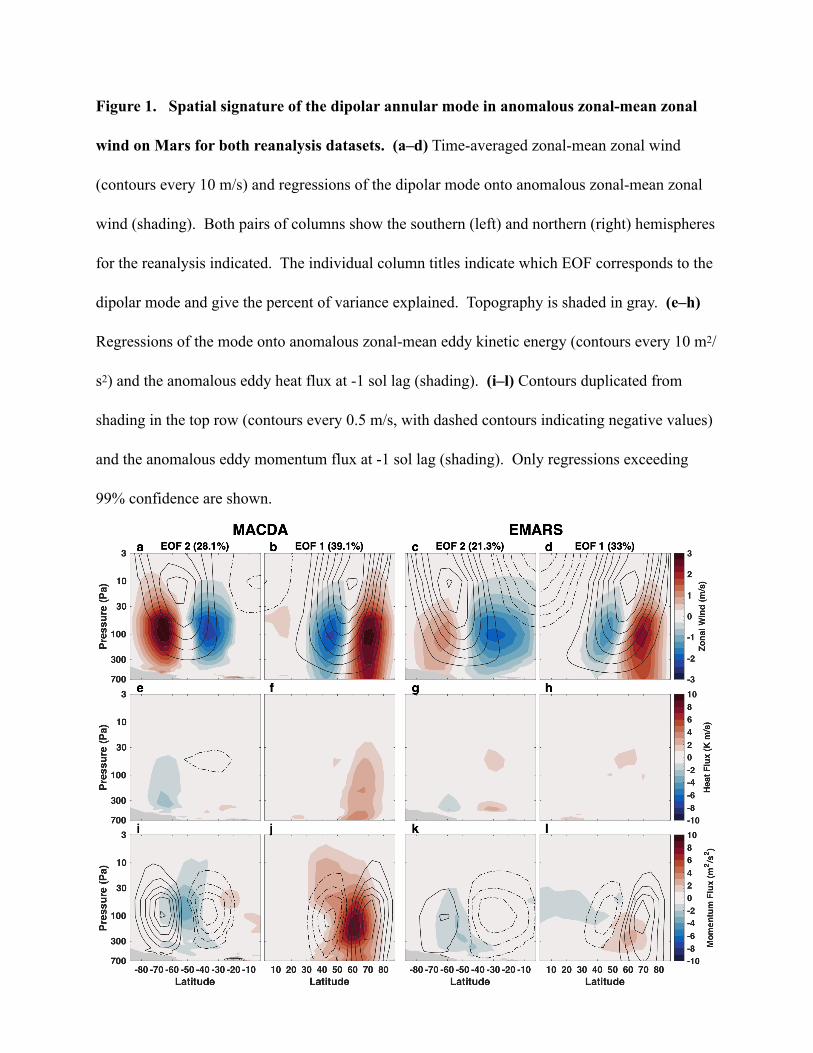
Figure 1. Spatial signature of the dipolar annular mode in anomalous zonal-mean zonal

wind on Mars for both reanalysis datasets. (a–d) Time-averaged zonal-mean zonal wind

(contours every 10 m/s) and regressions of the dipolar mode onto anomalous zonal-mean zonal

wind (shading). Both pairs of columns show the southern (left) and northern (right) hemispheres

for the reanalysis indicated. The individual column titles indicate which EOF corresponds to the

dipolar mode and give the percent of variance explained. Topography is shaded in gray. (e–h)

Regressions of the mode onto anomalous zonal-mean eddy kinetic energy (contours every 10 m2/

s2) and the anomalous eddy heat flux at -1 sol lag (shading). (i–l) Contours duplicated from

shading in the top row (contours every 0.5 m/s, with dashed contours indicating negative values)

and the anomalous eddy momentum flux at -1 sol lag (shading). Only regressions exceeding

99% confidence are shown.

Figure 2. Spatial signature of the first annular mode in anomalous zonal-mean eddy kinet-

ic energy on Mars for both reanalysis datasets. (a–d) As in Fig. 1 but for the time-averaged

zonal-mean eddy kinetic energy (contours every 200 m2/s2) and regressions onto the anomalous

zonal-mean eddy kinetic energy (shading). (e–h) Contours duplicated from shading in the top

row (contours every 10 m2/s2) and the anomalous eddy heat flux at 0 sol lag (shading). (i–l) Re-

gressions of the mode onto zonal-mean zonal wind (contours every 0.5 m/s with dashed contours

indicating negative values) and the anomalous eddy momentum flux at 0 sol lag (shading). Re-

gressions are only shown exceeding 99% confidence.

Figure 3. Polar plots of vertically (mass) integrated EKE regressed onto the EKE-AM for

Earth (a, b), Mars (c, d), and Titan (e, f). (a, c, e) Northern hemisphere. (b, d, f) Southern

hemisphere. For Mars, topography is shown in 2000 m increments with the 0 m contour dot-

dashed in gray and negative contours dashed. Regressions are only shown exceeding 99% con-

fidence.

Figure 4. Regression of the EKE-AM from the EMARS northern hemisphere on the Mars

Dust Activity Database for Mars Year 31. (a) dust activity leading the EKE-AM by 4 sols. (b)

dust activity lagging the EKE-AM by 4 sols. Regressions are performed on the Mars dusty sea-

son (Ls=180–360º) and are only shown exceeding 95% confidence. Topography is shown in

2000 m increments with the 0 m contour and negative contours dot-dashed.

Figure 5. Zonal-mean structure of the annular modes in zonal-mean zonal wind (left two

columns) and eddy kinetic energy (right two columns) on Titan. (a, b) Dataset-averaged

zonal-mean zonal wind (contours every 5 m/s) and regression of the U-AM onto the zonal-mean

wind (shading). (c, d) Dataset-averaged zonal-mean eddy kinetic energy (contours every 5x10-2

m2/s2) and regression of the EKE-AM onto the zonal-mean eddy kinetic energy (shading). The

individual column titles give the percent of variance explained. (e–h) Regressions onto the

anomalous zonal-mean eddy kinetic energy (contours every 2.5x10-2 m2/s2) and the anomalous

eddy heat flux at 0 day lag (shading) for the U-AM (e, f) and for the EKE-AM (g, h). (i–l) Re-

gressions onto the anomalous zonal-mean zonal wind (contours every 5x10-2 m/s) and anomalous

eddy momentum flux at -1 day lag for the U-AM (i, j) and for the EKE-AM (k, l). Regressions

are only shown exceeding 99% confidence.

Methods

We perform an empirical orthogonal function analysis of annular structures of variability in the

atmosphere of Mars using two reanalysis datasets, the Mars Analysis Correction Data Assimila-

tion (MACDA)29 and the Ensemble Mars Atmospheric Reanalysis System (EMARS). The latter

consists of two eras, during which Thermal Emission Spectrometer data and Mars Climate

Sounder data are assimilated, respectively30. We conduct a similar analysis for Titan using a 20

Titan-year-long simulation of the Titan Atmospheric Model (TAM)31. We use the ERA-Interim

reanalysis for Earth data46.

Time of Year on Mars

Timekeeping on Mars is related to the position of the planet in its orbit. The seasons on Mars are

delineated using the areocentric longitude, Ls, which ranges from Ls = 0–360º. For the northern

hemisphere, vernal equinox is Ls = 0º, summer solstice is Ls = 90º, autumnal equinox is Ls =

180º, and winter solstice is Ls = 270º.

Mars Reanalysis Datasets

MACDA (v1.0)29 is a reanalysis of Thermal Emission Spectrometer retrievals47 from the Mars

Global Surveyor during the period Ls = 141º MY 24 to Ls = 86º MY 27. Thermal profiles up to

40 km twice per sol and total dust opacities once per sol are assimilated into the UK version of

the LMD Mars Global Circulation Model48 using an analysis correction scheme49. MACDA uses

a 5º × 5º horizontal grid with 25 sigma levels every two Mars hours.

EMARS (v1.0)30 includes Thermal Emission Spectrometer data, as well as assimilations from the

Mars Climate Sounder50 onboard the Mars Reconnaissance Orbiter; thus, EMARS spans from Ls

= 103º MY 24 to Ls = 102º MY 27 using the Thermal Emission Spectrometer, and Ls = 112º MY

28 to Ls = 105º MY 33 using the Mars Climate Sounder30. EMARS is provided at 6º longitude ×

5º latitude horizontal resolution with 28 hybrid sigma-pressure levels. EMARS uses a Local En-

semble Transform Kalman Filter to assimilate observations51,52.

EMARS is an ensemble dataset, meaning that the model is run multiple times with different pa-

rameterizations to characterize the “true” synoptic state of the atmosphere as observed. Thus, the

ensemble mean is used for the analysis. We favor the use of the ensemble mean as opposed to

the use of an individual member because we seek to understand the most likely state of the at-

mosphere as opposed to a deterministic diagnosis from one model. For the Thermal Emission

Spectrometer era, the ensemble has been shown to generally converge to a single solution when

analyzing transient waves, but for Mars Climate Sounder data, surface features are less con-

strained52. Nevertheless, repeating our analysis on a single ensemble member from EMARS

does not change our results (not shown).

Titan Atmospheric Model

Though Mars research has benefitted from semi-continuous and regular observations of its at-

mosphere over several Martian years, Titan’s long year and relative distance have prevented con-

tinuous monitoring for any substantial length of time: The recent Cassini mission only sporadi-

cally observed Titan during its tour of the Saturn system, which covered half of a Titan year.

Given this relative dearth of observational data and a lack of reanalysis products for Titan, the

next best option is an observationally benchmarked general circulation model.

Therefore, to explore the possibility of annular modes on Titan, we turn to an analysis of simula-

tions of Titan’s atmosphere with TAM31.

A 20 Titan-year simulation is re-initialized from a previously reported TAM simulation53—which

includes the atmospheric model coupled to a land model incorporating interactive hydrology—

using the preferred version with a surface hydraulic conductivity of k=5 x 10-5 m/s, which

matches best to observations of the hydrologic cycle. TAM has been thoroughly vetted against

numerous observations of Titan, and its simulated circulation has been shown to be ro-

bust26,27,31,54, as well as favorably comparable to other models of Titan’s climate27,28,55. Neverthe-

less, the Titan analyses herein are of a single model, so should be interpreted with caution.

Empirical orthogonal function analysis

Earth’s annular modes are diagnosed using empirical orthogonal function (EOF) analysis3,56,57.

We adopt a similar methodology for Mars and Titan to identify the leading patterns of annular

climatic variability. EOF analysis decomposes a time series of data into multiple functions (of

the same spatial dimensions as the analyzed dataset) that are determined by statistical relation-

ships within the dataset. EOFs are the eigenvectors of the covariance matrix at each grid point

and time step. The eigenvalue associated with each EOF eigenvector corresponds to the variance

that is accounted for by the EOF. These functions are orthogonal, meaning they most efficiently

represent the variance of the entire dataset. Each EOF of the dataset is paired with a principal

component (PC) time series (of the same length as the original dataset). This principal compo-

nent describes the temporal evolution/amplitude of the EOF at every time step of the dataset3.

The EOFs and associated PCs are ordered such that the first EOF explains the largest amount of

variance of the original field; each subsequent EOF explains the largest amount of remaining

variance3.

The EOFs shown in the analysis are tested for significance, defined as their being well-separated

from adjacent modes56. This is estimated using the formula , where N is

the number of timesteps and is the eigenvalue for each mode56. For all reanalysis domains for

Mars and for the TAM simulation, all first modes are well-separated from the second modes, and

all second modes are well-separated from the third modes.

The annular modes are defined using the zonal-mean zonal wind [u] and zonal-mean eddy kinet-

ic energy , where square brackets denote the zonal mean, and aster-

isks indicate departures from the zonal mean. The eddy momentum flux and eddy

meridional heat flux are also considered. Eddies and fluxes are calculated at each out-

put time step within MACDA or EMARS and then averaged over each sol. Eddies and fluxes

are calculated within TAM at each model time step (600 seconds) and averaged over an output

frequency of approximately 0.9 Titan days.

For the Martian U-AM, we differentiate spatial structures as dipolar or non-dipolar modes. The

non-dipolar U-AM on Mars (Extended Data Fig. 2) explains marginally more variance in the

δλα = λα4(2/N )1/2

λa

[EKE ] = [u*2 + v*2]/2

[u*v*]

[v*T*]

southern hemisphere than the dipolar mode (Fig. 1). The additional mode is tri-polar in MACDA

(Extended Data Fig. 2a, b) signifying splitting of the jet and mono-polar in the southern hemi-

sphere in EMARS (Extended Data Fig. 2c) representing intensification of the jet. These varia-

tions in structure for both the first and second EOFs are not uncommon for Earth8,12 and may

represent differences in the representation of the jet between reanalyses. The regressed momen-

tum fluxes are colocated with a center of regressed zonal wind (Extended Data Fig. 2i–l). This

does not correspond to a barotropic mode and is therefore not considered further.

Anomalies defined from the seasonal average

In most studies of Earth’s annular modes, EOF analysis is performed on anomalies that are de-

fined by subtracting the seasonal cycle from each year. For this method to successfully approxi-

mate the real seasonal cycle, the dataset must be of a long enough duration that a single year with

large anomalies does not influence the averaged yearly cycle. For Mars, an analysis performed

on anomalies defined from a seasonal average is dominated by the effects of the global dust

storms in MY 25 and 28 and to a lesser extent the regional storms that occur each fall and win-

ter41 (not shown). This induces anomalies that are not real being defined in the years without a

global dust storm. The only way to ameliorate the issue is to approximate the seasonal average

by filtering out long-period temporal signals using a low-pass filtered time series, to balance cap-

turing the seasonal cycle with removing shorter-period perturbations. A Hamming window filter

with a cutoff of 100 Mars or Titan days is used in our analyses. For the EMARS dataset, using

the seasonal cycle on the years without a global dust storm (MY 29–33) compared to the full

climatology using the filtering procedure provides similar results (not shown) with a correlation

of the PC and EOF to the full MY 28–33 EMARS dataset r=0.998. Combined with the finding

that the spatial patterns of variability during global dust storms are highly correlated to the pat-

terns without global storms (r≥0.95), this indicates that global dust storms merely amplify exist-

ing spatial patterns of annular variability instead of generating additional modes (see below on

Regression of Principal Components).

Sensitivity to domain size

For Mars, we analyze the daily mean of each variable over the domain 700–1 Pa and 0–90º N/S

for the [EKE] and 18–90º N/S for the [u]. The EOF structure of the EKE-AM for Mars is robust

as domain size is changed. The spatial structure of the Martian U-AM remains unchanged when

the domain size is decreased; however, if the domain of analysis is increased to the equator, an

additional mode is revealed within the EMARS datasets that represents strengthening and weak-

ening of the retrograde jet at the equator, which is stronger for large portions of the year in

EMARS compared to MACDA32. For Titan, we analyze fields from the surface (around 1450

hPa) to the top of the model domain at 0.05 hPa and over the range 8–90º N/S. The TAM results

are insensitive to changes in the domain size in the meridional direction, spanning up to 30º de-

grees and to changes in the vertical direction to as low as 100 hPa. For both Mars and Titan, the

southern and northern hemispheres are analyzed separately.

Weighting in the meridional direction

Before performing the EOF analysis, the Mars reanalysis data are converted to pressure coordi-

nates in the vertical direction. All data are weighted by mass vertically and weighted in the

meridional direction by a factor of , where is latitude. Previous efforts to describe

annular variability in the atmosphere of Mars using the surface pressure, weighted by ,

demoted the annular modes of variability to the third EOF16,17. The use of an inappropriate

weighting ( ) in the meridional direction also relegates Earth’s barotropic annular mode in

geopotential height to the third EOF, while weighting with places the annular mode as

the leading EOF58. Applying our EOF analysis of surface pressure from EMARS on incorrectly

weighted ( ) anomalous, daily mean surface pressure also shows the most prominent annu-

lar mode in the third EOF (Extended Data Fig. 1f), whereas the appropriately weighted (

), anomalous, daily mean surface pressure from EMARS yields a regression map with

an annular mode in EOF 1 (Extended Data Fig. 1a). The factor is used because vari-

ance, which is what is assessed in EOF analysis, is a squared quantity58 (see Extended Data Fig.

1a versus 1b).

One complexity for Mars is the deposition and sublimation of the CO2 ice cap, which breaks the

relationship between the shift of the zonal wind maximum and mass: for the times of year where

the CO2 ice cap is changing, atmospheric mass is not conserved. Indeed, the second spatial

structure of the U-AM defined from the surface pressure is not annular (Extended Data Fig. 1b),

despite the equivalent structure being annular when defined from the zonal-mean zonal wind (not

shown). Thus, care must be taken when comparing the U-AM calculated from either the winds

or the surface pressure.

cosϕ ϕ

cosϕ

cosϕ

cosϕ

cosϕ

cosϕ

cosϕ

Regression of Principal Components

The spatial patterns produced by EOF analysis indicate the locations of action of the annular

modes but do not indicate the locations where the modes most impact variables of interest. To

ascertain these links, we regress the anomaly fields (of zonal wind, momentum flux, surface

pressure, etc.) onto the associated standardized leading PC to generate maps of the regression.

The PCs are standardized by dividing each by its standard deviation. This is preferred because

standardized PC time series are unitless, so the regressed maps have the same units as the anom-

aly field itself 1. The resulting maps correspond to anomalies in the regressed field that are asso-

ciated with variations in the PC. We assess the significance of regression coefficients with the t

statistic. The number of degrees of freedom used in the test of significance is computed from the

lag-1 autocorrelation59. Throughout the work, the level of significance is noted in the text and

figure captions, and results are never reported below the 95% confidence level.

For the U-AM on Titan, we regress the eddy momentum fluxes at a lag of -1 day. For the U-AM

on Mars, we regress the eddy momentum and eddy heat fluxes at a lag of -1 sol, following terres-

trial results6. For the EKE-AM, we regress all fluxes for both Mars and Titan at a lag of zero, as

the fluxes maximize coincident with the PCs.

For the Titan results, we regress the entire PC time series onto each field of interest. For the

Mars reanalysis datasets, we do not regress during the periods of global dust storms (MY 25,

Ls=170–300º and MY 28, Ls=260–325º), due to the large, transient impact on wind and tempera-

ture fields. To ensure that the annular modes themselves are not simply artifacts of the global

dust storms, we have repeated our analyses excluding the global dust storms entirely. This yields

five periods of comparison: before the MY 25 global dust event for MACDA and EMARS, after

the MY 25 global dust event for MACDA and EMARS, and after the MY 28 global dust event

for EMARS. Each of the EOFs and PCs for both annular modes are correlated to the full run of

the analysis at r≥0.95. This implies that the global dust storms merely amplify the annular

modes of variability themselves instead of imposing new patterns of variability.

Dust storms flush from the northern to the southern hemispheres during northern autumn and

winter33,35,36. So, to prevent inter-hemispheric dynamics from impacting the interpretation of the

annular modes, we only present results where we regress the PCs for the northern hemisphere for

the period Ls=180–370º and the southern hemisphere for Ls=10–190º. These periods correspond

to the times of the strongest transient wave activity in each hemisphere60.

Mars Dust Activity Database

Observations of Martian dust storm activity are taken from the Mars Dust Activity Database

(MDAD)35,61. Each Mars Color Imager, Mars Daily Global Map36 covers 90º N–90º S. The pe-

riod Ls=180–360º, which is typically considered the dust storm season35, from MY 31 is used.

The MDAD notes all dust storm activity with well-defined boundaries on Mars with area >105

km2 and indicates each storm individually with an ID number. Dust storms with well-defined

boundaries are easily identified from Mars Daily Global Maps, with the edges of the dust storms

manually outlined35. For comparison to the EKE-AM, the MDAD is re-binned from 0.1º × 0.1º

resolution to 1º × 1º resolution, and all of the dust storms on each sol are collected together. The

resulting array is regressed against the EKE-AM just as other fields taken directly from the re-

analysis datasets.

Methods References

46. Uppala, S. et al. The ERA-40 re-analysis Quarterly Journal of the Royal Meteorological So-ciety 131, 2961–3012 (2005).

47. Smith, M. D. Interannual variability in TES atmospheric observations of Mars during 1999-2003. Icarus 167, 148–165 (2004).

48. Forget, F. et al. Improved general circulation models of the martian atmosphere from the sur-face to above 80 km. Journal of Geophysical Research 104, 24155 (1999).

49. Lewis, S. R., Read, P. L., Conrath, B. J., Pearl, J. C. & Smith, M. D. Assimilation of thermal emission spectrometer atmospheric data during the Mars Global Surveyor aerobraking period. Icarus 192, 327–347 (2007).

50. Kleinböhl, A. et al. Mars Climate Sounder limb profile retrieval of atmospheric temperature, pressure, and dust and water ice opacity. Journal of Geophysical Research: Planets 114, 1–30 (2009).

51. Greybush, S. J. et al. Ensemble Kalman filter data assimilation of Thermal Emission Spec-trometer temperature retrievals into a Mars GCM. Journal of Geophysical Research 117, E11008 (2012).

52. Greybush, S. J., Gillespie, H. E. & Wilson, R. J. Transient eddies in the TES/MCS Ensemble Mars Atmosphere Reanalysis System (EMARS). Icarus 317, 158–181 (2019).

53. Faulk, S. P., Lora, J. M., Mitchell, J. L. & Milly, P. C. D. Titan’s climate patterns and surface methane distribution due to the coupling of land hydrology and atmosphere. Nature Astrono-my (2019).

54. Lora, J. M. & Ádámkovics, M. The near-surface methane humidity on Titan. Icarus 286, 270–279 (2017).

55.Newman, C. E., Richardson, M. I., Lian, Y. & Lee, C. Simulating Titan’s methane cycle with the TitanWRF General Circulation Model. Icarus 267, 106–134 (2016).

56. North, G. R., Bell, T. L. & Cahalan, R. F. Sampling Errors in the Estimation of Empirical Or-thogonal Functions. Monthly Weather Review 110, 699–706 (1982).

57. Greene, C. et al. The Climate Data Toolbox for MATLAB. Geochemistry, Geophysics, Geosystems 20 3774–3781 (2019).

58. Chung, C. & Nigam, S. Weighting of geophysical data in Principal Component Analysis. Journal of Geophysical Research 104, 16925–16928 (1999).

59.Bretherton, C. S., Widmann, M., Dymnikov, V. P., Wallace, J. M. & Bladé, I. The effective number of spatial degrees of freedom of a time-varying field. Journal of Climate 12, 1990–2009 (1999).

60.Lewis, S. R. et al. The solsticial pause on Mars: 1. A planetary wave reanalysis. Icarus 264, 456–464 (2016).

61. Battalio, M. & Wang, H. The Mars Dust Activity Database (MDAD). Harvard Dataverse (2019), doi: 10.7910/DVN/F8R2JX.

Correspondence and requests for materials should be addressed to J. Michael Battalio

(michael@battalio.com).

Data Availability

The Mars Analysis Correction Data Assimilation is available at https://catalogue.ceda.ac.uk/uuid/

01c44fb05fbd6e428efbd57969a11177. The Ensemble Mars Atmospheric Reanalysis System is

available at ftp://ftp.pasda.psu.edu/pub/commons/meteorology/greybush/emars-1p0/data/. ERA-Inter-

im data are available at https://www.ecmwf.int. The Mars Dust Activity Database is available at

https://doi.org/10.7910/DVN/F8R2JX. Titan Atmospheric Model results will be archived on Zeno-

do or similar.

Code Availability

The source code for TAM is currently not publicly available. EOF analysis was done in part

with the Climate Data Toolbox for Matlab (https://github.com/chadagreene/CDT). Other scripts

used in the study can be obtained from the corresponding author upon request.

Author Contributions

J.M.B. conceived of the work. J.M.B. performed the analysis and wrote the manuscript, with

contributions from J.M.L. J.M.L. ran simulations of TAM.

Competing Interest declaration

The authors declare no competing interests.

Extended Data Figures

Extended Data Figure 1. Polar plots of the regression of the first three EOFs onto the

anomalous surface pressure from EMARS in the northern hemisphere. (a, c, e) results per-

formed using weighting of . (b, d, f) results using . The individual panel titles

indicate the percent of variance explained in each EOF. Topography is shown in 2000 m incre-

ments with the 0 m contour dot-dashed in gray and negative contours dashed. Regressions are

only shown exceeding 99% confidence.

cosϕ cosϕ

Extended Data Figure 2. The spatial signature of the first non-dipolar annular mode in

anomalous zonal-mean zonal wind on Mars for both reanalysis datasets. (a–l) As in Fig. 1,

but for the first non-dipolar U-AM.

Extended Data Figure 3. Polar plots of the regression of the Martian U-AM onto the anom-

alous surface pressure (a–d) and the regression of the Martian EKE-AM onto the anom-

alous, vertically (mass) integrated EKE (e–h). (a, c, e, g) MACDA. (b, d, f, h) EMARS.

Topography is shown in 2000 m increments with the 0 m contour dot-dashed in gray and nega-

tive contours dashed. Regressions are only shown exceeding 99% confidence.