anomalous and significant subgraph detection in attributed...

Anomalous and Significant Subgraph Detection in Attributed Networks

Part II: Dynamic networks

Feng Chen 1, Petko Bogdanov 1, Daniel B. Neill 2, and Ambuj K. Singh 3

Department of Computer ScienceCollege of Engineering and Applied SciencesUniversity at Albany - SUNY

1

H.J. Heinz III CollegeCarnegie Mellon University

Department of Computer Science & Biomolecular Science and Engineering University of California at Santa Barbara

2

3

1

Roadmap

• Introduction & Motivation

• Part 1: Subgraph Detection in Statistic Attributed Networks

• Part 2: Subgraph Detection in Dynamic Attributed Networks

• Future Directions

2

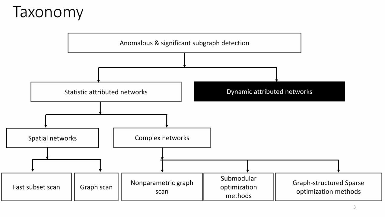
Taxonomy

Anomalous & significant subgraph detection

Statistic attributed networks Dynamic attributed networks

Fast subset scan

Complex networksSpatial networks

Graph scanNonparametric graph

scan

Submodular optimization

methods

Graph-structured Sparse optimization methods

3

Specifics of the dynamic setting

• Graph and temporal (multi-network) dimensions• Graph: Connectivity/Density/Weight• Time: Contiguity/Recurrence/Stability

• Baseline: Independent snapshot detection and then connect in time• (-) Do not consider all slices at a time• (-) Heuristic post-processing across time

• Focus for this part: detection of general subgraphs

• What we will NOT address• Global network properties over time• Individual node/edge properties over time• Evolutionary clustering: partitions the full network as

opposed to focus on specific subgraphs• Static structure: e.g. community detection

India

NCT

Pakistan

NCT

New

Zealand

NCT

Sri

Lanka

NCT

Cricket

Pages

India

NCT

Pakistan

NCT

New

Zealand

NCT

Sri

Lanka

NCT

Cricket

Pages

NZ Cricket

Players

India

NCT

Pakistan

NCT

New

Zealand

NCT

Sri

Lanka

NCT

Cricket

Pages

India

NCT

Pakistan

NCT

Sri

Lanka

NCT

28/3 29/3

30/3 - 31/3

Cricket

Pages

1/4 - 4/4

India

NCT

Cricket

Pages

5/4

2011 Cricket World Cup

Finals Schedule

4

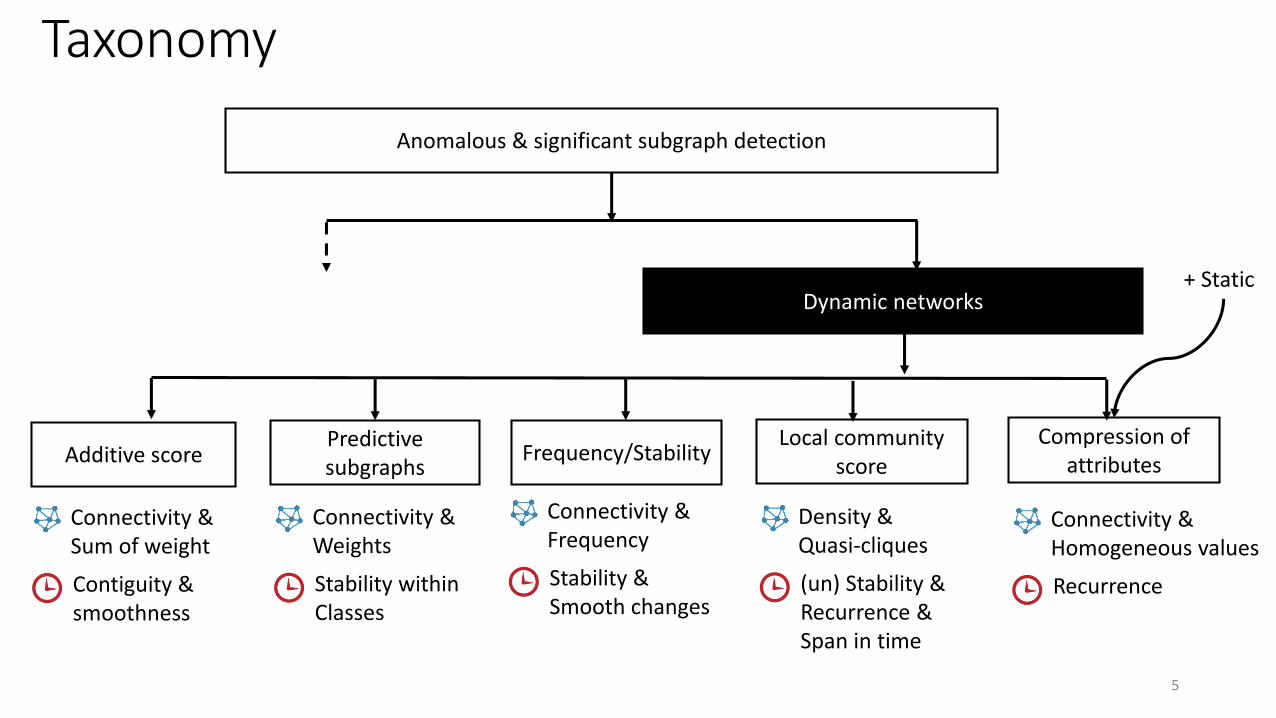
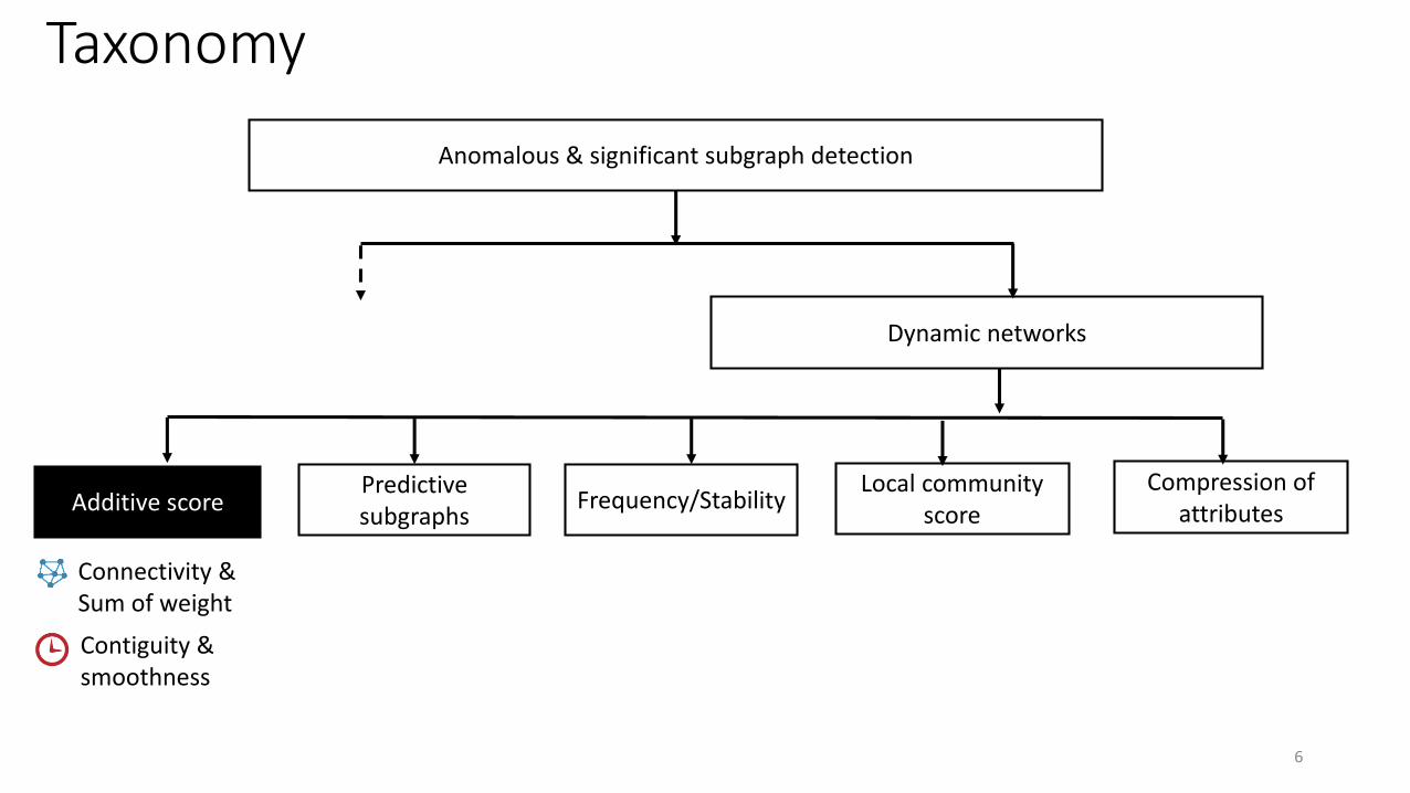
Taxonomy


Dynamic networks

Predictive subgraphs

Additive score Frequency/StabilityLocal community

score

Compression of attributes

+ Static

5

Connectivity &Sum of weight

Contiguity &smoothness

Connectivity &Weights

Stability withinClasses

Connectivity &Frequency

Stability & Smooth changes

Density &Quasi-cliques

(un) Stability & Recurrence &Span in time

Connectivity &Homogeneous values

Recurrence

Taxonomy


Dynamic networks



score


6

Connectivity &Sum of weight

Contiguity &smoothness

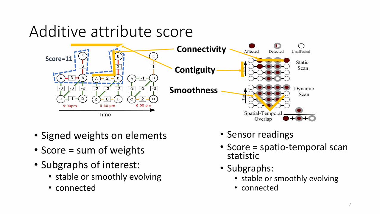
Additive attribute score

• Sensor readings• Score = spatio-temporal scan

statistic• Subgraphs:

• stable or smoothly evolving• connected

Score=11

• Signed weights on elements

• Score = sum of weights

• Subgraphs of interest:• stable or smoothly evolving• connected

7

Connectivity

Contiguity

Smoothness

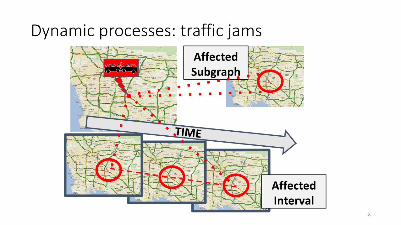
Dynamic processes: traffic jams

Affected Interval

Affected Subgraph

8

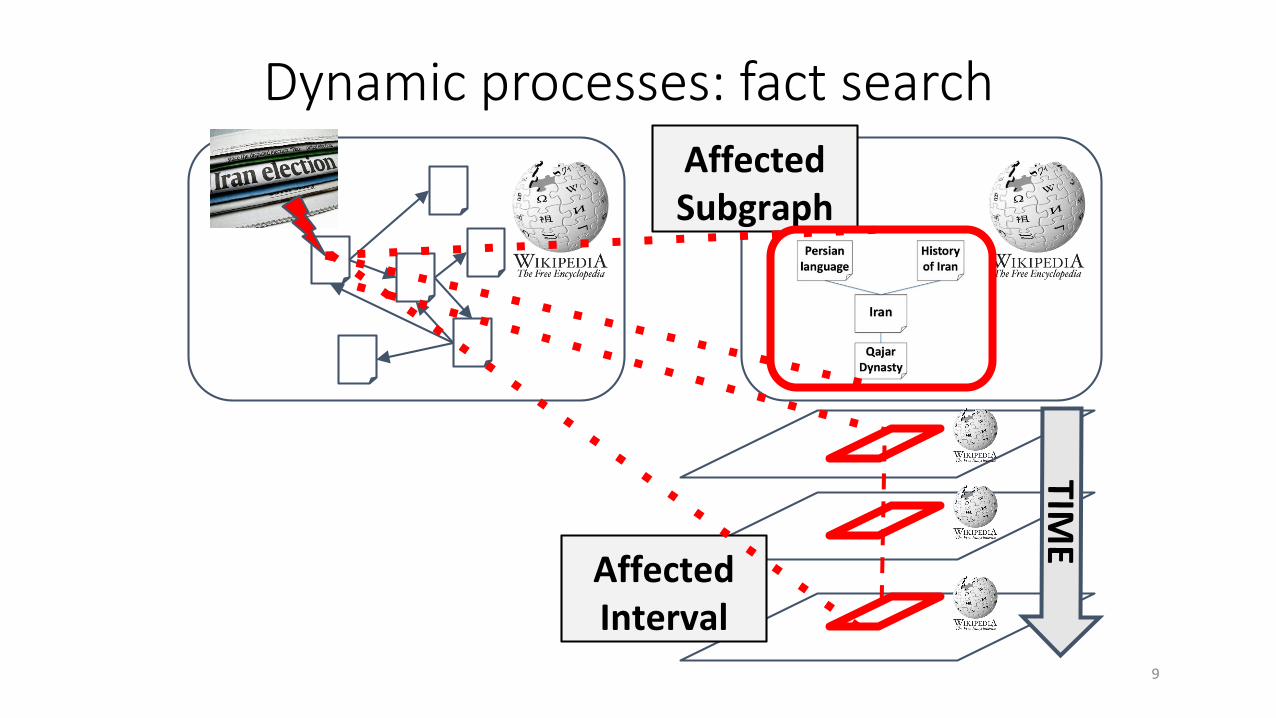
Affected Subgraph

Affected Interval

Dynamic processes: fact search

9

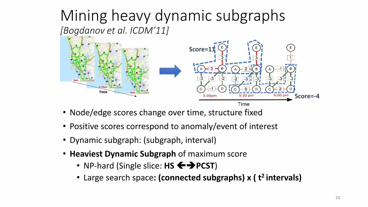
Mining heavy dynamic subgraphs[Bogdanov et al. ICDM’11]

• Node/edge scores change over time, structure fixed

• Positive scores correspond to anomaly/event of interest

• Dynamic subgraph: (subgraph, interval)

• Heaviest Dynamic Subgraph of maximum score

• NP-hard (Single slice: HS PCST)

• Large search space: (connected subgraphs) x ( t2 intervals)

Score=11

Score=-4

10

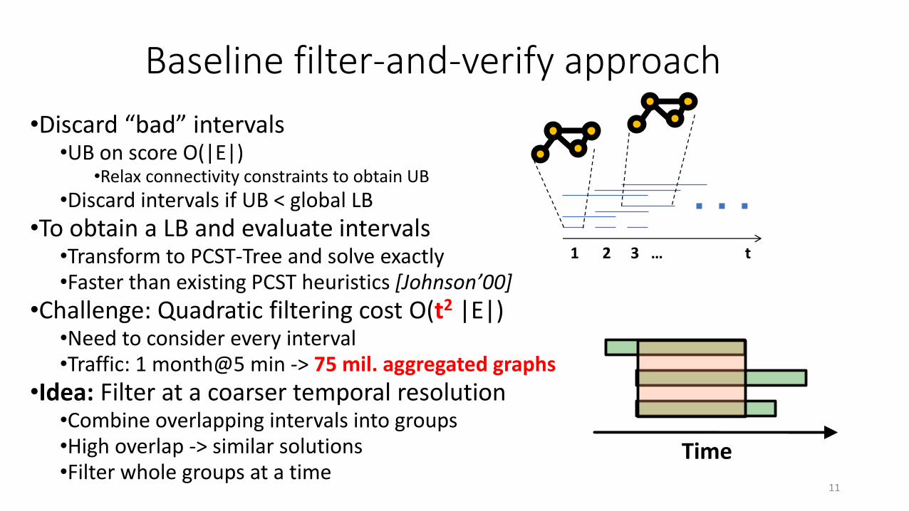
Baseline filter-and-verify approach

•Discard “bad” intervals•UB on score O(|E|)

•Relax connectivity constraints to obtain UB

•Discard intervals if UB < global LB

•To obtain a LB and evaluate intervals•Transform to PCST-Tree and solve exactly •Faster than existing PCST heuristics [Johnson’00]

•Challenge: Quadratic filtering cost O(t2 |E|)•Need to consider every interval•Traffic: 1 month@5 min -> 75 mil. aggregated graphs

•Idea: Filter at a coarser temporal resolution•Combine overlapping intervals into groups•High overlap -> similar solutions•Filter whole groups at a time

1 2 3 … t

Time

11

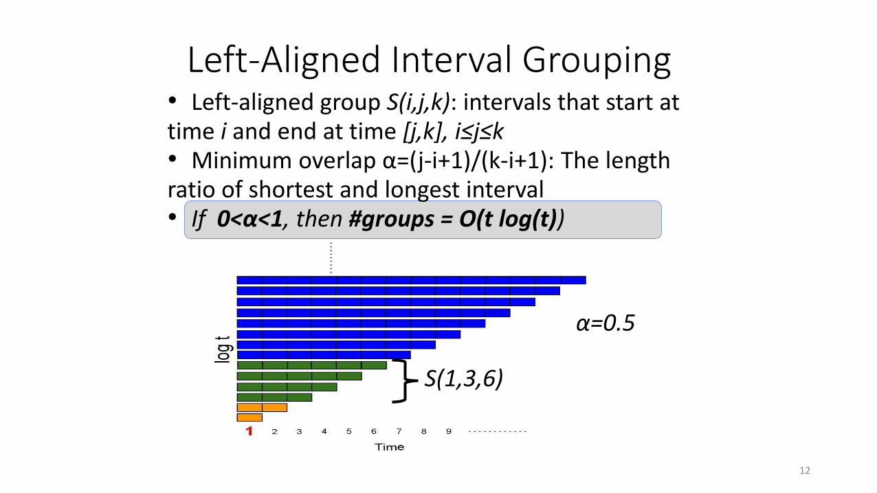
• Left-aligned group S(i,j,k): intervals that start at time i and end at time [j,k], i≤j≤k• Minimum overlap α=(j-i+1)/(k-i+1): The length ratio of shortest and longest interval • If 0<α<1, then #groups = O(t log(t))

Left-Aligned Interval Grouping

α=0.5

S(1,3,6)

12

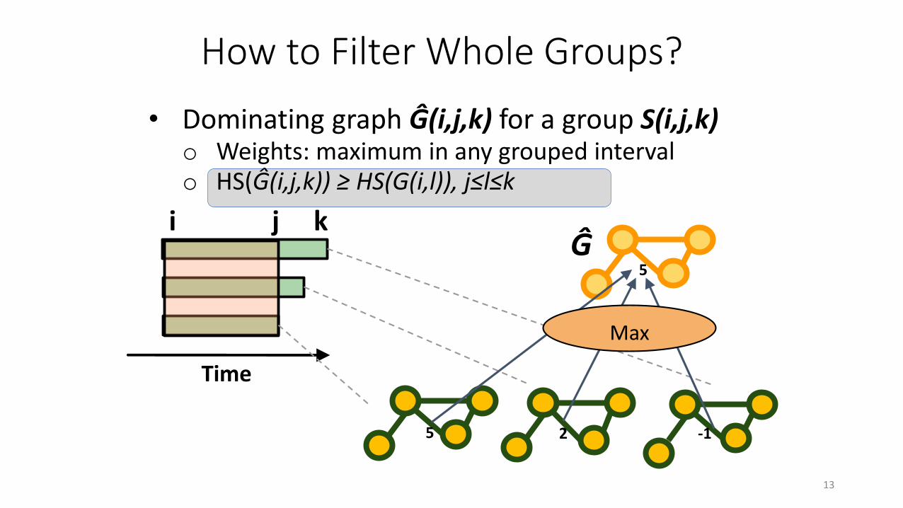
• Dominating graph Ĝ(i,j,k) for a group S(i,j,k)o Weights: maximum in any grouped intervalo HS(Ĝ(i,j,k)) ≥ HS(G(i,l)), j≤l≤k

Time

Max

Ĝ

How to Filter Whole Groups?

5 2 -1

5

i j k

13

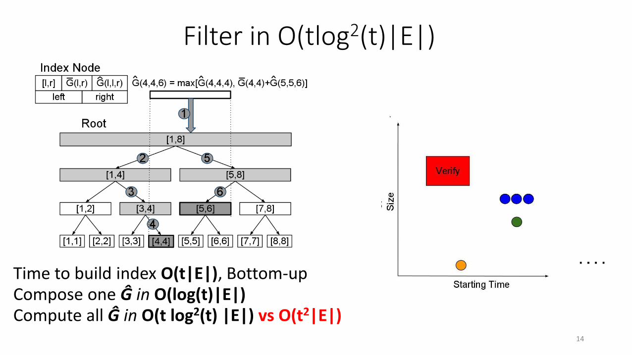
Time to build index O(t|E|), Bottom-upCompose one Ĝ in O(log(t)|E|)Compute all Ĝ in O(t log2(t) |E|) vs O(t2|E|)

Filter in O(tlog2(t)|E|)

14

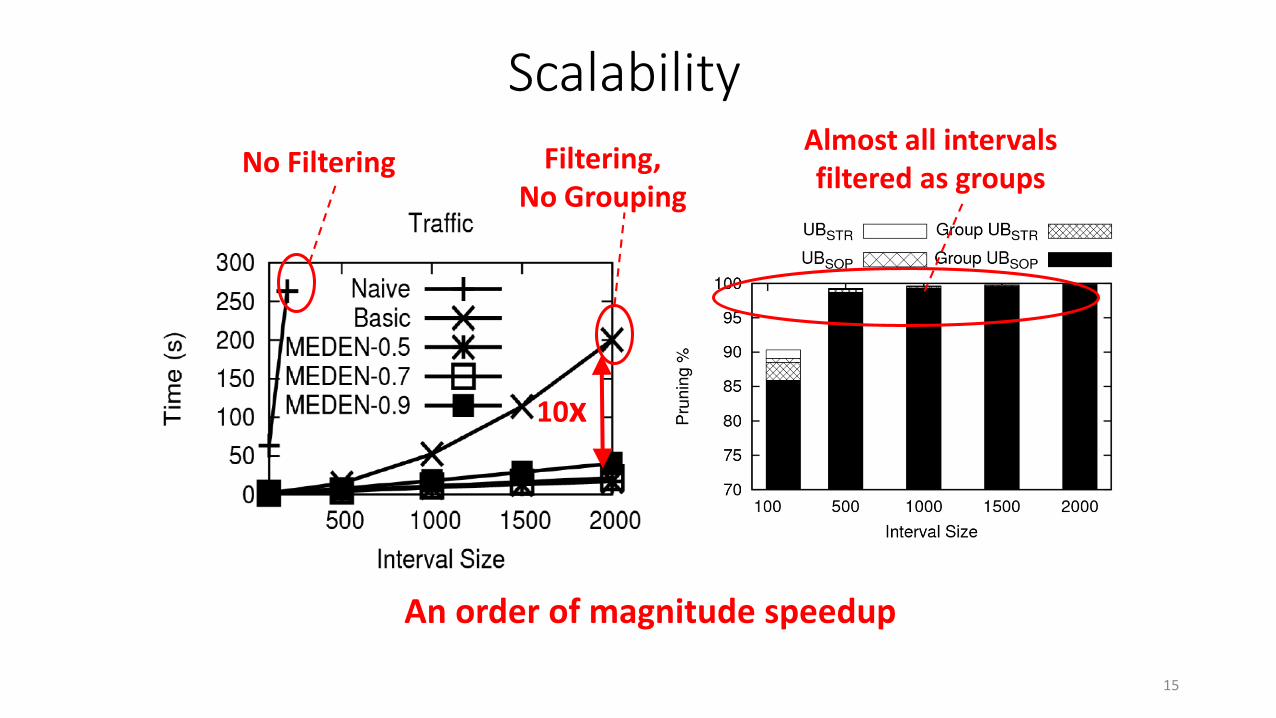
An order of magnitude speedup

10x

No FilteringAlmost all intervals filtered as groups

Scalability

Filtering, No Grouping

15

Identify All Significant Regions[Mongiovi et al. SDM’13]

• Alternate between optimization in the temporal and graph domains• Fix a subgraph: compute the MS time subsequence

• Fix a time interval: compute the Heaviest Subgraph

• Seeds: Heaviest subgraph, Max. Subsequence• Consider an augmented MST of every snapshot

• Optimal edge-rooted scores for every edge in O(|E|)

• Optimal edge-rooted interval

• Allow overlap

16

So far: “stable” solutions across time

• No change in participating nodes/edges

• Processes in real networks might shift and change in size

• Idea: incorporate smoothness• As a constraint: not too

many nodes/edges change• As a penalty

17

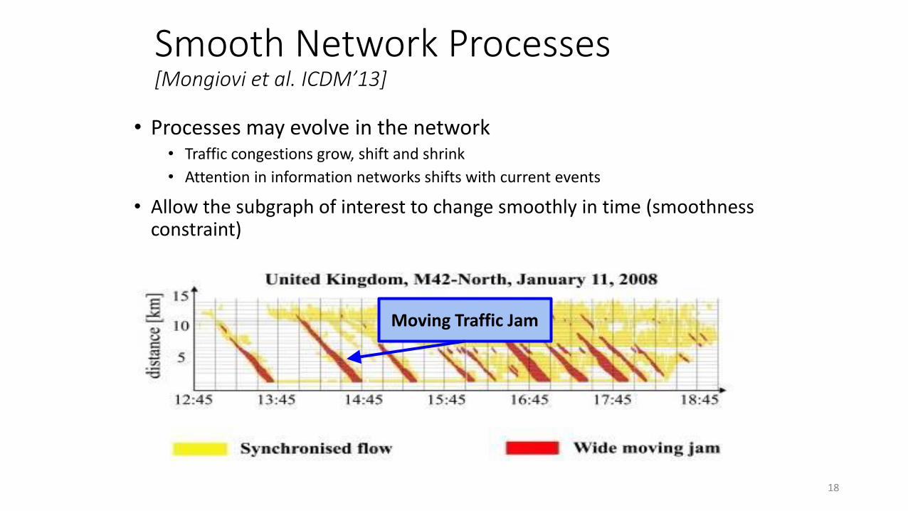
Smooth Network Processes [Mongiovi et al. ICDM’13]

• Processes may evolve in the network• Traffic congestions grow, shift and shrink

• Attention in information networks shifts with current events

• Allow the subgraph of interest to change smoothly in time (smoothness constraint)

Moving Traffic Jam

18

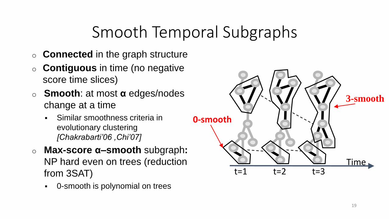
Smooth Temporal Subgraphso Connected in the graph structure

o Contiguous in time (no negative

score time slices)

o Smooth: at most α edges/nodes

change at a time

Similar smoothness criteria in

evolutionary clustering

[Chakrabarti’06 ,Chi’07]

o Max-score α–smooth subgraph:

NP hard even on trees (reduction

from 3SAT)

0-smooth is polynomial on trees

3-smooth

0-smooth

Timet=1 t=2 t=3

19

Overview of Solution

Accurate

Search

Dy

na

mic

N

etw

ork

No-loss

Filtering

LB Spot

SmoothUB

α-M

ineS

moo

th P

roce

ss

Reduce the instance size Candidate search

Timet=1 t=2 t=3

UB(v,t) < LBRemainingsmall and

fragmentedInstance

(~5% of original)

No Loss of Accuracy

Spot∞-smoothcandidates

“Smooth”each candidate according to α

20

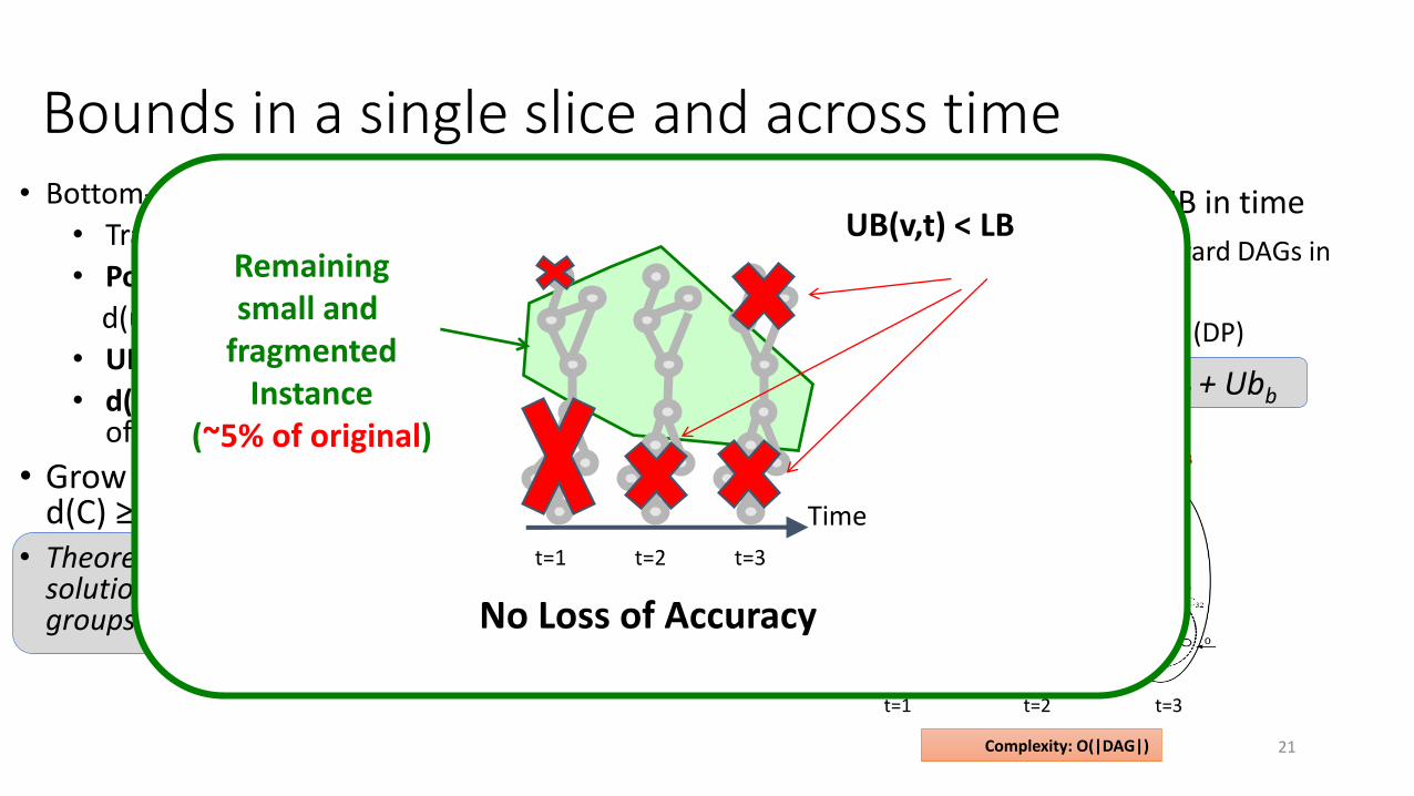
• Propagate single slice UB in time

• Construct forward/backward DAGs in time

• Propagate UB(t) on DAGs (DP)

• Theorem: UB= UBf + UBsl + Ubb

• Bottom-up node group bounding

• Transform to PCST

• Potential: p(u) = w(u) – d(u)/2,

d(u) = min (d(u,v)), w(v) >0

• UB(C) = max[Σp(u), max[w(u)]]

• d(C) = min[d(u)], u on border of C

• Grow groups until d(C) ≥ 2UB(C)

• Theorem: An optimal positive PCST solution cannot span isolated groups

Bounds in a single slice and across time

21

C3

C1

C2

d(C)≥2UB(C)

d(C)

isolated

5

4

0

1

05

22

136

2

d=10

p=0

t=1 t=2 t=3

Forward UBSlice UB

Backward UB

Complexity: O(|DAG|)

Time

t=1 t=2 t=3

UB(v,t) < LBRemainingsmall and

fragmentedInstance

(~5% of original)

No Loss of Accuracy

High-Quality Search: Spot&Smooth

Spot ∞-smoothcandidates

“Smooth”each candidate according to α

Best paths connecting positive components

t=2

remove

t=1

α=1

22

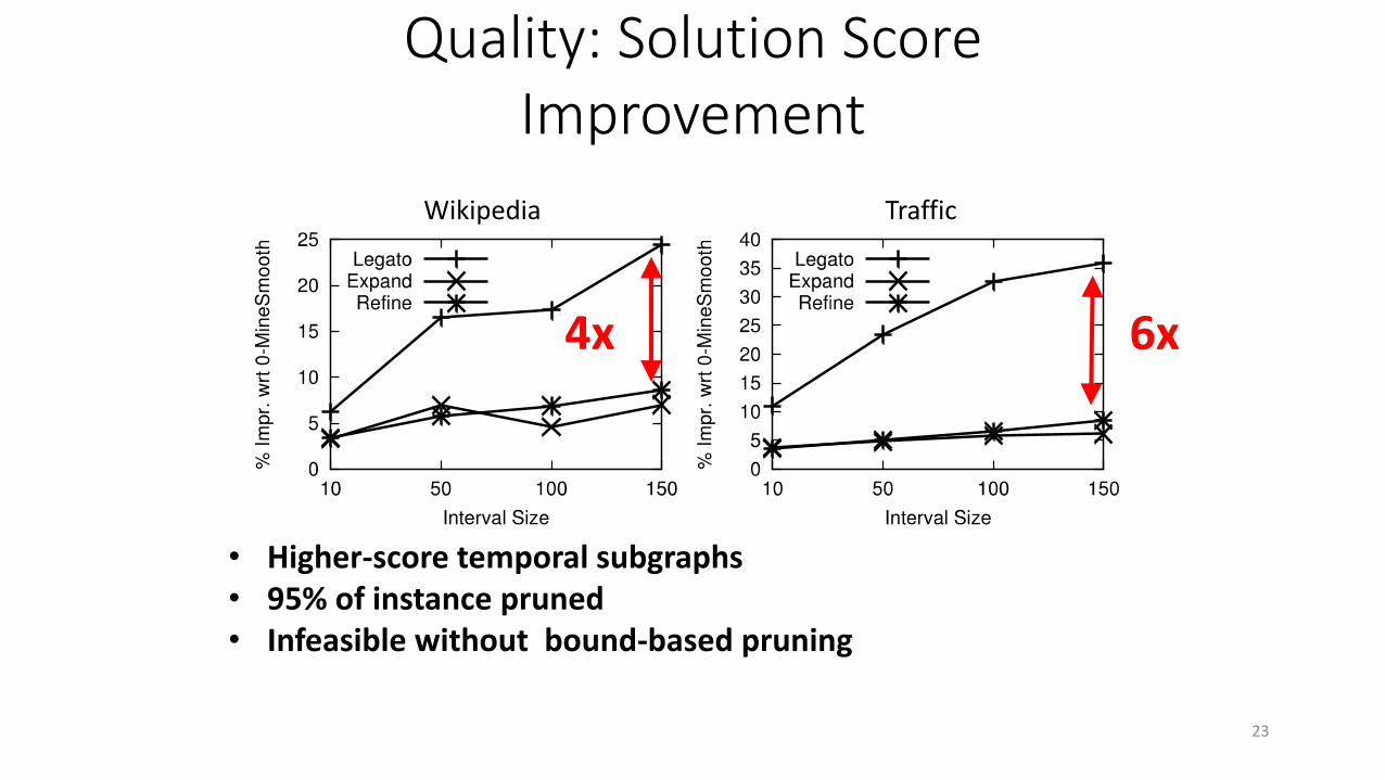
Quality: Solution Score Improvement

4x 6x

Wikipedia Traffic

• Higher-score temporal subgraphs• 95% of instance pruned• Infeasible without bound-based pruning

23

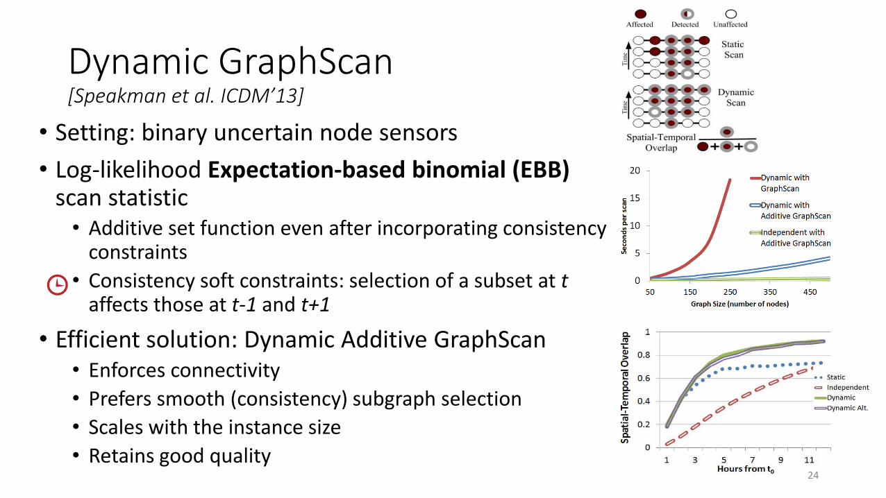
Dynamic GraphScan[Speakman et al. ICDM’13]

• Setting: binary uncertain node sensors

• Log-likelihood Expectation-based binomial (EBB) scan statistic• Additive set function even after incorporating consistency

constraints

• Consistency soft constraints: selection of a subset at taffects those at t-1 and t+1

• Efficient solution: Dynamic Additive GraphScan• Enforces connectivity

• Prefers smooth (consistency) subgraph selection

• Scales with the instance size

• Retains good quality24

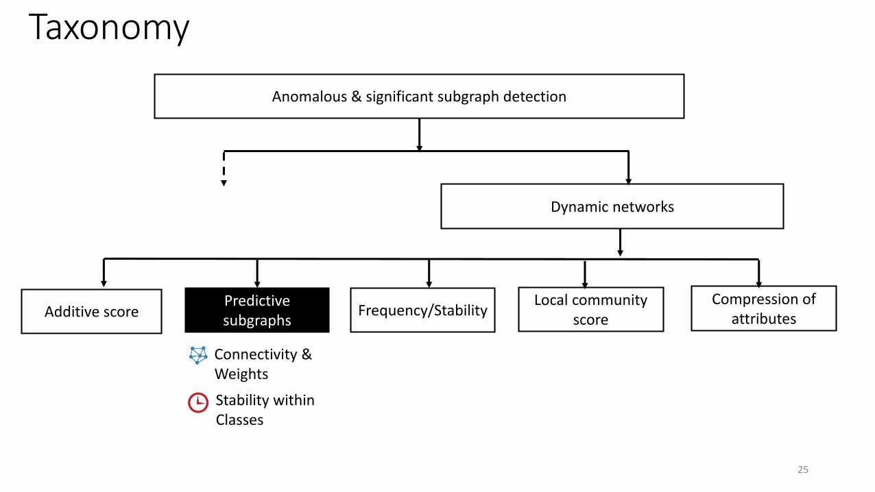
Taxonomy


Dynamic networks



score


25

Connectivity &Weights

Stability withinClasses

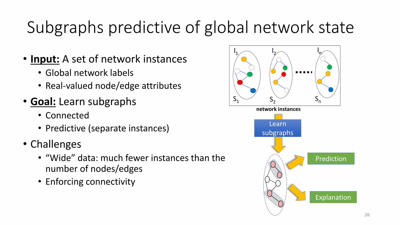
Subgraphs predictive of global network state

• Input: A set of network instances• Global network labels

• Real-valued node/edge attributes

• Goal: Learn subgraphs • Connected

• Predictive (separate instances)

• Challenges• “Wide” data: much fewer instances than the

number of nodes/edges

• Enforcing connectivity

network instances

S1 S2 Sn

l1 l2 ln

Prediction

Explanation

Learn subgraphs

26

MINDS: Network-constrained decision trees[Ranu et al. KDD’13]

• Idea: Learn decision trees based on node attributes, while ensuring connectivity

• Large search space: all connected subgraphs• MCMC sampling of trees

• Add nodes with probability proportional to their information gain (IG) increase

• Allow for removal of nodes

• Greedy DT construction in subgraph

• (+) Scalable and accurate• Compared to unconstrained SVM and Greedy

• (-) Sampling-based: non-deterministicUnconstrained Network-

constrained

27

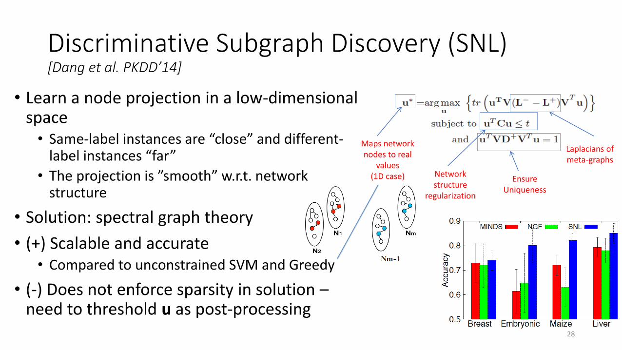
Discriminative Subgraph Discovery (SNL)[Dang et al. PKDD’14]

• Learn a node projection in a low-dimensional space• Same-label instances are “close” and different-

label instances “far”

• The projection is ”smooth” w.r.t. network structure

• Solution: spectral graph theory

• (+) Scalable and accurate• Compared to unconstrained SVM and Greedy

• (-) Does not enforce sparsity in solution –need to threshold u as post-processing

Maps network nodes to real

values (1D case)

Laplacians of meta-graphs

Network structure

regularization

Ensure Uniqueness

28

Prediction

Explanation

S

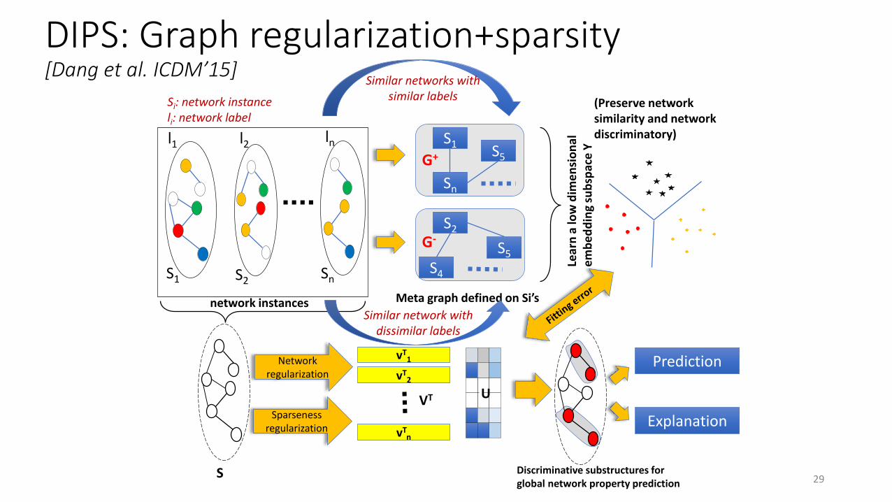
Network regularization

Sparsenessregularization

vT1

vT2

vTn

VT U

network instances

S1 S2Sn

l1 l2 ln

Similar networks with similar labels

Meta graph defined on Si’s

S1

Sn

S5G+

S2

S4

S5G-

Lear

n a

low

dim

en

sio

nal

e

mb

ed

din

g su

bsp

ace

Y

Discriminative substructures for global network property prediction

Similar network with dissimilar labels

Si: network instanceli: network label

(Preserve network similarity and network discriminatory)

DIPS: Graph regularization+sparsity[Dang et al. ICDM’15]

29

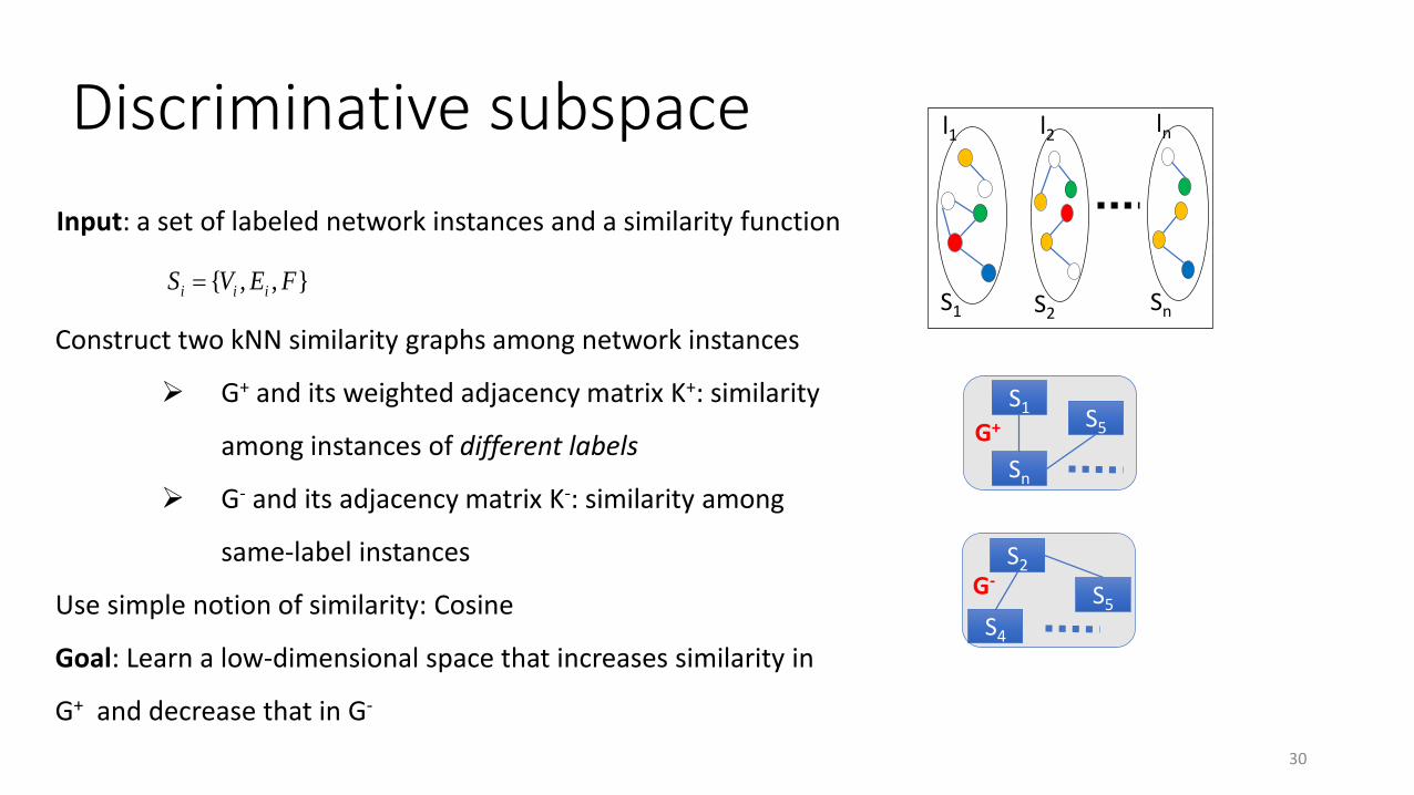
Construct two kNN similarity graphs among network instances

G+ and its weighted adjacency matrix K+: similarity

among instances of different labels

G- and its adjacency matrix K-: similarity among

same-label instances

Use simple notion of similarity: Cosine

Goal: Learn a low-dimensional space that increases similarity in

G+ and decrease that in G-

S1

Sn

S5G+

S2

S4

S5G-

Discriminative subspace

30

S1 S2 Sn

l1 l2 ln

Input: a set of labeled network instances and a similarity function

},,{ FEVS iii

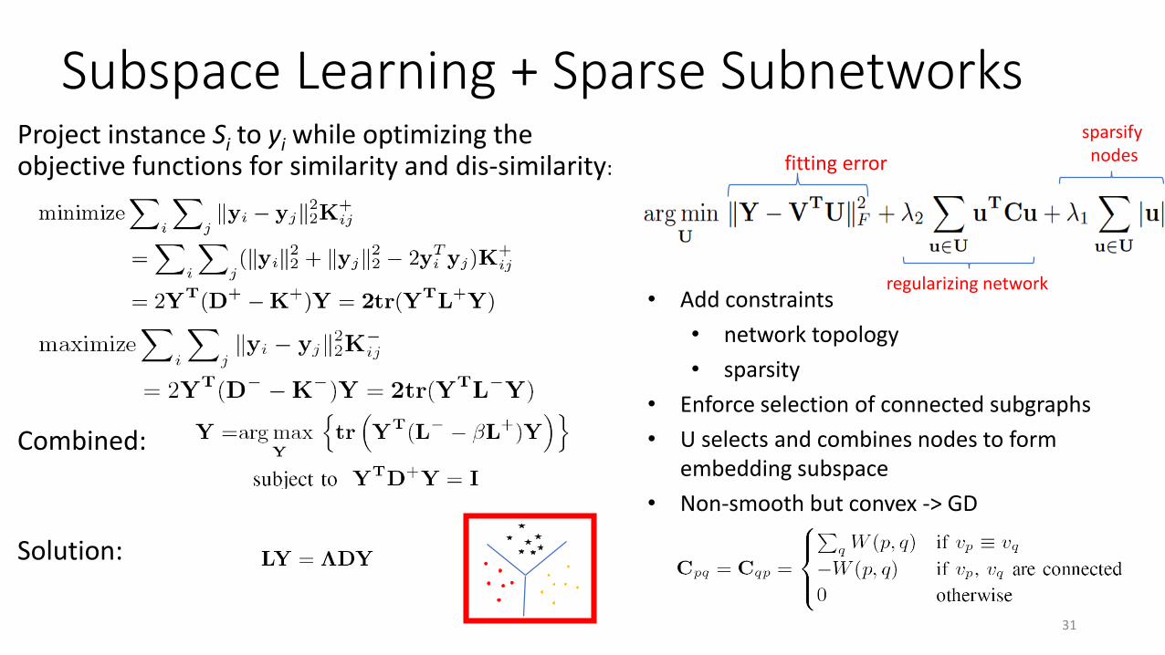
Project instance Si to yi while optimizing the objective functions for similarity and dis-similarity:

Combined:

Solution:

Subspace Learning + Sparse Subnetworks

31

sparsifynodes

regularizing network

fitting error

• Add constraints

• network topology

• sparsity

• Enforce selection of connected subgraphs

• U selects and combines nodes to form embedding subspace

• Non-smooth but convex -> GD

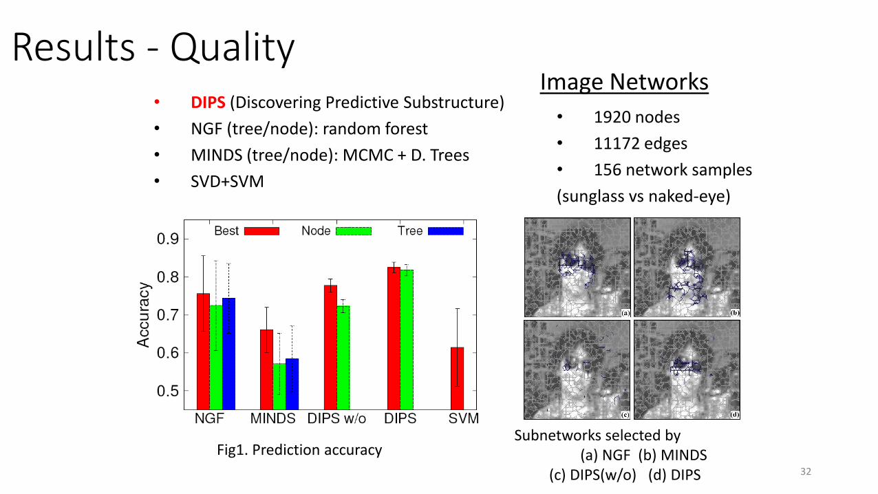
• 1920 nodes

• 11172 edges

• 156 network samples

(sunglass vs naked-eye)

Subnetworks selected by (a) NGF (b) MINDS

(c) DIPS(w/o) (d) DIPS

Fig1. Prediction accuracy

• DIPS (Discovering Predictive Substructure)

• NGF (tree/node): random forest

• MINDS (tree/node): MCMC + D. Trees

• SVD+SVM

Results - QualityImage Networks

32

• 2948 nodes (on average)

• 191750 edges


Predictive substructures largely reside in temporal lobe (TP.L, TP.R, T2a.R, T2p.L, T3a.R) and hippocampus (Hip.L/Hip.R),

Sparse SubnetworksBrain Networks

ground truth genes collected from literature

Gene Expression Networks

Embryonic development

• 1321 genes

• 5277 edges


Liver metastasis

• 7383 genes

• 251916 edges

• 123 network samples 33

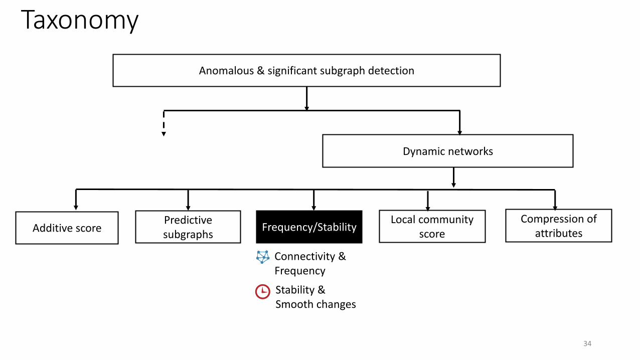
Taxonomy


Dynamic networks



score


34

Connectivity &Frequency

Stability & Smooth changes

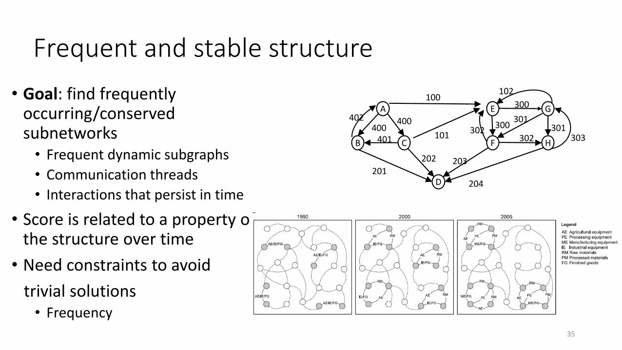
Frequent and stable structure

• Goal: find frequently occurring/conserved subnetworks• Frequent dynamic subgraphs

• Communication threads

• Interactions that persist in time

• Score is related to a property of the structure over time

• Need constraints to avoid

trivial solutions• Frequency

B

A

C

E

F

D

G

H

100

202

201203

102

101

204

300

300

302301400

401400

302301

303

402

35

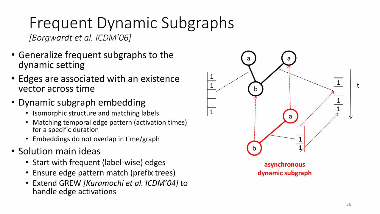
Frequent Dynamic Subgraphs[Borgwardt et al. ICDM’06]

• Generalize frequent subgraphs to the dynamic setting

• Edges are associated with an existence vector across time

• Dynamic subgraph embedding• Isomorphic structure and matching labels• Matching temporal edge pattern (activation times)

for a specific duration• Embeddings do not overlap in time/graph

• Solution main ideas• Start with frequent (label-wise) edges• Ensure edge pattern match (prefix trees)• Extend GREW [Kuramochi et al. ICDM’04] to

handle edge activations

36

a a

b

1

1

1

1

11

t

a

b

11

asynchronousdynamic subgraph

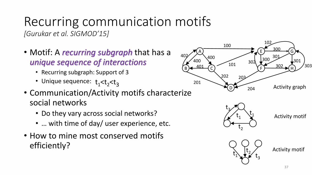
Recurring communication motifs[Gurukar et al. SIGMOD’15]

• Motif: A recurring subgraph that has a unique sequence of interactions• Recurring subgraph: Support of 3

• Unique sequence: 𝑡1 < 𝑡2 < 𝑡3

• Communication/Activity motifs characterize social networks• Do they vary across social networks?

• … with time of day/ user experience, etc.

• How to mine most conserved motifs efficiently?

B

A

C

E

F

D

G

H

100

202

201203

102

101

204

300

300

302301400

401400

302301

303

402

t1t1

t2

t3

Activity graph

Activity motif

t2t3

t1

Activity motif

37

t1<t2<t3

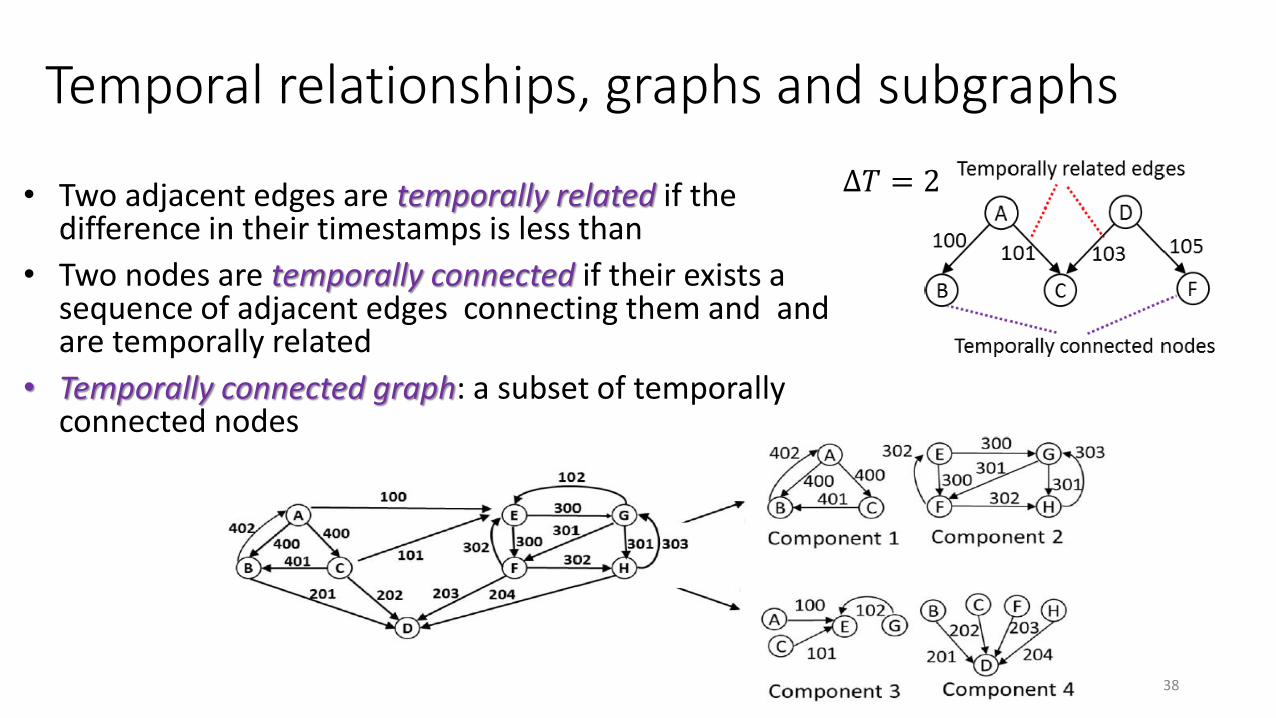
• Two adjacent edges are temporally related if the difference in their timestamps is less than

• Two nodes are temporally connected if their exists a sequence of adjacent edges connecting them and and are temporally related

• Temporally connected graph: a subset of temporally connected nodes

Temporal relationships, graphs and subgraphs

Δ𝑇 = 2

38

Temporally-isomorphic subgraphs

• Isomorphic subgraphs with the same sequence of information flow

B

A

C

400

401400

402E

F

G

300

300

300301

But, NOT temporally isomorphic:

Mine:All connected, temporally isomorphic subgraphs with support above 𝝉

• Problem: Given

3. Support threshold 𝜏

2. Temporal connectivity threshold Δ𝑇

1. Dynamic Interaction Network

B

A

C

E

F

D

G

H

100

202201

203

102

101

204

300

300

302301400

401400

302301

303

402

At 𝜏 = 3, Δ𝑇 = 1 39

COMMIT: Pipeline and main ideas

Replace node labels with degrees

Encode edges in sequence

Encoding sequences

Sequence growth

40

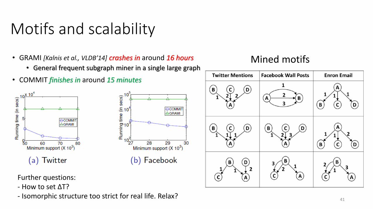
Motifs and scalability

Mined motifs• GRAMI [Kalnis et al., VLDB’14] crashes in around 16 hours

• General frequent subgraph miner in a single large graph

• COMMIT finishes in around 15 minutes

Further questions:- How to set ΔT?- Isomorphic structure too strict for real life. Relax?

41

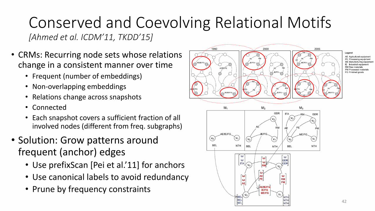
Conserved and Coevolving Relational Motifs[Ahmed et al. ICDM’11, TKDD’15]

• CRMs: Recurring node sets whose relations change in a consistent manner over time• Frequent (number of embeddings)

• Non-overlapping embeddings

• Relations change across snapshots

• Connected

• Each snapshot covers a sufficient fraction of all involved nodes (different from freq. subgraphs)

• Solution: Grow patterns around frequent (anchor) edges• Use prefixScan [Pei et al.’11] for anchors

• Use canonical labels to avoid redundancy

• Prune by frequency constraints42

Taxonomy


Dynamic networks


Additive scoreFrequency/(un)Sta

bilityLocal community

scoreCompression

43

Density &Quasi-cliques

(un) Stability & Recurrence &Span in time

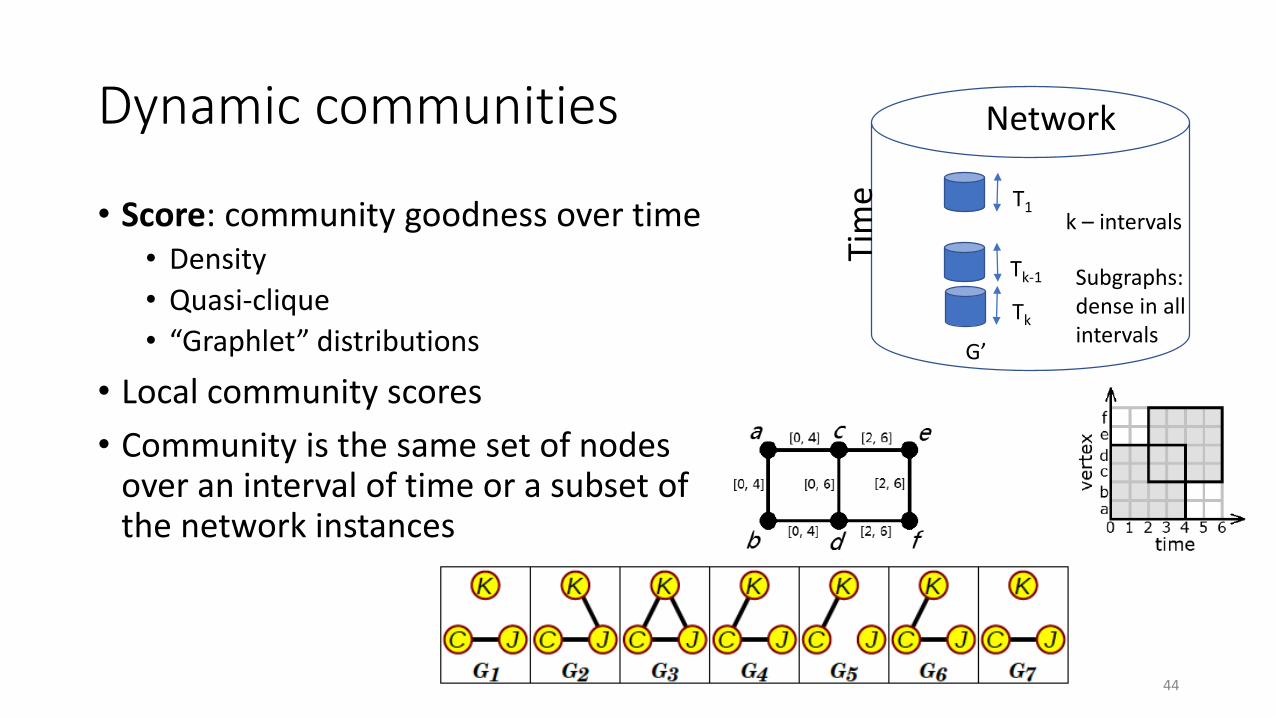
Dynamic communities

• Score: community goodness over time• Density

• Quasi-clique

• “Graphlet” distributions

• Local community scores

• Community is the same set of nodes over an interval of time or a subset of the network instances

Tim

e

Network

T1

Tk-1

Tk

G’

k – intervals

Subgraphs:dense in all intervals

44

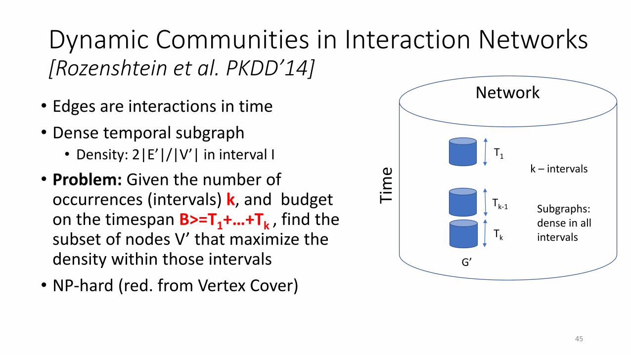
Dynamic Communities in Interaction Networks[Rozenshtein et al. PKDD’14]

• Edges are interactions in time

• Dense temporal subgraph• Density: 2|E’|/|V’| in interval I

• Problem: Given the number of occurrences (intervals) k, and budget on the timespan B>=T1+…+Tk , find the subset of nodes V’ that maximize the density within those intervals

• NP-hard (red. from Vertex Cover)

Tim

e

Network

T1

Tk-1

Tk

G’

k – intervals

Subgraphs:dense in all intervals

45

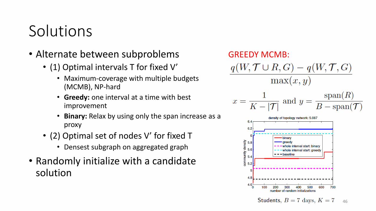
Solutions• Alternate between subproblems

• (1) Optimal intervals T for fixed V’• Maximum-coverage with multiple budgets

(MCMB), NP-hard

• Greedy: one interval at a time with best improvement

• Binary: Relax by using only the span increase as a proxy

• (2) Optimal set of nodes V’ for fixed T• Densest subgraph on aggregated graph

• Randomly initialize with a candidate solution

GREEDY MCMB:

46

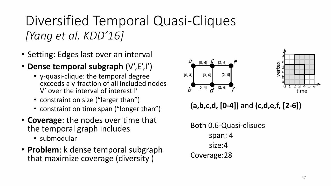
Diversified Temporal Quasi-Cliques[Yang et al. KDD’16]

• Setting: Edges last over an interval

• Dense temporal subgraph (V’,E’,I’)• y-quasi-clique: the temporal degree

exceeds a y-fraction of all included nodes V’ over the interval of interest I’

• constraint on size (“larger than”)• constraint on time span (“longer than”)

• Coverage: the nodes over time that the temporal graph includes• submodular

• Problem: k dense temporal subgraph that maximize coverage (diversity )

(a,b,c,d, [0-4]) and (c,d,e,f, [2-6])

Both 0.6-Quasi-clisuesspan: 4size:4

Coverage:28

47

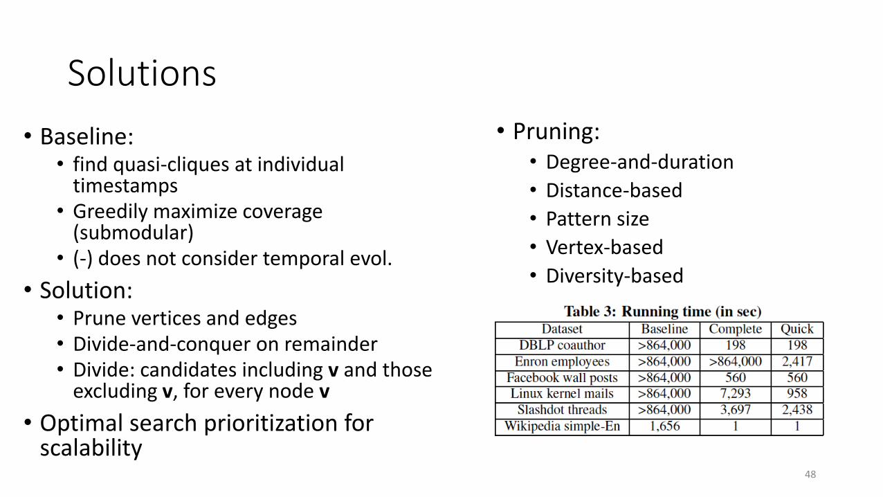
Solutions

• Baseline: • find quasi-cliques at individual

timestamps• Greedily maximize coverage

(submodular)• (-) does not consider temporal evol.

• Solution:• Prune vertices and edges• Divide-and-conquer on remainder• Divide: candidates including v and those

excluding v, for every node v

• Optimal search prioritization for scalability

• Pruning: • Degree-and-duration

• Distance-based

• Pattern size

• Vertex-based

• Diversity-based

48

Unstable Communities in Network Ensembles[Rahman et al. SDM’16]

• UC: Sets of nodes forming unstable ”configurations”

• Measure in terms of subgraph distributions

• Subgraph divergence: relative entropy of the observed subgraphs compared to uniform

• Problem: Find all maximal size-scaled subgraphs of divergence exceeding a threshold T• NP-hard• Anti-monotonicity -> Apriori-style

solution49

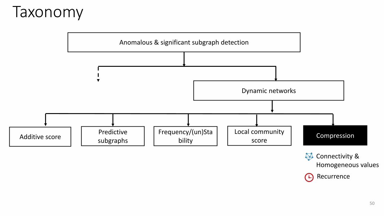
Taxonomy

50


Dynamic networks


Additive scoreFrequency/(un)Sta

bilityLocal community

scoreCompression

Connectivity &Homogeneous values

Recurrence

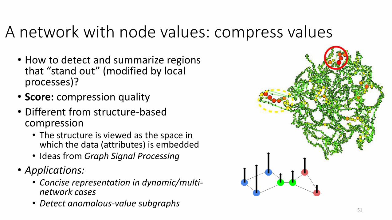
A network with node values: compress values

• How to detect and summarize regions that “stand out” (modified by local processes)?

• Score: compression quality

• Different from structure-based compression• The structure is viewed as the space in

which the data (attributes) is embedded• Ideas from Graph Signal Processing

• Applications: • Concise representation in dynamic/multi-

network cases• Detect anomalous-value subgraphs

51

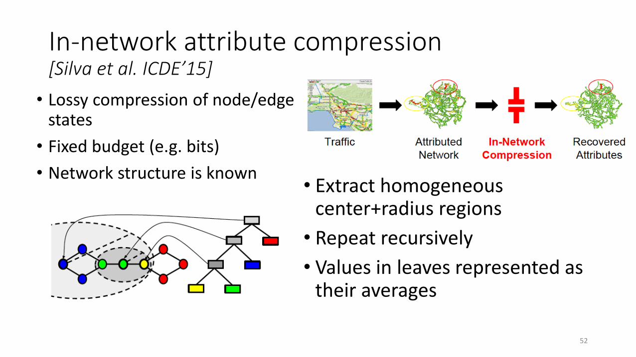
In-network attribute compression[Silva et al. ICDE’15]

• Lossy compression of node/edge states

• Fixed budget (e.g. bits)

• Network structure is known• Extract homogeneous

center+radius regions

• Repeat recursively

• Values in leaves represented as their averages

52

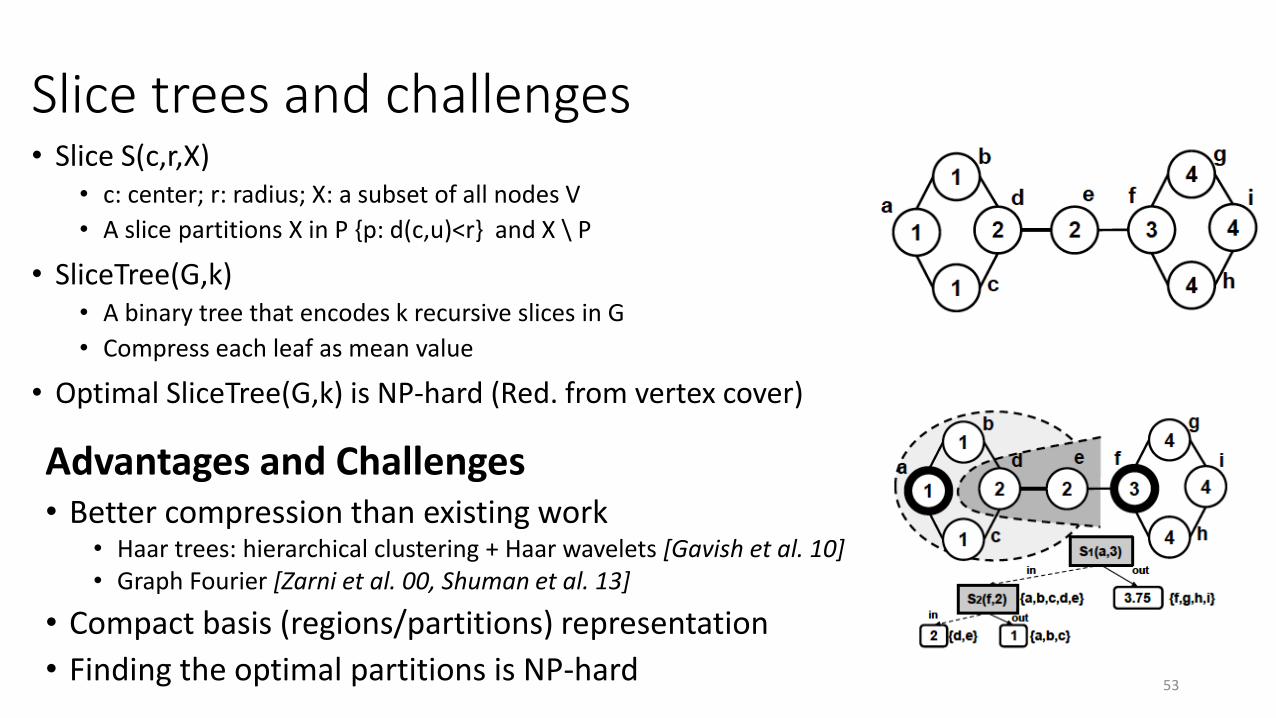
Slice trees and challenges• Slice S(c,r,X)

• c: center; r: radius; X: a subset of all nodes V

• A slice partitions X in P {p: d(c,u)<r} and X \ P

• SliceTree(G,k)• A binary tree that encodes k recursive slices in G

• Compress each leaf as mean value

• Optimal SliceTree(G,k) is NP-hard (Red. from vertex cover)

Advantages and Challenges• Better compression than existing work

• Haar trees: hierarchical clustering + Haar wavelets [Gavish et al. 10]• Graph Fourier [Zarni et al. 00, Shuman et al. 13]

• Compact basis (regions/partitions) representation

• Finding the optimal partitions is NP-hard53

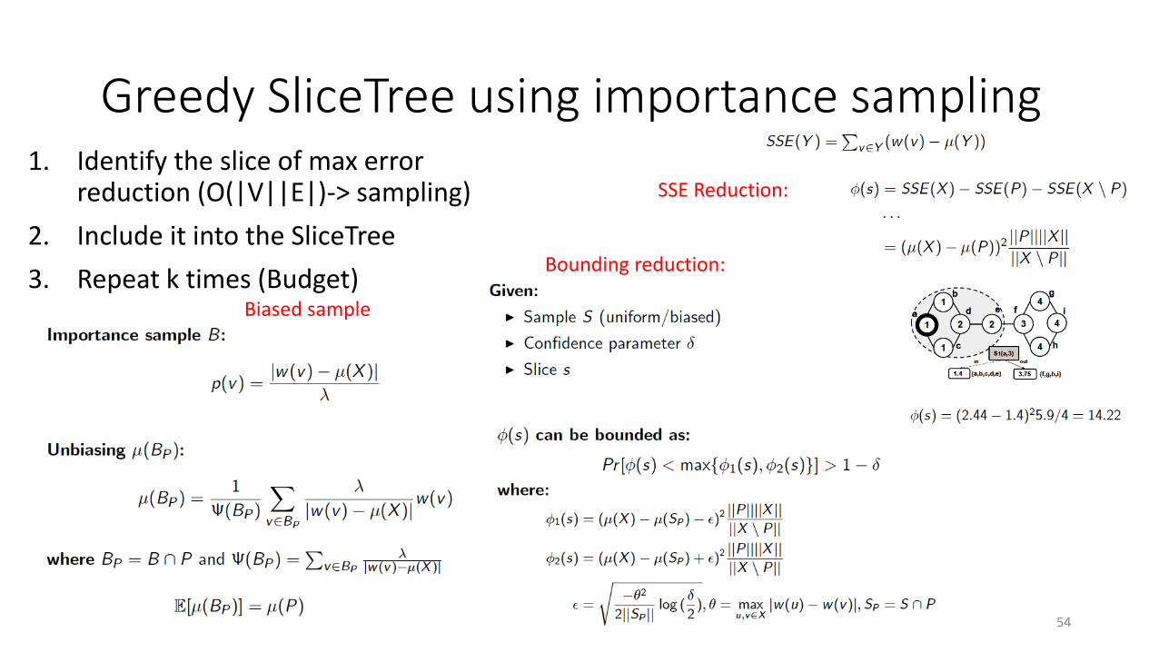
Greedy SliceTree using importance sampling1. Identify the slice of max error

reduction (O(|V||E|)-> sampling)

2. Include it into the SliceTree

3. Repeat k times (Budget)

SSE Reduction:

Biased sample

Bounding reduction:

54

Importance sampling

• 500x faster execution than naïve ST

• Small error + control over it

Traffic Gene expression

DBLP topics

• 80% reduction of SSE error with small number of bits (compared to full data)

• Exploits smoothness of attributes in the network

55

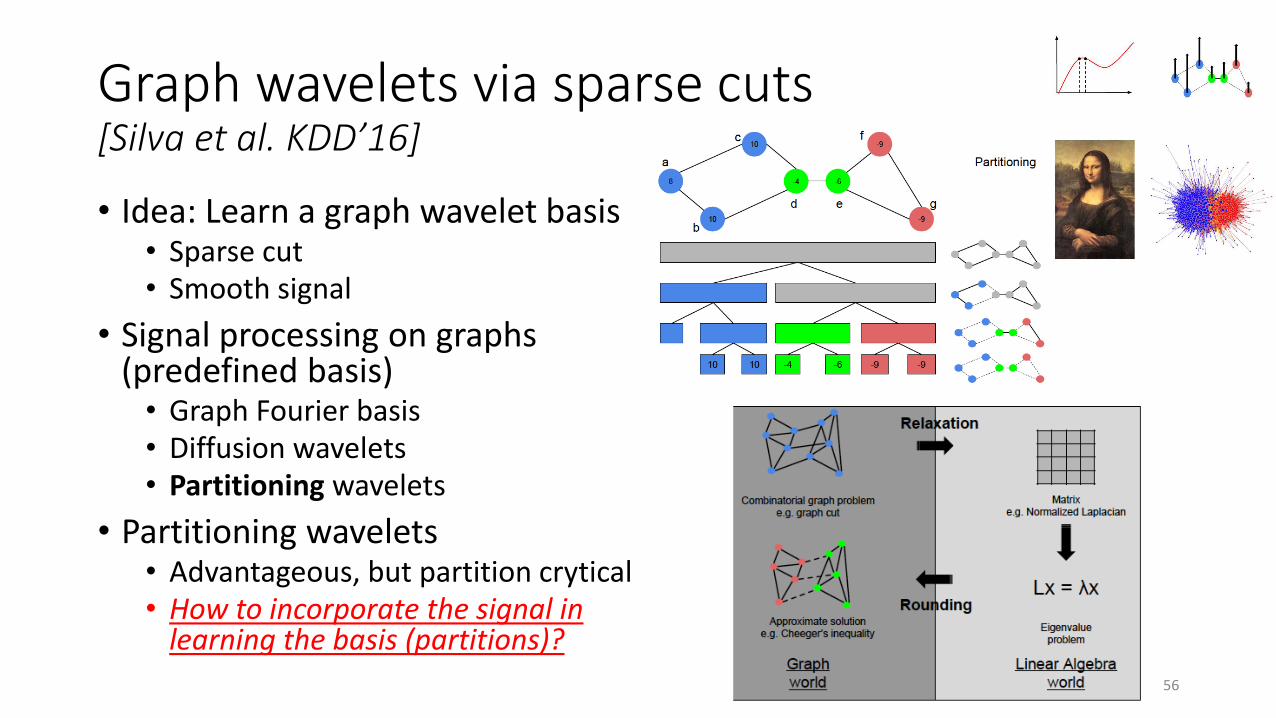
Graph wavelets via sparse cuts[Silva et al. KDD’16]

• Idea: Learn a graph wavelet basis• Sparse cut• Smooth signal

• Signal processing on graphs (predefined basis)• Graph Fourier basis• Diffusion wavelets• Partitioning wavelets

• Partitioning wavelets• Advantageous, but partition crytical• How to incorporate the signal in

learning the basis (partitions)?

56

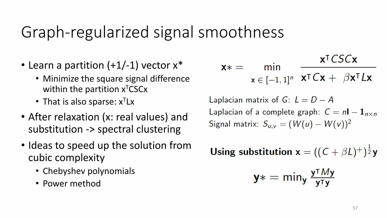
Graph-regularized signal smoothness

• Learn a partition (+1/-1) vector x*• Minimize the square signal difference

within the partition xTCSCx

• That is also sparse: xTLx

• After relaxation (x: real values) and substitution -> spectral clustering

• Ideas to speed up the solution from cubic complexity• Chebyshev polynomials

• Power method

57

Results

• 100x speed-up compared to exact, similar quality

• Superior performance to graph wavelet baselines

58

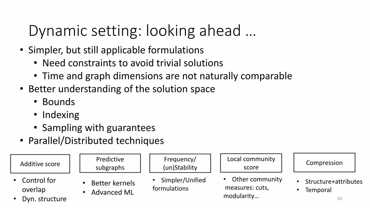
Dynamic setting: looking ahead …

59


Additive scoreFrequency/(un)Stability

Local community score

Compression

• Simpler, but still applicable formulations• Need constraints to avoid trivial solutions• Time and graph dimensions are not naturally comparable

• Better understanding of the solution space• Bounds• Indexing• Sampling with guarantees

• Parallel/Distributed techniques

• Control for overlap

• Dyn. structure

• Better kernels• Advanced ML

• Simpler/Unified formulations

• Other communitymeasures: cuts,

modularity…

• Structure+attributes• Temporal

Acknowledgements

• F. Chen would like to acknowledge support from NSF Grant IIS-1441479

• P. Bogdanov would like to acknowledge support from NSF Grant DMR-1309410 (Subaward: 75595)

• D. Neill would like to acknowledge support from NSF Grants IIS-0953330, NSF IIS-0916345, NSF IIS-0911032 and funding from the John D. and Catherine T. MacArthur Foundation

• A. Singh would like to acknowledge support from Army Research Lab NS-CTA W911NF-09-2-0053 and NSF Grant III-1219254

60

Part II: References• Rezwan Ahmed and George Karypis. Algorithms for mining the evolution of conserved relational

states in dynamic networks, ICDM, 2011

• Rezwan Ahmed and George Karypis, Algorithms for mining the coevolving relational motifs in dynamic networks, ACM Transactions on Knowledge Discovery from Data (TKDD), 2015

• Petko Bogdanov, Misael Mongiovi, and Ambuj K Singh, Mining heavy subgraphs in time-evolving networks. ICDM, 2011

• Xuan Hong Dang, Ambuj K Singh, Petko Bogdanov, Hongyuan You, and Bayyuan Hsu, Discriminative subnetworks with regularized spectral learning for global-state network data. PKDD, 2014.

• Xuan Hong Dang, Hongyuan You, Petko Bogdanov, and Ambuj K Singh. Learning predictive substructures with regularization for network data. ICDM, 2015

• Saket Gurukar, Sayan Ranu, and Balaraman Ravindran. Commit: A scalable approach to mining communication motifs from dynamic networks. SIGMOD, 2015.

• Misael Mongiovi, Petko Bogdanov, Razvan Ranca, Ambuj K Singh, Evangelos E Papalexakis, and Christos Faloutsos. Netspot: Spotting signicant anomalous regions on dynamic networks, SDM, 2013.

61

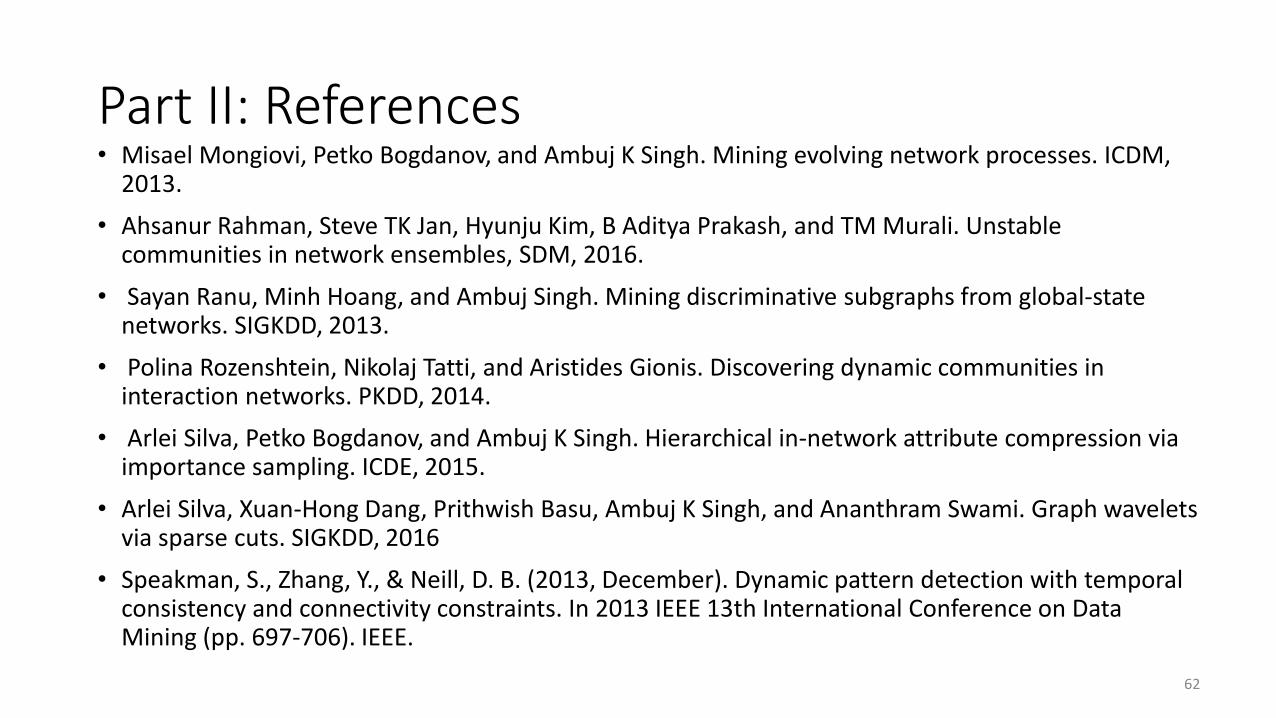
Part II: References• Misael Mongiovi, Petko Bogdanov, and Ambuj K Singh. Mining evolving network processes. ICDM,

2013.

• Ahsanur Rahman, Steve TK Jan, Hyunju Kim, B Aditya Prakash, and TM Murali. Unstable communities in network ensembles, SDM, 2016.

• Sayan Ranu, Minh Hoang, and Ambuj Singh. Mining discriminative subgraphs from global-state networks. SIGKDD, 2013.

• Polina Rozenshtein, Nikolaj Tatti, and Aristides Gionis. Discovering dynamic communities in interaction networks. PKDD, 2014.

• Arlei Silva, Petko Bogdanov, and Ambuj K Singh. Hierarchical in-network attribute compression via importance sampling. ICDE, 2015.

• Arlei Silva, Xuan-Hong Dang, Prithwish Basu, Ambuj K Singh, and Ananthram Swami. Graph wavelets via sparse cuts. SIGKDD, 2016

• Speakman, S., Zhang, Y., & Neill, D. B. (2013, December). Dynamic pattern detection with temporal consistency and connectivity constraints. In 2013 IEEE 13th International Conference on Data Mining (pp. 697-706). IEEE.

62

Thank you!

?Questions

63

Feng Chen

Petko Bogdanov

Daniel B. Neill

Ambuj K. Singh

anomalous and significant subgraph detection in attributed...

Documents