anomalous synchronization stability of power-grid network

Anomalous behavior of the synchronization stability on power-grid networks

Kim Heetae1, Lee Sang Hoon2, Son Seung-Woo3 Asia Pacific Center for Theoretical Physics

School of Physics, Korea Institute for Advanced Study Department of Applied Physics, Hanyang University

19 Oct. 2016 KPS 2016 Fall meeting, Kimdaejung Convention Center, Gwangju, South Korea

Anomalous behaviour of the synchronization stability on

power-grid networks





synchronization dynamics

i j

Power plant (P>0)

Power plant (P>0)

Consumer (P<0)

the phase angle of voltage at node i

i’s angular velocity (frequency)

adjacency matrix

the power input (P>0) or output (P<0)

the dissipation constant

the transmission capacity

θi ωi Aij Pi α K

!ω i = Pi −α !θi − K Aij sin(θi −θ j )∑!θi =ω i

Reference frameNode jNode i

G. Filatrella, A. H. Nielsen, and N. F. Pedersen, Eur. Phys. J. B 61, 485 (2008). P. J. Menck, J. Heitzig, N. Marwan, and J. Kurths, Nat Phys 9, 89 (2013).

Basin stability of a node ∈ [0,1]

Kumamoto-type model Synchronization [Basin] stability

The proportion of initial points among a given phase space, where the

oscillation results in synchrony.

Synchronization of power-grid

P. J. Menck, J. Heitzig, J. Kurths, and H. Joachim Schellnhuber, Nat Comms 5, 3969 (2014). P. Schultz, J. Heitzig, and J. Kurths, New J. Phys. 16, 125001 (2014). A. van Kan, J. Jegminat, J. F. Donges, and J. Kurths, Phys Rev E 93, 042205 (2016). P. Ji and J. Kurths, Eur. Phys. J. Spec. Top. 223, 2483 (2014).

<Northern European power grid>

creep into it, rattling and desynchronizing the nodes it contains.By this mechanism, multiple other sorts of non-synchronousstates can arise—for instance, the one depicted in Fig. 3d. Here alarge perturbation that initially affects node 6 (cf. Fig. 3a) leavesthis node almost synchronous but heavily desynchronizes thedead-end node 7 (which is pushed to oscillate around P7/a, cf.equation (3)).

These observations suggest that dead trees should drasticallylower the basin stability of nodes adjacent to them. We find thatthis is indeed the case (Fig. 3b). Furthermore, non-adjacent nodesdo display the increasing dependence of /SS on degree d we hadhypothesized earlier. It is now clear why we could not alreadyobserve this dependence in Fig. 2b: the characteristic shown thereis, basically, an average over the two curves of Fig. 3b. In thisaverage, the curve associated with nodes adjacent to dead treesbecomes ever more dominant as d increases because a randomlypicked node with large degree is very likely to be connected to atleast one stability-adverse dead tree. Conversely, as dead trees inour ensemble grids often consist of a single degree-one node, arandomly picked node whose neighbours have a large average

degree is unlikely to be connected to a dead tree. Hence, theincrease of the curves in Fig. 2c,d.

Case study. Do these results from the random-grid ensemblecarry over to real-world topologies? We now turn to a case studyof the Northern European power grid whose transmission part,with N¼ 236 nodes and E¼ 320 connections, is depicted in Fig. 4(see Methods and Supplementary Note 4). As before, in orderto concentrate on the effects of the wiring topology, we neglectother transmission and generation details, randomly assignN/2 net generators (with Pi¼ þ P) and N/2 net consumers(with Pi¼ #P) and perform numerical simulations of thecoarse-grained model equations (7 and 8) to estimate single-nodebasin stability Si for every node (see listing in SupplementaryTable 1). What we find is in line with the ensemble results: thegrid’s synchronous state is especially unstable against large per-turbations hitting nodes adjacent to or inside of dead ends ordead trees. For example, observe the poor basin stability values ofnodes 1, 2 and 3 indicated in Fig. 4.

Would a ‘healing’ of the appendices bring benefits? To checkthis, we virtually add transmission lines to the grid according to asimple procedure: for each dead tree, the node is identified inthe grid that has the minimum Euclidean distance to any nodeinside the tree, yet is not itself part of or adjacent to the tree.Then we add a transmission line between this node and the treenode it is so close to. These steps are repeated until all dead treeshave been ‘healed’. On the assumption that the costs for each newline are proportional to the Euclidean distance spanned, the totalcosts of the procedure depend on the order in which theappendices are handled. We employ the most cost-efficient order.

This leaves us with 27 extra lines, of which some are shown inred in the insets of Fig. 4 (all of them are shown in SupplementaryFig. 2). Admittedly, this is a quick fix, and some of these lines maybe impossible to build in the real world because of geologicalconstraints such as mountain ridges. Nevertheless, it is illustrativeto evaluate the impact of the new topology they induce.

Therefore, we now re-estimate the single-node basin stabilityfor all nodes. The results, listed in Supplementary Table 1 andillustrated in the insets of Fig. 4, demonstrate that these few extralines—just 8% of the total number—suffice to improve stabilitysignificantly. In particular, the amended grid has no poor-stability(red) nodes anymore.

DiscussionWe have investigated the stability of power grids by means of acomponent-wise version of basin stability, a method that has notbeen used before and, we believe, might also benefit investigationsinto other multicomponent systems, including ecosystems25, foodwebs26 and gene regulatory networks27,28. Specifically, we haveassigned to each node of a power grid a number called single-node basin stability that measures how stable the grid’ssynchronous state is against large perturbations hitting thatnode. This way, nodes can roughly be classified into three groups,corresponding to poor stability, fair stability and high stability.

Of the many functional aspects that presumably matter for thisstability classification, we have focussed on the impact of thenetwork topology and performed a statistical analysis of anensemble of artificially generated power grids. We have foundseveral clear relationships: first, as one might expect, nodes thathave a large degree and are thus strongly coupled to the grid arelikely to have high stability. Second, and less expected, nodesadjacent to dead ends or dead trees are likely to possess poorstability, and on average even show much poorer stability thannodes that terminate such appendices. In a detailed investigationof the grid dynamics, we uncovered that this is because of the fact

3

2 146

7

5

Increasing S

Generator

0

0

P!

Consumer

Non-adjacent⟨S

⟩Adjacent

d

"1"2"3"4

Time

Time

"4"6"7

2 3 4 5 6 7 8

1

0.75

0.50

0.25

0

""

P!–

–

Figure 3 | Effects of dead ends and dead trees. (a) Shown is a snippetfrom the Northern European power grid (see Fig. 4). Squares (circles)depict net consumers with Pi¼ # P (net generators with Pi¼ þ P). Thecolour scale indicates how large a node’s basin stability Si is. The set ofnodes {4, 5, 6, 7} makes up a dead tree that includes two dead ends: {5}and {6, 7}. Nodes 4 and 6 have the distinct betweenness valuesb4¼ 3N# 10 and b6¼N# 2. As expected from Fig. 3e,f, they possess apoor basin stability. Note that the nodes labelled {1, 2, 3, 4, 5, 6, 7} herecorrespond to nodes {91, 90, 85, 88, 89, 87, 86} in Supplementary Table 1and Supplementary Note 4. (b) Ensemble average basin stability /SS ofnodes of degree d that are adjacent or non-adjacent to dead trees. Shadesindicate±one s.d. Nodes inside dead trees are not included in the statistics.(c,d) Time series of nodal frequencies after a particular perturbation has hitnode (c) 2, (d) 6 of the network snippet shown in (a). Ensemble simulationparameters: N¼ 100, E¼ 135, a¼0.1, P¼ 1 and K¼8 (see Methods).

NATURE COMMUNICATIONS | DOI: 10.1038/ncomms4969 ARTICLE

NATURE COMMUNICATIONS | 5:3969 | DOI: 10.1038/ncomms4969 | www.nature.com/naturecommunications 5

& 2014 Macmillan Publishers Limited. All rights reserved.

that dead trees provide easy access to certain non-synchronousstates in state space. In addition, the effect is a strong one: a nodeadjacent to a dead tree is likely to have poor stability even if it hasa large degree.

In a case study of the Northern European power grid, we haveobserved that nodes adjacent to dead trees indeed tend to havepoor stability and established that the inverse statement is alsotrue: ‘healing’ of dead trees through addition of transmission linessubstantially enhances stability.

When interpreting these findings, one has to take into accountthe simplifications our study is based on. First, we have sought toobtain a maximally clear view on the effects that the topology hason grid stability, and for that purpose neglected a host of otherdetails on generators, load characteristics and transmissionsystems. Second, we have treated large perturbations as initiallyaffecting only two of our model grids’ 2N-dimensions, disregard-ing that any real short circuit, load switching or severe fluctuationin renewable generation is sure to affect every node in a grid tosome extent.

On one hand, these simplifications should gradually beovercome in future studies by incorporating ever more dynamicaldetails and inhomogeneities, and by striving for more realistic,higher dimensional representations of large perturbations. As afirst step beyond the single-node perspective offered here, onecould for instance investigate how actual short circuits may affectlocalized groups of nodes. On the other hand, the simplificationshave enabled us to isolate a drastic effect of the topology on thedynamics: the mere presence of dead trees makes it easier to push

a grid into a blackout-inducing non-synchronous state. As themodel we use captures the complex nonlinear coupled-rotating-mass dynamics that is among the main determinants of a powergrid’s response to large perturbations, we consider it likely thatthis effect also exists in the real world.

There may be different remedies to the adverse impact ofdead trees. Congruent with the focus of this study, we havesuggested a topological solution: ‘healing’ of dead trees throughaddition of transmission lines. Other solutions on which researchcould be performed may include increasing the transfer capacityof lines inside a dead tree or placing extra control devices ordamper windings at particular nodes. The point is that dead treesappear to make such additional investment necessary—or elseincrease the risk of a potentially very expensive29–31 large-scaleblackout. Therefore, we propose to add one item to the list ofpower grid design principles: in order not to topologicallyundermine grid stability, avoid dead ends! With regard to theworldwide effort of making power grids more sustainable byconnecting new low-carbon generation facilities, it might beparticularly worth heeding this principle: when taking intoaccount systemic risks and burdens, the seemlingly cheapestconnection schemes, tree-like structures, may not be so cheapafter all.

What remains to be done? A very concrete question arises fromthe ‘healing’ procedure we have applied to the NorthernEuropean grid: whereas the addition of transmission linessignificantly benefitted the single-node basin stability of 30 ofthe 236 nodes (see Supplementary Table 1), at the same time it

1

I

2

Finland

Sweden

Norway

Denmark II

III

3

4

Increasing S

ConsumerGenerator

Figure 4 | Northern European power grid. The grid has N¼ 236 nodes and E¼ 320 transmission lines. The load scenario was chosen randomly, withsquares (circles) depicting N/2 net consumers with Pi¼ " P (net generators with Pi¼ þ P). The colour scale indicates how large a node’s basin stability Si

is. Insets I–III show that re-computed basin stability values after 27 lines have been added in order to ‘heal’ dead trees. New lines are coloured red. Oursimulation parameters, a¼0.1, P¼ 1 and K¼ 8, imply the simplifying assumptions that all generators in the grid are of the same making and that alltransmission lines are of the same voltage and impedance. These assumptions enable us to focus on the effects of the (unweighted) topology. For details,see Methods, Supplementary Table 1 and Supplementary Note 4. Note that the nodes labelled {1, 2, 3, 4} here correspond to nodes {192, 208, 96, 176} inthe listings in the Supplementary Information.

ARTICLE NATURE COMMUNICATIONS | DOI: 10.1038/ncomms4969

6 NATURE COMMUNICATIONS | 5:3969 | DOI: 10.1038/ncomms4969 | www.nature.com/naturecommunications

& 2014 Macmillan Publishers Limited. All rights reserved.

Previous study

1

0

Community consistency

1

0

∆K/∆Kmax

Φ: community consistencyk: degreeC: clustering coefficientF: current flow betweenness centrality.

Figure 5.ΔK and community consistency. This is basically a scatter plot but the darker points representmore points, drawnwithtransparency.

Table 1.Pearson correlation coefficient r ofΔK versuscommunity consistency (Φ), degree (k), clustering coeffi-cient (C), and current flowbetweenness (F) centrality.

Φ k C F

r −0.581 0.033 −0.054 0.072p-value < 10−3 0.500 0.266 0.139

Figure 6.ΔK /ΔKmax (left panel) and community consistency (right panel) of theChilean power grid, withΔKmax is themaximumΔK value among the nodes. The insets show the area of interest with the nodeswith largeΔK and small community consistency.

7

New J. Phys. 17 (2015) 113005 HKim et al

Stability transition

Node 7 Node 4 Node 8 Node 9 Node 12

Node 16Node 2 Node 3 Node 10 Node 11

Node 17Node 1

Node 18

0

1

0 25

Bas

inst

abil

ity

K

Node 6 Node 5 Node 14 Node 13

Node 15

<Synchronization stability analysis on a toy model>

H. Kim, S. H. Lee, and P. Holme, New J. Phys. 17, 113005 (2015). H. Kim, S. H. Lee, and P. Holme, Phys Rev E 93, 062318 (2016).

Consumer

Producer




Node 17Node 1

Node 18

0

1

0 25

Bas

inst

abil

ity

K


Node 15





Node 17Node 1

Node 18

0

1

0 25

Bas

inst

abil

ity

K


Node 15



Node 17Node 1

Node 18

0

1

0 25

Bas

inst

abil

ity

K


Node 15



Node 17Node 1

Node 18

0

1

0 25

Bas

inst

abil

ity

K


Node 15



Node 17Node 1

Node 18

0

1

0 25

Bas

inst

abil

ity

K


Node 15



�

��

��

��

��

�

� ��

0

1

0 20 40

B

K

Producer

Consumer

1300

400

H. Kim, S. H. Lee, and P. Holme, Phys Rev E 93, 062318 (2016).

Legend

Phase diagram of dynamics

e5n1k14

-π -π/2 0 π/2 π-100

-50

0

50

100

ωe5n1k7

-π -π/2 0 π/2 π-100

-50

0

50

100

ω

e5n1k21

-π -π/2 0 π/2 π-100

-50

0

50

100

ω

e5n1k28

-π -π/2 0 π/2 π-100

-50

0

50

100

ω

�

��

��

��

��

�

� ��

K=7.0 K=14.0 K=28.0K=21.0

Achieve sync

Fail to sync

ω

K

B

Phase diagram of dynamics

e5n1k14

-π -π/2 0 π/2 π-100

-50

0

50

100

ω

e5n1k125

-π -π/2 0 π/2 π-100

-50

0

50

100

ω

e5n1k7

-π -π/2 0 π/2 π-100

-50

0

50

100

ω

e5n1k15

-π -π/2 0 π/2 π-100

-50

0

50

100ω

e5n1k17

-π -π/2 0 π/2 π-100

-50

0

50

100

ω

e5n1k21

-π -π/2 0 π/2 π-100

-50

0

50

100

ω

e5n1k28

-π -π/2 0 π/2 π-100

-50

0

50

100

ω

�

��

��

��

��

�

� ��

K=7.0 K=14.0 K=28.0

K=12.5 K=15.0 K=17.0

K=21.0

Achieve sync

Fail to sync

ω

e5n1k13

-π -π/2 0 π/2 π-100

-50

0

50

100

ω

K=13.0

K

B

Oscillation trajectory

K=15 K=17 K=18 K=28K=16

-13

0

13

495 500

ω

Time(s)-13

0

13

495 500

ω

Time(s)-13

0

13

495 500

ω

Time(s)

-13

0

13

495 500

ω

Time(s)-13

0

13

495 500

ω

Time(s)-13

0

13

495 500

ω

Time(s)-13

0

13

495 500

ω

Time(s)-13

0

13

495 500

ω

Time(s)

-13

0

13

495 500

ω

Time(s)

K=7 K=12K=11K=10

�

��

��

��

��

�

� �� K

Bω1=17 θ1=0 ω2,3,4=0 θ2,3,4=0

Anomalous behaviour of the synchronization stability on

power-grid networks





Chilean power-grid network

• 420 Nodes ↳129 power plants

291 substations • 543 Links

• 1252 Nodes ↳285 power plants

967 substations • 961 Links

Chilean power-grid network

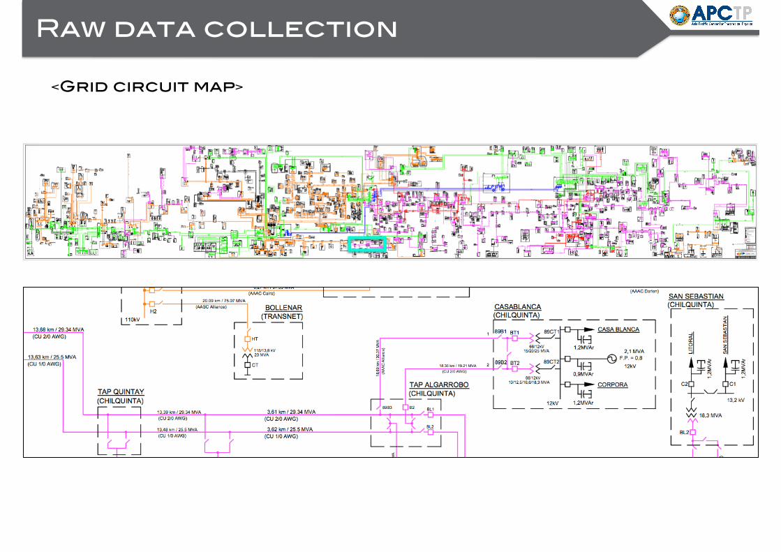
Raw data collection

<Activity data with time series>

Aggregated activity

t=1t=2

…

Raw data collection

<Field trip>

Raw data collection

<Grid circuit map>

San Andres Robleria

Rapel Pangue

Total Chilean power grid

Various patterns

Campiche Candelaria

RecaRio Tureno

Eolica Los Cururos Eolica Punta Palmeras

Solar Llano Llampos Solar Santa Cecilia

The Various Duration of Activity

The Pattern of Hydro Power

The Pattern of Wind Power

The Pattern of Solar Power

Conclusions

Stability analysis: Second order Kuramoto-type model Meso-scale: community characteristics ✓ Micro-scale: motif study ✓

Observed: Anomalous peak in stability transition

Data: Chilean power-grid network with richer information

Theoretical side

Application side

Acknowledgement

Prof. Claudio TenreiroProf. Eduardo Álvarez-Miranda David Olave Rojas

Acknowledgement

Thank you for your attention

sincerely appreciate your being my neighbour node.

and

anomalous synchronization stability of power-grid network

Science