anomaly detection in machine-generated data: a …621699/fulltext01.pdf · anomaly detection is an...

Anomaly Detection in

Machine-Generated Data: A Structured Approach

A N D R É E R I K S S O N

Master of Science Thesis Stockholm, Sweden 2013

Anomaly Detection in

Machine-Generated Data: A Structured Approach

A N D R É E R I K S S O N

Master’s Thesis in Mathematical Statistics (30 ECTS credits) Master Programme in Computer Science (120 credits) Royal Institute of Technology year 2013 Supervisor at KTH was Timo Koski Examiner was Timo Koski

TRITA-MAT-E 2013:14 ISRN-KTH/MAT/E--13/14--SE Royal Institute of Technology School of Engineering Sciences KTH SCI SE-100 44 Stockholm, Sweden URL: www.kth.se/sci

Abstract

Anomaly detection is an important issue in data mining and analysis, with applications in almost

every area in science, technology and business that involves data collection. The development of general

anomaly detection techniques can therefore have a large impact on data analysis across many domains.

In spite of this, little work has been done to consolidate the different approaches to the subject.

In this report, this deficiency is addressed in the target domain of temporal machine-generated data.

To this end, new theory for comparing and reasoning about anomaly detection tasks and methods is

introduced, which facilitates a problem-oriented rather than a method-oriented approach to the subject.

Using this theory as a basis, the possible approaches to anomaly detection in the target domain are

discussed, and a set of interesting anomaly detection tasks is highlighted.

One of these tasks is selected for further study: the detection of subsequences that are anomalous with

regards to their context within long univariate real-valued sequences. A framework for relating methods

derived from this task is developed, and is used to derive new methods and an algorithm for solving a

large class of derived problems. Finally, a software implementation of this framework along with a set of

evaluation utilities is discussed and demonstrated.

CONTENTS

Contents

1 Background 9

1.1 Anomaly detection . . . . . . . . . . . . . . . . . . . . . . . . . . . . . . . . . . . . . . . . 9

1.2 Tasks and problems framework . . . . . . . . . . . . . . . . . . . . . . . . . . . . . . . . . 10

1.3 Analysis in Splunk . . . . . . . . . . . . . . . . . . . . . . . . . . . . . . . . . . . . . . . . 12

2 High-level tasks 14

2.1 Data format . . . . . . . . . . . . . . . . . . . . . . . . . . . . . . . . . . . . . . . . . . . . 14

2.2 Reference data . . . . . . . . . . . . . . . . . . . . . . . . . . . . . . . . . . . . . . . . . . 16

2.3 Anomaly types . . . . . . . . . . . . . . . . . . . . . . . . . . . . . . . . . . . . . . . . . . 18

2.4 Anomaly measures . . . . . . . . . . . . . . . . . . . . . . . . . . . . . . . . . . . . . . . . 22

2.5 Output format . . . . . . . . . . . . . . . . . . . . . . . . . . . . . . . . . . . . . . . . . . 24

2.6 Related high-level tasks . . . . . . . . . . . . . . . . . . . . . . . . . . . . . . . . . . . . . 25

3 Presentation 27

3.1 Presentation of temporal machine data . . . . . . . . . . . . . . . . . . . . . . . . . . . . . 27

3.2 Terminology . . . . . . . . . . . . . . . . . . . . . . . . . . . . . . . . . . . . . . . . . . . . 29

3.3 Aggregation . . . . . . . . . . . . . . . . . . . . . . . . . . . . . . . . . . . . . . . . . . . . 29

3.4 Uni- and multivariate data . . . . . . . . . . . . . . . . . . . . . . . . . . . . . . . . . . . . 31

3.5 Compression . . . . . . . . . . . . . . . . . . . . . . . . . . . . . . . . . . . . . . . . . . . 31

3.6 Sequence extraction . . . . . . . . . . . . . . . . . . . . . . . . . . . . . . . . . . . . . . . 34

4 Important tasks 36

4.1 Objectives . . . . . . . . . . . . . . . . . . . . . . . . . . . . . . . . . . . . . . . . . . . . . 36

4.2 High-level tasks . . . . . . . . . . . . . . . . . . . . . . . . . . . . . . . . . . . . . . . . . . 37

4.3 Suggested tasks . . . . . . . . . . . . . . . . . . . . . . . . . . . . . . . . . . . . . . . . . . 40

5 Component framework 42

5.1 The framework . . . . . . . . . . . . . . . . . . . . . . . . . . . . . . . . . . . . . . . . . . 42

5.2 Related tasks . . . . . . . . . . . . . . . . . . . . . . . . . . . . . . . . . . . . . . . . . . . 44

5.3 Components . . . . . . . . . . . . . . . . . . . . . . . . . . . . . . . . . . . . . . . . . . . . 44

6 Evaluation 48

6.1 Evaluation data . . . . . . . . . . . . . . . . . . . . . . . . . . . . . . . . . . . . . . . . . . 48

6.2 Error measures . . . . . . . . . . . . . . . . . . . . . . . . . . . . . . . . . . . . . . . . . . 49

7 ad-eval 51

7.1 Implemented components . . . . . . . . . . . . . . . . . . . . . . . . . . . . . . . . . . . . 51

7.2 Evaluation utilities . . . . . . . . . . . . . . . . . . . . . . . . . . . . . . . . . . . . . . . . 52

7.3 Executable . . . . . . . . . . . . . . . . . . . . . . . . . . . . . . . . . . . . . . . . . . . . 53

7.4 Design . . . . . . . . . . . . . . . . . . . . . . . . . . . . . . . . . . . . . . . . . . . . . . . 53

3

CONTENTS

8 Results 54

8.1 Evaluation approach . . . . . . . . . . . . . . . . . . . . . . . . . . . . . . . . . . . . . . . 54

8.2 Parameter space . . . . . . . . . . . . . . . . . . . . . . . . . . . . . . . . . . . . . . . . . 55

8.3 Standard configuration . . . . . . . . . . . . . . . . . . . . . . . . . . . . . . . . . . . . . . 56

8.4 Error measures . . . . . . . . . . . . . . . . . . . . . . . . . . . . . . . . . . . . . . . . . . 57

8.5 Parameter values . . . . . . . . . . . . . . . . . . . . . . . . . . . . . . . . . . . . . . . . . 60

9 Discussion 71

9.1 Post-mortem . . . . . . . . . . . . . . . . . . . . . . . . . . . . . . . . . . . . . . . . . . . 71

9.2 Future work . . . . . . . . . . . . . . . . . . . . . . . . . . . . . . . . . . . . . . . . . . . . 71

Bibliography 75

4

CONTENTS

Foreword

This report is the result of a master’s thesis project at the KTH Royal Institute of Technology performed

in cooperation with Splunk Inc., based in San Francisco, California, USA. The goal of the project was

to find and implement efficient and general methods of anomaly detection suitable for the types of data

typically found in Splunk.

Splunk is essentially a database and tool for indexing and analyzing very large sets of sequential machine-

generated data (i.e. machine-generated data consisting of discrete events with associated time stamps).

The goal of this project was chosen to be the identification of more powerful anomaly detection tools and

their incorporation into Splunk, since it was estimated that a large share of Splunk users could benefit

from such tools.

Due to the wide scope of this task, the project was split into three tasks, as follows:

1. Research into which anomaly detection tasks are the most relevant to the target domain.

2. Development of a software framework for evaluation of anomaly detection methods focused on the

target domain.

3. Evaluation of the performance of several different approaches on data from the given domain.

Due to a lack of structured evaluations of and comparisons between methods in the anomaly detection

literature, the first part proved particularly challenging. To address this task sufficiently, new theory was

required. The majority of this report deals with the introduction of this theory and the discussion of

anomaly detection tasks relevant to the target domain.

Based on this discussion and theory, a software implementation of a broad class of anomaly detection

methods was developed. Called ad-eval, the implementation was designed as a minimalistic and flex-

ible Python framework and released under an open source license at http://github.com/aeriksson/

ad-eval.

Finally, an evaluation of implemented methods was performed using ad-eval. Unfortunately, a proper

evaluation could not be performed due to time constraints and a lack of appropriate data. Instead,

a simple, qualitative evaluation was performed, in order to give a general impression of how different

components and parameter values affect the analysis, as well as demonstrate the capabilities and usage

of ad-eval. The source code used in this evaluation was designed to be highly modular and was made

available as part of the ad-eval source code repository, to guarantee the reproducibility of the results

and to facilitate more thorough evaluations once adequate data becomes available.

5

http://github.com/aeriksson/ad-eval


CONTENTS

Introduction

1980 1985 1990 1995 2000 2005 20100

1000

2000

3000

4000

5000

6000"Anomaly detection""Novelty detection""Outlier detection"

Figure 1: Approximate number of papers (by year) published between 1980 and 2011 containing the terms”anomaly detection”, ”outlier detection” and ”novelty detection”. All three terms exhibit strong upward trendsin recent years. Source: Google Scholar.

In recent years, anomaly detection has become increasingly important in a variety of domains in business,

science and technology. Roughly defined as the automated detection within data sets of elements that

are somehow abnormal, anomaly detection encompasses a broad set of techniques and problems. In

part due to the emergence of new application domains, and in part due to the evolving nature of many

traditional domains, new applications of and approaches to anomaly detection and related subjects are

being developed at an increasing rate, as indicated in figure 1.

In spite of this increase in research activity, relatively few papers have been published that compare

different approaches to anomaly detection tasks in relation to specific domains. As mentioned in the

foreword, the main objective of this thesis project was to mitigate this deficiency in the context of large

sets of temporal machine-generated data, with the goal of identifying and implementing the methods

most appropriate for this domain.

The term machine-generated data (or machine data for short) refers to any data consisting of discrete

events that have been created automatically from a computer process, application, or other machine

without the intervention of a human. Common types of machine-generated data include computer,

network, or other equipment logs; environmental or other types of sensor readings; or other miscellaneous

data, such as location information [1]. Splunk is designed for this type of data, especially data sets where

each event has an associated time stamp; such data is referred to as temporal machine data throughout

this report.

This project resulted in several contributions to the subject of anomaly detection. New theory was

introduced in the form of the tasks and problems framework and the component framework. The former

can be used to consolidate the different approaches to anomaly detection and to simplify reasoning about

and comparing anomaly detection methods and problems systematically. It is used in this report to

6

CONTENTS

present the subject of anomaly detection in detail and to determine the anomaly detection tasks most

pertinent to the target domain. Based on this discussion, a specific, previously unstudied task is chosen

as a focus for the remainder of the report.

The component framework is used to simplify reasoning about and comparing problem formulations

derived from this target task. It is used to derive a single, simple algorithm for solving a large class

of problem formulations derived from the target task, as well as to derive a set of interesting problem

formulations belonging to this class.

Finally, a software implementation of the component framework along with an extensive set of evaluation

utilities, called ad-eval, is introduced. This software, which was released under an open-source license

at http://github.com/aeriksson/ad-eval was developed as part of this project in order facilitate the

unbiased and reproducible evaluation of anomaly detection methods on the target task, as well as to

mitigate some of the deficiencies in evaluations found in the literature. While an appropriate evaluation

could unfortunately not be performed within the scope of this project due to a lack of data, a qualitative

evaluation of the methods implemented in ad-eval was performed and included in this report. All scripts

used in this evaluation were included in the ad-eval source code repository, so that they can be reused

for a proper evaluation once sufficient data is available.

In chapter 1, various background information pertinent to the rest of the report is presented. Specifically,

the subject of anomaly detection is presented in more depth, along with some of the issues with current

approaches to the subject; the framework of tasks and problems is introduced; and the application of

anomaly detection to Splunk is discussed.

Chapter 2 contains a thorough, structured review of anomaly detection within the framework of tasks

and problems. Each of the factors required to specify an anomaly detection problem is investigated,

emphasizing the enumeration of choices of these factors. Where pertinent, the implications of and relations

between these choices are discussed.

Since the types of anomalies that can be captured by a problem formulation depend heavily on how the

data sets are presented, the selection of appropriate data representations constitutes an important aspect

of the design of anomaly detection methods. The lack of structure often exhibited by machine-generated

data sets makes this task especially challenging. Chapter 3 is dedicated to the discussion of various

aspects of data representations and how they relate to sets in the target domain.

In chapter 4, the preceding two chapters are used as a basis to derive the most important anomaly

detection tasks when analyzing the types of machine-generated data encountered in Splunk and similar

applications. The specific task of detection of contextual collective anomalies in long univariate time

series is selected for implementation and analysis.

In chapter 5, the chosen task is treated in detail. The component framework is presented and used to

identify potentially interesting problem formulations. Ways in which the framework may be modified to

address other tasks is presented.

In chapter 6, some of the difficulties in evaluating the accuracy of anomaly detection methods for the

target task are considered. A few error measures for evaluations on the target task are also proposed.

7


CONTENTS

The design and structure of ad-eval, which consists of an implementation of the component framework

and a comprehensive set of evaluation utilities, is discussed in chapter 7.

The results of the evaluation are presented in chapter 8. Specifically, this chapter contains an explanation

of the evaluation methodology used, a brief exposition relating the concept of parameter spaces to the

framework developed in chapter 5, and a thorough qualitative evaluation of how parameter choices affect

the analysis for kNN-based methods.

Finally the report is concluded in chapter 9 with a summary of the project and a few possible directions

for future study.

8

CHAPTER 1. BACKGROUND

1 Background

This chapter gives a brief introduction to the subject of anomaly detection. The framework of tasks

and problems used throughout the paper is presented and justified. Finally, a anomaly detection in the

context of Splunk is presented.

1.1 Anomaly detection

In essence, anomaly detection is the task of automatically detecting items (anomalies) in data sets that

in some sense do not fit in with the rest of those data sets (i.e. are anomalous). The nature of both the

data sets and anomalies are entirely defined by the context in which anomaly detection is applied, and

vary drastically between application domains. As an illustration of this, consider the two data sets shown

in figures 1.1 and 1.2. While these are similar in the sense that they both involve sequences, they differ

in the type of data points (real-valued vs. symbolic), the structure of the data set (one long sequence vs.

several sequences), as well as the nature of the anomalies (a subseqeuence vs. one sequence out of many).

Figure 1.1: Long real-valued sequence with an anomaly at the center.

Like many other concepts in machine learning and data science, the term ‘anomaly detection’ does not

refer to any single well-defined problem. Rather, it is an umbrella term encompassing a collection of

loosely related techniques and problems. Anomaly detection problems are encountered in nearly every

domain in business and science in which data is collected for analysis. Naturally, this leads to a great

diversity in the applications and implications of anomaly detection techniques. Due to its wide scope,

anomaly detection is continuously being applied to new domains, despite having been an active research

topic for decades.

S1 login passwd mail ssh . . . mail web logoutS2 login passwd mail web . . . web web logoutS3 login passwd mail ssh . . . web web logoutS4 login passwd web mail . . . web mail logoutS5 login passwd login passwd login passwd . . . logout

Figure 1.2: Several sequences of user commands. The bottom sequence is anomalous compared to theothers.

For this reason, anomaly detection as a subject encompasses a diverse set of problems, methods, and

applications. Different problems and methods often have few similarities, and no unifying theory exists.

9


Indeed, the eventual discovery of such a theory seems highly unlikely; the subject is too diverse and the

concept of an anomaly too subjective. Even the term ‘anomaly detection’ itself has evaded any widely

accepted definition [6] in spite of multiple attempts.

Despite this lack of unifying theory, anomaly detection is a very important task, and it is crucial that

a thorough understanding of the subject is developed. Anomaly detection methods are vital analysis

tools in a wide variety of domains, and the set of scientific and commercial domains which could benefit

from automated anomaly detection is huge. Indeed, due to increasing data volumes, exhaustive manual

analysis is (or will soon be) prohibitively expensive in many domains, rendering effective automated

anomaly detection methods critical to future development.

As previously stated, the main goal of the project was to investigate anomaly detection methods that

would be valuable for use in large databases for machine-generated data such as Splunk. The literature

on anomaly detection suffers from two problems hindering the realization of this goal.

The first problem is that there is a lack of a unified methods for examining and comparing different

anomaly detection methods. Typically, papers consist of a presentation of one or more methods targeted

targeted on some application, including a comparison with previous methods proposed for similar ap-

plications. However, these methods are typically targeted towards subtly different problems, rendering

direct comparisons problematic. Such an approach makes it difficult to compare methods objectively,

and thus hinders broad-focus investigations such as the one performed in this project. In order to deal

with this issue, some system of studying and comparing methods must be adopted.

The second problem is that the evaluations of proposed methods are often deficient. New proposals are

often evaluated only on highly heterogeneous or cherry-picked data sets. Furthermore, the behaviour of

anomaly detection methods is often highly dependent on parameter choices, and only the results for the

best parameter values (which often vary among different data sets in unpredictable ways) are typically

presented [29]. These issues, along with the fact that source code and data used are typically not publicly

available, hinder objectivity and reproducibility.

Consequently, it is very difficult to compare methods and decide which are the most suitable for a given

domain. In the initial stages of this project, it was hoped that some paper or article mitigating the two

problems would be uncovered, allowing the project to be focused solely on finding and optimizing methods

for anomaly detection in Splunk. However, when after a thorough literary review no such articles had

been found, it was decided that these issues would have to be tackled as part of the project. To address

the first problem, the tasks and problems framework (described in the following section) for relating

and comparing anomaly detection methods was developed. To address the second problem, ad-eval

(described in chapter 7) was developed and released as open source.

1.2 Tasks and problems framework

We now present the tasks and problems framework, which is used throughout this report to reason

about anomaly detection problems and discuss tasks pertinent to the target domain. A major feature of

10


this framework is that it provides a perspective where methods and optimizations are de-emphasized in

favour of problem formulations. Most of the literature is method-centric, tending to shift the focus away

from nuances of the anomaly detection problems these methods address and towards small and often

insignificant details, thereby inhibiting the development of a high-level perspective of the subject.

In order to facilitate the comparison of different approaches, we introduce the concepts of tasks and

problems. In this context, a problem means an exact, unambiguous problem specification with a well-

defined answer. In contrast, a task is a partial specification; it leaves out one or more factors necessary

to formulate a problem. Problems can be regarded as derived from one or more tasks through the

specification of additional details. Similarly, tasks can themselves be seen as derived from other, more

general tasks. Tasks with a high degree of generality will be referred to as high level tasks. Finally,

methods are defined as specific algorithms for obtaining the answer to some problem.

Due to the inexact nature of anomaly detection, it is usually not clear how to precisely specify problems

that can accurately capture specific types of anomalies in specific data sets, so the problem formulations

themselves must be evaluated empirically. Trying to find optimal methods before a specific problem

formulation has been settled upon constitutes premature optimization and is consequently inadvisable.

Since tasks and problems are only derived from other tasks through the specification of additional details,

they form a hierarchy of derivations. This hierarchy can be envisioned as a directed acyclic graph, where

problems and tasks constitute sinks and non-sinks respectively. If one task could be found from which

the entire graph of anomaly detection tasks and problems can be reached, then this task could be used as

a definition for anomaly detection (i.e. it would be general enough to cover all methods and problems).

We propose that the following task be used for this purpose:

Task 1.1 (Anomaly detection) Given a data set1 D of data, find subsets s ⊆ D that are anomalous.

Throughout this report, this task is used as a basis from which all other tasks and problems are derived. To

facilitate the derivation of new tasks and problems, it is necessary to emphasize exactly which factors must

specified in order to derive a problem from task 1.1. Enumeration of these factors, and the possible choices

for each, can provide insight into the structure of the anomaly detection hierarchy (and, consequently,

into the subject itself). We note that in order to derive a problem from task 1.1, at least the following

five factors must be specified:

Data format The structure of the data set on which the analysis is performed.

Reference data The data set on which the anomaly classification should be based.

Output format What data should be produced by methods.

Anomaly measure The heuristic used to assess how anomalous items are.

Anomaly type Which structural properties of the data should be considered.

1Throughout this paper, a ‘data set’ is taken to mean a (countable) set in the mathematical sense, where each item is

associated with a unique index (so that multiple items can take on the same value). Tasks to which the structure of data

is not relevant are formulated using data sets even though they might apply to sequences or other types of data as well.

11


These factors, which are emphasized throughout the report, will be referred to as principal factors. While

individual problems might specify factors (such as restrictions) other than the principal factors, any

anomaly detection problem must be derived from at least five high-level tasks, each of which corresponds

to a principal factor choice. This makes the principal factors uniquely interesting. The bulk of chapter

2 is dedicated to the examination of these factors, the discussion of possible choices for each, and the

formulation of corresponding tasks.

One major advantage of this framework is that different problems can be related through the tasks from

which they inherit. Studying the ‘most specific common task’ of two problems can be useful in estimating

differences and similarities between the two problems. Furthermore, as we will see, high level tasks can

often be reduced to one another. Thus, the framework can be utilized to recognize when different problems

are similar or can be related through reductions. For these reasons, we believe that a theory designed

to relate and contrast the tasks induced by the principal factor choices can be useful in advancing the

subject of anomaly detection.

Due to the inexact and subjective nature of many anomaly detection applications—the notion of an

‘anomaly’ is typically vague and can not be given a precise definition—it is often not possible to fully

specify all factors necessary to define problems. Anomaly detection often deals with the detection of

unforeseen phenomena; in this case, the nature of interesting anomalies can not be known until they are

detected. Therefore, tasks are often more relevant than problems when developing approaches to new

domains.

The framework can profitably be applied to perform systematic analyses of anomaly detection in new

domains, or to develop new anomaly detection methods. Based on the discussion above, we suggest that

anomaly detection methods for new domains are best performed through the following four-stage process:

1. Consider what information is known about the domain, the type of anomalies that are interesting,

et cetera. Derive the most specific possible task based on this information.

2. Based on the specified task, derive as many problems as possible by experimenting with different

choices of factors.

3. Evaluate these problems with regard to the target domain. Select one or a few problems that seem

to accurately reflect the demands of the domain.

4. Derive and implement efficient methods for solving the selected problem(s).

This process was used in the project to discuss and compare approaches to anomaly detection on machine-

generated data in a systematic way. This report addresses the use of the three first steps in this project;

chapter 4 treats the first step; chapter 5, the second step; and chapter 8 briefly covers the third step.

1.3 Analysis in Splunk

As was mentioned in the introduction, the main goal of this thesis was to investigate anomaly detection

problems and techniques suitable for use in Splunk (http://www.splunk.com/). Splunk is a database

12

http://www.splunk.com/


and data analysis tool optimized for indexing and analyzing large data sets of machine-generated data

(typically many terabytes in size), and is used by over 4800 companies including over half of the Fortune

100 [2]. Splunk is used either through its web or command line interfaces, or through its extensive REST

API. Users typically perform searches and analyses using a custom, UNIX-inspired search language, either

manually or using automated scripts.

Most users interact with the web interface to perform searches or analyses, or to view statistics or metrics.

While rather limited by default, the web interface is highly customizable and is typically expanded with

custom views (packaged as dashboards or apps) tailored to the users’ needs.

This customizability, combined with the flexibility of the search language, makes Splunk a versatile tool.

As a consequence, it used in a multitude of technology and business domains. Many more common use

cases involve monitoring or diagnosis; Splunk is often used to monitor the state of critical systems, or to

diagnose the cause of errors or inefficiencies.

In such scenarios, anomaly detection can be very useful in guiding the analysis. Therefore, if effective

anomaly detection methods specifically designed for these uses were added to Splunk, they could have a

large impact on automated analysis in a large number of domains.

To that end, problem formulations that can be useful for automated monitoring and diagnosis in large

sets of machine data were chosen as a main goal. While the focus of the paper is on applications in

Splunk, the results obtained should be generally applicable to large sets of temporal machine data.

13

CHAPTER 2. HIGH-LEVEL TASKS

2 High-level tasks

In this chapter, the principal factors outlined in section 1.2 are presented in greater depth, in order to

better understand of the ramifications of the potential choices.

Sections 2.1 through 2.5 cover individual principal factors. For each principal factor, tasks corresponding

to the different choices are presented to as large an extent as possible.

A few tasks that are typically considered related to, but not necessarily part of, anomaly detection are

also presented (in section 2.6).

2.1 Data format

Obviously, the format of the data sets on which anomaly detection is performed varies drastically between

applications, and it is not possible to exhaustively cover this factor. Nevertheless, data sets from different

applications often share some fundamental characteristics, which can affect the analysis and the selection

of other factors. A few such characteristics are now discussed.

To begin with, assuming that input is given as a data set D = (d1, d2, . . . , dn), where the di belong to

some set X, the structure of X is vital to the choice of the other principal factors. A distinction is

typically made between categorical, discrete, and real-valued data sets based on the properties of X. We

now formulate these as tasks, starting with categorical data sets:

Task 2.1 (Anomaly detection for categorical data) Detect anomalies in a data set D, where ∀d ∈D : d ∈ A for some finite alphabet A = a1, a2, . . . , ak.

Categorical (or symbolic) data arises in many contexts and is comparatively easy to handle. In many

cases, methods for handling categorical data have been fully developed.

If the underlying set is infinite but countable, it is referred to as discrete:

Task 2.2 (Anomaly detection for discrete data) Detect anomalies in a data set D, where ∀d ∈ D :

d ∈ B for some k and some infinite countable set B = b1, b2, . . . .

Usually, the underlying set is either Z or N in this task.

Finally, the underlying set might be uncountable. To the author’s knowledge, the only uncountable sets

encountered in anomaly detection applications is the real numbers. For this reason, other uncountable

sets are ignored in the following task.

Task 2.3 (Anomaly detection for real-valued data) Detect anomalies in a data set D, where ∀d ∈D : d ∈ Rn.

14


Many anomaly measures used for discrete or categorical data (such as information-theoretic measures or

certain probabilistic models) are not valid for real-valued data. In such cases, a suitable discretization of

the data might be useful. Real-valued data sets encountered in applications are often samples of processes

that are assumed to be continuous. When the ordering of the samples is reflected in the data set, the

data set is referred to as continuous.

Of course, data sets consisting of multiple types of data are frequently encountered in applications. Such

data sets are usually referred to as mixed :

Task 2.4 (Anomaly detection for mixed data) Detect anomalies in a data set D, where ∀(a, b, c) ∈D : a ∈ A, b ∈ B, c ∈ C, where A = a1, a2, . . . , al is categorical, B = b1, b2, . . . is discrete and

C = Rn is continuous.1

Few methods have been proposed for dealing with mixed data. Typically, such data is split into individual

series that are analyzed individually.

Another characteristic that has a large impact on the analysis is the dimensionality of the data points.

A distinction is typically made between univariate and multivariate data. We address this with the

following two tasks:

Task 2.5 (Univariate anomaly detection) Detect anomalies in a data set D, where the d ∈ D are

scalars.

Task 2.6 (Multivariate anomaly detection) Detect anomalies in a data set D, where the d ∈ D are

vectors (of length greater than one).

While the distinction between uni- and multivariate data might seem unnecessary, it proves important in

applications. Most machine learning methods take significantly longer to learn (both in terms of time and

convergence) as the dimensions of the data increase. Furthermore, some are not applicable to multivariate

data at all.

Finally, we consider the presence of additional structure in the data set. Utilizing this characteristic,

when it is present, is usually vital to successful analysis. For instance, many data sets encountered in

applications have a natural ordering, which typically affects the intuitive notion of what should constitute

an anomaly. As we will see in sections 2.3 and 2.4, it is common to base the choice of other factors—such

as the anomaly type or anomaly measure—on the presence of such additional structure.

Finally, it should be noted that the data is often filtered or otherwise modified to affect how it is presented

to the anomaly detection method. The issue of appropriate presentations for temporal machine-generated

data is considered in depth in chapter 3.

1Of course, any of A,B or C might be empty.

15


2.2 Reference data

Evaluationdata

Normalreference

data

Anomalousreference

data

SupervisedSemi-supervised, normal reference dataSemi-supervised, anomalous reference dataUnsupervised

Figure 2.1: Euler diagram of the available reference data

for the four types of supervision.

As is customary in most areas of machine learn-

ing, anomaly detection problems are classified as

either supervised, semi-supervised or unsupervised

based on the availability of reference (or training)

data. In contrast to the evaluation data, which is

the data in which anomalies are to be found, the

reference data acts as a baseline, defining what

constitutes normal and/or anomalous. The three

classes of reference data are now discussed and pre-

sented as tasks, starting with supervised anomaly

detection:

Task 2.7 (Supervised anomaly detection)

Given reference sets N (containing normal refer-

ence data) and A (containing anomalous reference

data), find anomalies (with regard to N and A) in

a data set D.

In essence, supervised anomaly detection constitutes a traditional supervised classification problem. As

such, it can be handled by any two-class classifier, such as regular support vector machines. However,

characteristics shared by most anomaly detection applications make supervised approaches unsuitable.

First, anomalous reference data is almost always relatively scarce, potentially leading to skewed classes

(described in [11] and [12]). Furthermore, supervised anomaly detection methods are by definition unable

to detect types on anomalies that are not represented in A, and so can not be used to find novel anomalies.

This is problematic as it is often not feasible to construct an A containing all possible anomalies.

Semi-supervised anomaly detection, on the other hand, assumes the availability of either only A or only

N . Divided according to which of the two reference classes is available, the following two tasks can be

specified:

Task 2.8 (Semi-supervised anomaly detection with normal reference data) Given a reference

set N containing normal reference data, find anomalies (with regard to N) in a data set D.

Task 2.9 (Semi-supervised anomaly detection with anomalous reference data) Given a refer-

ence set A containing anomalous reference data, find anomalies (with regard to A) in a data set D.

While the latter task has been discussed (for instance in [13]), the vast majority of methods focus on the

former. Considering the difficulties involved in obtaining anomalous reference data, as mentioned above,

this should not be surprising.

16


Semi-supervised methods are often used more frequently than supervised methods due to the relative

ease with which they can be configured.

Finally, unsupervised anomaly detection requires no reference data set, and can be defined by the following

task:

Task 2.10 (Unsupervised anomaly detection) Find subsets of some data set D that are anomalous

with regard to the rest of D.

For unsupervised anomaly detection, D itself is referred to as the reference data.

Since reference data is not always available, unsupervised methods are typically considered to be of wider

applicability than both supervised and semi-supervised methods [3]. However, unsupervised methods are

unsuitable for certain tasks. Since reference data can not be manually specified, it is more difficult to

sift out uncommon but uninteresting items in unsupervised anomaly detection than in semi-supervised

anomaly detection. Furthermore, unsupervised methods will not detect anomalies that are common but

unexpected (although such items are arguably not anomalies by definition).

It is useful to note that unsupervised anomaly detection tasks can often be reduced to semi-supervised

anomaly detection tasks by setting A = D and modifying the underlying anomaly measure such that all

elements ai ∈ A are judged as dissimilar to themselves.

Of course, it is sometimes not feasible or desirable to compare items with the entirety of the reference

data set. This is mainly the case when the data set supports additional structure, such an ordering or

metric, which gives rise to a natural concept of locality within the data set. As a concrete example of

such an application, consider unsupervised anomaly detection in a long sequence: often how an item

compares to those items ‘closest’ to it (in the ordering) is much more relevant to whether or not that

item should be considered an anomaly than how it compares to the rest of the sequence.

In such cases, it is reasonable to associate with each individual data item a subset of the reference data,

and let this subset constitute the reference data for that item. Throughout this report, such subsets will

be referred to as the contexts of the individual data items. Formally, this can be represented through a

context function that maps each subset D′ of the data set (or at least those subsets of interest to the

analysis) to some set C(D′) such that D′∩C(D′) = ∅. The requirement that D′∩C(D′) = ∅ is necessary to

keep elements from lowering their own anomaly scores when performing unsupervised anomaly detection.

For the purposes of this report, contexts are mainly interesting for unsupervised anomaly detection, and

can henceforth be assumed to refer to subsets of the evaluation data unless explicitly stated.

Consider again the example of a long sequence. Writing this sequence as S = (s1, s2, . . . , sn), a reasonable

context function defined for individual points could be the following:

C(si) = si−w, si−w+1, . . . , si−1, si+1, si+2, . . . , si+w.

When using this context, which is referred to as the symmetric local context, the local characteristics of

the sequence around si are taken into account, while the rest of the sequence is ignored.

17


Figure 2.2: Schematic view of a data set illustrating a few contexts. In each panel, the black dots represent

selected items, the dark grey dots represent items in the context of the selected items, and the light grey dots

indicate items not in the context of the selected items. The left panel shows the trivial context—all items are part

of the context. The middle panel shows a local context of a single item. The right panel shows a local context of

a subset of the data set.

Context functions C(d) defined on individual elements d ∈ D (such as the one above) can be naturally

extended to subsets D′ ⊆ D of the data by defining

C(D′) =⋃d∈D′

C(d) \D′.

The context functions encountered in this report are all on this form. For this reason, there is little need

to make a distinction between contexts defined for single elements and contexts defined for subsets.

Note that contexts can be seen as a generalization of the concept of reference data. For instance, the

trivial context, given by, for d ∈ D; C(d) = D \ d, corresponds to unsupervised anomaly detection. It is

obtained when the scope of any local context grows large enough.

Figure 2.2 shows a schematic view of a data set, along with three contexts. The leftmost panel illustrates

the trivial context of a single element, the middle panel illustrates a local context of a single element,

and the rightmost panel illustrates the natural extension of this local context to subsets.

2.3 Anomaly types

An important aspect of any problem is which subsets of the data set D to consider when looking for

anomalies; i.e. which subsets of D should constitute the evaluation set E. If all subsets are considered,

the size |E| of E is 2|D|. This number is obviously too large to handle effectively, and the evaluation set

must somehow be limited.

Fortunately, only a small fraction of all possible subsets is typically of interest in any given application.

Precisely which subsets are interesting depends on the structure of D = d1, d2, . . . , dn. If D lacks

additional structure (such as an ordering or metric) inducing a concept of locality, then it is reasonable

to consider only the singleton sets, i.e. E = di|di ∈ D. When such additional structure exists (and

is pertinent to the analysis), it is reasonable to let E consist of subsets in which all elements are ‘close’

(with regards to this additional structure).

18


s1 s2 s3 s4 s5 s6 s7 s8 s9 s10 s11 s12 s13 s14 s15 s16 s17 s18 s19 s20 s21 s22 s23 s24 s25 s26 s27 s28 s29 s30 s31 s32 s33 s34 s35 s36 s37 s38 s39 s40

e1 e3 e5 e7 e9 e11 e13 e15 e17 e19

e2 e4 e6 e8 e10 e12 e14 e16 e18

c1 c2 c3 c4 c5 c6 c7 c8 c9 c10 c11 c12 c13 c14 c15 c16 c17 c18 c19 c20 c21 c22 c23 c24

r1 r3 r5

r2 r4

r6 r8 r10

r7 r9

Figure 2.3: Schematic illustration of filters and contexts acting on an evaluation sequence S = (s1, s2, . . . , s40).

The top panel shows the evaluation set E = F(S) = e1, e2, . . . , e19 extracted by a sliding window filter with

width 4 and step 2. The bottom panel shows the local symmetric context of e10 with width w = 12: C(e10) =

c1, c2, . . . , c24 , as well as the reference data set Re10 = FR(e10) = r1, r2, . . . , r10 extracted by an analogous

sliding window reference filter.

As an example, consider a sequence S = (s1, s2, . . . , sn). As mentioned in the previous section, a locality

concept is naturally induced by the sequence ordering, and it reasonable to let E consist of contiguous

subsequences of S:

E = (sa1 , sa1+1, . . . , sb1), (sa2 , sa2+1, . . . , sb2), . . . , (sak , sak+1, . . . , sbk).

For such E, it is the case that |E| ∈ O(|D|2). Furthermore, it is often the case that not all contiguous

subsequences must be evaluated—for instance it may suffice to treat only subsequences of some specific

length, leading to |E| ∈ O(|D|). Finally, if the ordering is not relevant to the analysis, then E should be

the singleton sets of S, and |E| = |D|. Thus, placing reasonable restrictions (based on the structure of

the data set) on E can render the analysis much more manageable.

To facilitate the construction of E, the concept of filters can be used. An evaluation filter is a function

FE(D) : D 7→ E ⊂ 2D that constructs the evaluation set. One evaluation filter for sequences used

extensively in this report is the sliding window filter :

FE(S) = (s1, s2, . . . , sw), (ss+1, ss+2, . . . , ss+w), . . . , (sn−w, sn−w+1, . . . , cn)2

with width w and step s. This filter is the most reasonable choice for sequences when all items in E must

be of the same length (as is typically the case).

Of course, it is often reasonable to, in addition to the evaluation set E, also construct a reference set, with

regards to which to compare the elements in E. Naturally, with each element ei ∈ E should be associated

one such set Rei , consisting of subsets of the context C(ei). Analogously with evaluation filters, reference

filters can be introduced, which simplify the construction of such Rei . Since the context is a set of sets,

these should have the form F(ei) : C(ei) 7→ Rei ⊂ 2D. As an example of a reference filter, consider the

sliding window reference filter for sequences with length w and step s:

FR(ei) =⋃

(c1,c2,...,cn)∈C(ei)

(c1, c2, . . . , cw), (cs+1, cs+2, . . . , cs+w), . . . , (cn−w, cn−w+1, . . . , cn).

2It is here assumed that (s + w)|n. If this is not the case, the last element extracted might be a bit different.

19


A schematic illustration of the operation on a sequence of sliding window filters and a local context is

shown in figure 2.3. Here, an evaluation set consisting of 19 subsequences of a sequence of length 40

is constructed. With each element ei ∈ E is associated a reference set Rei (as is seen in the figure,

Re10 = 10). An anomaly detection algorithm could compare each of the ei to the corresponding Rei in

turn in order to detect contextual collective anomalies (defined below).

Point anomaly

Contextual point anomaly

Collective anomaly

Contextual collective anomaly

Figure 2.4: Different types of anomalies in a real-valued continuous sequence. In the middle of each series is an

aberration—shaded black—corresponding to a specific type of anomaly. Appropriate contexts for these anomalies

are shaded dark grey, while items not part of the contexts are shaded light grey. The top panel contains a point

anomaly - a point anomalous with regard to all other points in the series. The second panel contains a contextual

anomaly - a point anomalous with regard to its context (in this case, the few points preceding and succeeding it),

but not necessarily to the entire series. The third panel contains a collective anomaly—a subsequence anomalous

with regard to the rest of the time series. The fourth contains a contextual collective anomaly—a subsequence

anomalous with regard to its context.

To simplify the discussion of contexts and evaluation/reference sets, it is helpful to introduce a few

different anomaly types, based on which appropriate choices of evaluation and reference filters can be

inferred. For the purposes of the discussion in this report, an introduction of four anomaly types will

suffice. In order of increasing generality, these are point anomalies, contextual point anomalies, collective

anomalies, and contextual collective anomalies. An illustration of these anomaly types in the context of

real-valued sequences is shown in figure 2.4.

Point anomalies are arguably the simplest out of these anomaly types. They correspond to single points

in the data set (i.e. E consists of the singleton sets of D) that are considered anomalous with regard

20


to the entire reference set (i.e. a trivial context is appropriate). Finding them can be formulated as the

following task:

Task 2.11 (Point anomaly detection) Given a data set D, detect individual di ∈ D that are anoma-

lous with regard to the entire reference set.

Point anomalies are often referred to as outliers and arise in many domains [15]. Their detection is often

relatively straightforward. Statistical methods have been shown to be well suited for handling point

anomalies, and are usually sufficient.

Of course, point anomalies are not often not sufficient to describe all anomalies when D admits a concept

of locality. In this case, contextual point anomalies can capture a more general class of anomalies.

Contextual anomalies are individual items that are anomalous with regards to their context (as given by

some non-trivial context function); i.e. while they might seem normal when compared with all elements

in the reference data, they are anomalous when compared to the other items in their context. Detecting

contextual point anomalies can be formulated as the following task:

Task 2.12 (Contextual anomaly detection) Given a set D and a non-trivial context function C(d),

detect elements d ∈ D anomalous with regards to C(d).

Furthermore, detecting individual anomalous points d ∈ D might not always suffice (specifically, when the

anomalies are continuous), and collective anomalies might be required to capture relevant phenomena.

These correspond to contiguous sets of non-anomalous points that, when taken as a whole, are anomalous

with regards to the entire reference set (i.e. a trivial context is appropriate). The task of detecting such

anomalies can be formulated using filters:

Task 2.13 (Collective anomaly detection) Given a set D and a (non-singleton) filter F , detect point

anomalies in the evaluation set F(D).

Finally, contextual collective anomalies are the most general class of anomalies, and correspond to con-

tiguous sets of non-anomalous points that are anomalous with regard to a specific context but not to the

entire reference set.

Task 2.14 (Contextual collective anomaly detection) Given a data set D, a (non-singular) filter

F and a non-trivial context function C, detect elements ei in the evaluation set F(D) that are anomalous

with regards to the context C(ei).

An illustration of the above concepts in real-valued sequences is shown in figure 2.4. Assuming that

unsupervised anomaly detection is used, task 2.11 amounts to disregarding the information provided

by the ordering and detecting only ‘rare’ items. While the task can capture the aberration in the first

sequence in figure 2.4, none of the aberrations in the other sequences would be considered point anomalies.

21


While the value at the aberrant point at the center of the second sequence occurs elsewhere in that

sequence, it is anomalous with regards to its local context, and as such, should be considered a contextual

point anomaly and can be captured by task 2.12.

Since the third time series is continuous, the aberration present at its center can not be captured by tasks

2.11 or 2.12. It is, however, a collective anomaly, and can be accurately captured by task 2.13.

Finally, neither of the tasks 2.11, 2.12 or 2.13 captures the aberration in the fourth sequence, as it is both

continuous and occurs elsewhere in the sequence. However, with an appropriate choice of (local) context,

it can be deemed a contextual collective anomaly, and can be captured by task 2.14.

It should be noted that while all of the above tasks are special cases of contextual collective anomaly

detection, it is often possible to reduce each of the tasks to detection of point anomalies, as well. Task

2.13 reduces to detection of point anomalies by its definition (i.e. it corresponds to detecting point

anomalies in a higher-dimensional space), while data normalization can sometimes be utilized to perform

this reduction for contextual anomaly detection (see [16] for instance).

2.4 Anomaly measures

Arguably the most significant aspect of an anomaly detection method is what heuristic is used to decide

if items are anomalous or not. This choice defines (often in unpredictable ways) what types of features

will be considered anomalous, so it is vital to make an appropriate choice.

Many heuristics have been proposed in the literature, with varying degrees of justification and success. No

exhaustive presentation of these is given here; instead a selection of some of the more common approaches

is presented. We begin by describing statistical and information theoretic approaches—two areas which

provide theoretic justifications for what should be considered anomalous. We then present a few other

approaches taken from traditional machine learning.

Statistical measures usually address the following task:

Task 2.15 (Statistical anomaly detection) Given a data set D, find items d ∈ D that are unlikely

to have been generated by the same distribution as the rest of D (or some reference set R).

In general, statistical measures work by estimating a statistical distribution underlying the data, and

then labeling data points based on how likely they are to have been generated by this distribution. They

have been applied to a wide range of domains, often with good results. Several books and surveys have

been published on statistical anomaly detection, including [7], [10], [9] and [8].

Statistical measures are usually classified based on whether the distribution is known in advance (with

unknown parameters) or not. We formulate these two cases as the following two tasks:

Task 2.16 (Parametric statistical anomaly detection) Given a data set D, generated from the dis-

tribution D(θ) with the unknown parameter θ, estimate θ based on D (or some reference data set R), and

find items d ∈ D that are unlikely to have been generated by D(θ).

22


Task 2.17 (Non-parametric statistical anomaly detection) Given a data set D, estimate the dis-

tribution D of D (or some reference data set) from a set of basis functions and find items d ∈ D that are

unlikely to have been generated by D.

While non-parametric approaches are more widely applicable (the distribution of data is usually not

known), the extra information provided to parametric methods mean that they converge faster and are

more accurate. Both these statistical tasks suffer from scalability issues. Furthermore, it can be difficult

to modify statistical methods to take context into account.

A relatively novel and interesting approach to anomaly measures is information theoretic measures.

Mainly used for symbolic data sets, these measures judge similarity by estimating how much information

is shared between items or subsets of items (i.e. by computing measures of shared information between

elements). Like statistics, information theory can be used to give a theoretical justification for what is

considered anomalous.

Several different measures of shared information have been implemented, such as the compressive-based

dissimilarity measure (CDM) [26] and (relative) conditional entropy [40]. While information theoretic

approaches are mainly useful for discrete data, they have shown promise for describing anomalies in con-

tinuous data when combined with a discretization transformation [26]. Information theoretical anomaly

detection can be summarized as the following task:

Task 2.18 (Information theoretic anomaly detection) Given a data set D, find items in D that

share little information with the rest of D (or some reference data set).

Anomaly measures inspired by traditional machine learning are also common and have been extensively

researched in various contexts. We here present two tasks, using classifier-based and point-based measures,

which together cover a majority of the methods proposed in the literature. We begin by introducing

classifier-based measures:

Task 2.19 (Classifier-based anomaly detection) Given a data set D, train a two-class classifier and

use this classifier to determine whether or not the elements in D are anomalous.

While classifiers are commonly used with task 2.23, weighing schemes can be utilized to produce other

forms of output. Depending on the type of training data, different types of classifiers must be used.

Semi-supervised problems require one-class classifiers, while unsupervised methods require unsupervised

classifiers. Furthermore, classifiers that do not support iterative addition and removal of elements can

not be used for unsupervised anomaly detection.

Another common approach is distance-based heuristics:

Task 2.20 (Distance-based anomaly detection) Given a data set D ⊂ X for some set X and a

distance measure δ(di, dj) : X ×X → R, determine if the di ∈ D are anomalous or not based on δ(di, dj)

for dj ∈ D, i 6= j.

23


Obviously, such measures are not always applicable, since they require X to allow some form of useful

distance function. Derived problem formulations often base their anomaly measures on the local point

density of or the distances to the few nearest points in the training set around evaluated points. Such

methods include k-nearest neighbors (kNN) and, more generally, variable kernel density estimation.

This task is very flexible, since any distance measure be used, and the distance values so obtained can be

utilized in many ways. It is also well suited for both semi-supervised and unsupervised anomaly detection.

In some situations, it is useful to build a predictive model:

Task 2.21 (Detecting anomalies based on a predictive model) Given a sequence S, build a model

that predicts the next state based on the previous states. Determine if each si ∈ S is an anomaly or not

based on how much it diverges from the value predicted by the model.

Models that have been studied include Markov chains, hidden Markov models, autoregressive models, as

well as several others.

While the above tasks cover a majority of methods in the literature, several heuristics not covered by

them have been proposed. Furthermore, there is often overlap between these tasks. For instance, most

predictive models used in task 2.21 are based on statistical measures, and problems using such models

could just as well be said to target task 2.15

2.5 Output format

Finally, the format of output generated by methods must be specified. The choice of this factor depends

on the target presentation format and performance requirements. We here briefly present three common

output formats.

Task 2.22 (Presenting anomaly scores) Given a data set D, associate with each di ∈ D a score

ai ∈ R based on how anomalous it is.

This is the most general of the commonly used output formats. While the anomaly scores for non-

anomalies are usually not interesting, this task is still useful, especially for visualization purposes.

In many applications, relative anomaly rankings are not essential, and a list of anomalous elements might

suffice. In such cases, the following task can be useful:

Task 2.23 (Producing a set of anomalous elements) Given a data set D, construct a set D′ ⊂ D

containing the anomalous elements of D.

One task that has received a lot of attention in recent years is discord detection:

Task 2.24 (Discord detection) Given a data set D, detect and present the k most anomalous items

d ∈ D.

24


First introduced in [25], discord detection is especially interesting, since discords are less computationally

intensive to produce than other forms of output. Despite its limitation of only producing a few anomalous

elements, the task usually provides sufficient output, since analysts are often only interested in finding

the few most anomalous items. Discord detection has received a lot of attention in recent years (see [25],

[32], [33], [31], [34]).

Note that tasks 2.23 and 2.24 can be reduced to task 2.22 by selecting only items with scores above some

threshold t ∈ R (assuming unique anomaly scores).

2.6 Related high-level tasks

Anomaly detection is closely related to several other problems in data mining, machine learning and

signal processing. We here briefly present a few high-level tasks, analogous to task 1.1, for a few such

problems.

There are multiple related problems in signal processing that involve the detection and removal of anoma-

lies in data. Typically referred to as noise removal, data cleaning [16], or signal recovery, these problems

are summarized in the following task:

Task 2.25 (Signal detection) Given a data set D consisting of a relevant signal with added noise,

remove all anomalies caused by the noise.

Novelty detection [3] refers to the detection of novel, or previously unseen, items or subsequences in a

sequence 3, as formalized by the following task:

Task 2.26 (Novelty detection) Given a sequence S, detect subsequences (si, si+1, . . . , sj) ⊂ S that are

anomalous with regards to earlier subsequences (i.e. (si, si+1, . . . , sj) ⊂ S for k < i and l < j).

Most of the high-level tasks presented in this chapter can be combined with novelty detection, which is

reasonable considering that it can be reduced to task 2.14 through the choice of an appropriate context

function. It is especially interesting when used in monitoring applications and in the context of long

sequences.

Change detection (or event detection) is the problem of detecting points at which sequences change in

some way.

Task 2.27 (Change detection) Given a sequence S, detect points at which the underlying distribution

or model generating the si changes.

Change detection is almost exclusively associated with time series, and has been used mainly in the study

of climate data [41] and image analysis [42].

3It should be noted that the term ‘novelty detection’ is occasionally used in the literature to refer to semi-supervised

anomaly detection.

25


Other tasks that are often interesting in the same contexts as anomaly detection include clustering [43]

and motif discovery [44] [45].

26

CHAPTER 3. PRESENTATION

3 Presentation

The presentation of data is an important aspect of any anomaly detection problem. When talking about

presentation, we refer to the structure of the data set presented to the anomaly detection algorithm. Real-

world data sets can typically be presented in a myriad of different ways, and the choice of presentation

has a great impact both on the difficulty of the analysis and on the set of applicable tasks.

For large data sets, only selected subsets are typically used for analysis. Furthermore, data sets are

often aggregated, compressed or otherwise subjected to transformations to convert them into a more

manageable form before analysis. Transformations are typically applied to simplify or speed up the

analysis, but they also have an impact on what types of anomalies can be detected.

In this chapter, a thorough overview is given of various aspects of the presentation of temporal machine

data and how they affect the analysis thereof.

As previously, we adhere to the framework of tasks and problems and present tasks where appropriate.

However, we do not try to be as exhaustive as in the previous chapter; instead we briefly introduce various

presentations and transformations, and avoid presenting tasks for presentations and transformations not

used in the remainder of the report.

We begin in section 3.1 by discussing the typical structure of data in the target domain (large databases

of temporal machine data). A focus is placed on sequences, and two high-level tasks that cover anomaly

detection in the target domain are presented.

In section 3.2, some terminology regarding time series and sequences is presented.

In sections 3.4, 3.3 and 3.5, we discuss various transformations and aspects of the presentation and how

they impact the analysis.

Finally, in section 3.6 we discuss the automated extraction of interesting univariate sequences in data

sets consisting of long sequences.

3.1 Presentation of temporal machine data

Unlike those found in most application domains, the data sets encountered in temporal machine data ap-

plications are typically very large, unstructured, and contain large amounts of non-pertinent information.

For this reason, culling and aggregating the data before analysis is essential, and selecting a presentation

is an important part of constructing problem formulations.

Machine data is almost exclusively recorded and stored as strings (corresponding to events) of plain-text

data (especially in Splunk). Each of these strings (or events), in turn, encodes a data point of one-

or multidimensional, usually mixed, data. Obviously, letting anomaly detection methods handle large

amounts of such strings directly is not optimal, and the data must given an alternative presentation

before it can be analyzed.

27


Fortunately, Splunk and other databases targeted at machine data can parse such events automatically

and extract the interesting fields (i.e. individual data dimensions). In a sense, a data set of temporal

machine data that has gone through such a field-extraction process can be seen as a long sequence S of

multi-dimensional data with associated time stamps

S = (s1, s2, . . . , sn), where ∀i : si = (si, ti) ∈ X × T and ∀i, j : i > j ⇒ ti > tj

where X is the Cartesian product of all fields present in any data item and T is a set of associated time

stamps.

Of course, analysing such databases in their entirety is often costly and unnecessary: a majority of events

are likely to be unrelated or non-pertinent. Instead, databases are typically split into multiple indexes

containing related events. While limiting the analysis to an individual index will typically simplify the

analysis, we can not assume that the items in an index are sufficiently homogeneous to warrant analysing

the index as a whole. Instead, we need to complement the analysis with methods for extracting interesting

series, something we discuss in section 3.6. Nevertheless, we can discern the following major anomaly

detection tasks for temporal data:

Task 3.1 (Detecting anomalous subsequences) Given a sequence S = (s1, s2, . . . ) where ∀s ∈ S :

s ∈ X × T (for some mixed-data set X and the set of time stamps T ⊂ R) and ∀(si, ti), (sj , tj) ∈ S : i >

j ⇒ ti ≥ tj, detect subsequences S′ ⊂ S that are anomalous.

Task 3.2 (Detecting anomalous sequences in a set of sequences) Given a set of sequences

S1, S2, . . . , Sn where Si = (si,1, si,2, . . . , si,ni) and ∀sj ∈ Si : sj ∈ X × T (for some mixed-data set X

and the set of time stamps T ⊂ R) and ∀(si, ti), (sj , tj) ∈ S : i > j ⇒ ti ≥ tj, detect sequences Si that

are anomalous.

These are the most general tasks we can specify, in the sense that any task specifying additional factors

must exclude at least some problems that could be relevant. Thus, before more interesting tasks and

problems can be formulated, the relative values of the specific principal factor choices must be estimated.

This is done in chapter 4.

Note that task 3.2 is mainly interesting when the data set consists of large amounts of similar sequences,

for instance when analyzing user command records (as in figure 3.1). While this task is relevant in many

applications, it is not as generally applicable as 3.1 to large databases of temporal machine data. While

such databases will always contain plenty of long sequences that are interesting to study individually,

there is no guarantee that they contain enough similar short sequences to warrant the application of 3.2.

We here simply note that many papers have been published on task 3.2 ([22], [36], [21], [37], [23], [24]),

and refer to [4] and [5] for more thorough reviews.

Finally, it should be noted that the tasks 3.1 and 3.2 are related, in the sense that a problem of finding

anomalous subsequences of some long sequence S can be reduced to the problem of finding anomalous

sequences in a set of sequences by extracting and comparing all subsequences (or all subsequences of some

specific length) of S.

28


3.2 Terminology

Since we have assumed that the data sets we are dealing with consist of discrete events with associated

time stamps, we now turn our focus to sequences and time series, and their relation to anomaly detection.

Since various incompatible definitions of sequences and time series are used in the literature, we begin

by defining these concepts.

From here on, we take a sequence to mean a progression (finite, or in the case of monitoring applications,

infinite) S = (s1, s2, . . . ), where ∀i : si ∈ X for some set X. Furthermore, we will take a time series to

be any sequence T = ((s1, t1), (s2, t2), . . . ), where ∀i : (si, ti) ∈ X × R+ for some set X and ∀i, j : i >

j → ti ≥ tj . In other words, a time series is any sequence in which each item is associated with a point in

time. We refer to sequences and time series as symbolic/categorical, discrete, real-valued, vector-valued

et cetera based on the characteristics of X.

When the time series is sampled at regular intervals in time (i.e. ∀i, j : ti+1− ti = tj+1− tj), we say that

the time series is regular. We will treat regular time series as sequences, suppressing the ti and writing

T = (s1, s2, . . . ). Henceforth we will take all time series to be equidistant unless explicitly stated1.

3.3 Aggregation

S1 login passwd mail ssh . . . mail web logoutS2 login passwd mail web . . . web web logoutS3 login passwd mail ssh . . . web web logoutS4 login passwd web mail . . . web mail logoutS5 login passwd login passwd login passwd . . . logout

Figure 3.1: Multiple symbolic sequences consisting of user commands. In this context, anomaly detection tasks

involving finding individual anomalous sequences are interesting. Arguably, problems based on such tasks should

capture S5 as an anomaly due to its divergence from the other sequences. Based on a figure in [4].

In general, sequences are much easier to deal with algorithmically than irregular time series. For this

reason, irregular time series are commonly aggregated to form regular time series, which can be treated

as sequences. Different aggregations are used depending on the nature of the underlying data. We now

present a few aggregations useful in the context of Splunk.

As indicated in task 3.1, we assume that the data we are interested consists of mixed-data time series.

Depending on the context in which the data is generated, three main potentially interesting tasks can

be discern, involving different transformations of the series. Firstly, we might be interested only in the

relative ordering of elements. Secondly, we might be interested in the frequency of elements. Finally,

we might want to approximate some (continuous) function we assume the series samples. We begin by

formalizing the first and simplest case:

1As mentioned above, there is some confusion surrounding these terms in the literature. Specifically, what we would

refer to as ‘symbolic sequences’ and ‘regular time series’ are often simply referred to as ‘sequences’ or ‘time series’. In such

contexts, other types of sequences (and time series) are usually ignored

29


Task 3.3 (Sequential anomaly detection) Given a sequence or collection of sequences S, detect ele-

ments or collections of elements in S that are anomalous by considering their order.

This task is well suited for symbolic data, since such data can generally not be aggregated (due to its lack

of structure). This task is relatively well understood - an in-depth review is given in [4]. An example of

the task is shown in figure 3.1. It is not suited for the second case (since it ignores frequency information)

or the third case (since it will give a bad approximation if the series is irregular) above. For the second

case, the following task is more appropriate:

Task 3.4 (Frequential anomaly detection) Given a sequence or collection of sequences S, detect

elements or collections of elements in S that are anomalous by considering how often they occur.

As an example of this task, consider a series corresponding to the times at which a certain error or warning

message appears on some system. In such cases, how the relative frequency of the message evolves over

time is the main point of interest—not the structure of each message (which might be always identical).

Several methods can be used to generate sequences appropriate for this task from time series, such as

histograms, sliding averages, etc. We can generalize these as the following transformation:

Given a time series T = ((s1, t1), (s2, t2), . . . ) where ∀i : si ∈ X, with associated weights wi and some

envelope function e(s, t) : X × R → X as well as a spacing and offset ∆, t0 ∈ R+, a sequence S′ =

((s′

1, τ1), (s′

2, τ2), . . . ) is constructed, where τi = t0 + ∆ · i and s′

i =∑

(sj ,tj)∈S siwie(tj − τi).

The τi can then be discarded and the regular time series treated as a sequence. Histograms are recovered

if e(s, t) = 1 when |t| < ∆/2 and e(x, t) = 0 otherwise. Note that this method requires multiplication

and addition to be defined for X, and is thus not applicable to most symbolic/categorical data. Also

note that S′ is really just a sequence of samples of the convolution fS ∗ e where fS =∑i δ(ti)siwi.

How this aggregation is performed has a large and often poorly understood impact on the resulting

sequence. As an example, when constructing histograms, the bin width and offset have implications for

the speed and accuracy of the analysis. A small bin width leads to both small features and noise being

more pronounced, while a large bin width might obscure smaller features. Similarly, the offset can greatly

affect the appearance of the histograms, especially if the bin width is large. There is no ‘optimal’ way to

select these parameters, and various rules of thumb are typically used [35].

Finally, the third case outlined at the start of this section can be summarized by the following task:

Task 3.5 (Continuous anomaly detection) Given a sequence or collection of sequences S, detect

elements or collections of elements in S that indicate anomalies in the process the elements in S are

sampled from.

This task can be treated in essentially the same way as the previous task. The convolution operation

must be combined with a normalization step to account for the point density. It can also be beneficial

to replace fS with an interpolation of the points in S. Moving average techniques are a common special

case of this method.

30


Note that all of the above transformations involve a loss of data. They are used because they simplify

the analysis without (hopefully) losing information pertinent to the anomaly detector.

3.4 Uni- and multivariate data

Figure 3.2: Two sine curves regarded as two separate

univariate time series (dotted lines) and as one multi-

variate time series (solid lines).

The dimensionality of the individual elements in a

sequence has a profound impact on the difficulty

and efficiency of the analysis. Representing a se-

quence by S = (s1, s2, . . . ), where si ∈ X for some

set X, we say that S is multivariate if X is the

Cartesian product of some collection of non-empty

sets Xi, and that S is univariate otherwise. The

difference between uni- and multivariate time se-

ries is illustrated in figure 3.2.

In a sense, univariate and multivariate sequences

are two sides of the same coin. Obviously, any multivariate sequence S = (s1, s2, . . . ), where

si = (si,1, si,2, . . . , si,n) may be split into multiple univariate time sequences S1, S2, . . . , Sn, where

Si = (s1,i, s2,i, . . . ). Conversely, any S1, S2, . . . , Sn can be aggregated into a multivariate time series

(although this is meaningless unless the Si were all sampled at the same times).

Multivariate time series are arguably more powerful, in the sense that a data point (si, ti) where si =

(si,1, si,2, . . . , si,n) may be anomalous with regard to the rest of the data, while its individual components

si,j are not, as illustrated in figure 3.3.

On the other hand, analyzing higher-dimensional data is often difficult (in terms of both analysis time

and accuracy), making multivariate analysis both computationally and conceptually more difficult. For

this reason, it might be beneficial to (when safe) split multivariate sequences or otherwise reduce their

dimensionality before performing the analysis.

A majority of the literature on anomaly detection in sequences, and especially in real-valued time series,

focuses on univariate data, and while some algorithms can be extended to handle multivariate time series,

this is not always possible. Keeping this in mind, it makes more sense to focus on univariate sequences,

at least initially.

3.5 Compression

Analyzing high-dimensional data can be difficult, both due to increased computational time and due to

topological properties of high-dimensional spaces (a phenomenon commonly referred to as the curse of

dimensionality). In many analysis tasks, it is therefore desirable to (if possible) reduce the dimensionality

of data in such a way that only the aspects of the data most pertinent to the analysis remain.

31


Scatter plot of multivariate data Histogram of one component of multivariate data

Histogram of distance from center

Figure 3.3: An example of dimensionality reduction in a point anomaly detection problem in R2. The left figureshows a set of 500 data points (xi, yi) containing one anomaly. The top right figure shows a histogram of the xi,while the bottom right figure shows a histogram of the distance from the center point. In each figure, the locationof the anomalous point is marked by an arrow. While the anomaly is easy to detect in the left and bottom rightfigures, it can not be seen in the top right figure. This is due to the linear inseparability of the data, and illustrateshow dimensionality reduction can lead to information losses if not performed properly.

Many techniques have been designed with this goal in mind. A distinction is typically made between

feature selection and feature extraction approaches. Feature selection approaches try to select a subset

of the dimensions present in the original data. Feature extraction approaches, in contrast, transform the

data into some new space, in which the relevant features are hopefully more apparent. Feature extraction

methods are commonly employed as a pre-processing step in anomaly detection algorithms, while feature

selection methods are not commonly used. We will here focus on feature extraction methods.

Common feature extraction methods for data in Rn include principle component analysis (PCA), semidef-

inite embedding, partial least-squares regression, and independent component analysis. Which methods

are appropriate to use depends heavily on the problem domain. In order to illustrate the concept of

feature extraction, we will now briefly present a typical example of Rn feature extraction, before moving

on to methods designed specifically for sequences (and time series in particular).

When it comes to sequences, each individual component of a sequence is treated as an independent di-

mension, complicating the problem of dimensionality reduction significantly and rendering most ordinary

methods intractable. Luckily, the temporal ordering of time series can often be used to efficiently per-

form feature extraction despite the high-dimensional data of the series. The literature on dimensionality

reduction in sequences has mainly focused on real-valued sequences. In this context, the task of feature

extraction can be rephrased as follows: Given a sequence S = s1, s2, . . . , sn where si ∈ R, find a set

of basis functions φ1, φ2, . . . , φn where m < n that T can be projected onto, such that the analysis is

simplified and T can be recovered with little error. Many different methods for obtaining such bases have

been proposed, including the discrete Fourier transform [18], discrete wavelet transforms [20], various

32


−10123456

Original real-valued series

−10123456

Dimensionality reduced from 100 to 20

−10123456

Numerosity reduced through discretization

a a a a a b a a a b b c d d e e e e f fabcdef

Conversion to symbolic sequence

Figure 3.4: Illustration of numerosity and dimensionality reduction in a conversion of a real-valued sequence toa symbolic sequence. The top frame shows a real-valued time series sampled from a random walk. The secondframe shows the resulting series after a (piecewise constant) dimensionality reduction has been performed. In thethird frame, the series from the second frame has been numerosity-reduced through rounding. The bottom frameshows how a conversion to a symbolic sequence might work; the elements from the third series is mapped to theset (a, b, c, d, e, f).

piecewise linear and piecewise constant functions [27] [30], and singular value decomposition [27]. An

overview of different representations is provided in [39].

Arguably the simplest time series representation involves using a basis of piecewise constant functions

(φ1, φ2, . . . , φn):

φi(t) =

1 if τi < t < τi+1

0 otherwise.

where (τ1, τ2, . . . τn) is a partition of [t1, tn]. The si are then aggregated over the φi as in section 3.3.

Different piecewise constant representations have been proposed, corresponding to different partitions.

The simplest of these, corresponding to a partition with constant τi+1 − τi is proposed in [28] and [19]

and is usually referred to as piecewise aggregate approximation (PAA). As shown in [29], [27] and [19],

PAA rivals the more sophisticated representations listed above.

Additionally, reducing the cardinality of the underlying set can be useful. This is often referred to

as numerosity reduction and corresponds to discretizing real-valued data or reducing the resolution of

33


discrete data. This is primarily done to give real-valued time series symbolic representations, which

allows for symbolic sequence analysis methods to be applied to them. The most widely used symbolic

representation is symbolic aggregate approximation (SAX) [38].

3.6 Sequence extraction

In light of the discussion of uni- and multivariate data above, it seems reasonable to emphasize extracting

univariate series from the long multivariate sequences encountered in temporal machine data sets (i.e.

task 3.1). Indeed, the provision of tools for manually or automatically extracting interesting time series is

likely necessary for the uptake of large-scale anomaly detection (and indeed several other related tasks) in

databases such as Splunk. Ideally, methods should be available that automatically examine all potentially

pertinent time series and report on those in which anomalies are found. However, the total number of

such time series is likely to grow quickly with the number of fields and distinct values of categorical

variables in the data data sets, possibly rendering such methods intractable.

In order to estimate the feasibility of these methods, it can be helpful to consider the size of the search

space—i.e., the number of possible interesting time series that can be constructed from a typical Splunk

index. For example, consider an index consisting of web logs for a single web server. Assume that a log

message is generated for every new HTTP request, containing the following fields: time stamp; host name

and ident of the user; HTTP request type, URL, status and request/response size/time/latency; and the

user agent and referrer. All of these factors are categorical, apart from the HTTP request/response

size/time/latency, which ought to be considered real-valued. Let us denote the number of categories

encountered in each categorical factor as n1, n2, . . . , nk. For most websites, each of the ni ought to lie

between a few hundred and a few million per day.

We first consider the size of the set of potentially interesting univariate sequences. Interesting univariate

sequences could be constructed from at least the frequencies of every value of every categorical factor; the

continuous factors over time; or any factor conditioned by any single value of any categorical factor (such

as the sequence of URLs or the latency over time for any single user). These combinations alone lead

to a number of N =∑i ni(1 + k +

∑j 6=i nj) potentially interesting time series. If the ni are sufficiently

small, the quadratic nature of this expression is workable. However, if the ni are large (as is the case in

our example, and is likely to be the case in most Splunk applications), a very large number of time series

would have to be extracted and analyzed. Of course, detecting anomalies in series conditioned by two or

more variables could also be interesting - causing the addition of higher-degree terms to the expression of

N . While linearity could be achieved by disregarding conditioned series, this would lead to a significant

reduction in analysis power.

Considering this, and the fact that anomaly detection is typically a computationally expensive task

(especially when performed on the large data sets), completely automated series extraction is not likely

to be feasible except on small indexes. However, if combined with manual pruning of the search space,

automated extraction might be feasible. For instance, if in our example we were only interested in

detecting anomalous user patterns, the analysis could be limited to a number of nu(k+∑i 6=u ni) sequences

34


(where nu is the number of distinct users), or perhaps as few as nu · k.

Developing the tools to perform this type of extraction and analysis in Splunk should prove relatively

straightforward, and this would be the logical next step once appropriate anomaly detection methods

have been implemented.

35

CHAPTER 4. IMPORTANT TASKS

4 Important tasks

Having discussed principal factors and transformations in depth, we are finally in a position to reason

about which tasks might be the most relevant to anomaly detection in the target domain.

This chapter begins in section 4.1 with a presentation and discussion of objectives in designing anomaly

detection methods for machine data.

In section 4.2, the principal factors and high level tasks presented in chapter 2 are considered, from

the perspective of their applicability to temporal machine data and how well they match the chosen

objectives.

Finally, the chapter is concluded in section 4.3 with a summary of the anomaly detection tasks most

relevant to the target domain.

4.1 Objectives

A set of objectives for anomaly detection methods dealing with temporal machine data are now presented,

which will be used to reason about which tasks and methods are appropriate for such data.

The most fundamental objective is accuracy. Methods must detect anomalies as accurately as possible.

For obvious reasons, a high rate of false negatives will render the analysis useless, while a high false positive

rate will require a high degree of manual analysis of the results—something that is is problematic since

such an analysis might be hard to perform and can be sensitive to bias on part of the analyst. This

objective can be stated as follows:

Methods should be as accurate as possible. They should have low misclassification rates.

Another important property is generality. Many methods are accurate only on few sets of data. For

instance, parametric statistical methods typically rely on the assumption that the data is sampled from

a specific distribution. When this assumption fails, the results are usually poor. As the target domain is

arbitrary sets of machine data, methods should require as few assumptions as possible. This objective is

summarized as follows:

Methods should perform well on as many data sets as possible. They should make as few assumptions as

possible about the data.

A related objective is that methods should have as few parameters as possible. The goal is to provide

tools that facilitate the monitoring and analysis of very large sets of data, and methods that require a

lot of parameter tweaking in order to work properly will likely hamper this effort, since appropriately

configuring such methods requires knowledge of the intricacies of both methods and data. Furthermore,

methods with many parameters can easily lead to misinterpreted results [26]. Finally, the amount of

‘peripheral’ configuration (selection of training data, output format, etc.) should be kept to a minimum.

This leads to the following objective:

36


Methods should require as few parameters as possible. Configuration should be kept to a minimum.

Finally, it is vital that methods be scalable. Since the hope is to provide methods that can be useful in

monitoring and diagnosis scenarios, methods that can handle large sets of data are required. Specifically,

this means that methods should have low complexity in terms of both time and memory, and be able to

give accurate results even for large data sets. Furthermore, it is preferable for methods can be distributable

and work in a streaming fashion, e.g. not require random disk accesses or multiple passes over the data.

This objective can be stated as follows:

Methods should be scalable: they should be able to handle very large amounts of data without long com-

putation times or disk issues.

4.2 High-level tasks

Which high level tasks are relevant for temporal machine data is now discussed. The principal factors

are treated sequentially, according to the order they were encountered in chapter 2.

This section is also based in large part on the discussions in the previous section and those of chapter 3.

4.2.1 Data format

As per the discussion in sections 3.1 and 3.6, it is appropriate to focus on extracting sequences from

indexes for use with tasks 3.1 or 3.2.

What remains is to settle on a specific presentation of these sequences. While all three aggregation tasks

presented in section 3.3 are potentially useful for temporal machine data, their relative utility to the

stated objectives can still be judged. We will now discuss each of the three tasks in turn, and estimate

their utility.

First, consider task 3.3 (sequential anomaly detection). While interesting in certain contexts (such as

system call or web session traces), it is not likely to be able to capture a majority of interesting sequences

in temporal machine data sets, since it is not appropriate for non-categorical sequences. While there are

certainly interesting categorical sequences that can be analyzed in many temporal machine data sets, it

can be expected that these constitute a low share of the total number of interesting sequences in Splunk

applications. For this reason, it ought to be argued that this task, while interesting in some cases, should

have lower priority than the other two aggregation tasks.

Task 3.4 (frequential anomaly detection) is more interesting. Since it enables anomaly detection to be

applied to the frequency of any recurring event or value, it should be applicable to a wider range of data

sets. However, it is limited in the sense that it can not accurately capture continuous quantities or other

types of quantities that vary over time. This limits its applicability to temporal machine data sets, since

a large share of the interesting quantities in such data (at least in Splunk applications) vary over time.

37


In such cases, task 3.5 is more appropriate, as it allows for correct estimates of evolving quantities. As

pointed out in section 3.3, the aggregation transformations involved in the tasks 3.4 and 3.5 are very

similar, and implementing them both should not be difficult. However, they are likely to require different

anomaly measures; to limit the scope of the project, it was decided that the focus would be placed on

the latter.

The next issue to settle is whether uni- or multivariate sequences should be the focus. As discussed in

section 3.4 multivariate sequences are more difficult to analyze than univariate sequences, and can often

be broken down into univariate sequences without significant losses in analysis power. Therefore, it is

reasonable to (at least initially) focus solely on univariate sequences.

Finally, it must be decided which of the tasks 3.1 (detecting anomalous subsequences) and 3.1 (detecting

anomalous sequences in a set of sequences) to focus on. While the latter task is interesting and occurs

naturally in many contexts, e.g. system call traces (figure 3.1), it is more reasonable to focus on the

former since temporal machine data sets typically feature long and largely dissimilar sequences.

Based on the above, the following two tasks ought to be promoted as important, with the latter being

preferential as a first step:

Task 4.1 Detect anomalous subsequences in real-valued univariate sequences containing the frequency of

some event over time.

Task 4.2 Detect anomalous subsequences in real-valued univariate sequences sampled from a continuous

process.

4.2.2 Reference data

One of the four objectives stated in section 4.1 is that methods should be as generally applicable and

require as little configuration as possible. Obviously, the reference data tasks presented in section 2.2 meet

these demands to varying degrees. Since unsupervised anomaly detection (task 2.10) does not require

the user to provide reference data, it is superior to supervised and semi-supervised anomaly detection in

this regard.

However, it is not clear whether unsupervised methods can scale adequately; there seems to be a trade-

off between the amount of required supervision and the scalability of algorithms. Most naive methods

scale as O(f(R · N)), where f(n) ∈ Ω(n), R is the number of reference items, and N is the number of

items to be evaluated. When performing semi-supervised anomaly detection, it is usually the case that

R < N . In unsupervised anomaly detection, however, N = R, and so methods scale as O(f(N2)). This is

problematic, and some form of pruning is required to allow large-scale analysis. One form of pruning that

should perform relatively well is the use of some form of constant-size context (e.g., the local context).

Nevertheless, it was decided that unsupervised methods should be the focus of this project.

38


4.2.3 Anomaly types

The choice of both anomaly types and anomaly measure together define which anomalies will be captured

by problem formulations.

Reviewing section 2.3, and especially figure 2.4, can help when reasoning about anomaly types. Point

anomalies are obviously not appropriate, as they can not capture most anomalies in continuous sequences

(to see this, consider that none of the aberrations in the second, third, or fourth panels of figure 2.4 are

point anomalies).

Contextual point anomalies are more relevant, especially in the context of task 4.1. Here, each individual

data point in the resulting data series encodes the frequency of some event at some specific time. Assuming

that these frequencies among points sharing context are independent, contextual anomaly methods should

be sufficient to find temporary anomalous frequencies.

However, contextual point anomalies do not occur in continuous sequences, such as those encountered in

task 4.2 or in the third and fourth panels of figure 2.4.

Collective anomalies, on the other hand, are very interesting in continuous time series, since they can

cover all anomalies that arise in such series, as long as the anomalies are global (i.e., they do not constitute

normal behaviour elsewhere in the series).

However, non-global anomalies do occur, especially in long time series such as those encountered in

monitoring applications. With this in mind, it is reasonable to conclude that being able to take contextual

collective anomalies into account is highly desirable. Further, based on the fact that all the previous

anomaly types are special cases of contextual collective anomalies, it can be concluded that finding this

type of anomaly should be sufficient1.

As with any task involving contextual anomalies, a context function must be specified before this method

can be useful. Natural choices of sequence context functions include the symmetric local context, which

considers k items before and after the subsequence in question, and the asymmetric local context, which

considers k items before and j items after the subsequence.

Since which context functions are appropriate depends heavily on the data set, context functions should

be evaluated empirically.

4.2.4 Anomaly measures

As stressed in section 2.4, the anomaly measure is probably the most important part of any anomaly

detection problem. However, due to the unpredictability of how they affect results, there is not much

that can said about which anomaly measures are the most appropriate for the target domain. For this

reason, we will leave this factor unspecified, and instead focus on evaluating as many different choices of

it as possible.

1Note that while this is certainly true, it does not mean that methods optimized for finding contextual anomalies (for

instance) would not be better at that specific task than methods for finding contextual collective anomalies. A thorough

evaluation of all methods—for both tasks—would have to be performed to answer this question

39


4.2.5 Output format

In one sense, the choice of output format is cosmetic, as it depends entirely on the context in which the

results should be presented.

However, as noted in section 2.5, most other output format tasks can be reduced to task 2.22 (anomaly

scores). In order to reduce the risk of focusing on an inappropriate output format, this task was chosen

as a focus.

4.2.6 High-level tasks related to anomaly detection

Most of these tasks are not immediately useful for anomaly detection in Splunk. For instance, signal

recovery is a complex task that is unlikely to be required for most machine data and for which using

specialized software is more appropriate.

The task of novelty detection (task 2.26), however, has potential in both monitoring and diagnosis appli-

cations. In the former case, anomalies that occur periodically will be diagnosed every time they occur,

possibly leading to an unnecessarily large number of discovered anomalies. In the latter application,

anomalies that occur periodically will be completely ignored (i.e. treated as normal if they occur many

times), which can be problematic. Novelty detection methods avoid these problems.

Note that (as stated in section 2.6) novelty detection is really just contextual (or contextual collective)

anomaly detection with a specific context function. For this reason, we do not treat novelty detection on

sequences as a task separate from anomaly detection, but as a specific choice of context, which we refer

to as the novelty context. Finally, the problems in monitoring and diagnosis applications described above

can also be mitigated by other context functions.

4.3 Suggested tasks

The tasks selected in the previous section into complete tasks in which all principal factors are fixed.

Based on the discussion in section 4.2.1, the following task ought to be given the highest priority:

Task 4.3 Detect contextual collective anomalies in, and assign anomaly scores to, the elements of a

single univariate real-valued sequence sampled from a continuous process.

The remainder of this report will focus on this task. In the next chapter, the component framework,

which simplifies the specification of remaining factors for this task, is proposed. Both ad-eval and the

evaluation performed as part of this project focus on this task as well.

Of course, there are other, similar tasks that could also be very important to machine data anomaly

detection. A set of tasks which naturally complement task 4.3 in monitoring and diagnosing of sets of

machine data are now presented.:

40


To begin with, as discussed in section 4.2.1, frequential anomaly detection is very similar to continuous

anomaly detection and is likely to be relevant to Splunk applications. We present this as the following

task:

Task 4.4 Detect contextual collective anomalies in, and assign anomaly scores to the elements of, a

single univariate real-valued sequence containing the frequency of some event over time.

Furthermore, symbolic time series are potentially interesting in several applications, suggesting the fol-

lowing task (which is purposely vague, since it requires a different choice of principal factors):

Task 4.5 Detect anomalous subsequences in long symbolic sequences.

Of course, applying task 3.2 (detecting anomalous sequences in a set of sequences) to the above tasks can

also be interesting. The resulting tasks can be briefly stated as follows:

Task 4.6 Detect anomalous sequences in a set of univariate real-valued time series sampled from con-

tinuous processes.

Task 4.7 Detect anomalies sequences in a set of univariate real-valued time series containing the fre-

quency of some event over time.

Task 4.8 Detect anomalous sequences in a set of similar symbolic sequences.

Since all of the tasks presented in this section are complementary, and since they share many similarities,

they should ideally be implemented and evaluated in tandem. However, due to time and space constraints,

it was not possible to study most of them in sufficient depth this project (although the component

framework and ad-eval can both support these tasks).

41

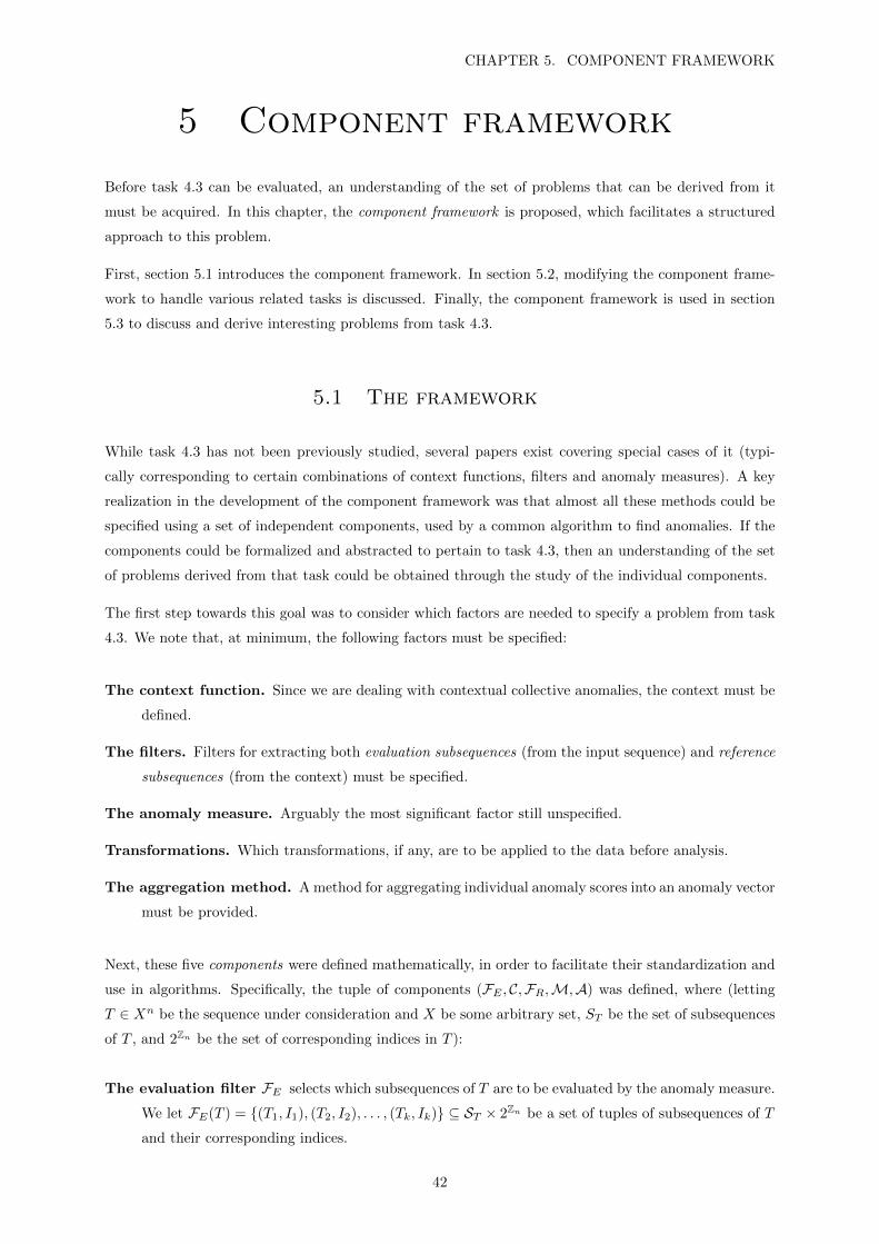
CHAPTER 5. COMPONENT FRAMEWORK

5 Component framework

Before task 4.3 can be evaluated, an understanding of the set of problems that can be derived from it

must be acquired. In this chapter, the component framework is proposed, which facilitates a structured

approach to this problem.

First, section 5.1 introduces the component framework. In section 5.2, modifying the component frame-

work to handle various related tasks is discussed. Finally, the component framework is used in section

5.3 to discuss and derive interesting problems from task 4.3.

5.1 The framework

While task 4.3 has not been previously studied, several papers exist covering special cases of it (typi-

cally corresponding to certain combinations of context functions, filters and anomaly measures). A key

realization in the development of the component framework was that almost all these methods could be

specified using a set of independent components, used by a common algorithm to find anomalies. If the

components could be formalized and abstracted to pertain to task 4.3, then an understanding of the set

of problems derived from that task could be obtained through the study of the individual components.

The first step towards this goal was to consider which factors are needed to specify a problem from task

4.3. We note that, at minimum, the following factors must be specified:

The context function. Since we are dealing with contextual collective anomalies, the context must be

defined.

The filters. Filters for extracting both evaluation subsequences (from the input sequence) and reference

subsequences (from the context) must be specified.

The anomaly measure. Arguably the most significant factor still unspecified.

Transformations. Which transformations, if any, are to be applied to the data before analysis.

The aggregation method. A method for aggregating individual anomaly scores into an anomaly vector

must be provided.

Next, these five components were defined mathematically, in order to facilitate their standardization and

use in algorithms. Specifically, the tuple of components (FE , C,FR,M,A) was defined, where (letting

T ∈ Xn be the sequence under consideration and X be some arbitrary set, ST be the set of subsequences

of T , and 2Zn be the set of corresponding indices in T ):

The evaluation filter FE selects which subsequences of T are to be evaluated by the anomaly measure.

We let FE(T ) = (T1, I1), (T2, I2), . . . , (Tk, Ik) ⊆ ST × 2Zn be a set of tuples of subsequences of T

and their corresponding indices.

42


The context function C is responsible for selecting the appropriate context for subsequences. For-

mally, for (Ti, Ii) ∈ Fe(T ), C(Ii) ⊂ ST gives one or more subsequences constituting the context.

The reference filter FE extracts subsequences from the context to produce a set of reference items.

The anomaly measure M assigns an anomaly score to each of the selected items with regard to their

reference set: M(Ti,FrC(Ii)) ∈ R.

The aggregation function A aggregates the anomaly scores to produce an anomaly vector; i.e. if

S = (ai, Ii)i∈Zkis a vector of anomaly scores and indices for individual elements, then A(S) ∈ Rn.

Finally, an algorithm could be formulated that solves an arbitrary problem specified using this component

framework, as follows:

Require: A sequence T and a tuple (FE , C,FR,M,A).

S ← ∅ . initialize anomaly score container

for (Ti, Ii) ∈ FE(T ) do . iterate over subsequences (and indexes) selected by filter

C ← C(Ii) . acquire context

R← FR(C) . extract reference set from context

S ← S ∪ (M(Ti, R), Ii) . save anomaly score with indexes of subsequence

end for

return A(S) . aggregate scores to form anomaly vector

Restating existing problems within this framework provides several advantages. Firstly, it facilitates

comparison of methods, making it easier to see their similarities and differences. Secondly, it makes it

easy to overview the entire set of problems and propose novel problems based on combinations of existing

components. Finally, the components can be easily interchanged, simplifying method evaluations.

The fact that a single algorithm can be used for all problems suggests the possibility of automated,

accurate handling of diverse data sets. Typically, the extent to which problems can capture anomalies

varies drastically between series from different sources. If this ability could be related to underlying

characteristics of the series, a preliminary analysis could guide the choice of components. Since the

proposed framework simplifies automated analysis and allows for problems to be applied interchangeably

on the same data, it could help both in finding these underlying characteristics and in applying them to

anomaly detection.

As an example of such a characteristic, in [5], various anomaly measures are compared on a task derived

from 3.2 (finding anomalous real-valued sequences in a set of similar sequences) and a correlation is

noted for some problems between the share of anomalies captured and the periodicity of the sequences.

Based on this, investigating links between problem accuracy and characteristics of series in the frequency

domain may prove fruitful.

43


5.2 Related tasks

It is important to note that the component framework is not limited to task 4.3, but can be modified to

handle several related tasks as well. For instance:

Semi-supervised tasks are retrieved by specifying a reference sequence R in addition to the evaluation

sequence T , and letting C(Ti) ≡ R.

Collective anomaly detection tasks are retrieved by specifying C(Ti) = T \ Ti.

Point anomaly and contextual anomaly detection tasks can be retrieved by specifying FE,R(T ) =

(ti)ti∈T and selecting an appropriate context function.

Sequential and frequential tasks need no modifications; they merely require different types of pre-

processing.

Alternative anomaly scores can be retrieved through trivial modifications of the aggregation method

A.

Finding anomalous sequences among a set of sequences mainly requires simplification: FE , C,FR and A can all be ignored for such tasks. The only relevant part is the anomaly measure.

Based on this, the component framework could help elucidate how different sequential anomaly detection

tasks are related. Furthermore, since all derived problems can be solved using a single algorithm when

formulated using the component framework, the implementation and evaluation of a large class of anomaly

detection tasks could be performed relatively easily. Indeed, it would be simple to modify ad-eval (which

implements the component framework) to handle any of the above tasks.

5.3 Components

We now discuss possible choices of the components FE , C, FR, M and A and the implications of these

choices.

While task 4.3 has not been previously studied, components based on existing methods for other tasks

can be used with it. In the following discussion, several such component choices, as well as a few new

components, are mentioned.

5.3.1 The evaluation filter

The evaluation filter takes a sequence and extracts subsequences from it to be used in the analysis. In

the literature, sliding window approaches are almost always taken. In these methods, evenly spaced

subsequences of equal length are extracted from the series:

FE((t1, t2, . . . , tn)) = (t1, t2, . . . , tw), (t1+s, t2+s, . . . , tw+s), . . . , (tα−s, tα−s+1, . . . , tα),

44


where w is the window length, s is the displacement, and α = bns c × w. A constant value of w is almost

always used, since most anomaly measures can not deal with items of varying dimensionality. The value

of s is typically taken to be 1 ≤ s ≤ w. The total number of elements is bn−ws c+ 1, and thus decreases

with larger s.

Other approaches might be appropriate for anomaly measures which support variable-size elements. In

[26], a binary search is performed on T to find discords. Note that such an approach requires a slight

modification of the algorithm given above.

5.3.2 The context function

As mentioned before, several different context functions are plausible for use in sequential anomaly

detection. We have previously mentioned the context (assuming that T = (t1, t2, . . . , tn) is the series

under consideration):

C((ti, ti+1, . . . , tj)) = (ti−m, ti−m+1, . . . ti−1), (tj+1, tj+2, . . . , tj+n),

which we refer to as the symmetric local context if m = n and the asymmetric local context otherwise;

the novelty context :

C((ti, ti+1, . . . , tj)) = (t1, t2, . . . , ti−1);

and the trivial context (for detecting collective or point anomalies):

C((ti, ti+1, . . . , tj)) = (t1, t2, . . . , ti−1), (tj+1, tj+2, . . . , tn).

We also introduce the semi-supervised context, in which C(Ti) ≡ X for some reference sequence X.

Note that the number of elements in the context will typically have a significant impact on analysis time.

While the sizes of the local and semi-supervised contexts are both constant as functions of the sequence

length, the novelty and trivial contexts grow linearly, which is likely to cause problems in large data sets.

5.3.3 The reference filter

The reference filter works like the evaluation filter, but extracts subsequences from the context instead

of from the evaluation series. As with the evaluation filter, it is usually best to use a sliding window as

the reference filter. If the anomaly measure does not require items of equal length, the reference filter

can be ignored, i.e. FR(T ) = T .

5.3.4 The anomaly measure

As is typically the case, the anomaly measure is the central part of any problem derived from task 4.3.

Formally, any anomaly measure that takes an evaluation vector and a set of reference vectors as inputs

45


and returns a real value is a candidate for M. We now discuss a few such anomaly measures, following

the classification in section 2.4.

As previously mentioned, statistical measures are attractive due to the theoretical justification they

provide for anomaly detection. However, there are certain factors which render their use problematic for

the task at hand. Firstly, as discussed in section 4.1 we can not assume that the data belongs to any

particular distribution, so parametric problem formulations are not appropriate.

Since few non-parametric methods for anomaly detection in sequential data take into account either

collective anomalies or context, and since naive approaches are likely to suffer from convergence issues, 1

suggesting appropriate non-parametric methods for task 4.3 is difficult. However, in the case of task 4.1,

point anomalies (for which statistical methods have been extensively researched) are more interesting

than collective anomalies, and statistical methods are likely to be applicable.

Information theoretical measures are potentially interesting for the chosen task. However, most such

methods are essentially distance-based anomaly measures equipped with information theoretical distance

measures. For this reason, we do not cover information theoretical anomaly measures separately from

distance-based measures.

Instead, we emphasize distance-based measures. Since they encompass a wide variety of methods, which

have been shown to be successful for related problems [5], we dedicate section 5.3.4 to discussing them.

Classifier-based measures have also shown promise for related problems [5]. Generally, any one-class

classifier is potentially suitable for the task; see [47] for an exhaustive discussion on this topic. While

one-class classifiers produce binary output, appropriate anomaly vectors can still be produced through a

suitable choice of A.

Predictive model-based measures are also potentially interesting. They are naturally well suited for novelty

detection, since they necessarily implement a novelty context. However, existing predictive model-based

approaches seem to be lacking for the task at hand. In [5], a leading model-based novelty detection

method [17] which uses an autoregressive model was shown to perform poorly on a related task. While

models are important as a means of reducing the computational complexity of methods, they appear

appropriate to consider only as approximations to other anomaly measures.

Distance measures

When dealing with distance-based problems, the choice of distance measure has a profound impact on

which anomalies are detected. As with other aspects of anomaly measures, however, drawing conclusions

about method efficacy through theory alone is difficult; implementing, evaluating, and comparing several

measures will likely prove more instructive.

Possible interesting measures include the Euclidean distance or the more general Minkowski distance;

measures focused on time series, such as dynamic time warping [49], autocorrelation measures [48], or

1For instance, the expectation maximization algorithm for Gaussian mixture models has convergence issues in high

dimensions with low sample sizes.

46


the Linear Predictive Coding cepstrum [46]; or measures developed for other types of series (accessible

through transforms), such as the compression-based dissimilarity measure [26].

Additionally, the choice of distance measure affects how well methods can be optimized. Naive approaches

to distance-based problems typically scale prohibitively slowly, and are not suitable for large amounts of

data. Optimizations typically involve exploiting properties of the distance measure in order to reduce

the number of distance computations (for instance, the commonly used k-d trees algorithm requires the

distance to be a Minkowski metric).

Transformations

Anomaly measures can be combined with one or more transformations of the data extracted by the filters

to speed up the analysis or to facilitate the detection of certain types of anomalies.

One commonly used data transformation is the Z-normalization transform, which modifies a sequence

to exhibit zero empirical mean and unit variance. It has been argued that comparing time series is

meaningless unless the Z-normalization transform is used [29]. However, this is doubtful, as the transform

masks anomalies consisting of subsequences similar to their surrounding data but with different variance

or mean.

Transformations that transform the data into some alternative domain can also be useful. For example,

transformations based on the discrete Fourier transform (DFT) and discrete wavelet transform (DWT)

[31] have shown promise for sequential anomaly detection.

Furthermore, transformations for real-valued data which produce symbolic sequences are very important,

since they enable the application of symbolic approaches (studied in bioinfomatics, for instance) to real-

valued sequences. While several such transformations exist, symbolic aggregate approximation (SAX) [38]

is by far the most commonly used.

5.3.5 The aggregation method

Once the extracted subsequences have been assigned anomaly scores, they must be aggregated before an

anomaly vector can be formed. While little has been written on this subject, it is not difficult to describe

reasonable aggregation methods. It seems clear that all aggregation functions, or aggregators, ought to

have the form

A((a1, I1), (a2, I2), . . . , (ak, Ik)) = (f(ai : 1 ∈ Ii), f(ai : 2 ∈ Ii), . . . , f(ai : n ∈ Ii)),

where Ii are intervals, ai are assigned anomaly scores, and f is some aggregator-specific function acting

on a vector Rn and producing an aggregate score in R. The maximum, minimum, median and mean of

the values in S all constitute reasonable choices of f(S). We will refer to aggregators using any of these

four functions as maximum, minimum, median, and mean aggregators, respectively.

47

CHAPTER 6. EVALUATION

6 Evaluation

As mentioned throughout this report, thorough empirical evaluations on real-world data sets are pivotal

to elucidating the performance characteristics of problems, methods and tasks. In this chapter, two

factors important when performing evaluations are discussed: evaluation data and error measures.

6.1 Evaluation data

For obvious reasons, the choice of evaluation data largely determines the outcome of the evaluation. Since

the spaces of possible evaluation items for most anomaly detection methods are enormous (often Rn for

very large n), there is little hope of performing exhaustive analyses. Furthermore, while only relatively

small subsets of these spaces are typically interesting for any given application, discovering and delimiting

these subsets is usually impossible, due to a limited understanding of the processes underlying the data.

For this reason, it is critical that a set of evaluation items is used, containing as representative a selection

of relevant phenomena exhibited by data items in the application domain as possible. Since such sets can

not be obtained through purely synthetic means (arguably, the existence of a model that could accurately

create such sets would presuppose a level of understanding of the application domain that would render

anomaly detection unnecessary), real-world data must be used.

However, simply obtaining real-world data is not sufficient; if the anomalies in the data are not labeled,

no baseline can be established, and the evaluation is useless. In the context of task 4.3, this means

that, along with each sequence Si = (s1, s2, . . . , sn) in the evaluation set, a reference anomaly vector

Ai = (a1, a2, . . . , an) must be provided, where each ai indicates how anomalous si is.

When appropriate data is unavailable, there are two possible options. The first is to generate both

series and anomalies, in order to create completely artificial sequences. The second is to take unlabeled

real-world data sets and superposition artificially generated anomalies onto them.

Due to how greatly the data set affects the outcome of anomaly detection analyses, the first approach

is not recommended, other than as a means of gaining a qualitative understanding of tasks, problems

or methods. Even if the artificial data appears highly similar to data from the target domain, it is

very unlikely that the ”best” methods for such data and real-world data will be the same. The second

approach, while also problematic, can at least suggest how well methods are able to recognize normal

data from the target domain from anomalous data.

In the initial stages of this project, it was hoped that sufficient data would be obtained by searching the

internet and existing papers on the subject, or by examining sequences of machine data with a domain

expert. However, enough suitable series could not be obtained through these means, and it became

clear that completely artificial data would have to be used in the evaluation. Because such data can

not adequately capture the intricacies of the target domain, a qualitative evaluation of implemented

methods was performed instead. Still, since a major goal of the project was to facilitate evaluations using

real-world data, utilities for performing appropriate evaluations were added to ad-eval.

48


6.2 Error measures

For any evaluation, some way of assessing the accuracy of the produced anomaly vectors is required.

Formally, given a sequence S = (s1, s2, . . . , sn), a reference anomaly vector R = (r1, r2, . . . , rn) ∈ Rn and

a method that takes a sequence as input and produces an anomaly vector A = (a1, a2, . . . , an) ∈ Rn, a

function ε(A,R) : Rn×Rn → R+ is required that assigns a similarity score, or error measure to A based

on how well it approximates R.

Considering the difficulties involved in obtaining any kind of labeled sequences, and the fact that ranking

elements based on relative degrees of anomalousness is even more difficult, it is reasonable to assume

that all reference anomaly vectors are binary: R = (r1, r2, . . . , rn) ∈ 0, 1n. Since any method derived

from task 4.3 produces real-valued output, this means that error measures should work by comparing

one binary and one real-valued vector; i.e. ε(A,R) : Rn × 0, 1n → R+.

Since constant factors do not affect how accurate an anomaly vector appears, any ε(A,AR) should be

invariant under uniform translations and scalings of A. This means that regular real-valued distance

measures (such as the Euclidean distance) are not applicable. This can be avoided by normalizing A—by

scaling and translating it such that all its elements lie in [0, 1]—before computing the distance. For

instance, the normalized Euclidean error εE , given by

εE =

√√√√ n∑i=1

(ai − amin

amax − amin− ri)2

ought to constitute a reasonable choice of error measure. However, since εE is equally sensitive to the

behaviour of A on normal elements as on anomalous elements, how A treats normal elements (which

should not matter unless they have high anomaly scores) can significantly harm the accuracy of this

measure, as we will see in 8.4.

This pitfall can be avoided by converting A to a binary string AB as well, and using a binary distance

between AB and R as the error measure. Since this is equivalent to selecting a set SA of indexes of

elements from A and comparing it to the set SR of indexes of nonzero elements of R, such error measures

can be seen as evaluating the performance of AB on task 2.23, which is reasonable considering the binary

nature of R.

What remains is to decide how AB should be constructed from A and what binary distance measure

to use. Since the individual elements of SR have equal weight, and since the locations of discrepancies

between AB and R are not important, the Hamming distance δH constitutes a suitable choice of distance

measure. Furthermore, AB should be constructed such that ∀i, j ≤ n : ai < aj ∧ i ∈ SA ⇒ j ∈ SA, which

is equivalent to setting a threshold amin ≤ τ ≤ amax and letting AB be given by

AB = (ab,1, ab,2, . . . , ab,n), where ab,i =

0 if ai < τ

1 if ai ≥ τ.

This gives rise to a number of possible AB equal to the number of distinct values of A. We here propose

49


two error measures corresponding to different choices of τ , both based on δH . The equal support error εES

corresponds to setting τ such that |SA| = |SR|, while the full support error εFS corresponds to choosing

the largest τ such that ∀i : i ∈ SR ⇒ i ∈ SA. While other choices (such as choosing the τ that minimizes

δH) might also be appropriate, only these two were selected in order to limit the scope of the discussion.

Since the three error measures proposed above are expected to produce different results, and since they

have not been (to the author’s knowledge) used in the context of series anomaly detection, they should

be evaluated empirically before being used. Such an evaluation is performed in section 8.4.

50

CHAPTER 7. AD-EVAL

7 ad-eval

As stated in the abstract, the development of a software framework for the evaluation of anomaly detection

methods, called ad-eval and available at http://github.com/aeriksson/ad-eval, was a significant

part of the project. In this chapter, the design, development process, and features of ad-eval are

discussed.

Essentially, ad-eval consists of three separate parts: a library implementing the component framework, a

comprehensive set of utilities for evaluating the performance of methods and problem, and an executable

leveraging the library. The entire project is written in Python.

In this chapter, ad-eval is described in detail. The three parts are described in sections 7.1, 7.2, and

7.3, and some of the design choices made in the development of ad-eval are discussed in section 7.4.

7.1 Implemented components

The anomaly detection part of ad-eval (given the Python package name anomaly detection) is a

faithful implementation of the component framework, including the algorithm proposed in section 5.1.

In order to preserve the modular nature of this framework, the individual components are implemented

as autonomous modules, described below.

As there are no real alternatives found in the literature, the sliding window filter is the only implemented

evaluation filter. Since the optimal window width w and step length s depend on the application, both

of these parameters were left to be user-specified.

Since new new context functions can be implemented relatively easily, and since they have a relatively

major impact on the analysis, all previously discussed contexts (specifically, the asymmetric and sym-

metric local contexts, the novelty context, the trivial context, and the semi-supervised context) were

implemented.

As reference filters, a sliding window filter and the identity filter FE(X) = X were implemented, the

latter because it is a better fit for dimension-independent distance measures.

Due to the limited scope of the project, the only implemented anomaly measures (henceforth referred

to as evaluators) were a variant of k-Nearest Neighbors (kNN), in which the distance to the k’th near-

est element is considered, and a one-class support vector machine (SVM). For the kNN evaluator, the

Euclidean distance as well as the compression-based dissimilarity measure [26] and dynamic time warp-

ing [49] distances were made available. Furthermore, the symbolic aggregate approximation (SAX) and

discrete Fourier transform (DFT) transformations were added as an optional pre-anomaly measure trans-

formations. All parameters of the evaluators, distances, and transformations were left for the user to

specify.

Finally, the mean, median, maximum, and minimum aggregators were implemented.

51


CHAPTER 7. AD-EVAL

7.2 Evaluation utilities

The set of possible interesting tests that could be run on problems derived from task 4.3 is considerable.

A large number of component combinations can be used; most components have many possible parameter

values, and it is important to assess how these affect the results; and a large set of methods with various

optimizations and approximations can be proposed. For all of these choices, it is important that accuracy

and performance are properly evaluated.

However, the performance of methods is highly dependent on the characteristics of the data sets to which

they are applied. As mentioned in section 6.1, there is no hope to exhaustively cover the space of possible

evaluation sets. Instead, sample data from the target application domain must be obtained before any

tests are performed. Furthermore, obtaining adequate labeled test data is often difficult, and artificial

anomaly generation must be considered as an option.

With this in mind, it was decided that an evaluation framework should be added to ad-eval to help

facilitate the implementation, standardization, and duplication of accuracy and performance evaluations.

Due to the variety of interesting tests highlighted above, an approach focused on the provision of tools

that assist in scripting custom tests was deemed preferable to one focused on the construction of a single

configurable testing program. To this end, utilities were developed for:

• Saving and loading time series to/from file, with or without reference anomaly vectors.

• Pseudorandomly selecting and manipularing subsequences of series (e.g. for adding anomalies).

• Facilitating the testing of large numbers of parameter values.

• Generating various types of artificial anomalies and superpositioning them onto sequences.

• Calculating the anomaly vector distance measures εE , εES and εFS discussed in section 6.2.

• Facilitating the automated comparison of several problems and methods on individual data sets.

• Automating the collection of performance metrics.

• Reporting results.

• Generating various types of custom plots from results.

With these tools in place, it is simple to write scripts that, for instance, generate large amounts of similar

series containing random anomalies and evaluate the performance of several problems on this data in

various ways.

The tools were included in ad-eval as a separate Python module (called eval utils and located in the

evaluation directory of the repository). This module was used to perform all tests in the evaluation

phase of this project.

52

CHAPTER 7. AD-EVAL

7.3 Executable

To enable the stand-alone use of the anomaly detection package, an executable was added to the ad-eval

repository (called anomaly detector and located in the bin directory of the repository). This executable

is used through a command-line interface and a key:value style configuration file, can perform supervised

or semi-supervised anomaly detection on sequences from files or standard input, and can use any of the

components implemented in anomaly detection.

To avoid having to modify this program every time a component in anomaly detection was changed,

the executable was made unaware of all internal details of that package. Consequently, a command-line

interface capable of configuring the components could not be implemented; instead, a configuration file

parser is used to read and pass the component configuration to anomaly detection.

7.4 Design

The development of ad-eval began at the start of the project. Initially, development efforts focused

on the implementation of a few optimized methods found in the literature, to produce a Splunk app.

However, as the project progressed and the issues discussed in section 1.1 (that most methods were

targeted at subtly different tasks, and that due to lacking evaluations, assessing which methods are really

the ‘best’ is not possible), this approach was recognized as fruitless, and abandoned.

Development then shifted towards an implementation of the component framework, with the goals of

maximizing the ease of implementing and evaluating large amounts of components.

Consequently, modularity was a major focus throughout the development process, achieved through

various means. As mentioned previously, the individual components were separated into independednt

modules. Additionally, the evaluation utilities and the executable were decoupled from the component

framework implementation, interfacing with it through only two method calls. Finally, the decision was

made to distribute the configuration of the component framework implementation, letting each component

handle its own configuration and making the rest of the package configuration-agnostic.

It was a natural choice to write the entire implementation in Python, for several reasons. First, Python

is well suited for small, flexible projects such as ad-eval, thanks to its simplicity and flexibility. Fur-

thermore, a number of great libraries for data mining and machine learning exist for Python, which were

used to accelerate the development. Finally, if ad-eval becomes adopted for real-world use, Python’s

good C integration could be leveraged to write optimized code.

Finally, the evaluation utilities were designed with ease of use and flexibility in mind. For instance, while

classes facilitating test data generation, evaluation, and reporting are provided, their use is optional. As

a result, evaluation scripts could be short and simple—the scripts used in the next chapter are all 30 to

70 lines long—without sacrificing flexibility.

53

CHAPTER 8. RESULTS

8 Results

Due to the lack of appropriate evaluation data mentioned in chapter 6, and in order to limit the scope of

this report, a comprehensive evaluation of the implemented problems could not be performed. Instead, a

preliminary, qualitative evaluation was performed, with the goal of gaining some insight into the relative

performance of problem formulations derived from task 4.3, and demonstrating how ad-eval can be used

to simplify and standardize the process of evaluating anomaly detection problems and methods.

In this chapter, the results of this evaluation are presented. Since distance-based evaluators can be

combined with a wider set of other components than classifier-based or other types of evaluators, and

to keep this report from becoming overly long, the focus was placed entirely on the kNN evaluator

implemented in ad-eval. The performance of this evaluator was investigated through the identification of

all remaining unspecified parameters of the components (FE , C,FR,M,A), and individual investigations

of how these parameters affect the analysis.

Of course, all graphs and data in this chapter were obtained using ad-eval. Since one of the main goals

of the evaluation was to demonstrate how ad-eval can be used to perform standardized evaluations, all

scripts used to obtain the figures and results in this chapter are available in the ad-eval source code

repository. Modifying these scripts to use other data sets or to evaluate other components (such as the

SVM evaluator implemented in ad-eval) is trivial.

8.1 Evaluation approach

Since the number of possible combinations of components and parameter values is enormous (even with the

limited number of components implemented in ad-eval), it was not feasible to include a comprehensive

evaluation of all these combinations in this report. Instead, the components were studied individually,

using a preset configuration and varying individual parameter values. Note that this approach only allows

for the assessment of local characteristics of the parameter space around the specific configuration.

As a second limitation, it was decided that the analysis would be focused on a single artificial sequence,

owing to the lack of proper data sets to evaluate. While a large artificial data set could have been generated

for the evaluation, this would have been counterproductive for several reasons. Specifically, as discussed in

chapter 6, generating data set sufficiently diverse to accurately reflect the characteristics of real-world data

sets in target domain is practically impossible, and creating even a rough artificial approximation would

require substantial effort. Any such data set that could fit within the scope of this project would thus be

severely limited, and would not be appropriate for assessing real-world performance. To highlight these

deficiencies, and to simplify the exposition, it was decided that the focus would be placed on examining

the performance characteristics of problems on a single artificial sequence. Rather than performing

evaluations with different types of artificial sequences, all scripts used in the evaluation were added to

the ad-eval source repository, and were constructed such that performing similar evaluations on new

sequences would be trivial.

54

CHAPTER 8. RESULTS

0 50 100 150 200 250 300 350 400

Sequence

0 50 100 150 200 250 300 350 400

Anomaly vector

Figure 8.1: The standard sequence with corresponding reference anomaly vector.

Before choosing a sequence, there were a few things to consider. Since evaluating a large number of

problem should be possible on modest hardware in short time spans, and since anomaly detection methods

are typically rather slow, the sequence should be short. However, the sequence should still contain both

normal data, homogeneous enough to establish a baseline of ‘normal’ behaviour, as well as an anomaly

that deviates appropriately from this baseline. ”Appropriate”, in this case, means that it should be

relatively easy to detect with most reasonable parameter choices, but difficult enough to be detectable

regardless of the parameter choices. A sequence of length 400 was settled on, generated by a random

walk, with added noise in the range 180 to 220. This sequence, referred to in the remainder of this chapter

as the standard sequence or s∗, is shown in figure 8.1 along with the corresponding reference anomaly

vector a∗.

8.2 Parameter space

When considering the set of problems derived from some task, it can be helpful to regard the set of

variables necessary to fully specify a problem from it as the parameter space of that task. Individual

variables correspond to dimensions in the space, while problems correspond to points. General tasks are

associated with large, high-dimensional parameter spaces while more specific tasks have smaller, more

manageable spaces. Searching for an optimal problem derived from some task for some data set, then,

means searching for a point in the parameter space of the task at which the corresponding problem can

most efficiently find the anomalies in the data set. Equivalently, this can be thought of as an attempt to

minimize some error function over the parameter space.

In this case, the parameter space corresponds to the free parameters of the components C = (FE , C,FR,M,A).

We will denote these by Θ. Assuming that some function A(Θ, s) is provided that solves the problem

corresponding to Θ for a sequence s (or equivalently uses the anomaly detector corresponding to Θ to

evaluate s) and outputs an anomaly vector, the task of finding an optimal problem formulation for some

55

CHAPTER 8. RESULTS

data set S can be seen as the task of finding argminΘE(Θ, S) for some error function E that evaluates

the error of A(Θ, s) for each s ∈ S. Assuming that this error function is a linear combination of the errors

according to some error measure δ of the elements in S, this can be written as

ES,δ(Θ) =∑

(si,ai)∈(S,A)

δ(A(Θ, si), ai).

Given a data set and a set of possible components, this task is relatively straight-forward. While filters,

contexts and aggregators with infinite parameter spaces are possible, the components discussed in this

report have relatively small, finite parameter spaces. This means that an exhaustive search would be

possible in theory.

However, most choices of C will typically have a large number of free parameters, resulting in a high-

dimensional parameter space. This, in combination with the fact that ES,δ(Θ) typically takes a long time

to evaluate, even for small S, renders such exhaustive searches prohibitively computationally expensive

in practice.

8.3 Standard configuration

Due to the limited computational resources available when performing the evaluation, and in order to

simplify the presentation, the parameters had to be studied in isolation. This amounts to studying the

behaviour of ES,δ near a single point in the parameter space by considering its behaviour along orthogonal

lines meeting at this point. This is not sufficient to draw any strong conclusions about global minima of

the error over the parameter space, unless the parameters influence E independently, which is certainly

not the case for task 4.3. However, this is not problematic; the aim of the evaluation was to gain insight

into how the individual parameters affect the outcome, not to find global minima.

The fixed point in the parameter space will be referred to as the standard configuration, and denoted by

Θ∗ = (θ∗1 , θ∗2 , . . . , θ

∗n). The choice of Θ∗ is now described.

As mentioned previously, E was fixed as a kNN evaluator. This evaluator has the free parameters k (which

of the nearest neighbors to use when calculating the anomaly score—set to 1 by default), δ (the distance

function—the standard Euclidean distance δE , by default) and an optional transformation t : Rn → Rm

to apply to the items in the reference set before the evaluation. By default, no transformation is used.

Because the distance measures implemented in ad-eval (except the compression-based dissimilarity mea-

sure) require extracted elements to be of the same length, sliding window filters were the only reasonable

choice. It was thus decided that sliding window filters would be used for both the evaluation and reference

filters, with the free parameters w (window width—10 by default) and s (step length—1 by default).

Since the evaluation was performed on artificial data, there was no reason to use either the novelty

or asymmetric local context. Furthermore, since the trivial context is just a special case of the local

symmetric context (with the context width m set to a maximum), the trivial context was selected to be

the default, with the single free parameter m, set to 400.

56

CHAPTER 8. RESULTS

Finally, since the four aggregators implemented in ad-eval are all parameter-free, it was decided that

the aggregator itself would be treated as a parameter. Since it was assumed that the mean aggregator

would give the most accurate results, it was selected as the default.

In summary, then, the parameter space for this evaluation is parametrized by (k, δ, t, w, s,m,A). To

simplify the following discussion, we will take Θ∗ to be the point where all parameters take on the values

specified above, and let Θ∗α1,α2,...,αnbe the set of points where all parameters except α1, α2, . . . , αn take

on these values (e.g., Θ∗k corresponds to the set of points where all parameters other than k agree with

the standard configuration). We will further denote the set of corresponding anomaly vectors on s∗ as

Aα1,α2,...,αn. The Aα for α = k, δ, t, w, s,m, and A are examined in section 8.5.

8.4 Error measures

10 20 30 40k

10

20

30

40

w

(a) Normalized Euclidean error

10 20 30 40k

10

20

30

40

w

(b) Equal support error

10 20 30 40k

10

20

30

40

w

(c) Full support error

Figure 8.2: Heat maps showing the normalized values of ε(A(Θ∗k,w, s∗), a∗) for the three errors and

k,w = 1, 2, . . . , 50. Blue and red correspond to low and high error values, respectively.

In section 6.2, three error measures for anomaly vectors were introduced: the normalized Euclidean error

εE , the equal support error εES , and the full support error εFS . Since these methods have not been

previously studied with regards to sequential anomaly detection, how well they capture the intuitive

notions of accuracy must be assessed before they can be used to evaluate problem formulations.

Such an assessment was performed by computing and graphing the errors ε(A(Θ∗k,w, s∗), a∗) for ε = εE , εES

and εFS and (k,w) ∈ 1, 2, . . . , 502. Heat maps of these values are shown in figure 8.2. A few of the

Ak,w given the lowest values by each of the error measures were also graphed (figure 8.3.

As shown in the heat maps, the three error measures give similar results, attaining minima and maxima

in the same regions. Since εES and εFS operate on binary strings and thus have discrete domains, they

often assign identical errors to nearby points. This is the cause of the relatively jagged appearance in the

plots of these errors compared to the smoother appearance of the εE plot.

Figure 8.3 shows the anomaly vectors with the nth lowest errors for the three distance measures. All

three measures give similar anomaly vectors for n = 1 and n = 10, with the normalized Euclidean and

full support errors giving the same anomaly vector in both cases. For n = 50 and n = 100, however,

57

CHAPTER 8. RESULTS

n = 1

Equal supportFull supportNormalized Euclidean

n = 10


n = 50


n = 100


Figure 8.3: The nth best Ak,w according to the three error measures for n = 1, 10, 50 and 100.

the full support error seems to prioritize smooth anomaly vectors, while the other two anomaly measures

prioritize anomaly vectors with few false positives.

One interesting aspect evidenced in the heat map plot is that while εES and εFS are both very large for

Ak,w with small w, this tendency is not shared by the Euclidean error. As seen in section 8.5.4, anomalies

significantly larger than w will not be detected by kNN methods, which means that assigning a large

value to these anomaly vectors is reasonable. Since the normalized Euclidean error (unlike the other two

distances) gives equal weight to every component, it will assign relatively low values to anomaly vectors

that only partially capture anomalies as long as most of their elements are close to zero. Indeed, this is

the case for the Ak,w with small w since these anomaly vectors are close to constant everywhere except

for a few spikes.

As an illustration of the potential problems this could cause, see figure 8.4, which shows one reference

anomaly vector and two candidate anomaly vectors for a long sequence. Here, the first anomaly vector,

while noisy, accurately captures the anomaly while the second not only misses the anomaly, but also

introduces two false positives. While εFS and εES are significantly smaller for the first candidate than

for the second, the reverse is true for εE . This problem is amplified as the sequence length grows.

These results indicate that εE should be used with caution, and that since other two error measures are

preferable since they were defined specifically to avoid problems such as this.

58

CHAPTER 8. RESULTS

0 50 100 150 200 250 300 350 400

Reference anomaly vector

0 50 100 150 200 250 300 350 400

Candidate anomaly vector 1

0 50 100 150 200 250 300 350 400

Candidate anomaly vector 2

Figure 8.4: A reference anomaly vector for a long sequence and two corresponding candidate anomaly vectors.The first candidate vector, while noisy, correctly marks the anomaly. The second candidate does not mark theanomaly and marks two false anomalies. εE , εES and εEF for the two sequences are 8.3 and 2.2; 0.010 and 0.99;and 0.0050 and 0.99, respectively.

59

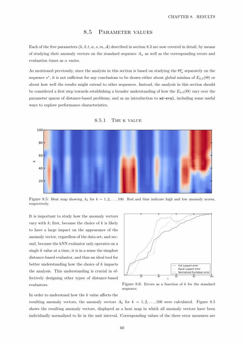
CHAPTER 8. RESULTS

8.5 Parameter values

Each of the free parameters (k, δ, t, w, s,m,A) described in section 8.3 are now covered in detail, by means

of studying their anomaly vectors on the standard sequence Aα as well as the corresponding errors and

evaluation times as α varies.

As mentioned previously, since the analysis in this section is based on studying the Θ∗α separately on the

sequence s∗, it is not sufficient for any conclusions to be drawn either about global minima of Eδ,S(Θ) or

about how well the results might extend to other sequences. Instead, the analysis in this section should

be considered a first step towards establishing a broader understanding of how the Eδ,S(Θ) vary over the

parameter spaces of distance-based problems, and as an introduction to ad-eval, including some useful

ways to explore performance characteristics.

8.5.1 The k value

20

40

60

80

100

k

Figure 8.5: Heat map showing Ak for k = 1, 2, . . . , 100. Red and blue indicate high and low anomaly scores,respectively.

20 40 60 80 100k

Full support errorEqual support errorNormalized Euclidean error

Figure 8.6: Errors as a function of k for the standardsequence.

It is important to study how the anomaly vectors

vary with k; first, because the choice of k is likely

to have a large impact on the appearance of the

anomaly vector, regardless of the data set; and sec-

ond, because the kNN evaluator only operates on a

single k value at a time, it is in a sense the simplest

distance-based evaluator, and thus an ideal tool for

better understanding how the choice of k impacts

the analysis. This understanding is crucial in ef-

fectively designing other types of distance-based

evaluators.

In order to understand how the k value affects the

resulting anomaly vectors, the anomaly vectors Ak for k = 1, 2, . . . , 100 were calculated. Figure 8.5

shows the resulting anomaly vectors, displayed as a heat map in which all anomaly vectors have been

individually normalized to lie in the unit interval. Corresponding values of the three error measures are

60

CHAPTER 8. RESULTS

shown in figure 8.6. Note that this plot shows only relative errors, as the three error graphs have been

individually normalized to the unit interval.

20 40 60 80 100k

0.0

0.5

1.0

1.5

2.0

2.5

time (s)

Figure 8.7: Evaluation times when varying k on thestandard sequence.

Finally, figure 8.7 shows the computation times for

calculating the anomaly vectors Ak. Since the im-

plemented kNN method operates by brute force,

the entire reference set must be evaluated regard-

less of k, so the constant evaluation time exhib-

ited in this figure is expected. For any distance

measure that is a metric, such as the Euclidean

distance, more efficient methods exist.

The smoothness with which the Ak vary with k

indicate that using several nearby k in distance-

based evaluators is not likely to significantly im-

prove accuracy. Furthermore, at least in this case,

k = 1 minimizes all three error measures, and there is no indication that considering additional k might

help. While higher k do lead to other regions being marked as anomalous, these regions do not correspond

to relevant features. If this holds in general, there is no need to consider k higher than 1, and using linear

combinations of several k is not likely to lead to any significant increase in accuracy. However, a much

more thorough evaluation is required before any conclusions can be drawn.

8.5.2 The distance function

20

40

60

80

100

k

Euclidean

20

40

60

80

100

k

DTW

Figure 8.8: Heat maps showing Ak,δ for the Euclidean and DTW distances.

For obvious reasons, the choice of the distance function δ can have a great impact on the anomaly vectors

when using distance-based methods. The distance measures implemented in ad-eval are the Euclidean

distance, the dynamic time warp (DTW) distance, and the compression-based dissimilarity measure

(CDM). To investigate the relative performance of these, the anomaly vectors Ak,δ were examined. Note

that since Aδ consists of only one value per distance measure, calculating only Aδ would have yielded

61

CHAPTER 8. RESULTS

insufficient data.

The ad-eval implementation of the CDM performed poorly. To begin with, it ran significantly slower

than the other methods, rendering any comprehensive analysis impossible. Furthermore, it produced

poor anomaly vectors. There are a few possible explanations for this. First, the z-normalization step

of the SAX transformation (in which each extracted subsequence is given zero empirical mean and unit

variance) leads to poor results on random data regardless of the distance measure. Secondly, the window

width of 10 used in the standard configuration means that the extracted sequences are short and can

not be efficiently compressed, leading to a roughly constant distance value. While the CDM will likely

perform better and with other parameters, it was decided that the CDM would not be investigated further

due to its slowness.

20 40 60 80 100k

Full support

DTWEuclidean

20 40 60 80 100k

Equal support

DTWEuclidean

20 40 60 80 100k

Normalized Euclidean

DTWEuclidean

Figure 8.9: Errors for Ak,δ.

Instead, the focus was placed on comparing the

Euclidean and DTW distances. Heat maps of the

resulting anomaly vectors are shown in figure 8.8

and a plot of the corresponding errors is shown in

figure 8.9. As is seen in the heat map, there is gen-

erally little difference between the outcomes of the

two distance measures; the DTW distance gives

slightly ‘cleaner’ (i.e., with non-anomalous regions

closer to 0) anomaly vectors for very low values of

k, while the Euclidean distance assigns a slightly

lower score to the false anomalies encountered at

high values of k. While there are some differences in the obtained errors—the DTW distance gives a

better normalized Euclidean error, while the Euclidean distance generally gives better values of the other

two errors—the evaluation is not sufficient to draw any conclusions about the relative merits of the two

measures.

However, the fact that the DTW distance does not perform worse than the Euclidean distance in this

evaluation is interesting. Since the DTW was designed to recognize long, shifted but relatively similar

continuous sequences, it might be expected to perform poorly on other types of data, such as the short,

random data used in this evaluation. The fact that this is not the case is a positive indication.

62

CHAPTER 8. RESULTS

8.5.3 Transformations

20

40

60

80

100

k

None

20

40

60

80

100

k

DFT

Figure 8.10: Heat maps of the Ak,t for k = 1, 2, . . . , 100 with and without the discrete Fourier transform.

As discussed in chapter 3, applying transformations to extracted subsequences prior to evaluation, such

as to perform dimensionality reduction, might assist in discovering certain types of anomalies. While a

large number of compressions and other transformations deserving investigation have been proposed, due

to time constraints, only the discrete Fourier transform (DFT) was implemented in ad-eval.

The performance of the DFT was investigated by evaluating the standard sequence for k = 1, 2, . . . , n with

and without the DFT. A heat map of the results is shown in figure 8.10, and a plot of the corresponding

errors is shown in figure 8.11.

20 40 60 80 100k

Full support

NoneDFT

20 40 60 80 100k

Equal support

NoneDFT

20 40 60 80 100k

Normalized Euclidean

NoneDFT

Figure 8.11: Errors of the Ak,t.

While the DFT gave fairly accurate anomaly vec-

tors for low values of k, it performed poorly over-

all, returning less accurate anomaly vectors and

higher error values over all k. This is reason-

able: the DFT is not expected to perform well on

random data. A proper evaluation of the perfor-

mance characteristics of kNN methods using the

DFT would require a more diverse data set.

63

CHAPTER 8. RESULTS

8.5.4 The sliding window width

10

20

30

40

50

w

Figure 8.12: Heat map of the Aw for w = 1, 2, . . . , 50.

10 20 30 40 50w


Figure 8.13: Errors for the anomaly vectors Aw.

Since w, the sliding window width, determines the

size of the elements used by the evaluator, it should

have a significant impact on the size of detected

features. To determine if this was the case, the

anomaly vectors Aw for w = 1, 2, . . . , 50 were

computed and examined. The results are shown

in figures 8.12, 8.13, and 8.14.

As seen in the figures, very low values of this

parameter are associated with a very high error.

This is expected, since as w tends to 1, the target

anomaly type is reduced to point anomalies. Fur-

thermore, all errors increase sharply as w nears 20, indicating that large values of w lead to inaccurate

results.

20 40 60 80 100w

0.0

0.5

1.0

1.5

2.0

time (s)

Figure 8.14: Evaluation times for the anomaly vectorsAw.

Interestingly, the plot in figure 8.12 shows that be-

yond w ≈ 3, increasing w essentially amounts to

smoothing the resulting anomaly vectors. Since

the anomaly in the standard sequence has a rela-

tively small width of 40, and since its surroundings

have low anomaly values for low values of w, this

could help explain why the anomaly is not detected

after w ≈ 40.

It is further interesting to note that while the er-

rors are at a minimum when w ≈ 5, the anomaly

vectors in this area contain three separate spikes

in the vicinity of the anomaly, rather than a single

smooth bump. Arguably, the anomaly vectors at w ≈ 10 are preferable, since they more clearly mark

the anomaly. This suggests that the error measures may need refinement.

Finally, while the evaluation time ought to be roughly independent of w (or proportional to the evaluation

64

CHAPTER 8. RESULTS

time of the distance metric with vectors of length w), figure 8.14 shows a decrease in the evaluation time

as w grows. This is likely due to the fact that the relatively small width of the evaluation sequence means

fewer elements are evaluated as w grows. An evaluation performed on a long sequence, in which the

evaluation filter operates on the middle of the sequence while the reference filter operates on the entire

sequence, could be used to confirm this.

8.5.5 The sliding window step

1

2

3

4

5

6

7

8

9

10

s

Figure 8.15: Heat map of the anomaly vectors As for s = 1, 2, . . . , 10. Note that no major false anomalies occurfor s < 8.

1 2 3 4 5 6 7 8 9 10s


Figure 8.16: Errors of the anomaly vectors As.

1 2 3 4 5 6 7 8 9 10s

0.0

0.5

1.0

1.5

2.0

time (s)

Figure 8.17: Evaluation times for the As. As expected,the graph indicates that the times are O(1/s2).

The sliding window step, s, is interesting mainly for the large effect it has on the execution time. For a

brute-force kNN evaluator with the trivial context and sliding window filters, the number of comparisons

performed on a sequence of length L is Θ((L/s)2). It is therefor desirable to choose a value of s that is

as large as possible. However, it is likely that all three errors increase with s for all sequences, and large

s values might lead to poor results.

To gain some insight into the performance of kNN methods for higher s, the anomaly vectors As were

computed for s = 1 to 10 (the value of w is 10 in the default configuration). The results are shown in

figures 8.15, 8.16, and 8.17.

As seen in figure 8.15, the anomaly vectors are fairly accurate for all s. No major false anomalies are

65

CHAPTER 8. RESULTS

exhibited for s < 8, and the actual anomaly is still clearly detected over all s. This is reflected in the

errors in figure 8.17: all errors are low until s ≥ 8. Additionally, the evaluation time plot follows the

expected O(1/s2) trend.

In light of these results, perhaps a multi-resolution scheme should be considered, in which a preliminary,

‘coarse’ evaluation (corresponding to high s), and a ‘fine’ evaluation (corresponding to low s) is per-

formed only on those subsequences which are given the highest anomaly scores in the coarse evaluation.

Depending on how the subsequences for the fine evaluation are selected, and on the context type, such

an algorithm could achieve either lower computational complexity or an evaluation time reduction by a

constant factor. If, as indicated in this evaluation, false positives but no false negatives are introduced as

s increases, fine evaluation would only rule out false anomalies, and there would be no loss of analytical

power.

8.5.6 The context width

50

100

150

200

250

300

350

m

Figure 8.18: Heat map of the Am for m = 20, 21, . . . , 400. Note the false anomaly present at the left end of theanomaly vectors until m ≈ 330.

50 100 150 200 250 300 350m


Figure 8.19: Errors of the anomaly vectors Am.

Which values of the context width m are appropri-

ate depends heavily on the application domain and

on the types of anomalies present in the data. Ide-

ally, the importance of the context width should be

evaluated by considering several sequences with a

natural context concept, such as the bottom series

in figure 2.4. Constructing representative artificial

data sets of such sequences is likely to be difficult,

so real-world series should be used for such an eval-

uation.

While such data sets are not available, a simple

evaluation on the available data can still prove illuminating. The standard sequence is highly homogeneous

and has no natural contexts. Thus, all errors should be expected to decrease monotonically with increasing

m. To confirm this, the anomaly vectors Am were computed for m = 20 to 400. The results of this

evaluation are shown in figures 8.18, 8.19, and 8.20.

66

CHAPTER 8. RESULTS

As these figures demonstrate, the anomaly vectors identify a false anomaly at the left end until m ≈ 330,

at which point the false anomaly disappears and the errors decline sharply. That this false anomaly

appears for small context widths is understandable since, as seen in figure 8.1, the sequence includes

values at its left end that are not seen again until the right end. As expected, the error is minimized

when the trivial context (corresponding to m > 390) is incorporated.

50 100 150 200 250 300 350m

0.0

0.5

1.0

1.5

2.0

time (s)

Figure 8.20: Evaluation times of the anomaly vectorsAm.

Finally, it should be noted that while the size of the

reference set, and consequently the evaluation time,

grows linearly with the size of the context, the av-

erage context size only grows linearly with m when

m is much smaller than the sequence length. When

m is close to the sequence length, the context size

for a large portion of the subsequences extracted by

the evaluation filter will be limited by the sequence

edges. This leads to the curve in figure 8.20.

67

CHAPTER 8. RESULTS

8.5.7 The aggregator

To get an idea of how the choice of aggregator affects the analysis, the anomaly vectors Ak,A were com-

puted and analyzed for the minimum, maximum, median and mean aggregators, with k = 1, 2, . . . , 100.

Heat map plots of the results are shown in figure 8.21, and plots of the corresponding error measures are

shown in figure 8.22. Single anomaly vectors for k = 1 are shown in figure 8.23.

As seen in figures 8.22 and 8.23, the min and max aggregators produce blockly, piecewice constant

anomaly vectors, while the mean aggregator (and, to a lesser extent, the median aggregator) produces

smooth, continuous anomaly vectors.

0 50 100 150 200 250 300 350 400

20

40

60

80

k

max

0 50 100 150 200 250 300 350 400

20

40

60

80

k

min

0 50 100 150 200 250 300 350 400

20

40

60

80

k

mean

0 50 100 150 200 250 300 350 400

20

40

60

80

k

median

Figure 8.21: Heat maps showing Ak,A for the four aggregators.

As could be expected, the minimum aggregator consistently led to the highest values of εFS . It is likely

to give a low score to a point if a single element containing that point has a low anomaly score, which

effectively means that parts of anomalies will tend to be undervalued—something the full support error is

68

CHAPTER 8. RESULTS

sensitive to. In contrast, the maximum aggregator consistently led to the lowest support error values. This

is also as expected, since max will assign high values to any point contained in an anomalous subsequence.

The median and mean aggregators performed roughly equally well—while the mean performed better for

higher k, this is not relevant; both aggregators were very far off for higher k.

0 20 40 60 80 100k

0.00.10.20.30.40.50.6

error

Full support error

maxminmeanmedian

0 20 40 60 80 100k

0.00

0.05

0.10

0.15

0.20

0.25

error

Equal support error

maxminmeanmedian

0 20 40 60 80 100k

3456789

10

error

Normalized Euclidean error

maxminmeanmedian

Figure 8.22: Errors of the anomaly vectors Ak,A.

Similar, but less clear, results were obtained for the equal support errors. The minimum aggregator

consistently performed the worst with low k, while the maximum aggregator performed the best, on

average, with k up to 40. Again, the mean and median aggregators performed too similarly for any

conclusions to be drawn on their relative merits.

0 50 100 150 200 250 300 350 400

maxminmeanmedian

Figure 8.23: Plot of the Ak,A for k = 1.

Finally, the normalized Euclidean error gives almost

indentical values to the mean and median aggrega-

tors, but exhibits a clear preference for the min-

imum aggregator over the maximum aggregator.

This is likely a consequence of the fact fact that the

minimum aggregator tends to assign scores close to

zero to all elements except for a few, while the max-

imum aggregator tends to assign scores close to zero

to only a few elements. As discussed in section 8.4,

the normalized Euclidean error has a bias in favor

of anomaly vectors where most elements are close to

zero, unlike the type of anomaly vectors produced

by the maximum aggregator.

69

CHAPTER 8. RESULTS

In conclusion, all aggregators performed roughly equally well on s∗ (arguably, the minimum aggregator

performed slightly worse than the others). If this holds in general, then it appears that the choice of

aggregator is mainly one of aesthetics.

70

CHAPTER 9. DISCUSSION

9 Discussion

We conclude this report with a short post-mortem and a discussion of future work.

9.1 Post-mortem

Overall, the project was successful. The new theory introduced in the form of the tasks and problems

and component frameworks has made reasoning about and evaluating problems, as well as proposing

novel problems and methods, significantly easier. Additionally, ad-eval has shown that the component

framework can be effectively implemented and used to easily compare problems and methods. Further-

more, the evaluation utilities and evaluation scripts in ad-eval have shown that performing objective,

reproducible method evaluations that can be reused with different data sets need not be difficult. Finally,

as summarized in the next section, the project illuminated several new frontiers for future work.

However, there were some shortcomings. Since the initial focus on the implementation and evaluation

of a few specific methods was not recognized as inappropriate until these methods had been partially

implemented and large sections of the report had been written, and since the subsequent way forward

was initially unclear, much of the work performed for the project was ultimately discarded.

Moreover, a proper evaluation of the methods implemented in ad-eval was beyond the scope of the

project. While mitigated by the fact that the qualitative evaluation performed in chapter 6 and the

reusable evaluation scripts and utilities added to the repository will greatly facilitate such an evaluation

once appropriate data sets are obtained, this rendered the project goal of finding the problem formulations

most appropriate for the target domain only partially achievable.

9.2 Future work

As repeated throughout this paper, there remains much work to be done on task 4.3 and related tasks,

as well as on ad-eval. A few potential areas in which such work would be useful are now highlighted.

9.2.1 Evaluation

As mentioned several times in this paper, the evaluation performed as part of this project, alone, cannot

conclusively answer which methods are appropriate for the target domain. As indicated in section 6.1,

preferably labeled data from the target domain should be used in the evaluation. However, such data

could not be obtained, so a qualitative evaluation of how parameter and component choices affect the

output anomaly vectors was performed. Once appropriate evaluation data is obtained, several interesting

questions could be answered.

71


First, the tests performed as part of the evaluation in this project should be re-run on a more diverse

data set, to see if the conclusions made in chapter 6 hold in general. Second, a larger portion of the

parameter space should be evaluated. To mitigate the difficulties caused by the very long evaluation times

required for such evaluations, a few modifications should be made to ad-eval. Methods for caching the

results obtained in evaluations, along with tools for parallelizing and distributing evaluations, should be

implemented. Tools for more effectively searching parameter spaces for minima should also be provided.

The relative smoothness with which the output anomaly vectors seem to vary with parameter choices

(at least for the kNN evaluator) could be exploited to avoid a search of the entire parameter space;

methods such as discrete gradient descent combined with random restarts could significantly reduce

the computation time as opposed to a brute-force search, likely without significant loss of accuracy.

Finally, optimizations to the anomaly detection module could potentially lead to large, constant-factor

evaluation speedups.

9.2.2 Performance

Throughout the implementation of ad-eval and the evaluation, performance (in terms of computation

time and memory usage) was deemphasized in favor of accuracy. This was done consciously, in order

to limit the scope of the paper and to avoid the excessive focus on methods and optimizations found in

much of the literature.

Several interesting questions regarding performance warrant investigation. Several types of both pure

optimizations and approximations could be applied to the implemented problem formulations. For in-

stance, multi-resolution algorithms, such as the one suggested in section 8.5.5, could potentially lead to

methods that are both fast and accurate.

Fortunately, the modular nature of ad-eval facilitates the evaluation of optimized methods. Just as

a suite of unit, integration, and performance tests are often run after additions to commercial software

projects, running performance and accuracy tests to evaluate how optimizations affect performance would

be trivial in ad-eval.

9.2.3 Components

Several tasks and problems within the component framework would be interesting to study in more depth.

As shown in chapter 5, there is large potential in suggesting and implementing several new methods within

the component framework. For instance, there exist several anomaly measures and other components in

the literature (including several model-based, artificial neural network-based, and statistical measures,

as well as other distance-based methods and classifiers) that have not been implemented in ad-eval,

and it is likely that some of these will perform better than the implemented components on certain

datasets. Furthermore, several types of transformations should be evaluated (such as the discrete wavelet

transform).

And of course, the parameter spaces of the implemented methods should also be studied in more depth.

It would be especially interesting to examine how the error functions ES,δ(Θ) vary with the evaluation

72


data S. If the minima were to be computed for a large number of sequences from the target domain,

then which problem formulations best suit which kinds of data could be studied from several angles.

9.2.4 Related tasks

As indicated in section 5.2, the components framework could easily be adapted to cover a large number

of related tasks, including the tasks suggested in section 4.3. Evaluations like the one in this paper could

then be performed on these related tasks. It would be especially interesting to compare how individual

components fare on different tasks.

Of course, other tasks would require other types of data, which might be difficult to obtain. However,

the amount of development time required to adapt ad-eval should be minimal.

9.2.5 Deployment

As indicated in section 7.4, ad-eval was designed for eventual use in real-world applications. Due to

its architecture, integration with software such as Splunk would be trivial. Then, the combination of

ad-eval with a good user interface could prove an invaluable tool to monitoring and diagnosis through

anomaly detection in a wide range of application domains.

9.2.6 Ensembles

The components framework might also be used to find correlations between the accuracy of problem

formulations and the underlying characteristics of the data being analyzed, as mentioned in section 5.1.

If such correlations exist, ad-eval could prove instrumental in their discovery due to the ease with which

multiple problem formulations can be applied to, and evaluated in relation to, data sets.

Ideally, this could lead to an ensemble-style approach, in which several methods are combined and weighed

based on their relative suitability to the characteristics of the data.

73


Acknowledgements

I would like to thank Splunk for giving me the inspiration and resources to complete this project; Boris

Chen for his support throughout my internship at Splunk and this thesis; and Konrad Rzezniczak for his

suggestions and help.

I would further like to thank Timo Koski for his help in supervising the project, as well as Chris Conley

for his assistance with the proof-reading of this report.

74

BIBLIOGRAPHY

Bibliography

[1] Curt Monash ”Three broad categories of data.” http://www.dbms2.com/2010/01/17/

three-broad-categories-of-data/

[2] Splunk, Inc. ”Big Data Analytics.” http://www.splunk.com/view/big-data/SP-CAAAGFH

[3] Chandola, Varun, Arindam Banerjee, and Vipin Kumar. ”Anomaly detection: A sur-

vey.” ACM Computing Surveys (CSUR) 41.3 (2009): 15.

[4] Chandola, Varun, Arindam Banerjee, and Vipin Kumar. ”Anomaly detection for dis-

crete sequences: A survey.” Knowledge and Data Engineering, IEEE Transactions on 24.5

(2012): 823-839.

[5] Chandola, Varun. ”Anomaly detection for symbolic sequences and time series data.”

Dissertation. University of Minnesota, 2009.

[6] Hodge, Victoria, and Jim Austin. A survey of outlier detection methodologies. Ar-

tificial Intelligence Review 22.2 (2004): 85-126.

[7] Barnett, Vic, and Toby Lewis. ”Outliers in statistical data.” Wiley Series in Probability

and Mathematical Statistics. Applied Probability and Statistics, Chichester: Wiley, 1984, 3nd (1984).

[8] Hawkins, D. M. ”Identification of outliers.” Monographs on Applied Probability and Statis-

tics, (1980).

[9] Leroy, Annick M., and Peter J. Rousseeuw. ”Robust regression and outlier detec-

tion.” Wiley Series in Probability and Mathematical Statistics, New York: Wiley, (1987).

[10] Bakar, Zuriana Abu, et al. ”A comparative study for outlier detection techniques

in data mining.” Cybernetics and Intelligent Systems, 2006 IEEE Conference on. IEEE, 2006.

[11] Phua, Clifton, Damminda Alahakoon, and Vincent Lee. ”Minority report in fraud

detection: classification of skewed data.” ACM SIGKDD Explorations Newsletter 6.1

(2004): 50-59.

[12] Joshi, Mahesh V., Ramesh C. Agarwal, and Vipin Kumar. ”Predicting rare classes:

Can boosting make any weak learner strong?.” Proceedings of the eighth ACM SIGKDD

international conference on Knowledge discovery and data mining. ACM, 2002.

[13] Dasgupta, Dipankar, and Fernando Nino. ”A comparison of negative and positive

selection algorithms in novel pattern detection.” Systems, Man, and Cybernetics, 2000

IEEE International Conference on. Vol. 1. IEEE, 2000.

[14] Song, Xiuyao, et al. ”Conditional anomaly detection.” Knowledge and Data Engineering,

IEEE Transactions on 19.5 (2007): 631-645.

[15] Eskin, Eleazar, et al. ”A geometric framework for unsupervised anomaly detection:

Detecting intrusions in unlabeled data.” (2002).

75

http://www.dbms2.com/2010/01/17/three-broad-categories-of-data/

http://www.dbms2.com/2010/01/17/three-broad-categories-of-data/

http://www.splunk.com/view/big-data/SP-CAAAGFH

BIBLIOGRAPHY

[16] Basu, Sabyasachi, and Martin Meckesheimer. ”Automatic outlier detection for time

series: an application to sensor data.” Knowledge and Information Systems 11.2 (2007):

137-154.

[17] Ma, Junshui, and Simon Perkins. ”Online novelty detection on temporal sequences.”

Proceedings of the ninth ACM SIGKDD international conference on Knowledge discovery and data

mining. ACM, 2003.

[18] Christos Faloutsos, M. Ranganathan and Yannis Manolopoulos, ”Fast Subsequence Matching in

Time-Series Databases.” Proceedings of the 1994 ACM SIGMOD International Conference on Man-

agement of Data. ACM, 1994

[19] Yi, Byoung-Kee, and Christos Faloutsos. ”Fast time sequence indexing for arbitrary

Lp norms.” Proceedings of the 26th international conference on very large databases, 2000.

[20] Chan, Kin-Pong, and Ada Wai-Chee Fu. ”Efficient time series matching by wavelets.” Data Engi-

neering, 1999. Proceedings., 15th International Conference on. IEEE, 1999.

[21] Ye, Nong. ”A markov chain model of temporal behavior for anomaly detection.”

Proceedings of the 2000 IEEE Systems, Man, and Cybernetics Information Assurance and Security

Workshop. Vol. 166. Oakland: IEEE, 2000.

[22] Blender, R., K. Fraedrich, and F. Lunkeit. ”Identification of cyclone-track regimes

in the North Atlantic.” Quarterly Journal of the Royal Meteorological Society 123.539 (1997):

727-741.

[23] Sekar, R., et al. ”A fast automaton-based method for detecting anomalous program

behaviors.” Security and Privacy, 2001. S&P 2001. Proceedings. 2001 IEEE Symposium on. IEEE,

2001.

[24] Sekar, R., et al. ”Specification-based anomaly detection: a new approach for de-

tecting network intrusions.” Proceedings of the 9th ACM conference on Computer and com-

munications security. ACM, 2002.

[25] Keogh, Eamonn, et al. ”Finding the most unusual time series subsequence: algo-

rithms and applications.” Knowledge and Information Systems 11.1 (2007): 1-27.

[26] Keogh, Eamonn, Stefano Lonardi, and Chotirat Ann Ratanamahatana. ”Towards

parameter-free data mining.” Proceedings of the tenth ACM SIGKDD international conference

on Knowledge discovery and data mining. ACM, 2004.

[27] Keogh, Eamonn, et al. ”Locally adaptive dimensionality reduction for indexing

large time series databases.” ACM SIGMOD Record. Vol. 30. No. 2. ACM, 2001.

[28] Keogh, Eamonn, et al. ”Dimensionality reduction for fast similarity search in large

time series databases.” Knowledge and information Systems 3.3 (2001): 263-286.

[29] Keogh, Eamonn, and Shruti Kasetty. ”On the need for time series data mining

benchmarks: a survey and empirical demonstration.” Data Mining and Knowledge Discovery

7.4 (2003): 349-371.

76

BIBLIOGRAPHY

[30] Geurts, Pierre. ”Pattern extraction for time series classification.” Principles of Data

Mining and Knowledge Discovery (2001): 115-127.

[31] Fu, Ada, et al. ”Finding time series discords based on haar transform.” Advanced

Data Mining and Applications (2006): 31-41.

[32] Bu, Yingyi, et al. ”Wat: Finding top-k discords in time series database.” SDM, 2007.

[33] Yankov, Dragomir, Eamonn Keogh, and Umaa Rebbapragada. ”Disk aware discord

discovery: Finding unusual time series in terabyte sized datasets.” Data Mining, 2007.

ICDM 2007. Seventh IEEE International Conference on. IEEE, 2007.

[34] Lin, Jessica, et al. ”Approximations to magic: Finding unusual medical time series.”

Computer-Based Medical Systems, 2005. Proceedings. 18th IEEE Symposium on. IEEE, 2005.

[35] Venables, William N., and Brian D. Ripley. ch. 5.6 ”Density Estimation” Modern

applied statistics with S. Springer, 2002.

[36] Chan, Philip K., and Matthew V. Mahoney. ”Modeling multiple time series for

anomaly detection.” Data Mining, Fifth IEEE International Conference on. IEEE, 2005.

[37] Warrender, Christina, Stephanie Forrest, and Barak Pearlmutter. ”Detecting in-

trusions using system calls: Alternative data models.” Security and Privacy, 1999. Pro-

ceedings of the 1999 IEEE Symposium on. IEEE, 1999.

[38] Lin, Jessica, et al. ”Experiencing SAX: a novel symbolic representation of time

series.” Data Mining and Knowledge Discovery 15.2 (2007): 107-144.

[39] Morchen, Fabian. ”Time series knowledge mining.” Dissertation. 2006, Philipps-

Universitat Marburg.

[40] Lee, Wenke, and Dong Xiang. ”Information-theoretic measures for anomaly de-

tection.” Security and Privacy, 2001. S&P 2001. Proceedings. 2001 IEEE Symposium on. IEEE,

2001.

[41] Chen, Scott, and Ponani Gopalakrishnan. ”Speaker, environment and channel

change detection and clustering via the Bayesian Information Criterion.” Proc.

DARPA Broadcast News Transcription and Understanding Workshop. 1998.

[42] Radke, Richard J., et al. ”Image change detection algorithms: a systematic survey.”

Image Processing, IEEE Transactions on 14.3 (2005): 294-307.

[43] Jain, Anil K., M. Narasimha Murty, and Patrick J. Flynn. ”Data clustering: a

review.” PACM computing surveys (CSUR) 31.3 (1999): 264-323.

[44] Sandve, Geir Kjetil, and Finn Drablos. ”A survey of motif discovery methods in an

integrated framework.” Biol Direct 1.11 (2006).

[45] Tanaka, Yoshiki, Kazuhisa Iwamoto, and Kuniaki Uehara. ”Discovery of time-series

motif from multi-dimensional data based on mdl principle.” Machine Learning 58.2

(2005): 269-300.

77

BIBLIOGRAPHY

[46] Kalpakis, Konstantinos, Dhiral Gada, and Vasundhara Puttagunta. ”Distance mea-

sures for effective clustering of ARIMA time-series.” Data Mining, 2001. ICDM 2001,

Proceedings IEEE International Conference on. IEEE, 2001.

[47] Tax, David MJ. ”One-class classification.” Dissertation. University of Delft, 2001.

[48] Wang, Changzhou, and X. Sean Wang. ”Supporting content-based searches on time

series via approximation.” Scientific and Statistical Database Management, 2000. Proceedings.

12th International Conference on. IEEE, 2000.

[49] Berndt, D., and James Clifford. ”Using dynamic time warping to find patterns in

time series.” KDD workshop. Vol. 10. No. 16. 1994.

78

TRITA-MAT-E 2013:14 ISRN-KTH/MAT/E—13/14-SE

www.kth.se

anomaly detection in machine-generated data: a …621699/fulltext01.pdf · anomaly detection is an...

Documents