Anno academico 2014/2015

UNIVERSITÀ DEGLI STUDI DI TRIESTE DIPARTIMENTO DI INGEGNERIA E ARCHITETTURA

Corso di Laurea Magistrale in Ingegneria Informatica

Tesi di laurea in

Intelligent technical systems

Un approccio combinato per la rivelazione di anomalie in sistemi di

produzione usando tecniche di machine learning

LAUREANDO RELATORE David Fanjkutić prof. Eric Medvet

CORRELATORI

dott. Alexander Maier

dott. Andreas Bunte

II

III

Abstract

In the present thesis a combined approach is presented for anomaly detection in

production systems using learned system models. It is important mainly because of the

big amount of time and money that could be saved by a fast reaction when a failure

occurs. Usually it is also very time consuming to make a model of the system. An

automated way of modelling is shown using algorithms OTALA (Online Timed

Automata Learning Algorithm) and PCA (Principal Component Analysis) in the context

of model-identification. After identifying the models anomaly detection is computed by

using a distance metric to classify a new observation.

The OTALA+PCA combination successfully detects anomalies, where OTALA also

gives additional information of where did the anomaly occur. Additional expansions to

the proposed approach could be done where the objective would be to identify the cause

of the anomaly.

Riassunto

La presente tesi tratta un approccio combinato per rivelare anomalie in sistemi di

produzione usando modelli costruiti con algoritmi di machine learning. E’ principalmente

importante per via degli enormi risparmi che comporta una pronta reazione ai guasti in

ambienti industriali. Di solito molto tempo viene investito anche nella modellazione dei

sistemi di produzione. Un modo automatico di modellare sistemi è presentato usando gli

algoritmi OTALA e PCA nel contesto di model-identification. Dopo l’identificazione la

rivelazione di anomalie viene eseguita basandosi sulla distanze tra una nuova

osservazione e i modelli appresi.

La combinazione OTALA+PCA è in grado di rivelare anomalie con successo, dove

OTALA dà anche informazione su dove è capitata l’anomalia. Una naturale espansione

all’ approccio proposto avrebbe come obiettivo di trovare la causa delle anomalie

rivelate.

IV

V

nonićima

Neli, Končeti, Stipetu, Zvonku

VI

VII

Table of Contents

1 Introduction ............................................................................................................. 1

2 Idea and objectives .................................................................................................. 2

3 Models – an introduction ......................................................................................... 4

3.1 Automaton ........................................................................................................... 5

3.2 PCA ..................................................................................................................... 6

4 Models – learning algorithms .................................................................................. 7

4.1 PCA ..................................................................................................................... 7

4.2 OTALA ................................................................................................................ 8

4.3 Learning scenario .............................................................................................. 10

5 Anomaly detection ................................................................................................. 12

6 Data acquisition ..................................................................................................... 16

6.1 Energy demonstrator ......................................................................................... 16

6.2 Dataset ............................................................................................................... 17

7 Experiments ........................................................................................................... 19

7.1 Qualitative comparison ...................................................................................... 19

7.2 Quantitative measures ....................................................................................... 24

8 Developed software ............................................................................................... 26

8.1 Parser ................................................................................................................. 26

8.2 Data analyser ..................................................................................................... 27

8.3 Rule generator.................................................................................................... 28

8.4 Plotter ................................................................................................................. 29

9 Conclusion ............................................................................................................. 32

References ...................................................................................................................... 33

Acknowledgments .......................................................................................................... 34

VIII

List of Figures

Figure 1: Data flow concept ............................................................................................. 2

Figure 2: Learning sequence of models ......................................................................... 11

Figure 3: Classification of normal behaviour ................................................................ 12

Figure 4: Anomaly detection scenario ........................................................................... 13

Figure 5: Energy demonstrator ...................................................................................... 16

Figure 6: Energy demonstrator’s high-level process diagram ....................................... 17

Figure 7: Box and Whisker-normal behavior 1 ............................................................. 20

Figure 8: Box and Whisker-normal behavior 2 ............................................................. 21

Figure 9: Box and Whisker-conveyor belt pressed ........................................................ 22

Figure 10: Box and Whisker-ball stolen ........................................................................ 23

Figure 11: Box and Whisker-second ball added ............................................................ 24

Figure 12: Example of a small dataset ........................................................................... 27

Figure 13: Plotter screenshot.......................................................................................... 29

Figure 14: Hue in HSB encoding of RGB ..................................................................... 31

IX

List of Algorithms

Algorithm 1: PCA ............................................................................................................ 8

Algorithm 2: OTALA without time ................................................................................. 9

Algorithm 3: Anomaly detection ................................................................................... 14

X

Terms

Observation– a vector of systems’ measurements at a point in time. The symbol used

throughout the thesis is u(k)

Normal behaviour – an ordered set (by time) of observations that occurred while the

system was functioning normally

Model – an abstract representation of a system learned from normal behaviour

Anomaly – an observation which is not coherent with the learned models. A classifier

will decide if an observation is not coherent with the models

Predicted behaviour – an observation which is not an anomaly

1

1 Introduction

Since the beginning of time human evolution is followed by technological

advancement. It is in our nature to find easier ways of doing things, techniques that are

going to be less time consuming and/or effort consuming than the current ones. In the

modern days human progress reached a point where the work doesn’t have to be done by

individuals any more. Highly complex technical systems are today’s labour power. When

you look in your living room or kitchen and think about the things that you see you will

probably notice that almost all of the things there are actually made by machines. It is

very uncommon that a piece of furniture or any other item present in your home was

made exclusively by human hands, as it once used to be. Clearly in a less personal space

things are even less hand made.

Employers prefer to have workers who work well instead of ones that don’t, of course.

But it is human to make mistakes, so as a consequence there are losses in time and money

for every bad decision or bad performance. That is why supervisors are needed. The work

needs to be controlled and monitored.

The same is with machines. Since automation occupies a major part in today’s

production plants, it is important that it works properly. Failures in automation systems

cause production losses which as an end result cost a lot of money. It is important to

detect them and possibly to detect the cause of the failure. There are multiple ways of

doing so for particular cases, and new effective approaches are always appreciated.

This thesis will discuss one possible approach to formally describe a production

system’s normal behaviour using model-identification algorithms and then use the

obtained models representing the production system to detect anomalies within its

behaviour. After a problem description and giving an insight into work related to the

topic, a more detailed section will introduce the models used in this thesis. The structure

of these models is a starting point for learning simple rules which can then be used as

intuitive references to the expected behaviour of the system.

2

2 Idea and objectives

The aim is to find an effective method to detect anomalies in a production system by

combining the information that can be extracted from models representing it. Data

needed to learn the models is retrieved from the production system and given as input to

multiple learning algorithms such as OTALA, PCA, Clustering and others.

Source: Fraunhofer IOSB-INA

Figure 1: Data flow concept

In the present thesis a distinction is made between low-level data and high-level data.

Low-level data are quantities like energy consumption or signal changes, so technically

measurements obtained using sensors and actions made through actuators. The

algorithms elaborate low-level data and produce high-level data which is then used to

learn the rules for anomaly detection. The anomaly detection algorithm will then

elaborate directly the high-level data.

In a classical approach detecting anomalies would be done already after gathering the

low-level data. The main difference between the classical approach and the approach here

presented is the additional layer of elaboration whose purpose is to abstract the type of

data gathered from sensors and actuators to conceptually obtain an independent layer of

elaboration which will then work exclusively with high-level data, not taking into

consideration the way in which it was constructed nor what type of data is it based on.

The additional layer is not aware of this distinction between the data or the layered

architecture, it treats the high-level data as it would any other data.

3

Using such an approach an abstraction is obtained where the initial data used, the low-

level data, would not be taken into consideration any more. We call the obtained

abstraction “model”. Abstracting the production system using models like automatons for

example, can significantly simplify the understanding of its behaviour because instead of

being a set of physical components, it becomes a set of states which captures better the

different stages of a production cycle. Additionally, automatons for example have a very

intuitive graphical representation.

4

3 Models – an introduction

It is often difficult to understand certain behavioural aspects of production systems, so

many measurements need to be carried out on the physical system. Often a lot of

important measurements are not applicable in practice because of various reasons, for

example the variable that needs to be measured could be inaccessible, like the inner

temperature of an engine.

Given an input a system produces an output. Giving the same input to a model

describing that system can be used to simulate the expected behaviour of the system.

Such models can be used for detecting anomalies. An anomaly is detected when the

system’s behaviour is different from the simulated one. This method of detecting

anomalies is called model-based anomaly detection.

Usually production systems are modelled using Ordinary Differential Equations (ODE)

or Differential Algebraic Equations (DAE), mathematical models that are derived from

physical processes. A model is usually constructed by a domain expert who has a large

theoretical and practical knowledge about the physical system. Depending on the level of

detail needed, the expert makes an appropriately specific model. Low level of detail

doesn’t need a very specific model. Sometimes a very general model suffices, and is

often better than a very detailed one. It is always important to find the right trade-off

between generality and specification to fulfil the requirements of a task.

As stated above, a domain expert is needed to provide the knowledge for modelling

such a system. But is it possible to model a system automatically? Or at least reduce to

some extent the need for a domain expert? This is one of the modern-day challenges, to

give to a machine the knowledge needed to model a system. It is very unlikely that a

machine models a complex system with different discrete and continuous variables and

manages to relate dependencies that exist between them using mathematical modelling.

As an alternative approach there is data-driven modelling which is based on machine

learning techniques.

Using sensors, values of different variables of interest can be measured and saved in a

database or simply logged. Usually data regarding the output of the system is stored and

data regarding the input is usually known. The database will then contain the data

representing the behaviour of the whole system, which is observed as a black box (the

physical structure of the system is not known to the machine). For the purpose of data-

driven modelling the content of the box is not relevant. Data regarding input and output

variables can be used as a training dataset to find the relations between the input and

5

output variables using machine learning (ML) techniques. Since machines do not

understand data, but do know how to elaborate it, this is probably the right direction for

automatizing modelling of production systems.

In machine learning training examples are usually given as vectors in the n-

dimensional Euclidean space. This is arguably the most widely practiced methodology.

However, there are other approaches, such as providing learning information via

relations, constraints, functions, and even models (Japkowicz & Shah, 2011). In the

present thesis a model-based approach to machine learning is proposed where the training

examples will be vectors in the Euclidean space to learn models, and then use those

models as training examples for a rule-based system. The 2 models used are described in

the sequent subsections.

3.1 Automaton

In computer science, an automaton or a finite state machine is an abstract machine used

to solve computational problems. It is usually defined as a 5-tuple in the following way:

Q is a finite set of states.

Σ is a finite set of symbols, called the alphabet of the automaton.

δ is the transition function, that is, δ: Q × Σ → Q.

q0 is the start state, that is, the state of the automaton before any input has been

processed, where q0∈ Q.

F is a set of states of Q (i.e. F⊆Q) called accept states

The current state of an automaton can be retrieved by simulating all the transitions that

occurred starting from the state q0 and given all the symbols (inputs) to the automaton in

the correct sequence. It can be used in various contexts like string matching for example

where an automaton constructed in a particular way will accept certain sequences of

symbols from the alphabet, in order to match particular strings.

A transition function can be seen as a mechanism that reacts to certain inputs and ignores

other. While being in a state, it defines which are the possible input symbols that trigger

the mechanism (transition function) to move from one state to another. Now, there are

multiple alphabets that can be used as the set of acceptable symbols, and they don’t

always have to be alphanumerical. They could be intervals for example or even signals,

see (Niggemann, Stein, Maier, Vodenčarević, & Kleine Büning, 2012). Based on the type

of alphabet that an automaton is partially defined by, there are different types of

6

automata. One of these, the State-based Timed Automata (Maier, 2014), will be discussed

in more detail in Models – learning algorithms chapter.

3.2 PCA

In statistics, Principal Component Analysis is a way of identifying patterns in data.

These patterns are then used to express data so that its similarities and differences are

highlighted. It is usually hard to find patterns in data, especially when it is in a dimension

higher than 3 where graphical representation is not an option, so a human cannot use its

sight and observation capabilities to identify it visually. That is why PCA is a very useful

tool for pattern identification.

Also, beside pattern identification, PCA is useful for dimension reduction. In general,

when data from an n-dimensional space gets mapped to a k<n space, then the data is not

containing the same information any more. More precisely, information is lost due to not

taking into consideration the m=n-k data dimensions that were present in the higher

dimension. The higher is m the more information is lost. But, this loss of information can

be minimized and the data will be transformed to fit the lower dimension space with the

least loss of information by using simple matrix algebra that will be explained in the

Models – learning algorithms chapter.

When performed on a dataset, where the rows are the different observations and the

columns are the different variables of interest, the PCA will identify the most important

variables of that dataset and map them to a lower dimension. In this thesis we refer to the

data in the lower dimension as PCA model. The reason for choosing this model is that the

computational cost of performing anomaly detection (explained in the chapter Anomaly

detection) on a dataset of reduced dimension is lower. It is natural to realize that it is

easier to compute the sum of 2 scalars than of 2 vectors. In this case the latter isn’t that

difficult, but if the vector contains many variables than it is more difficult. And when it is

a matrix is even more difficult, and when it is multiplication instead of sum then even

more.

Now, since the principal aim of the work here presented is to detect anomalies in real-

time, the higher the computational cost the longer it takes to compute it. If it takes too

long then the anomaly would be detected too late, and though not in real-time. For this

reason PCA is used to reduce the dataset by keeping only the most important variables

among hundreds or even thousands of them. A real production plant can easily have a

few thousand of variables of interest, and making a computation among for example 80%

of them really makes a difference.

7

4 Models – learning algorithms

In general, when any algorithm is first developed the author was initially looking for a

systematic solution to a specific problem. That is what an algorithm does actually, that’s

its whole purpose. It is often the case that algorithms are then used in application

scenarios that are different from the originating one. For example if an algorithm can

compute the sum of a number of apples, it can probably perform well enough also when

summing a number boats. Also, the very specific scenario can sometimes be generalized,

like for example instead of summing just apples or boats, it could be generalized to sum

any fruit or transportation vehicle. The other way around is also common because

sometimes some restrictions can be introduced in general algorithms that would make

them perform better on specific cases and maybe give better results.

This chapter will introduce the 2 learning algorithms that are used to learn models that

have origins in a completely different application scenario or were much more general.

The algorithm PCA was originally used for simplification, data reduction and variable

selection. It is now applied also to classification, prediction, unmixing, and 2 more

important for this thesis – modelling and outlier detection (Wold, Esbensen, & Geladi,

1987).

Automata on the other hand has its roots in early computer science where

mathematicians wanted to mathematically describe complex mechanical machines to be

able to understand better their functionality and limitations. We can say that the initial

application scenario for automata was similar to the current one. Other than to give a

formal description (model) of a machine, automata are also used in text processing,

compilers, hardware design, programming languages, artificial intelligence and so forth.

The models are defined in this thesis as abstract representations of a system. The

system can be any production system, so any physical machine that has different

components like conveyor belts, wheels, or any other component. To give a formal

description of a system using only data related to its variables at a given time, 2 data-

driven modelling techniques are used: PCA (for the PCA model) and OTALA (for the

automaton model).

4.1 PCA

An important aspect is that PCA has to be computed on a training set that is describing

only the normal behaviour of the system because on a later step anomaly detection will

be performed, where it has to correctly classify anomalies, so those must not be present in

8

the training set. A more “machine learning” way of saying this would be that only

positive examples are allowed in the training set, so the classifier will later classify as

negative examples (anomalies) all future examples (new observations) that do not fit the

learned model. The learning is done as follows:

(1) Input: highMat

(2) mean = meanPerColumn(highMat)

(3) zeroMeanMat = highMat – mean

(4) covMat = cov(zeroMeanMat)

(5) tranMat = sortEigVecsByEigVals(covMat)

(6) tranMat = chooseNumbOfPC(tranMat)

(7) lowMat = zeroMeanMat * tranMat

(8) Output: tranMat, lowMat

Algorithm 1: PCA

where highMat is the training dataset with columns representing the variables and rows

the observations, tranMat is the transformation matrix which is used to map observations

to the lower dimension, lowMat is the learned PCA model (the training data mapped to

the lower dimension).

Note that tranMat and lowMat have to be saved to be used later for anomaly detection.

The anomaly detection algorithm in chapter Anomaly detection refers to this matrices

with this exact names.

4.2 OTALA

One of the additional supervisors of this thesis, Alexander Maier, has recently

developed the Online Timed Automata Learning Algorithm as part of his PhD

dissertation (Maier, 2014). The algorithm identifies the model of the system by taking

into consideration only its discrete input and output variables. The identified model is

called State-based Timed Automaton.

State-based Timed Automaton It is a 4-tuple A = (S, Σ, T, δ), where S is a finite set of

states. Each state s ∈ S is a tuple s = (id, z), where id is a current numbering and z is an

observation containing only values of the discrete monitored variables.

- Σ is the alphabet, the set of events.

9

- T is a set of transitions. A transition is represented with (s, a, δ, s’), where s, s’ ∈ S

are the source and destination states, a ∈ Σ is the symbol and δ is the clock constraint.

The automaton changes from state si to state sj triggered by a symbol a if the current

clock value satisfies δ. The clock c is set to 0 after executing a transition, so that the

clock starts counting time from executing this transition.

- A transition timing constraint δ: T → I where I is a set of intervals. δ always refers to

the time spent since the last event occurred. It is expressed as a time range or as a

probability density function (PDF), i.e. as probability over time.

Below is the OTALA learning algorithm (without time):

(1) Input: z

(2) Initialize automata = {}

(3) currentState = createNewState(z)

(4) WHILE(not modelLearned)

(5) z = getNewObservation()

(6) FOR(s in States of automata)

(7) IF(z == getSignalVector(s))

(8) stateExists == true

(9) IF(not transitionExists(currentState, s))

(10) createNewTransition(currentState, s)

(11) END IF

(12) END IF

(13) currentState = s

(14) END FOR

(15) IF(not stateExists)

(16) s_new = createNewState()

(17) createNewTransition(currentState, s_new)

(18) currentState = s_new

(19) END IF

(20) END WHILE

(21) Output: automata

Algorithm 2: OTALA without time

where automata is the learned model (a state-based automata), z is the observation

containing only the discrete variables. Since this is an online learning algorithm, the input

z is iteratively fed to the algorithm, until the model is learned.

10

Since the input of the algorithm are discrete values, in the case where there are n binary

variables, the following holds:

2n is the maximum number of states generable by OTALA

It is the case that many of the sensors and actuators of a production system are binary.

Such sensors are most often distance sensors used to indicate the position of a relevant

physical component. On the other hand, binary actuators indicate if a physical component

is active or inactive, like for example is the magnet on, or is the conveyor belt moving.

This data is something that can definitely characterize the different phases in a production

system which makes OTALA a good candidate for modelling production systems.

4.3 Learning scenario

These 2 models are learned in different ways. PCA is learned offline on a final dataset.

That requires that the system runs a number of production cycles to store the observations

from the normal behavior to be accessed later by the PCA algorithm. OTALA on the

other hand is an online learning algorithm which will update its currently learned model

every time that a new signal vector u(k) is observed. The following illustration shows the

scenario:

11

Offline

OnlineOTALA

Is automaton learned?

PCA for each state

Learningcompleted

Turn ON SystemStart

learning

New observation

Logs

NO

YES

N

u(k)

u(k)

Figure 2: Learning sequence of models

where u(k) is the k-th observation, and N represents the normal behaviour of the system.

It is the set of all observations that occurred while the system was functioning normally.

12

5 Anomaly detection

Once that the models have been learned they can be used for anomaly detection. This is

achieved by using a binary classifier that classifies new observations as predicted

behaviour or anomaly. But how does the classifier decide upon an observation if it is an

anomaly or predicted behaviour? The classifier also needs to be learned.

The learning of the 2 models was consisting of multiple phases that involved many

different types and sources of data. On the other hand, we can say that the classifier is

already learned because the data that the classifier needs to make decisions upon is

normally distributed as a pre-processing step in the PCA algorithm. When elaborated

using the anomaly detection algorithm presented in Algorithm 3, all the observations

from the normal behaviour will be classified as predicted behaviour of course, because

the Marr wavelet function used for classification will be given input data that is normally

distributed. The below picture shows values of all observations of the normal behaviour

dataset (later presented in 6.2 Dataset) where the y axis is the output of the Marr wavelet

function and the x axis is the distance of the observation from the origin:

Figure 3: Classification of normal behaviour

13

An idea of how anomaly detection is done is here shown in the below illustration:

Retrieve current state

Map tolower

dimension

Calculate distance fromNormal behaviour

Close enough?

NO

Anomaly!

u(k)Get

corresponding PCA

w(k)

|w(k)|

Figure 4: Anomaly detection scenario

1. A new observation u(k) is used to retrieve the current state of the automaton. The

values of the discrete signals are compared to those that would trigger a state

change. If there is no such transition, the state does not change.

2. The current state SX is used to retrieve the corresponding learned PCA model,

every state of the automaton has a PCA model associated with it

3. The transformation matrix (tranMat) from the corresponding PCA model is used to

map the observation to the lower dimension

14

4. Euclidean distance is then calculated from the normal behaviour (from the origin)

5. A Marr wavelet function is used to classify the new observation:

𝑓(𝒙) =2

√3𝜎𝜋14

∗ (1 −𝑘

𝜎2) ∗ 𝑒

−(𝑘

2𝜎2)

where x is the new observation transformed to the lower space, σ is the standard

deviation, 𝜎2 is the variance, and k is the Euclidean distance from the origin:

𝑘 = √∑ 𝑥𝑖2

𝑑

𝑖=1

where d is the dimension of the lower space.

The anomaly detection algorithm is the following:

(1) Input: u(k), PCA, automata,

(2) currentState = getState(automata, u(k))

(3) PCAcurrentState = getPCA(PCA, currentState)

(4) tranMat = getTranMat(PCAcurrentState)

(5) x = u(k) * tranMat

(6) IF( f(x) > 0 )

(7) classification = predicted_behaviour

(8) ELSE

(9) classification = anomaly

(10) END IF

(11) Output: classification

Algorithm 3: Anomaly detection

where PCA = {PCA𝑖}𝑖=1|𝑆|

is a set of PCA models where each model is associated to one

of the |S| states of automata, where |S| is its number of states, u(k) is the new observation

which is classified as classification.

The distance is measured from the origin because the original data was centred in the

PCA computation by subtracting the mean from each observation. The Marr wavelet

15

function’s particular shape allows to have a natural boundary of zero that simplifies the

classification; an observation is said to be coherent with the normal behaviour if its value,

after being applied to Marr wavelet function, is positive. Otherwise will be classified as

anomaly.

16

6 Data acquisition

In general, production systems include a lot of different sensor types, actuators and

controllers used for controlling and monitoring different components. Monitoring the

condition of a production system requires collecting process data from its sensors and

components and continuously feed this data to the elaboration software. The elaboration

software used in the present thesis is called proKNOWS, developed by Fraunhofer IOSB-

INA, a large research institute in Germany. It is a framework for diagnosis, model

identification and optimization in industrial environments. It is still under development

and not yet implemented in real production plants, but a prototype is implemented in the

Lemgo Model Factory (Modellfabrik, n.d.).

Using proKNOWS data was collected from a physical system called Energy

demonstrator.

Source: Fraunhofer IOSB-INA

Figure 5: Energy demonstrator

6.1 Energy demonstrator

The components are common to all production systems and the signals that are present

are also coherent with the real world scenario. However the number of variables is indeed

a lot smaller than the one in a real production system so the results obtained in this small

testing environment could be different than the ones that would be produced using a more

complex system.

17

The demonstrator’s discrete variables of interest are listed and shown in Figure 5:

Energy demonstrator. The components 1-3 are binary sensors used to determine if the

ball or the magnet head is present. The components from 4-6 are actuators whose values

indicate if the conveyor belt is moving and if so in which direction, and if the magnet is

on. The components 1-6 are all binary.

Additionally, there are 2 other sensors which are continuous. One is used to measure

the power and the other is for energy.

The binary components are used to learn the automaton model using OTALA and the

continuous components are used to learn the PCA model.

The below illustration show the simple processes that are occurring while the

demonstrator is on.

Ball waiting?Magnet head left?

Magnet off?

Magnet on!Move right!

Magnet head right?

Magnet off!Move left!

YES

YES

Figure 6: Energy demonstrator’s high-level process diagram

6.2 Dataset

The data was collected in a total period of 35 minutes. A production cycle for the small

system used (Energy demonstrator) lasts for approximately 8.95 seconds, which means

that the data was collected for approximately 235 production cycles:

- 2 minutes (13 prod. cycles) for learning using OTALA and then offline using PCA

- 33 minutes (222 prod. cycles) for testing normal behaviour and simulated anomalies

18

The system registers an observation approximately every 0.25 seconds, which means

that the automaton was learned on 480 observations (which turned out to be correct). The

PCA was then computed over the same dataset.

For what regards testing, there were 8175 observations that were used to test different

simulated anomalies and to confirm that observations would be classified as predicted

behaviour when anomalies would not be simulated.

The Experiments chapter discusses the approaches taken to test if the classifier is

successful in detecting anomalies.

19

7 Experiments

The testing phase was divided in 15 slots, where each of them was used to test a

different simulated anomaly or a normal behaviour. The results of the experiments are

first going to be interpreted qualitatively and then quantitatively.

7.1 Qualitative comparison

This section will focus on the visual interpretation of the experiments’ results by

showing their graphs and comparing them between them.

7.1.1 Graphs

To give a graphical representation of the overall performance of the classifier, box and

whisker plots are used. To understand these plots 4 elements need to be defined:

1 red line in the blue box represents the median of the data

1 blue box where the bottom and top of it represent the 1st and 3rd quartile of data,

respectively. In fact the interval from the bottom to the median contains 25% of

data, the same amount as the interval from the median to the top of the box

2 black whiskers represent the 2nd and 98th percentile of data – the interval from the

lower whisker to the bottom of the box contains 23% of the data, the same amount

as the interval from the top of the box to the higher whisker, so they both contain a

total of 46% of data

Multiple red crosses represent outliers1 – these are some data points that

accumulate a maximum of 4% of data. Outliers can be located in 2 groups, the 1st

above the higher whisker and the 2nd below the lower whisker where each group

accumulates a maximum of 2% of data

Each of the graphs in the following sections represent 1 of the 15 slots in which the

dataset was divided. In each slot a particular anomaly was simulated or normal behaviour

was tested.

The x axis has only positive discrete values xi ∈ ℕ+ which represent automaton states.

The y axis has continuous values yi ∈ [0, 1] ⊂ ℝ which can be interpreted as a confidence

measure of an observation being part of the normal behaviour. This measure is obtained

by scaling each of the output values of the Marr wavelet function by dividing it by the

highest of all outputs of the function, so that a scaled set is obtained where the element

1 Outliers must not be mixed with anomalies. In this thesis the term outlier will be used only as a point in the box

and whisker graph

20

with the highest value will be 1. This is done to give a more intuitive understanding of the

graphs.

This graph type was chosen because even when the system is function normally there is

always some noise or sensor failure where wrong measures are recorded. When it

happens it is useful to plot outliers because if the number of outliers on the y axis with

value zero is very small in an interval of monitoring, then one can conclude that there

was some noise or sensor failures, instead of anomalies, because anomalies usually come

in groups, not as individual observations. Remember that the system registers an

observation every 0.25 seconds, which means that if the system functions in an

anomalous way for 3 seconds there would be a group (sequence) of 3/0.25 =12

anomalies.

7.1.2 Normal behaviour

To test if normal behaviour is classified correctly 5 slots out of 15 were used. The

optimal expectation was to have all observations classified as predicted behaviour

because no anomalies will be simulated. Since all 5 test slots showed very similar results,

only 2 are shown.

Figure 7: Box and Whisker-normal behavior 1

The graph shows as expected that the number of anomalies is insignificant. Only 2 out

of 545 observations are classified as anomalies. This might be sensor failures or real

21

anomalies, but since anomalies usually come in groups these are probably sensor failures

or measurements affected by noise.

Figure 8: Box and Whisker-normal behavior 2

The 2nd graph shows again a very high accuracy when testing normal behaviour.

7.1.3 Simulated anomalies

Maybe simulated anomalies is not the best name for this chapter. The anomalies were

not simulated in a classical way, where for example an arbitrary observation would be

given as input or an observation that does not deviate too much from the learned models.

The anomalies actually happened for real. The following anomalies were “forced” by

human hand:

The conveyor belt was pressed

The metal ball was taken away from the running magnet head

A second ball was introduced

22

Figure 9: Box and Whisker-conveyor belt pressed

The number of anomalies in states 2 and 3 has clearly increased from the normal

behaviour. Also state 3 shows an increment in the number of observations that are

classified as normal and are relatively further away from the “perfect” normal behaviour.

In fact the bottom of the box is at around 0.80 where in normal behaviour is at around

0.95, not to mention that the whisker reaches 0.7.

The bottom of the box in state 4 reaches even 0.35. The important thing to notice is that

the lower whisker reaches point zero which implies that outliers will not be drawn

because they overlap with it. One conclusion that can be made is that > 2% of data are for

sure anomalies (the outliers). The other is that very probably a little less than 25% of data

are anomalies. This is a heuristic thesis based on the looks of the graphs of the normal

behaviour where all observations in state 4 are classified as predicted behaviour with

confidence 1.

23

Figure 10: Box and Whisker-ball stolen

Simulated anomalies are detected much better in this case than the others. The lower

group of outliers nor the lower whisker is drawn because they overlap with the bottom of

the box which expands to point zero. This means that at least 25% of observations in this

slot are anomalies.

From a high-level perspective this means that a lot of observations differ significantly

from normal behavior. From a low-level perspective, what actually happened, the ball

never arrived at the sensor position which would trigger a transition to a sequent

automaton state. So the automaton remained in state 3 for a much longer time. Since one

of the variables of interest is the energy consumption, as a consequence of being in a state

for a longer period, the value of this variable became too high and not coherent with the

learned model any more.

24

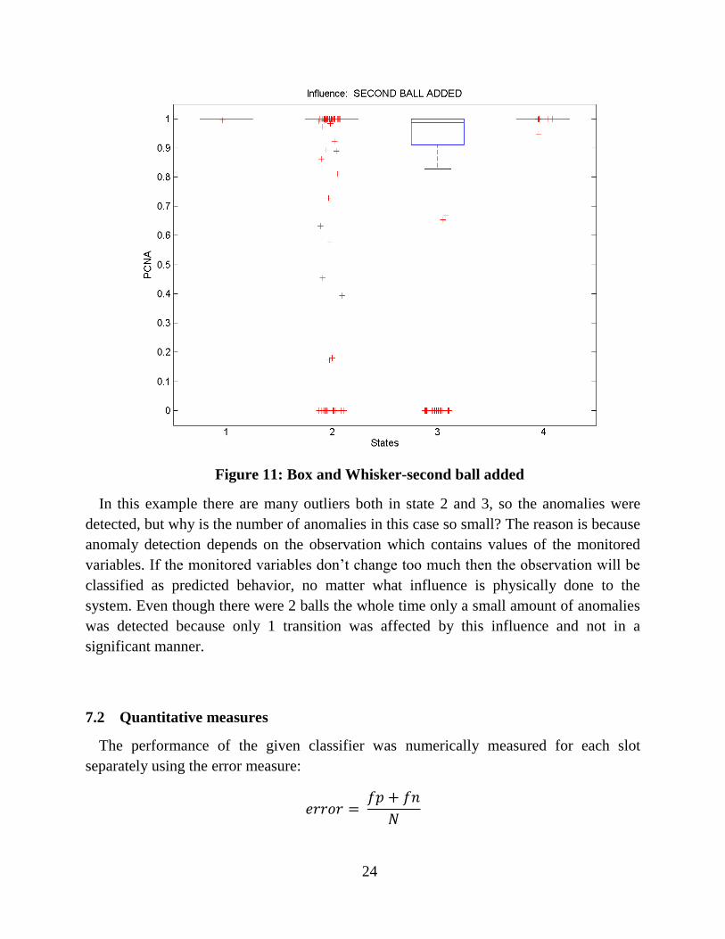
Figure 11: Box and Whisker-second ball added

In this example there are many outliers both in state 2 and 3, so the anomalies were

detected, but why is the number of anomalies in this case so small? The reason is because

anomaly detection depends on the observation which contains values of the monitored

variables. If the monitored variables don’t change too much then the observation will be

classified as predicted behavior, no matter what influence is physically done to the

system. Even though there were 2 balls the whole time only a small amount of anomalies

was detected because only 1 transition was affected by this influence and not in a

significant manner.

7.2 Quantitative measures

The performance of the given classifier was numerically measured for each slot

separately using the error measure:

𝑒𝑟𝑟𝑜𝑟 = 𝑓𝑝 + 𝑓𝑛

𝑁

25

where fp and fn stand for false positive and false negative, respectively. False positives

are observations that are erroneously classified as predicted behaviour, and analogously

false negatives are observations that are erroneously classified as anomalies. The overall

error is given by their sum divided by N, the total number of observations in the slot. The

following table summarizes the results:

Slot fp fn N error(%) accuracy(%)

1 0 40 545 7.3394 92.661

2 0 0 545 0 100

3 0 1 545 0.1835 99.817

4 0 1 545 0.1835 99.817

5 0 3 545 0.5505 99.45

6 2 0 545 0.367 99.633

7 23 4 545 4.9541 95.046

8 19 3 545 4.0367 95.963

9 20 0 545 3.6697 96.33

10 52 8 545 11.009 88.991

11 2 2 545 0.7339 99.266

12 13 5 545 3.3028 96.697

13 9 5 545 2.5688 97.431

14 20 5 545 4.5872 95.413

15 12 1 545 2.3853 97.615

For ease of use the table also contains the accuracy measure:

𝑎𝑐𝑐𝑢𝑟𝑎𝑐𝑦 = 1 − 𝑒𝑟𝑟𝑜𝑟

The slots 1-5 are tests of normal behaviour, which implies that there are no false

positives. Only 1 slot had a significant number of false negatives which could happen

because of multiple reasons, but the most plausible ones are related to sensor failures and

wrong measurements due to noise.

The other 10 slots were used to test different kinds of simulated anomalies described in

the previous chapter. In general, the classifier works very well when classifying predicted

behaviour and a little less well when classifying an anomaly. Still, the overall

performance is very satisfactory.

26

8 Developed software

An additional software module was developed to demonstrate in real-time the

behaviour of the system on a dynamic 2D plot, and to generate rules based on high-level

data, so only on the data retrieved from the learned models. All software was developed

in Java programming language. Two software modules were developed. The first module

consists of 3 main parts: parser, data analyser, rule generator. The second module was

developed to plot in real-time the state of the system.

8.1 Parser

A parser needed to be coded to extract the data logged in a certain format. The

following terms are introduced to refer to the data: A dataset is a text file containing the

records. A record is a line of text in the dataset. The parser extracts the valid records from

the given dataset. A valid record has 1 of the 2 following formats:

TYPE;Date;Time;Timestamp;MODEL_VALUE TYPE;Date;Time;Description

The attribute TYPE can have only 1 of the 4 possible values: DEBUG, ERROR,

WARN or INFO. If the value is DEBUG then the record will have the first format,

otherwise it will have the second one.

Some attributes have a particular meaning. When an error is detected in the behaviour

of the system an ERROR record is generated. WARNING records are analogical. An

INFO record is generated when some input is given through the user interface, like

restarting the learning process of the automaton. The Date and Time attributes describe

the moment in which a record was written to the dataset file. Timestamp is an attribute

describing the moment in which an event actually occurred, or more precisely when the

sensor detected the event. The MODEL_VALUE attribute can have a value which is

characterized by the model in question. The current implementation uses only 2 models:

Automaton and PCNA. Therefore, the MODEL_VALUE attribute can have as value a

PCNA value or an automaton state. To be valid, an automaton state must match the

regular expression S[0-9]+ and a PCNA value must belong to the interval [0,1] ∈ ℝ.

If the record is not valid, for example if the state doesn’t match the regular expression

or the PCNA value is not included in the specified interval or if the format of the record

is not correct, then the record will be ignored and not taken into consideration for the

training of the rules.

27

8.2 Data analyser

Once that parsing is finished data needs to be pre-processed. Records of type INFO,

ERROR and WARN don’t have information about the models; they are used internally

for purposes that are not within the scope of this software module. These records are

filtered out. Only DEBUG records will be used since they carry information regarding the

models. Another useful information is the timestamp of a record, but for now it wasn’t

taken into consideration. As a first approach only data regarding PCNA and automaton

states is used. A relation needed to be found between the 2 models, so first data was

plotted in 2D with states on one axis and corresponding PCNA values on the other. If

system’s behaviour is normal then PCNA values should be close to 1. Since the idea is to

use the generated rules for anomaly detection, the data was collected from a running

system without any intentional rumours so the data would describe the normal behaviour

of the system.

Figure 12: Example of a small dataset

It is easy to notice that the occurrences of PCNA values per each state look like

clusters. Actually the figure is not precise because the abscissa is representing discrete

values so instead of having clusters as “circles” they should be “vertical lines”, so the

representation of a PCNA value is probably not in that exact point, but close to it. For

example all the values that seem to be close to zero in state S4 are actually equal to zero,

which is confirmed in the generated rules in the next chapter. This is because jitter was

added to put some focus on the number of occurrences and not only its value. For

28

example from the density of the clusters it’s easy to see that the system was in state S5

less time than in state S1.

The next step was implementing a clustering algorithm to assign the PCNA values that

are close to one another to the same cluster. This is done because the clusters are later

used to generate rules. For each cluster a rule will be generated, so the actual number of

generated rules will be equal to the number of clusters found by the clustering algorithm.

For this task Weka open source library was used. It offers a lot of different clustering

algorithms. The most suitable one is DBSCAN which, given a dataset, determines the

optimal number of clusters and does the actual clustering based on density. The

DBSCAN class in Weka doesn’t store information regarding cluster assignment. Since

that information is substantial, 3 methods and 2 fields were added to the source code of

the DBSCAN class to retrieve it.

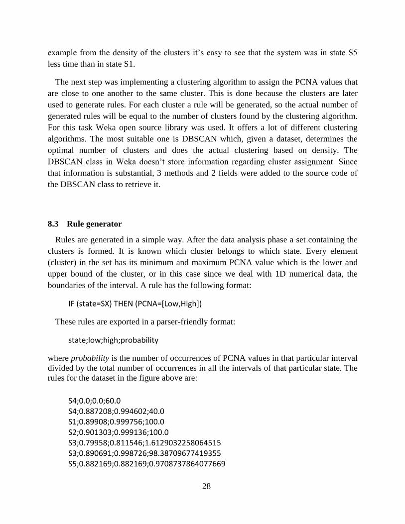
8.3 Rule generator

Rules are generated in a simple way. After the data analysis phase a set containing the

clusters is formed. It is known which cluster belongs to which state. Every element

(cluster) in the set has its minimum and maximum PCNA value which is the lower and

upper bound of the cluster, or in this case since we deal with 1D numerical data, the

boundaries of the interval. A rule has the following format:

IF (state=SX) THEN (PCNA=[Low,High])

These rules are exported in a parser-friendly format:

state;low;high;probability

where probability is the number of occurrences of PCNA values in that particular interval

divided by the total number of occurrences in all the intervals of that particular state. The

rules for the dataset in the figure above are:

S4;0.0;0.0;60.0 S4;0.887208;0.994602;40.0 S1;0.89908;0.999756;100.0 S2;0.901303;0.999136;100.0 S3;0.79958;0.811546;1.6129032258064515 S3;0.890691;0.998726;98.38709677419355 S5;0.882169;0.882169;0.9708737864077669

29

S5;0.901736;0.999093;99.02912621359224 S6;0.0;0.0;5.6105610561056105 S6;0.169788;0.169788;0.33003300330033003 S6;0.900804;0.999382;94.05940594059405

8.4 Plotter

This software module was developed to visualize the behaviour of the system within

the implemented models in real-time. This is possible because each recorded event has its

timestamp which tells us when the event was observed. For now, only 2 models are

implemented, so a 2D graph is suitable. The ordinate represents the PCNA value and the

abscissa represents the state. The plotter is shown below:

Figure 13: Plotter screenshot

Before drawing a point its position needs to be calculated. The following formulas are

used for the x and y coordinates, respectively:

30

𝑥𝑖 = 𝑆 + 𝑠ℎ𝑎𝑘𝑒 ∗ (1 − 2 ∗ 𝑟𝑎𝑛𝑑)

𝑦𝑖 = 𝑃𝐶𝑁𝐴𝑖

where i ∈ ℕ+, S ∈ ℕ0, shake ∈ [0, 0.4], rand ∈ [0, 1].

Variables S and PCNAi are retrieved from the models. It is expected to draw each

PCNA value on the vertical line representing the corresponding state, indicated by the S

variable. But for reasons explained in the second paragraph of chapter 8.2, some noise

was introduced. The shake parameter is set by the user and it describes the maximum

offset, in both directions, from the vertical line representing the state. The rand variable

represents a random number generator which generates from its sequence a

pseudorandom uniformly distributed float value in [0, 1]. In this way more points will be

visible to the user and it is guaranteed that every PCNA value belongs to the state

represented by the closest vertical line. The x coordinate of every point will be in [S-

shake, S+shake]. In the screenshot above the shake variable was set to 0.4, its maximum

value. Theoretically, all values lower than 0.5 guarantee an unambiguous graph, but the

closest the value to 0.5 the harder it is for a human to distinct to which state the value

belongs.

Additionally, each point on the graph has its own colour (it doesn’t have to be unique).

Since this graph represents real-time plotting, a mono-coloured graph would not be very

useful because looking at a single point it wouldn’t be possible to tell the approximate

time when that point was drawn, or in other words when that particular event occurred.

For this reason points are coloured in the following systematic way:

𝑖𝑛𝑐𝑟𝑒𝑚𝑒𝑛𝑡 =𝑚𝑎𝑥𝐻𝑢𝑒

#𝑝𝑜𝑖𝑛𝑡𝑠

ℎ𝑢𝑒𝑖 = 𝑖𝑛𝑐𝑟𝑒𝑚𝑒𝑛𝑡 ∗ 𝑖

𝑐𝑜𝑙𝑜𝑢𝑟𝑖 = 𝐻𝑆𝐵𝐶𝑜𝑙𝑜𝑢𝑟(ℎ𝑢𝑒𝑖 , 100, 100)

where maxHue ∈ {0, 1, …, 359, 360}, #points ∈ ℕ+, i ∈ {1, 2, …, #points}.

The resulting colour is returned by the function HSBColour whose arguments define a

colour in the RGB colour model using the cylindrical-coordinate representation of points

called HSB, where “H” stands for hue, “S” for saturation, and “B” for brightness. In the

current implementation saturation and brightness are set to their maximum values, as a

choice of the developer to simplify the calculations and because a more precise colouring

is not needed for the purpose of the plotter.

31

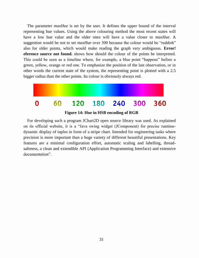
The parameter maxHue is set by the user. It defines the upper bound of the interval

representing hue values. Using the above colouring method the most recent states will

have a low hue value and the older ones will have a value closer to maxHue. A

suggestion would be not to set maxHue over 300 because the colour would be “reddish”

also for older points, which would make reading the graph very ambiguous. Error!

eference source not found. shows how should the colour of the points be interpreted.

This could be seen as a timeline where, for example, a blue point “happens” before a

green, yellow, orange or red one. To emphasize the position of the last observation, or in

other words the current state of the system, the representing point is plotted with a 2.5

bigger radius than the other points. Its colour is obviously always red.

Figure 14: Hue in HSB encoding of RGB

For developing such a program JChart2D open source library was used. As explained

on its official website, it is a “Java swing widget (JComponent) for precise runtime-

dynamic display of tuples in form of a stripe chart. Intended for engineering tasks where

precision is more important than a huge variety of different beautiful presentations. Key

features are a minimal configuration effort, automatic scaling and labelling, thread-

safeness, a clean and extendible API (Application Programming Interface) and extensive

documentation”.

32

9 Conclusion

The proposed approach of combining OTALA and PCA to learn models showed

successful results in detecting anomalies in the given production system, and what is also

important, not to make too many false alarms. But this also depends on the definition of

anomaly. Since in the given production system an observation can be read every 0.25

seconds, it would not be foolish to define as anomaly a sequence of 2 bad observations

instead of just 1, when due to noise or occasional sensor faults anomaly is declared more

often than it actually occurs.

The main advantages and benefits of the approach are the automatic modelling of any

production system without the need of expert knowledge, only using data recorded by

sensors and actuators. Furthermore, the ability to detect different types of anomalies that

is discussed in the Experiments chapter, and one very important feature is the ability to

know in which state of the automaton was the system when the anomaly was detected

which then leads to the actual physical components of the system because the transition

table of the automaton stores information about the discrete sensor values in each state.

One improvement to the proposed approach would be to extend it with an additional

model that would be learned from a different learning algorithm that might give more

potential to diagnosing the exact cause of anomalies.

33

References

Chen, T., & Zhang, J. (2010). On-line multivariate statistical monitoring of batch

processes using Gaussian mixture model. Computers and Chemical Engineering

34, 500-507.

Eickmeyer, J., Li, P., Givehchi, O., Pethig, F., & Niggemann, O. (2015). Data Driven

Modeling for System-Level Condition Monitoring on Wind Power Plants.

Japkowicz, N., & Shah, M. (2011). Evaluating learning algorithms. Cambridge

University Press.

Maier, A. (2014). Identification of Timed Behaviour Models for Diagnosis in Production

Systems.

Modellfabrik. (n.d.). Retrieved 8 14, 2015, from Wikipedia:

https://de.wikipedia.org/wiki/Modellfabrik

Niggemann, O., Stein, B., Maier, A., Vodenčarević, A., & Kleine Büning, H. (2012).

Learning Behavior Models for Hybrid Timed Systems. In Proceedings of the 26th

Conference on Artificial Intelligence (AAAI-12).

Pota, M., Esposito, M., & De Pietro, G. (2013). Transforming probability distributions

into membership functions.

Smith, L. I. (26. 02 2002). A tutorial on Principal Components Analysis.

Solomatine, D., See, L. M., & Abrahart, R. J. (2008). Data-Driven Modelling: Concepts,

Approaches and Experiences. U Computationl Intelligence and Technological

Developments in Water Applications.

Wold, S., Esbensen, K., & Geladi, P. (1987). Principal Component Analysis.

Chemometrics and Intelligent Laboratory Systems, 2, 37-52.

Yina, S., Dingb, S. X., Haghanib, A., Haob, H., & Zhangb, P. (2012). A comparison

study of basic data-driven fault diagnosis and process monitoring methods on the

benchmark Tennessee Eastman process. Journal of Process Control 22, 1567-

1581.

34

Acknowledgments

First of all I need to thank my parents for believing in me and being the best support

that one can possibly have. I made many decisions in my life which they weren’t fond of

but still supported me on every step of the way. I would not be anywhere close to where I

am now if it weren’t for them.

A special thanks goes to my grandmothers and grandfathers who I dedicate this thesis

to. The constant questioning about my exams and academic situation made me sometimes

prepare ahead of a visit, sometimes maybe even more than for an exam. Thank you for

pushing me forward and filling me with positive energy and infinite amounts of delicious

food. You’ve made many things in my life a lot easier.

Thank you Marijana for your limitless love, patience and support throughout our

studies and relationship during almost a third of our lives. I know that you believed in me

the most.

Thank you Alexander and Andreas for numerous technical discussions and for being

more than just supervisors.

Thank you professor Medvet for being always very available and professional. Your

comments helped a lot to shape this thesis.

Thank you Marco for giving me very valuable comments which had an impact on the

thesis itself.

In the end I’d like to thank my fellow colleagues from the course in Computer

Engineering for showing an outstanding collegiality in and out of the classroom. I am

very glad that I’ve been part of such a great team.