anomaly detection on event logs - tu/eanomaly detection on event logs an unsupervised algorithm on...

Eindhoven University of Technology

MASTER

Anomaly detection on event logsan unsupervised algorithm on iXR-messages

Severins, J.D.

Award date:2016

Link to publication

DisclaimerThis document contains a student thesis (bachelor's or master's), as authored by a student at Eindhoven University of Technology. Studenttheses are made available in the TU/e repository upon obtaining the required degree. The grade received is not published on the documentas presented in the repository. The required complexity or quality of research of student theses may vary by program, and the requiredminimum study period may vary in duration.

General rightsCopyright and moral rights for the publications made accessible in the public portal are retained by the authors and/or other copyright ownersand it is a condition of accessing publications that users recognise and abide by the legal requirements associated with these rights.

• Users may download and print one copy of any publication from the public portal for the purpose of private study or research. • You may not further distribute the material or use it for any profit-making activity or commercial gain

https://research.tue.nl/en/studentthesis/anomaly-detection-on-event-logs(7f93395d-182e-4732-ae7d-c0e9257fd7f3).html

ANOMALY DETECTION ON

EVENT LOGS An unsupervised algorithm on iXR-messages

Severins, Eugen [email protected]

07-06-2016

Abstract The goal of this work is to develop an automatic approach to rank machines, or more

specific intervals of events on these machines, based on event characteristics, such that alerts can be raised more effectively. It answers questions such as how data can be represented and how can we relate a ranking to call data. This goal is achieved by

the algorithm proposed in this thesis.

1 / 36

Contents 1. Introduction ..................................................................................................................................... 2

1.1 Description .............................................................................................................................. 2

1.2 Overview of algorithm ............................................................................................................. 2

2. Related work ................................................................................................................................... 4

2.1 Anomaly detection .................................................................................................................. 4

2.2 Unsupervised learning techniques .......................................................................................... 6

2.3 Clustering based local outlier factor (CBLOF) .......................................................................... 7

2.4 Local Density Cluster based Outlier Factor (LDCOF) ............................................................... 7

3. Data representation (Bursts) ........................................................................................................... 9

3.1 Activity of machines ................................................................................................................ 9

3.2 Inter-event-times .................................................................................................................. 10

4. Statistics of bursts ......................................................................................................................... 14

4.1 Calculation of begin and end of a burst. ............................................................................... 14

4.2 Position of error .................................................................................................................... 17

5. Aggregated values over bursts ...................................................................................................... 20

5.1 Number of errors per burst ................................................................................................... 20

5.2 Average position with respect to the beginning of the burst. .............................................. 20

5.3 Average position with respect to the end of the burst. ........................................................ 20

5.4 Average position with respect to the length and the beginning of the burst. ...................... 20

5.5 Number of errors per burst per prefix .................................................................................. 21

6. Clustering on vectors ..................................................................................................................... 22

6.1 Clustering algorithm overview .............................................................................................. 22

6.2 Normalization of the data ..................................................................................................... 22

6.3 Distance Measure .................................................................................................................. 23

6.4 Number of clusters ................................................................................................................ 23

6.5 Result of clustering ................................................................................................................ 25

7. Outlier detection ........................................................................................................................... 28

7.1 Cluster based Local Outlier Factor (CBLOF) ........................................................................... 28

7.2 Local Density Cluster based Outlier Factor (LDCOF) ............................................................. 28

8. Validation by relating call data to clustering ................................................................................. 31

9. Conclusion ..................................................................................................................................... 34

9.1 Future work ........................................................................................................................... 35

10. Bibliography ............................................................................................................................... 36

2 / 36

1. Introduction Philips Healthcare is a manufacturer of medical imaging systems, such as magnetic resonance (MR), interventional x-ray (iXR) and computed tomography (CT) systems, though the focus of this thesis is on

the iXR-systems. These machines produce a lot of data in the form of event logs; messages generated

by the machine and are stored by a host PC, which is part of the iXR-system. This data consists of a

wide variety of error messages. On a daily basis, the data is collected from around the world and stored

in a central database, where the data is to be further analyzed.

One of the problems under consideration in this context is the early detection of performance

problems, in particular, before they actually occur and cause a service call from a hospital to one of

the service centers handling that hospital. When acted upon, early detection of problems may not only

result in fewer calls but also increase the up-time and overall performance of the system. Root cause

analysis, i.e. analysis of problems that have already been reported by the hospital, is another context

under consideration, but it is not part of this study.

1.1 Description To detect possible issues with iXR-systems, we consider both supervised and unsupervised learning

techniques. The unsupervised learning technique has been dubbed anomaly detection (AD); it looks

into anomalies. In data mining, anomaly detection is the identification of items, events or observations

which do not conform to an expected pattern of other items in a dataset [1]. The solution, currently

used by Philips is not necessarily anomaly detection. It focuses on message frequencies and aims to

raise an alert if a frequency grows out of “normal” proportions, where “normal” has a heuristic

definition. We expect that more information is to be gained by the anomaly detection algorithm

proposed in this thesis. The goal of this thesis is:

To develop an automatic approach to rank machines, or more specific intervals of events on these

machines, based on event characteristics, such that alerts can be raised more effectively.

This goal is achieved when we can answer the following four research questions:

1. How can event data from iXR-machines be represented?

2. How can we identify (dis)similarities between bursts of events?

3. How can machines be ranked using the properties of sets of bursts?

4. Is the ranking correlated to the call data?

In the next section, we present an overview of the algorithm developed in order to answer these

research questions and to achieve the research goal.

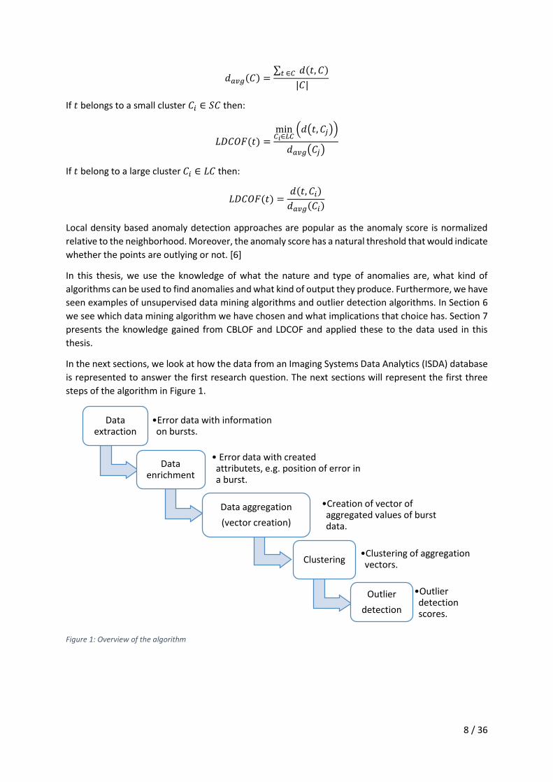
1.2 Overview of algorithm In this section, an overview of the anomaly detection algorithm is given. The successive steps of the

algorithm are illustrated in Figure 1. The first part of the algorithm extracts the data from the database,

in which events are collected from the host PCs by Philips. The event log extracted is further explained

in Section 3. Based on the event log we define bursts, which we interpret as time intervals of

continuous machine activity, which is also part of that section.

The second step uses bursts to define a number of statistics on events with the error category, later

called errors. Definitions such as the position of an error relative to the bounds of the intervals or the

length of a burst are described in Section 4. Furthermore, this is enhanced by defining advanced

properties such as the position relative to the bounds and the length of its respective burst or the

number of errors per type of event.

3 / 36

As discussed in Section 2.2 various unsupervised learning techniques are used to find anomalies. To

apply the chosen unsupervised algorithm, a clustering based anomaly detection algorithm, on these

bursts, we need to aggregate the error statistics, for example taking the average value of the positions

of error. This data aggregation is explained in Section 5 and is the third step of the algorithm. We want

to find anomalous machines instead of anomalous errors, thus, the creation of attributes with

aggregated values is needed. Together with Sections 3 and 4, this will answer the first research

question.

Many data mining techniques or algorithms can then be applied to the resulting aggregation. The

fourth part is the choice (in this case clustering) and application of the chosen data mining algorithm,

will be explained in Section 6 and gives an answer to the second research question.

A typical clustering algorithm provides data instances with labels, but do not predict what label is

anomalous or normal behavior. In the last part of the anomaly detection algorithm, the clustering is

used to provide a ranking in terms of a degree of anomaly. These techniques and the resulting ranking

are found in Section 7. This ranking answers the third research question.

The fourth research question is answered by the validation of the anomaly ranking by relating it to the

registered calls of iXR-machine maintenance. It is, however, not included in Figure 1 as it is not part of

the algorithm.

Figure 1: Overview of the algorithm

In order to answer all the research questions and to achieve the research goal, we first present the

work related to anomalies, anomaly detection and unsupervised data mining algorithms. This is

presented in Section 2.

Data extraction

•Error data with information on bursts.

Data enrichment

• Error data with created attributets, e.g. position of error in a burst.

Data aggregation

(vector creation)

•Creation of vector of aggregated values of burst data.

Clustering•Clustering of aggregation vectors.

Outlier

detection

•Outlier detection scores.

4 / 36

2. Related work The main goal of this thesis is to develop an automatic approach to rank machines, or in this case

intervals of events on these machines, based on event characteristics. This will involve various

aspects of anomalies, anomaly detection and unsupervised data mining algorithms. The explanation

of these aspects is presented in this section.

2.1 Anomaly detection Anomaly detection refers to the problem of finding patterns in data that do not appear to conform to

expected behavior of other elements in the data [1]. Often these anomalies are also referred to as

outliers, exceptions or discordant observations. Anomalies or outliers are terms mostly used in the

computer science context of anomaly detection and are often used interchangeable.

A specific formulation of the problem is determined by several different factors, such as the nature of

the input data, the type of anomaly, the absence of labels and the type of output. These will be

discussed in more detail in the subsequent subsections. It will be used to determine suitable anomaly

detection techniques as parts of the anomaly detection algorithm proposed in this thesis.

2.1.1 Nature of input data Input data is generally a collection of data instances (also referred to as object, record, point, vector,

pattern, event, case, sample, etc. [2] ). In the current context, we consider a collection of log events,

called an event log. Each of these events is described by a set of attributes and in particular that they

are timed are can be of different types. To compare events depending on the type of the attributes,

different methods are used. For example, if the data consists of categorical data specific methods like

a statistical method is needed to compare instances. Nearest neighbor or clustering methods are used

when a distance measure, the ‘closeness’ of two events, is known.

2.1.2 Type of anomaly The second factor is nature of the type of anomaly. Three types are distinguished in [1]:

1. Point anomalies

2. Conditional anomalies

3. Collective anomalies

If an individual data instance is considered as anomalous with respect to the rest of the data, we speak

of point anomalies. An example is found in credit card fraud detection: Assume, for simplicity, the data

is defined by one feature: the amount of money spent. A transaction with this credit card would be

anomalous if the amount spent is very high compared to the normal range of spent money for that

person.

The second type of anomalies are considered conditional: The data attributes of instances are not

anomalous to the rest of the data, but a data instance is anomalous in the context of the dataset [3].

An event can be found anomalous in one context, but an identical event can be considered normal in

another context. Conditional anomalies have been most commonly explored in time-series data [4],

spatial data [5] and [6]. As an example, we look at the monthly temperature in a time-series dataset.

In Figure 2 𝑡1 and 𝑡2 have the same values, however as a low temperature in June is not common

(context) only 𝑡2 is considered an anomaly.

5 / 36

Figure 2: Example of contextual anomaly: 𝑡1 and 𝑡2 have the same value, but only 𝑡2 is only considered an anomaly [1]

The notion of context is found in the structure of the data and has to be specified as part of the problem

formulation. Two attribute types are distinguished: contextual attributes and behavioral attributes.

The first type of attributes describes the ‘neighborhood’ of an instance. For example, in time-series

data, time is a contextual attribute describing the position of the instance in the sequence. The

behavioral attributes describe the non-contextual characteristics of an instance. For example, in spatial

data describing the average number of messages sent per country, the number of messages sent per

city in that country is a behavioral attribute.

If a collection of related data instances is anomalous with respect to the entire data it is termed a

collective anomaly, the third type of anomaly. The individual data instances are not considered

anomalous but together as a collection. In contrast to point-anomalies collective anomalies are not

found in all data sets, but only in sets in which instances are related, for example in time.

2.1.3 Labels The third factor is the type of algorithm used to find anomalies. Three types of algorithm are

distinguished by [1]: Supervised, semi-supervised and unsupervised anomaly detection. Techniques

trained in the supervised detection of anomalous instances assume the availability of labeled training

data. A predictive model is learned on the combination of the attributes of the data instances and its

label. This model is then used to predict unseen or unlabeled data with similar properties. Semi-

supervised algorithms only assume labels on the normal data instances. Normal behavior is modeled

and used to identify anomalous behavior. Lastly, unsupervised anomaly detection algorithms do not

assume that the instances are labeled. It does assume that normal behavior is far more frequent than

anomalous behavior.

2.1.4 Output Typically, the output produced by anomaly detection techniques are one of two types [1]:

scores, techniques that assign an anomaly score to each instance in the test data depending

on the degree to which that instance is considered an anomaly.

labels, techniques that assign a label, either normal or anomalous to each test instance.

6 / 36

2.2 Unsupervised learning techniques Several anomaly detection techniques can be applied to data sets; collections of data instances. One

of the requirements during the graduation project was that only unsupervised learning is to be used.

In the search for unsupervised anomaly detection techniques some basic algorithms are distinguished,

namely, nearest neighbor based, clustering based and probability based anomaly detection algorithms.

The latter is not applicable in this case as we do not have a stochastic model, so it is not discussed in

this thesis.

2.2.1 Nearest neighbor based The concept of nearest neighbor based analysis has been used in several anomaly detection

techniques. Such techniques are based on the assumption that normal data instances occur in dense

neighborhoods, while anomalies occur far from their closest neighbor. These techniques require a

distance or similarity measure defined between two data instances. Broadly speaking two types of

nearest neighbor based techniques are identified:

techniques that use the distance of a data instance to its 𝑘𝑡ℎ nearest neighbor as the

anomaly score, where 𝑘 is a typically small integer, say 10. One example is to use the

sum of the distances from a data instance to all its’ 𝑘 neighbors as the anomaly score

[7], and

techniques that compute the relative density of the neighborhood of each data

instance and use this as the anomaly score. To find the density of a data instance, we

would first find a sphere, centered at the data instance in which the 𝑘 nearest

neighbors are contained. The local density is then computed by dividing 𝑘 by the

volume of this sphere. [8]

A key advantage of nearest neighbor techniques is that they are unsupervised in nature and do not

make any assumptions regarding the generative distribution of the data; they are purely data driven.

However, one of the disadvantages is that nearest neighbor algorithms do not perform well if normal

data instances do not have enough close neighbors, resulting in false positive anomalies. Also, if the

anomalies have close neighbors, a nearest neighbor algorithm will miss anomalies, resulting in false

negatives.

2.2.2 Clustering based Clustering is used to group similar data instances into clusters [2]. It is primarily an unsupervised

technique though semi-supervised algorithms have been explored [9].

Anomaly detection techniques using clustering algorithms are grouped into three categories:

The first category assumes that normal data instances belong to a cluster, while anomalies do

not belong to any cluster. The main disadvantage of these algorithms is that the focus is not

to find anomalies but to find clusters of normal behavior with the anomalies as a by-product.

An example of this is DBSCAN [10].

The second category assumes that normal data instances lie close to their closest cluster

centroid, while anomalies are far away from said centroid. Note that when anomalies in itself

form clusters these techniques will not find these anomalies. K-means clustering is studied by

[11] and is an example of this category.

The third category assumes that normal data instances belong to large and dense clustering,

while anomalies either belong to small or sparse clusters. A variation of techniques has been

proposed by [12].

7 / 36

The advantages of clustering based techniques are that they operate well in unsupervised mode. In

cases in which more complex data types are used they are easily adapted to fit complex data types by

selection of the distance measure and the number of clusters chosen. The testing phase is for clustering

based techniques is fast since the number of clusters against which every test instance need to

compare is a small constant.

Disadvantages of clustering based techniques are that the performance is highly dependent on the

effectiveness of the algorithms in finding the cluster structure and many clustering algorithms detect

anomalies as a by-product and hence are not optimized for anomaly detection.

2.3 Clustering based local outlier factor (CBLOF) An outlier in a dataset is defined informally as a data instance that is considerably different from the

remainders as if it is generated by a different mechanism. The clustering based local outlier factor

algorithm searches for such outliers based on the given clustering. Within each cluster, it reports a

degree of deviation of each data instance in regard to the cluster centroid. [12]

Suppose 𝐶 = {𝐶1, 𝐶2, … , 𝐶𝑘} is the set of clusters provided by a clustering algorithm and are ordered

by size: |𝐶1| ≥ |𝐶2| ≥ ⋯ ≥ |𝐶𝑘|. Given two numeric parameters 𝛼 ∈ [0,1] and 𝛽 ∈ [0,1] and the

dataset 𝐷 we define 𝑏 the smallest boundary of large and small clusters if one of the following formulas

hold:

(|𝐶1 | + |𝐶2 | + ⋯ + |𝐶𝑏 |) ≥ |𝐷| ∗ 𝛼⋁

|𝐶𝑏 |

|𝐶𝑏+1 | ≥ 𝛽

Then the set of large clusters is defined as: 𝐿𝐶 = {𝐶𝑏 | 𝑖 ≤ 𝑏} and the set of small clusters is defined

as: 𝑆𝐶 = {𝐶𝑗 | 𝑗 > 𝑏}. The cluster based local outlier factor 𝐶𝐵𝐿𝑂𝐹(𝑡) of data instance 𝑡 is defined as

follows:

If 𝑡 belongs to a small cluster 𝐶𝑖 ∈ 𝑆𝐶 then:

𝐶𝐵𝐿𝑂𝐹(𝑡) = |𝐶𝑖 | ∗ 𝑚𝑖𝑛𝐶𝑗∈𝐿𝐶 (𝑑(𝑡, 𝐶𝑗))

If 𝑡 belong to a large cluster 𝐶𝑖 ∈ 𝐿𝐶 then:

𝐶𝐵𝐿𝑂𝐹(𝑡) = |𝐶𝑖 | ∗ (𝑑(𝑡, 𝐶𝑖))

Where the distance 𝑑(𝑡, 𝐶𝑖) between an instance 𝑡 and the cluster 𝐶𝑖, is the distance measure used by

the clustering algorithm.

2.4 Local Density Cluster based Outlier Factor (LDCOF) The LDCOF score of an instance is defined as the distance between this instance and the nearest large

cluster divided by the average distance of the elements in that large cluster to the cluster center. The

intuition behind this is that when small clusters are considered outlying, the elements inside the small

clusters are assigned to the nearest large cluster which then becomes its local neighborhood. Thus, the

anomaly score is computed relative to that neighborhood. The average distance of instances to its

cluster centroid is defined as follows:

8 / 36

𝑑𝑎𝑣𝑔(𝐶) =∑ 𝑑(𝑡, 𝐶)𝑡 ∈𝐶

|𝐶|


𝐿𝐷𝐶𝑂𝐹(𝑡) =min

𝐶𝑖∈𝐿𝐶(𝑑(𝑡, 𝐶𝑗))

𝑑𝑎𝑣𝑔(𝐶𝑗)


𝐿𝐷𝐶𝑂𝐹(𝑡) =𝑑(𝑡, 𝐶𝑖)

𝑑𝑎𝑣𝑔(𝐶𝑖)

Local density based anomaly detection approaches are popular as the anomaly score is normalized

relative to the neighborhood. Moreover, the anomaly score has a natural threshold that would indicate

whether the points are outlying or not. [6]

In this thesis, we use the knowledge of what the nature and type of anomalies are, what kind of

algorithms can be used to find anomalies and what kind of output they produce. Furthermore, we have

seen examples of unsupervised data mining algorithms and outlier detection algorithms. In Section 6

we see which data mining algorithm we have chosen and what implications that choice has. Section 7

presents the knowledge gained from CBLOF and LDCOF and applied these to the data used in this

thesis.

In the next sections, we look at how the data from an Imaging Systems Data Analytics (ISDA) database

is represented to answer the first research question. The next sections will represent the first three

steps of the algorithm in Figure 1.

Figure 1: Overview of the algorithm

Data extraction


Data enrichment


Data aggregation

(vector creation)



Outlier

detection


9 / 36

3. Data representation (Bursts) Data used in this thesis is gathered from the iXR_cdf_events table of the Imaging Systems Data

Analytics (ISDA) database. In this section, we represent the events from this table as bursts of events.

Events consists of the following attributes (note: Only attributes used in the following datasets are

provided).

Attribute Comment

SRN Serial number of a machine

Equipmentnumber Equipment number of a machine; identifies a specific system.

EventId Identifies the type of event, not to be confused with EventCategory.

EventTimestamp Timestamp of recorded event.

Description Description of the event.

EventCategory Severity of the event. [Error, Warning, Command, UserMessage, Information]

AdditionalInfo Provides more information for the event.

Release System Release of the software on the machine.

SystemCode Specifies the type of system.

The dataset consists of approximately 39 billion events in this table of the ISDA database. Using all

events would give substantial performance issues with algorithms that run on a laptop, also it will

create more complex models, resulting in even more performance issues down the line. Therefore, we

only use a selection for further research. In this thesis, the data of December 2015 is used, which is a

subset of the dataset, consisting of 1 billion events.

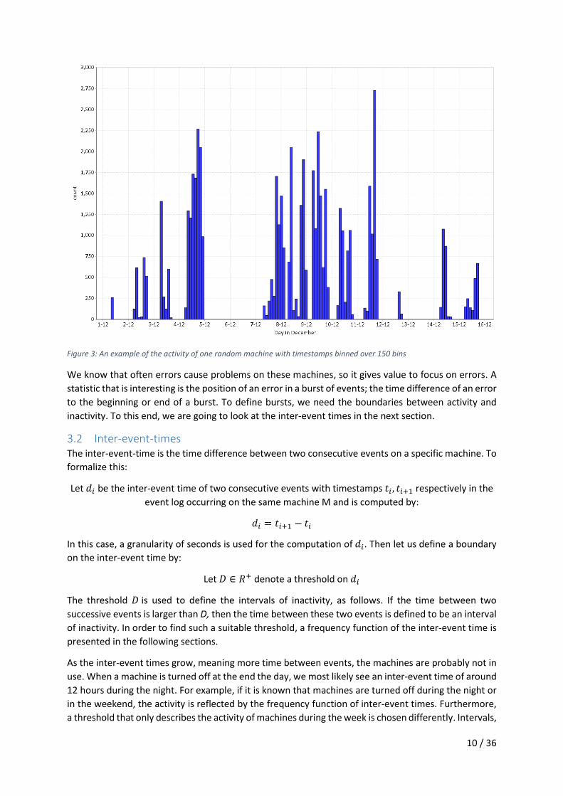
3.1 Activity of machines An example of the activity for a randomly chosen is illustrated in Figure 3. This example is typical for

the selection of machines chosen during the process of this study.

In Figure 3 the number of events on a timestamp with a certain event category is depicted, we call this

the Event frequency. We bin timestamps from 1 December 2015 to and including 15 December and

count the number of events per bin, here 150 bins are chosen. It is clear to see that there are intervals

with events and intervals without events. This suggests that machines are either shutdown by human

interaction or crashed due to events occurring just before the shutdown.

Attributes such as the number of events per day can be skewed by these intervals of inactivity. As an

example, not related to Figure 3, let us assume a machine that only produces events when it is on. This

machine is on during work days and is off over the weekend. The average number of events per day

would then be the sum of the number of events divided by seven. However, to truly represent the

average number of events, the average should be larger (thus divided by five), as the machine is only

on during working days. To truly represent these attributes we are going to only look at the intervals

having events. These intervals will later be called bursts and will be later defined in Section 3.2.2.

10 / 36

Figure 3: An example of the activity of one random machine with timestamps binned over 150 bins

We know that often errors cause problems on these machines, so it gives value to focus on errors. A

statistic that is interesting is the position of an error in a burst of events; the time difference of an error

to the beginning or end of a burst. To define bursts, we need the boundaries between activity and

inactivity. To this end, we are going to look at the inter-event times in the next section.

3.2 Inter-event-times The inter-event-time is the time difference between two consecutive events on a specific machine. To

formalize this:

Let 𝑑𝑖 be the inter-event time of two consecutive events with timestamps 𝑡𝑖 , 𝑡𝑖+1 respectively in the

event log occurring on the same machine M and is computed by:

𝑑𝑖 = 𝑡𝑖+1 − 𝑡𝑖

In this case, a granularity of seconds is used for the computation of 𝑑𝑖. Then let us define a boundary

on the inter-event time by:

Let 𝐷 ∈ 𝑅+ denote a threshold on 𝑑𝑖

The threshold 𝐷 is used to define the intervals of inactivity, as follows. If the time between two

successive events is larger than D, then the time between these two events is defined to be an interval

of inactivity. In order to find such a suitable threshold, a frequency function of the inter-event time is

presented in the following sections.

As the inter-event times grow, meaning more time between events, the machines are probably not in

use. When a machine is turned off at the end the day, we most likely see an inter-event time of around

12 hours during the night. For example, if it is known that machines are turned off during the night or

in the weekend, the activity is reflected by the frequency function of inter-event times. Furthermore,

a threshold that only describes the activity of machines during the week is chosen differently. Intervals,

11 / 36

which reflect the usage of the machines with interval lengths of a day, a week or longer, are then

created. In order to find a period in which a machine is inactive, we look at the frequency function of

the inter-event time.

The frequency function 𝑓𝑟𝑒𝑞𝑢𝑒𝑛𝑐𝑦(𝑑𝑖) on the domain over all values of 𝑑𝑖 is defined as the number

of occurrences of 𝑑𝑖 in the dataset.

An example on the dataset of December 2015 is found in Figure 4. As the frequency in the first twenty

minutes is rather large in comparison to the rest of the data it is omitted in Figure 4.

To find a suitable value for 𝐷 we are going to use some domain knowledge in combination with the

histogram in Figure 4. We would like to know when a system is turned off, not by human input, but by

errors shutting down the system, as it indicates the anomalous behavior of the machine. As we will see

in the next subsections, some parts of the frequency graph in Figure 4 can be explained by using

domain knowledge. The inter-event-times that cannot be explained by domain knowledge are

assumed to be shutdowns without human intervention.

3.2.1 Inter-event-time In Figure 4, a histogram of 𝑑𝑖 is found, limited by 𝑑𝑖 = 72 hours for clarity. The upper bound is

chosen as we assume that inter-event times greater than 72 hours does not give us more information

than inter-event times smaller than 72 hours.

Figure 4: Histogram of 𝑑𝑖 ≤ 72 hours with indication of peaks.

Each of the peaks in Figure 4 represents specific scenarios. The first red region from the left describes

a shutdown during the day and a startup the next morning. The third red region indicates a shutdown

during the day, a full day and a startup in the morning after that full day. The fourth red region

illustrates a shutdown during the last day before the weekend, a weekend and a startup on the

morning after a weekend.

12 / 36

One red region does not fall into the same category as the others. The second red region consists of a

shutdown in the morning and a startup in the following morning. To illustrate this further, we look at

the timestamps 𝑡𝑖 of the events with 𝑑𝑖~24, which is depicted in Figure 5. Figure 5 confirms that a

shutdown primarily happens between 6 and 10 AM.

Figure 5: 𝑡𝑖 of events in hour of day with 𝑑𝑖 ~ 24

With the assumption that inter-event times smaller than two hours are most likely explained by breaks

by the hospital personnel or the inactivity between patients, we deduce an interval of values that are

suitable as value for 𝐷. Also we would like a value for 𝐷, which is smaller than ~14 hours, to exclude

regular shutdowns. When more information is known about the inter-event times or the regular

shutdowns of the system it is possible to adapt the choice to include that information. Based on the

data illustrated in Figure 4 and the assumptions, the interval indicated by a green rectangle in Figure 4

represent the suitable values 3 ≤ 𝐷 ≤ 8. In the remainder of this thesis, a value of six hours is chosen

as threshold 𝐷.

3.2.2 Definitions bursts and sequence of bursts Using the investigation of the inter-event times we define the activity of machines. In that way, we

define statistics relative to the time that a machine was in use instead of the traditional statistics (e.g.

the number of events per second). Let us formalize these intervals as bursts:

A burst is an interval of timestamps of events occurring on machine M in the event log.

It is denoted by [𝑡𝑏 , … , 𝑡𝑒], with 0 ≤ 𝑏 ≤ 𝑒 ≤ 𝑁, where, for each 𝑘, 𝑤𝑖𝑡ℎ 𝑏 ≤ 𝑘 < 𝑒, it holds

that 𝑡𝑘+1 − 𝑡𝑘 ≤ 𝐷.

Let the ordered sequence of bursts be given by 𝐵0, 𝐵1, … , 𝐵𝑚−1, which, together, cover all

timestamps of log events of machine M.

Figure 6 shows an example of bursts 𝐵𝑖 on three machines 𝑀1, 𝑀2 and 𝑀3. For each machine 𝑡𝑏 , 𝑡𝑒

are created, however subscripts are omitted in Figure 6 for readability purposes.

13 / 36

Figure 6: Example of bursts for three machines

This definition of a burst enables us to represent the activity of machines such that it is possible to

form statistics over the events occurring within these bursts. This also concluded the first step of the

algorithm. In the next section, we present the enrichment of the data by creating attributes such as

the positions of errors within its respective bursts and the length of the burst.

Figure 7: Overview of the algorithm, with completed steps highlighted

Data extraction


Data enrichment


Data aggregation

(vector creation)



Outlier

detection


14 / 36

4. Statistics of bursts In order to define vectors for the clustering algorithm presented in the next section, we first use the

definition of a burst to find the start- and end-timestamps on the dataset for December 2015. As the

implementation in RapidMiner uses a tuple based dataset and we focus on events with category error.

We create an instance of the burst for each error e, which means that each burst instance (tuple) of

error e consists of the following attributes (some we have seen before):

Attributes Comment

SRN Serial number of a machine; identifies a specific machine

Equipmentnumber Equipment number of a machine; identifies a specific machine

EventId Event identification

EventTimestamp Timestamp of recorded event

Description Description of the event

EventCategory Type of event. [Error, Warning, Command, UserMessage, Information]

AdditionalInfo Provides more information into the event

Software release Software Release of the software on the machine

SystemCode Specifies the type of system

𝒕(𝒆) Timestamp of the event 𝑒, with EventCategory Error

𝒕𝒃 Timestamp of the beginning of the burst

𝒕𝒆 Timestamp of the end of the burst

𝒏𝒆𝒙𝒕 Time to the next burst

𝒑 The position of the error in the burst

𝒒 The position of the error in the burst with respect to the end of the burst

𝑳 Length of the burst

𝒏𝒐𝒓𝒎(𝒑) Position of the error in the burst with respect to the length of the burst

Note: some are omitted in the following datasets, but were included for data exploration purposes.

4.1 Calculation of begin and end of a burst. In order to create the attributes and aggregated values, we first determine the begin- and end-

timestamps of the bursts. These timestamps are computed by filtering the iXR event log on the 𝑑𝑖

calculated before. Note that the following paragraphs are highly dependent on the implementation,

here we explain the transformation from tuples of consecutive events to boundaries of the bursts.

An event has the following attributes:

𝑒 = 𝑆𝑅𝑁|𝐸𝑞𝑢𝑖𝑝𝑚𝑒𝑛𝑡𝑛𝑢𝑚𝑏𝑒𝑟|𝑡𝑖|𝑡𝑖+1|𝑡0|𝐸𝑣𝑒𝑛𝑡𝐶𝑎𝑡𝑒𝑔𝑜𝑟𝑦|𝐸𝑣𝑒𝑛𝑡𝐼𝑑

Suppose we have two consecutive events in the event log on the same machine 𝑀. The event-

timestamp for event 𝑒 is 𝑡𝑖. The event timestamp for the next consecutive event is 𝑡𝑖+1. A small

simplified example is illustrated in Table 1. Note that the time is omitted for readability, but is

present in the data.

15 / 36

Table 1: example of the leading attributes

𝒕𝒊 𝒕𝒊+𝟏

1-12-2015 2-12-2015 2-12-2015 3-12-2015 3-12-2015 4-12-2015 4-12-2015 5-12-2015 5-12-2015 ?

Given 𝑡𝑖 and 𝑡𝑖+1 the calculation of 𝑑𝑖 is straightforward. Then the dataset is filtered on the

threshold 𝑑𝑖 ≥ 𝐷, which results in a dataset consisting of instances of burst boundaries having

timestamps before and after the inactivity of a machine. However, that is the inverse of what actually

is needed. The boundaries are found by defining the end timestamp at the beginning of the “gap”,

depicted by the red arrows in Figure 8 and defining the beginning of the next burst to the end of the

“gap”, thus 𝑡𝑒 = 𝑡𝑖.

The calculation of 𝑡𝑏 is somewhat more complicated. The timestamp after the “gap” of inactivity

becomes 𝑡𝑏, which is illustrated in the table below.

In contrast to the missing value of Table 1 in Table 2 the missing value is one of the boundaries of a

burst in the dataset. In Table 1, 5 December 2015 was the end-timestamp of the last burst in the

example in Table 2. However, the missing value in Table 2 is, in fact, the begin-timestamp of the first

burst in this example, thus, it is needed. The missing value in Table 2 is found by the applying the

value of 𝑡0 we have seen before.

Table 2: example of lagging attributes

𝒕𝒊+𝟏 𝒕𝒃

1-12-2015 ? 2-12-2015 1-12-2015 3-12-2015 2-12-2015 4-12-2015 3-12-2015 5-12-2015 4-12-2015

Figure 8: illustration of the boundary and burst creation

𝑑𝑖 ≥ 𝐷 𝑑𝑖 ≥ 𝐷

𝑑𝑖 ≥ 𝐷

𝑡𝑖 → 𝑡𝑒 𝑡𝑖+1 → 𝑡𝑏 𝑡𝑒

𝑑𝑖 ≥ 𝐷 𝑑𝑖 ≥ 𝐷

16 / 36

In summary, from the raw event log the begin- and end-timestamps of the burst are calculated by

manipulating the event-timestamps by means of leading and lagging in order to create a tuple defining

a burst 𝑏𝑖:

𝑏𝑖 = 𝑆𝑅𝑁|𝐸𝑞𝑢𝑖𝑝𝑚𝑒𝑛𝑡𝑛𝑢𝑚𝑏𝑒𝑟|𝑡𝑏|𝑡𝑒|𝐸𝑖

with 𝐸𝑖 the set of 𝐽 events within that burst and defined by:

𝐸𝑖 = (𝑒𝑖,1, 𝑒𝑖,2, . . , 𝑒𝑖,𝑗, . . , 𝑒𝑖,𝐽)

Thus, the event log has a set of bursts, divided over several machines, with each machine having

𝐼 bursts. It is defined by:

𝐵 = (𝑏1, . . , 𝑏𝑖, . . , 𝑏𝐼)

4.1.1 Burst length The length of the burst is easily calculated with these boundaries. The length of a burst is simply the

end-timestamp minus the begin-timestamp or

𝐿(𝑏𝑖) = 𝑡𝑒(𝑏𝑖) − 𝑡𝑏(𝑏𝑖) with 𝑏𝑖 ∈ 𝐵

The distribution of the length of all bursts over December 2015 is illustrated in Figure 9, with the length

on the x-axis and the frequency on the y-axis.

Figure 9: Length of bursts in December 2015

It is clear that several different types of bursts are distinguished. There are a large number of bursts

with lengths up to ~12 hours and decreasing to around ~100 hours. Furthermore, it is interesting that

two peaks at 150 and 360 hours stand out. When we zoom in at bursts that end within a day (24 hours)

more interesting observations are seen. For example, it is most likely that bursts end within the hour

or after a typical working day of eight hours. As seen in Figure 10.

17 / 36

Figure 10: Length of burst that end within 24 hours.

4.2 Position of error An attribute used in the clustering algorithm is the relative position of an error in a burst. In this case,

three of these metrics are described:

1. Position with respect to the beginning of the burst, in which it occurs.

2. Position with respect to the end of the burst, in which it occurs.

3. Position with respect to the length and the beginning of the burst, in which it occurs.

Each of these is calculated by manipulating the timestamps of the error and begin- and end-

timestamps of the corresponding burst.

4.2.1 Position with respect to the beginning of the burst In burst 𝑏𝑖 the position of an error 𝑒𝑖,𝑗, with respect to the beginning of the burst is calculated by

computing the difference between the timestamp of the error and the begin-timestamp of the burst

or

𝑝𝑗(𝑏𝑖) = 𝑡(𝑒𝑖,𝑗) − 𝑡𝑏(𝑏𝑖) with 𝑏𝑖 ∈ 𝐵

As we have seen in Figure 9 it is most likely that bursts end within 24 hours. Therefore, the position of

an error within the burst will most likely also be within 24 hours. Therefore, we are going to look at

the position of the errors that occurs within 24 hours of the beginning of the burst. The result of the

dataset of bursts over December 2015 𝑝𝑗 is illustrated in Figure 11. As seen the position of the error

within the burst is most likely to be within the first hour or at around 5 hours. However, as the number

of bursts decreases when 𝐿 increases, we only conclude there are more bursts with position at around

18 / 36

5 hours than 17 hours. In Section 4.2.3 this alleviated by dividing 𝑝 by the burst length, normalizing the

bursts to the same lengths.

Figure 11: Position of errors within 24 hours of the beginning of the burst.

4.2.2 Position with respect to the end of the burst In burst 𝑏𝑖 the position of an event 𝑒𝑖,𝑗, with event category error, with respect to the end of the burst

is calculated by computing the difference between the timestamp of the error and the end-timestamp

of the burst or

𝑞𝑗(𝑏𝑖) = 𝑡𝑒(𝑏𝑖) − 𝑡(𝑒𝑖,𝑗) with 𝑏𝑖 ∈ 𝐵 and 𝑒𝑖,𝑗 ∈ 𝐸𝑖

4.2.3 Position with respect to the length and the beginning of the burst The position of an error with respect to the length and beginning of the burst is calculated by

computing the difference between the timestamp of the error and the begin-timestamp of the burst

and dividing that by the length of the burst or:

𝑛𝑜𝑟𝑚(𝑝𝑗) = 𝑝𝑗/𝐿

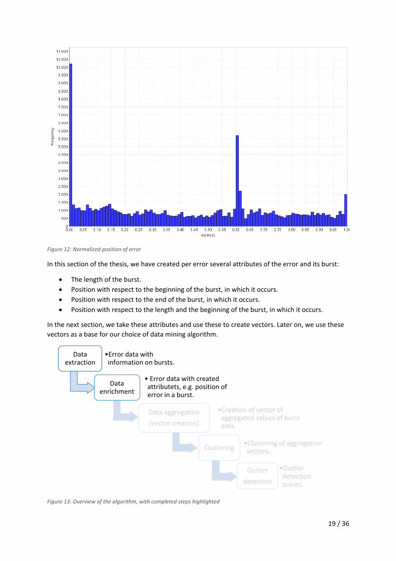
In the dataset of bursts over December 2015 𝑛𝑜𝑟𝑚(𝑝𝑗) is illustrated in Figure 12. Interesting to see

that it is most likely that errors occur at the beginning, at 61% of the burst length or at the ending of

its’ respective burst. Later, this will most likely be used by the clustering algorithm to classify different

clusters based on this attribute. For example, it is likely that bursts with a low 𝑛𝑜𝑟𝑚(𝑝𝑗) will be placed

in other clusters than bursts with a high 𝑛𝑜𝑟𝑚(𝑝𝑗). Similarly, bursts with errors on 61% of its length

will be placed in another cluster.

19 / 36

Figure 12: Normalized position of error

In this section of the thesis, we have created per error several attributes of the error and its burst:

The length of the burst.

Position with respect to the beginning of the burst, in which it occurs.

Position with respect to the end of the burst, in which it occurs.

Position with respect to the length and the beginning of the burst, in which it occurs.

In the next section, we take these attributes and use these to create vectors. Later on, we use these

vectors as a base for our choice of data mining algorithm.


Data extraction


Data enrichment


Data aggregation

(vector creation)



Outlier

detection


20 / 36

5. Aggregated values over bursts Using the statistics per burst we have created in the previous section, we define a vector by averaging

the attributes defined before. A lot of aggregation techniques can be applied to create statistics over

the bursts, from simply counting the number of errors to some more complicated aggregation as

standardization of the attributes. In this case, the average values of the attributes are chosen, which

could easily be enhanced with the standard deviation to create a clearer overview of the statistics over

a burst.

These attributes are created by aggregating over the burst and averaging the values, which is easily

done by any datamining software package. Furthermore, the number of errors and the number of

errors by prefix are added. These will be explained in a later section of this chapter.

For each burst 𝑏𝑖 let us define a vector 𝑉𝑖:

𝑉𝑖 = (𝑡𝑏(𝑏𝑖), 𝑡𝑒(𝑏𝑖), 𝐿(𝑏𝑖), �̅�, �̅�, 𝑛𝑜𝑟𝑚(𝑝𝐽)̅̅ ̅̅ ̅̅ ̅̅ ̅̅ ̅̅ ̅, |𝐸𝑖|, 𝑐𝑎,𝑏(𝑏𝑖) )

5.1 Number of errors per burst The number of errors per burst is calculated by:

|𝐸𝑖| = ∑ 1

𝑒𝑖,𝑗∈𝐸𝑖

Also the number of errors with unique EventIds can be computed in a similar manner, but is here

omitted.

5.2 Average position with respect to the beginning of the burst. The fourth attribute of the vector used in the clustering algorithm is the average position of an error

with respect to the beginning of the burst. The average position is calculated by summing every 𝑝𝑥 per

burst or:

�̅� = ∑ 𝑝𝑗(𝑏𝑖)


/ |𝐸𝑖|

5.3 Average position with respect to the end of the burst. The fifth attribute of the vector used in the clustering algorithm is the average position of an error with

respect to the end of the burst. The average position is calculated by summing every 𝑞𝑥 per burst or:

�̅� = ∑ 𝑞𝑗(𝑏𝑖)


/ |𝐸𝑖|

5.4 Average position with respect to the length and the beginning of the burst. The sixth attribute of the vector used in the clustering algorithm is the average position of an error

with respect to the beginning of the burst. The normalized average position is calculated by summing

every 𝑛𝑜𝑟𝑚(𝑝𝑗) per burst or:

𝑛𝑜𝑟𝑚(𝑝𝑗)̅̅ ̅̅ ̅̅ ̅̅ ̅̅ ̅̅ ̅ = ∑ 𝑛𝑜𝑟𝑚(𝑝𝑗)


/ |𝐸𝑖|

21 / 36

5.5 Number of errors per burst per prefix In order to find a relationship of a burst to the errors occurring in that burst we look at the eventIds.

From domain knowledge, we know that the first two digits of said eventId are both directly or indirectly

related to the component of a subsystem of the iXR-machine which sends the event. Therefore, it is

interesting to include the statistics.

As we are going to look at 2 digits, say 𝑎 and 𝑏, with 𝑎, 𝑏 ∈ 0. .9, there are at most 10 ∗ 10 = 100

possible combinations. In the dataset, only 35 combinations occur. Per combination of 𝑎 and 𝑏, we will

count the number of events having that combination and is also called the prefix of the eventId.

Let 𝑐𝑎,𝑏(𝑒𝑖,𝑗) = {1 if 𝑒𝑣𝑒𝑛𝑡𝐼𝑑(𝑒𝑖,𝑗) start with 𝑎 and 𝑏

0 Otherwise}

So for any combination of 𝑎 and 𝑏 we have:

𝑐𝑎,𝑏(𝑏𝑖) = ∑ 𝑐𝑎,𝑏(𝑒𝑖,𝑗)


To conclude this section, first let us repeat the first research question of this thesis:

How can event data from iXR-machines be represented?

In Sections 3 and 4 and this section, we have seen that an event log from an ISDA-database is

represented in a more descriptive way. Using the definitions in Section 5, we created vectors with

aggregated values that describe each burst. These sections thus answer the first research question.

Furthermore, these vectors are used in the next section to compare bursts by means of a clustering

algorithm.


Data extraction


Data enrichment


Data aggregation

(vector creation)



Outlier

detection


22 / 36

6. Clustering on vectors Using the definition of the vector of attributes we compare these vectors with some standard data-

mining algorithms. As we do not have labels at our disposal we are situated in an unsupervised setting.

As we have seen before in Section 2.2 there are several algorithms of different types available to us.

The first type to consider is the nearest neighbor based algorithms. These algorithms assume that

anomalies occur far from their closest neighbors. One of the key advantages is that nearest neighbor

algorithm does not make any assumptions regarding the generative distribution of the data; they are

purely data driven. As these algorithms evaluate each data instance with respect to its’ local

neighborhood instead of its’ cluster, it seems that a choice for these algorithms is not founded.

However, as we will see later on the choice of a k-means algorithm is loosely based on nearest neighbor

techniques.

The second type of algorithms that are considered are the clustering based algorithms. As seen before

in Section 2.2.2 there are three main assumptions that differentiate the clustering based algorithms.

We expect that vectors of similar bursts will be closely clustered to each other as similar machines

most likely behave in the same manner. Therefore, we would like to know what the anomalies within

each cluster are. It is, however, possible that small or sparse clusters describe anomalies. Under these

considerations, the choice of a k-means algorithm is made.

6.1 Clustering algorithm overview K-means clustering is a method of vector quantization, which is popular for cluster analysis in data

mining [13]. K-means clustering aims to partition n observations into k clusters in which each

observation belongs to the cluster with the nearest mean, serving as a prototype of the cluster, also

referred to as the centroid of the cluster.

Given a set of observations (𝑥1, 𝑥2, … , 𝑥𝑛) where each observation is a d-dimensional vector, k-means

clustering aims to partition the 𝑛 observations into 𝑘 (≤ 𝑛) sets 𝑆 = {𝑆1, 𝑆2, … , 𝑆𝑘} so as to minimize

the within-cluster sum of squares (WCSS) (sum of distance of each point in the cluster to the centroid)

[14].

6.2 Normalization of the data In order to create a sound distance measure the attributes must compare mathematically to each

other. For example, a large difference between the large lengths and small 𝑛𝑜𝑟𝑚(𝑝)̅̅ ̅̅ ̅̅ ̅̅ ̅̅ ̅̅ values can skew

the evaluation as the large values of the length attribute is weighted higher than other attributes.

Therefore, it is often sound to normalize the data and is done with several methods:

Z-transformation/Standard score: for each attribute value subtract the mean value of that

attribute and dividing the result by the standard deviation of that attribute [15].

Range-transformation: Setting the range of an attribute to the range minimum and maximum.

If these are the same throughout the attributes range-transformation will normalize all

attributes.

Proportion-transformation: Each attribute is normalized as the proportion of the total sum of

that attribute. In other words, each attribute value is divided by the total sum of that attribute

value.

Interquartile range: As range transformation is heavily influenced by outliers in the data, the

interquartile range is used as a criterion. The interquartile range is the distance between the

25th and 75th percentiles. Effectively, the interquartile range uses the middle 50% of the range

of the attribute and thus is not affected by outliers or extreme values.

23 / 36

6.3 Distance Measure Initially, k-means clustering is only applied on vectors with vectors with real values. However, as our

data do not only contain attributes with real values, but also uses the begin- and end-timestamp of the

burst, the traditional Euclidean distance cannot (directly) be used. However, the implementation uses

a mixed measure approach: for real values the Euclidean distance is used, for nominal values the

distance is 1 if both values are not the same and 0 otherwise.

6.4 Number of clusters One of the disadvantages of using the 𝑘-means algorithm is that the number of clusters needs to be

given as a parameter before the execution of the algorithm. In order to find 𝑘, first let us focus on the

predictability of the clustering. The cluster labels are predicted by a 10-fold validation using a decision

tree and compared to the clustering computed by 𝑘-means. Note that any prediction algorithm can be

used in one fold, but a decision tree is chosen as one advantage of a decision tree is that it visualizes

the choices made by the algorithm.

6.4.1 10-fold validation using a decision tree The set with cluster labels is used as input for the 10-fold validation, which in 10 rounds splits the data

in 10 different training and test/validation sets. The performance of the prediction of the cluster-label

by a decision tree is aggregated over these 10 rounds. An example is found in Figure 15.

.

Figure 15: 10 fold validation example

Let us view the 10-fold validation in more detail by explaining one fold of 10-fold validation. In this

case, a decision tree is used to predict the cluster labels of a 10th of the data. A training set containing

cluster labels and its’ size is 90% of the data on which a decision tree model is learned. The parameters

used by a decision tree prediction algorithm highly depends on the number of attributes and the

information gained by choices during the algorithm. Also, the accuracy of the prediction changes when,

for example, the maximum depth of the tree increases. An example of a 6-depth decision tree is found

in Figure 16. In most cases a maximum depth of 10 is used to ensure a high accuracy.

24 / 36

Figure 16: Example of 6-depth decision tree

In Table 3 the prediction accuracy per choice of 𝑘 is found. The accuracy does not differ that much

from 2 to 10 clusters. Therefore, the number of clusters is chosen arbitrarily in terms of accuracy, so

further analysis is required.

Table 3: 10-fold accuracy per number of clusters

NUMBER OF CLUSTERS ACCURACY IN %

2 98.55 3 98.92 4 98.85 5 99.17 6 98.49 7 94.41 8 80.83 9 75.64 10 77.50

An example of the visualization, mentioned in the beginning of this section is found in Figure 16, is also used to explore the characteristics. However, it is not used in the anomaly detection algorithm other than for validation or exploration purposes.

6.4.2 Average distances to centroid A second method to find the number of clusters is to find the average distance to the centroid of that

cluster. As k-means uses a similar measure to base its decision of what cluster the instance is appointed

25 / 36

to, this measure is of great value. For each point, the distance to its’ respective cluster is calculated

and is averaged over all point, which gives the average intra-cluster or within cluster distance. The

average within cluster distances is used to give a value to the ‘performance’ of that choice of 𝑘. The

‘best’ choice for 𝑘 is where the average distance to the centroid is lowest. An overview is found in

Table 4.

Table 4: average distance per number of clusters.

NUMBER OF CLUSTERS

AVERAGE WITHIN CLUSTER DISTANCE

AVERAGE BETWEEN CLUSTER DISTANCE

MEDIAN BETWEEN CLUSTER DISTANCE

RATIO

2 2.8673 2.9674 2.9674 0.9663 3 2.5751 2.7704 2.2408 0.9295 4 2.4651 2.5838 1.8853 0.9541 5 2.2706 2.7728 2.7451 0.8189 6 2.1535 2.9075 2.7354 0.7407 7 2.1747 2.9254 2.8685 0.7434 8 2.1413 3.1918 3.1750 0.6709 9 2.0223 3.3242 3.1945 0.6084 10 2.0501 12.3843 3.5970 0.1655 11 1.9680 3.2791 3.2588 0.6002 12 1.9028 10.8432 3.6173 0.1755 13 1.9506 10.2108 3.1806 0.1910 14 1.8517 9.9074 3.7298 0.1869 15 1.7188 3.3460 3.1455 0.5137 16 1.8546 3.3201 3.0965 0.5586 17 1.6942 11.1020 3.8770 0.1526 18 1.6886 8.5088 3.7603 0.1985 19 1.6692 10.5471 4.0450 0.1583 20 1.6437 7.7360 3.1516 0.2125

The result in the second column of Table 4 can be enhanced by not only taking the intra-cluster

distances in consideration but also the distances between the clusters. A good clustering has a low

intra-cluster distance and a high inter-cluster or between cluster distance. Several measures are often

applied to find a suitable value of the parameter 𝑘 depending on these distances. One used here is the

ratio of average intra-cluster distance divided by the inter-cluster distance. Given that a clustering

algorithm works well if the intra-cluster distance is low and the inter-cluster distance is high, the ratio

is small. Given this, two possible solutions are indicated by bold font in Table 4. The choice of number

of clusters is not only dependent on observations we have seen earlier but also the performance of 𝑘-

means on a laptop. Although the optimal solution of 𝑘 is 17, we decided for 𝑘 = 10 as this results in a

less complex model and has comparable performance in terms of result to 𝑘 = 17.

6.5 Result of clustering Using the choice of 𝑘 we continue with the application of 𝑘-means on the dataset of December 2015.

To reiterate, we have created vectors with aggregated attribute values describing burst. These

vectors are clustered by 𝑘-means. As the vectors are let us say 𝑛 attributes long, the clustering is

done in a 𝑛-dimensions, which makes visualizing the clustering fairly difficult. To overcome this

problem we use Principal Component Analysis (PCA) [16] to find the attributes that are most

important and more highly weighted by 𝑘-means. In this case, the combination of the average length

26 / 36

of the burst and the average position of the error within its burst is most important. A scatterplot

with these attributes on the axes is found in Figure 17. Three clusters with large average lengths are

easily distinguished, to explore the rest of the cluster we will zoom in onto the left-bottom corner,

indicated by a red rectangle. The result is found in Figure 18 where three more clusters are

distinguished.

Figure 17: Scatterplot of clustering

Figure 18: Zoomed scatterplot

27 / 36

Lastly, let us look at the sizes and averages of the two most important attributes of the vectors of the

clusters, which are found in Table 5. Note that the average length and average position of the errors

are normalized thus cannot be directly used and can be negative. However, the differences between

clusters are on par with the non-normalized data. The clusters are very different, some are a lot

bigger than others. Furthermore, a big difference in attributes is seen.

Table 5: Size, average length and average position of error per cluster

Cluster Size Average Length

Average Position of error

cluster_0 7061 -0.195 -0.267

cluster_1 4402 -0.170 0.002

cluster_2 1449 -0.173 -0.154

cluster_3 45 0.249 0.317

cluster_4 3251 1.367 0.972

cluster_5 20392 -0.134 -0.059

cluster_6 10481 -0.100 0.192

cluster_7 26439 -0.164 -0.274

cluster_8 681 5.333 4.435

cluster_9 153 15.798 15.308

In this section, we have discussed how the data is normalized, what distance measure is used and

how many clusters is needed for 𝑘-means. Using 𝑘-means we have seen that there are both

similarities and dissimilarities between the clusters. Therefore, we have presented a way to identify

(dis)similarities between bursts of events answering the second research question:

How can we identify similarities between bursts of events?

In the next section, this clustering is used to apply several outlier factor algorithm to produce a

ranking of bursts, the last step of the anomaly detection algorithm.


Data extraction


Data enrichment


Data aggregation

(vector creation)



Outlier

detection


28 / 36

7. Outlier detection The clustering algorithm explained in the previous section added a label to the dataset and will be used

to find outliers. Examples of the many outlier detection algorithms that are applicable are:

Cluster based Local Outlier Factor (CBLOF)

Local Density Cluster based Outlier Factor (LDCOF)

Clustering based Multivariate Gaussian Outlier Score (CMGOS)

The first and second algorithms are used in the anomaly detection algorithm explained in the thesis.

The latter is omitted in that algorithm as it created performance issues in the implementation. It is,

however, included as a reference.

7.1 Cluster based Local Outlier Factor (CBLOF) As we have seen before, the cluster based local outlier factor is defined as:


𝐶𝐵𝐿𝑂𝐹(𝑡) = |𝐶𝑖 | ∗ 𝑚𝑖𝑛𝐶𝑗∈𝐿𝐶 (𝑑(𝑡, 𝐶𝑗))


𝐶𝐵𝐿𝑂𝐹(𝑡) = |𝐶𝑖 | ∗ (𝑑(𝑡, 𝐶𝑖))

CBLOF takes as an input the data set and the cluster model that was generated by 𝑘-means. It

categorizes the clusters into small and large clusters using the default parameters 𝛼 = 90 and 𝛽 = 5.

The anomaly score is then calculated based on the size of the cluster the point belongs to as well as

the distance to the nearest large cluster centroid.

It uses weighting for CBLOF based on the sizes of the clusters as proposed in the original publication

[17]. Weighting might lead to unexpected behavior as outliers close to small clusters are not found

[18]. It can be disabled and outliers’ scores are solely computed based on their distance to the cluster

center. In this case, we decided to enable the weighting as we expect that the sizes of the clusters are

of importance.

When we apply this to the dataset we see interesting observations. For example, the CBLOF score for

bursts from the “smaller” clusters is significantly lower than the “bigger” clusters. Statistics of the

average ranking is found in Table 6. It is clear to see that the average CBLOF score differs greatly

between clusters.

7.2 Local Density Cluster based Outlier Factor (LDCOF) As we have seen before, the local density cluster based outlier factor with is defined as:


𝐿𝐷𝐶𝑂𝐹(𝑡) =min

𝐶𝑖∈𝐿𝐶(𝑑(𝑡, 𝐶𝑗))

𝑑𝑎𝑣𝑔(𝐶𝑗)


𝐿𝐷𝐶𝑂𝐹(𝑡) =𝑑(𝑡, 𝐶𝑖)

𝑑𝑎𝑣𝑔(𝐶𝑖)

29 / 36

with an average distance for points within a cluster 𝐶 as:

𝑑𝑎𝑣𝑔(𝐶) =∑ 𝑑(𝑡, 𝐶)𝑡 ∈𝐶

|𝐶|

The anomaly score is set to the distance to the nearest large cluster divided by the average cluster

distance of the large cluster. The intuition is that the small clusters are considered outlying and thus

they are assigned to the nearest large cluster and this becomes its local neighborhood.

The division into large and small clusters can be either done similar to what was implemented in the

CBLOF algorithm or it is done in a manner similar to what was proposed in [17].

Statistics for the LDCOF score are found in Table 6. As with the CBLOF score, the LDCOF algorithm

produces a big difference in scores per cluster. An interesting observation is that the average LDCOF

score of cluster_3 and cluster_9 is very high with respect to the other clusters, indicating that these

clusters contains outliers.

Table 6: Statistics of CBLOF ranking per cluster

Cluster Size Average CBLOF score

Std CBLOF score

Average LDCOF score

Std LDCOF score

cluster_0 7061 5533.91 3048.89 1.00 0.55

cluster_1 4402 4153.41 3202.35 1.00 0.77

cluster_2 1449 4851.91 3549.95 1.00 1.11

cluster_3 45 2124.53 1771.32 46.70 36.23

cluster_4 3251 9395.92 8254.18 1.00 1.26

cluster_5 20392 11829.89 15057.94 1.00 1.27

cluster_6 10481 8805.38 14736.79 1.00 1.67

cluster_7 26439 13001.56 14458.06 1.00 1.11

cluster_8 681 7089.95 5815.92 4.32 4.50

cluster_9 153 4225.12 1144.38 13.13 3.90

In this section, we have applied the definitions from Sections 2.3 and 2.4 to create a ranking of bursts

based on the CBLOF and LDCOF score algorithms. We have seen that big difference between clusters

exist in both scores and that cluster_3 contains outlying bursts. The third research question of this

thesis is:

How can machines be ranked using the properties of sets of bursts?

With this section, this research question is answered as machines are now ranked using the CBLOF

and LDCOF scores. Furthermore, these scores have indicated that there is a difference between the

clusters. This also concludes the last part of the anomaly detection algorithm. In the next section, we

are going to relate this ranking to the call data provided by Philips.

30 / 36


Data extraction


Data enrichment


Data aggregation

(vector creation)



Outlier

detection


31 / 36

8. Validation by relating call data to clustering In order to validate both the CBLOF as the LDCOF ranking, we relate the rankings to call data provided

by Philips. Furthermore, we will use the call data to find differences between the clusters.

Call data consists of the following attributes depicted in Table 7 and describe the requests for

maintenance made by the hospital to the service center. The call data originates from a different setup

than the event log of the ISDA database, thus has different attributes than the event log. However, the

combination ConfigID/ConfigSerialNr is the same as the Equipmentnumber/SRN combination

respectively.

Table 7: Call data attributes

Attribute Comment

CountryName Country from which the call originated

ConfigID Same as Equipmentnumber

ConfigSerialNr Same as SRN

CallID Identification of the call

CallOpenDate Data on which the call is opened

Description Information about the problem

12NC Code to identify the type of problem

First we will look at the relation of the call data to the clustering. Let us define call bursts as:

The number of bursts that result in a call

A burst results in a call when the CallOpenDate of a call is after the end of the burst and the

call occurs on the same machine as the burst, obviously.

Only the first call is taken into account when there are multiple calls after a burst.

We compute the average time from the end of a burst (𝑡𝑒) to the date on which a call is opened. Let

us define 𝑡𝑖𝑚𝑒𝑇𝑜𝐶𝑎𝑙𝑙(𝑏𝑖) where 𝑏𝑖 is a burst in cluster 𝐶𝑗 ∈ 𝐶 as the time of that burst to the first

call or more formally:

𝑡𝑖𝑚𝑒𝑇𝑜𝐶𝑎𝑙𝑙(𝑏𝑖) = 𝐶𝑎𝑙𝑙𝑂𝑝𝑒𝑛𝐷𝑎𝑡𝑒 − 𝑡𝑒(𝑏𝑖)

The arrows in Figure 21 gives three examples of the time from a burst to a call. The blue rectangles

represent bursts, the red rectangles represents calls. Note that the second red rectangle does not

have incoming arrows.

The values represented by the arrows are then averaged over the bursts per cluster. These average

values are found in Table 8. These average values tells us some interesting relations between the

average time to call and the cluster. For example, the average time to a call for cluster_3 is significantly

lower. As we have seen before cluster_3 also had a high average LDCOF score. So it becomes clearer

Figure 21: Time to call example

𝑡𝑖𝑚𝑒𝑇𝑜𝐶𝑎𝑙𝑙(𝑏1)

32 / 36

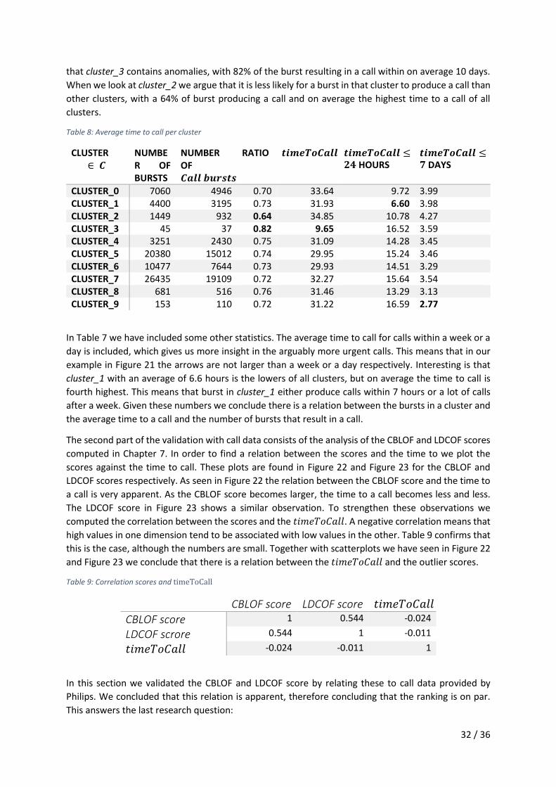
that cluster_3 contains anomalies, with 82% of the burst resulting in a call within on average 10 days.

When we look at cluster_2 we argue that it is less likely for a burst in that cluster to produce a call than

other clusters, with a 64% of burst producing a call and on average the highest time to a call of all

clusters.

Table 8: Average time to call per cluster

CLUSTER ∈ 𝑪

NUMBER OF BURSTS

NUMBER OF 𝑪𝒂𝒍𝒍 𝒃𝒖𝒓𝒔𝒕𝒔

RATIO 𝒕𝒊𝒎𝒆𝑻𝒐𝑪𝒂𝒍𝒍 𝒕𝒊𝒎𝒆𝑻𝒐𝑪𝒂𝒍𝒍 ≤𝟐𝟒 HOURS

𝒕𝒊𝒎𝒆𝑻𝒐𝑪𝒂𝒍𝒍 ≤𝟕 DAYS

CLUSTER_0 7060 4946 0.70 33.64 9.72 3.99 CLUSTER_1 4400 3195 0.73 31.93 6.60 3.98 CLUSTER_2 1449 932 0.64 34.85 10.78 4.27 CLUSTER_3 45 37 0.82 9.65 16.52 3.59 CLUSTER_4 3251 2430 0.75 31.09 14.28 3.45 CLUSTER_5 20380 15012 0.74 29.95 15.24 3.46 CLUSTER_6 10477 7644 0.73 29.93 14.51 3.29 CLUSTER_7 26435 19109 0.72 32.27 15.64 3.54 CLUSTER_8 681 516 0.76 31.46 13.29 3.13 CLUSTER_9 153 110 0.72 31.22 16.59 2.77

In Table 7 we have included some other statistics. The average time to call for calls within a week or a

day is included, which gives us more insight in the arguably more urgent calls. This means that in our

example in Figure 21 the arrows are not larger than a week or a day respectively. Interesting is that

cluster_1 with an average of 6.6 hours is the lowers of all clusters, but on average the time to call is

fourth highest. This means that burst in cluster_1 either produce calls within 7 hours or a lot of calls

after a week. Given these numbers we conclude there is a relation between the bursts in a cluster and

the average time to a call and the number of bursts that result in a call.

The second part of the validation with call data consists of the analysis of the CBLOF and LDCOF scores

computed in Chapter 7. In order to find a relation between the scores and the time to we plot the

scores against the time to call. These plots are found in Figure 22 and Figure 23 for the CBLOF and

LDCOF scores respectively. As seen in Figure 22 the relation between the CBLOF score and the time to

a call is very apparent. As the CBLOF score becomes larger, the time to a call becomes less and less.

The LDCOF score in Figure 23 shows a similar observation. To strengthen these observations we

computed the correlation between the scores and the 𝑡𝑖𝑚𝑒𝑇𝑜𝐶𝑎𝑙𝑙. A negative correlation means that

high values in one dimension tend to be associated with low values in the other. Table 9 confirms that

this is the case, although the numbers are small. Together with scatterplots we have seen in Figure 22

and Figure 23 we conclude that there is a relation between the 𝑡𝑖𝑚𝑒𝑇𝑜𝐶𝑎𝑙𝑙 and the outlier scores.

Table 9: Correlation scores and timeToCall

CBLOF score LDCOF score 𝑡𝑖𝑚𝑒𝑇𝑜𝐶𝑎𝑙𝑙

CBLOF score 1 0.544 -0.024

LDCOF scrore 0.544 1 -0.011

𝑡𝑖𝑚𝑒𝑇𝑜𝐶𝑎𝑙𝑙 -0.024 -0.011 1

In this section we validated the CBLOF and LDCOF score by relating these to call data provided by

Philips. We concluded that this relation is apparent, therefore concluding that the ranking is on par.

This answers the last research question:

33 / 36

Is the ranking correlated to the call data?

In the next section, we quickly summarize the observations and conclusions taken from the sections

and how this answers the research question and how it achieves the research goal. Furthermore, it

will explain the future work that can be done after the application of the proposed anomaly

detection algorithm.

Figure 22: CBLOF score against time to call plot

Figure 23: LDCOF score against time to call plot

34 / 36

9. Conclusion To detect possible issues with iXR-systems, we have used unsupervised learning techniques dubbed

anomaly detection. In data mining, anomaly detection is the identification of items, events or

observations which do not conform to an expected pattern of other items in a dataset [1]. The solution,

currently used by Philips, focuses on message frequencies and aims to raise an alert if a frequency

grows out of “normal” proportions, where “normal” has a heuristic definition. We expect that more

information is to be gained by the anomaly detection algorithm proposed in this thesis. This

information can in future be used to increase the performance of iXR-systems or decrease downtime

of these systems, both increasing the value of the machine and globally for Philips.

The goal of this thesis is:

To develop an automatic approach to rank, or more specific intervals of events on these machines,

machines based on event characteristics, such that alerts can be raised more effectively.

This goal is achieved when we can answer the following four research questions:

1. How can event data from iXR-machines be represented?

2. How can we identify (dis)similarities between bursts of events?

3. How can machines be ranked using the properties of sets of bursts?

4. Is the ranking correlated to the call data?

We have seen that the first question is answered by the creation of bursts, defining attributes on errors

within each burst and aggregation of those attributes within one burst. Interestingly the position of an

error with respect to the bounds of the burst is decreasing with a peak at around ~5 hours, as seen in

Figure 11. From this, we can conclude that in the dataset with events over December 2015 it is most

likely that errors occur in the first couple of hours up or at around 5 hours, regardless of the length of

the burst. After clustering, we also stated that with PCA the combination of this attribute and the burst

length were weighted most important.

The second question is answered in Section 6: 𝑘-means clustering is used to cluster bursts based on

the notion of a vector defined in previous sections. The resulting clustering shows some interesting

observations. For example, the number of bursts within a cluster differs greatly from one cluster to

another, for example, cluster_9 is significantly smaller than other as it contains burst with on average

large burst lengths. These observations are confirmed by the computation of the CBLOF and LDCOF

scores. In particular, we see that cluster_3 is a small cluster with very high LDCOF scores, however,

other clusters have burst with a smaller score. Thus the bursts and more generally the clustering of the

bursts are ranked based on the properties of those clusters, which also answers the third research

question.

The last research question is answered by relating the CBLOF and LDCOF ranking to call data. That

cluster_3 contained anomalies is also confirmed by the average 𝑡𝑖𝑚𝑒𝑇𝑜𝐶𝑎𝑙𝑙 of that cluster, which is

very low with respect to the other clusters, as expected.

The goal of the thesis is to develop an automatic approach to rank machines based on event

characteristics, such that alerts can be raised more effectively. From the event log with 1 billion events,

we have created both a ranking of anomalous bursts and we have provided a cluster of anomalous

machine behavior. Thus, we argue that this goal is achieved. However, it is hard to evaluate the

algorithm proposed in this thesis. The actual performance of the proposed algorithm is highly

dependent on the choice of pursuing few anomalous machines and act upon the raised alert, which

35 / 36

cannot be done automatically; without human interaction. The performance could be measured by

comparing the proposed algorithm to the solution currently active on iXR-machines.

9.1 Future work In the creation of the algorithm proposed in this thesis, a number of assumptions and choices were

made. The choices were mostly based on one month of data, though there is no reason to suspect

otherwise, it is possible that the behavior seen in December 2015 can greatly differ from other sets.

One solution to this is to adapt the algorithm to not only select 1 billion events, but use the whole

database. However, as argued this is not practical on a PC but a computing server should be able to

handle that much data. Also statistics created in Section 4.2 were based on errors, however, there

are 4 more event categories that can possibly be explored, namely Commands, Warnings,

UserMessages and Information. This will result in a more complex vector, possibly resulting in a more

descriptive clustering.

One of the choices on the basis of the algorithm is the choice of threshold 𝐷, on the data set of

December 2015 we have made a choice for 𝐷 = 6 as we do not have any further information on the

shutdown behavior of the machines. This choice is used as a parameter in the algorithm, but can be

adapted if more information is gained.

Based on the outlier ranking one could think of predicting the average time to a call. We have seen

that there exists a correlation, so it can be used as a prediction method. One could think of a fuzzy

prediction using the ranking, resulting in a probability that a cluster results in a call within a week.

This then can be used to schedule maintenance more effectively. When the calls are predictable, this

scheduling can be done on a week-by-week basis, for example. If a machine already scheduled for

maintenance breaks down probably the downtime of that machine is decreased, increasing

performance and revenue.

36 / 36

10. Bibliography

[1] V. CHANDOLA, A. BANERJEE en V. KUMAR, „Anomaly Detection: A Survey,” ACM Comput. Surv., vol. 41, nr. 3, p. 58, 2009.

[2] P.-N. Tan, M. Steinbach en V. Kumar, „Introduction,” in Introduction to data mining, Addisson-Wesly, 2005, p. Chapter 2.

[3] X. Song, W. Hu, C. Jermaine en S. Ranka, „Conditional anomaly detection,” IEEE Trans. Knowl. Data Eng., vol. 19, nr. 5, pp. 631-645, 2007.

[4] A. S. Weigend en M. l. S. A. Mangeas, „Nonliner gated experts for time-series: Discovering regimes and avoiding overfitting,” Neural Systems, vol. 6, nr. 4, pp. 373-399, 1995.

[5] Y. Kou, L. C. en D. Chen, „Spatial weighted outlier detection,” in SIAM conference on data mining, 2006.

[6] S. Shekhar, C. T. Lu en P. Zhang, „Detecting graph-based spatial outliers: Algorithms and applications.,” in 7th ACM SIGKDD international conference on knowledge discovery and data mining, 2001.

[7] G. Shmueli, N. R. Patel en P. C. Bruce, „k-Nearest Neighbor (k-NN),” in Data Mining for Business Intelligence: Concepts, Techniques, and Applications in Microsoft Office Excel with XLMiner, John Wiley and Sons, 2011, pp. 137-147.

[8] B. Liu, „K-Nearest Neighbor Learning,” in Web Data Mining: Exploring Hyperlinks, Contents and Usage Data, Springer Science & Business Media, 2011, p. 125.

[9] S. B. M. a. M. R. Basu, „A probalistic framework for semi-supervised clustering,” in 10th ACM SIGKDD international conference on knowledge discovery and data mining, 2004.

[10] M. Ester, H. Kriegel, J. Sander en P. Helman, „A density-based algorithm for discovering clusters in large spatial databases with noise.,” in 2nd International Conference on Knowledge Discovery and Data mining, 1996.

[11] R. Smith, A. Bivens, M. Embrechts en C. Palagiri, „Clustering approaches for anomaly-based intrusion detection.,” in Intelligent engineering systems through artificial neural networks, 2002.

[12] X. X. S. D. Zengyou Ge, „Discovering Cluster Based Local Outliers,” Department of Computer Science and Engineer, Harbin Institute of Technology, Harbin.

[13] P. Bühlmann, P. Drineas, M. Kane en M. v. d. Laan, „Glossary,” in Handbook of Big Data, 2016, p. 59.

[14] C. Ding en X. He, „K-means Clustering via Principal Component Analysis”.

[15] Kreyszig, „Advanced Engineering Mathematics,” Wiley, 1979.

[16] H. a. W. L. J. Abdi, Principal component analysis., 2010.

[17] M. B. Al-Zoubi, „An Effective Clustering-Based Approach for Outlier Detection,” European J. Scienti, pp. 310-316, 2009.

[18] M. Amer en M. Goldstein, „Nearest-Neighbor and Clustering based Anomaly Detection Algorithms for RapidMiner,” Department of Computer Science and Engineering, German University, Cairo, Egypt.

anomaly detection on event logs - tu/eanomaly detection on event logs an unsupervised algorithm on...

Documents