answers to questions and problems in the...

Answers to Questions and Problems in the Text

*Jim Dearden’s audio presentations are available online, at www.aw-bc.com/perloff

Ch8

1.The shutdown rule states that a firm should shut down when it can avoid additional losses by doing so. This occurs when losses would exceed fixed costs. If the firm can cover any portion of fixed costs by continuing production, it should do so.

2. Solution in text.


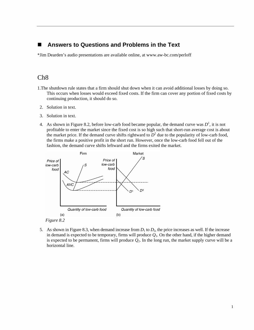
4. As shown in Figure 8.2, before low-carb food became popular, the demand curve was D1, it is not profitable to enter the market since the fixed cost is so high such that short-run average cost is about the market price. If the demand curve shifts rightward to D2 due to the popularity of low-carb food, the firms make a positive profit in the short run. However, once the low-carb food fell out of the fashion, the demand curve shifts leftward and the firms exited the market.

Figure 8.2

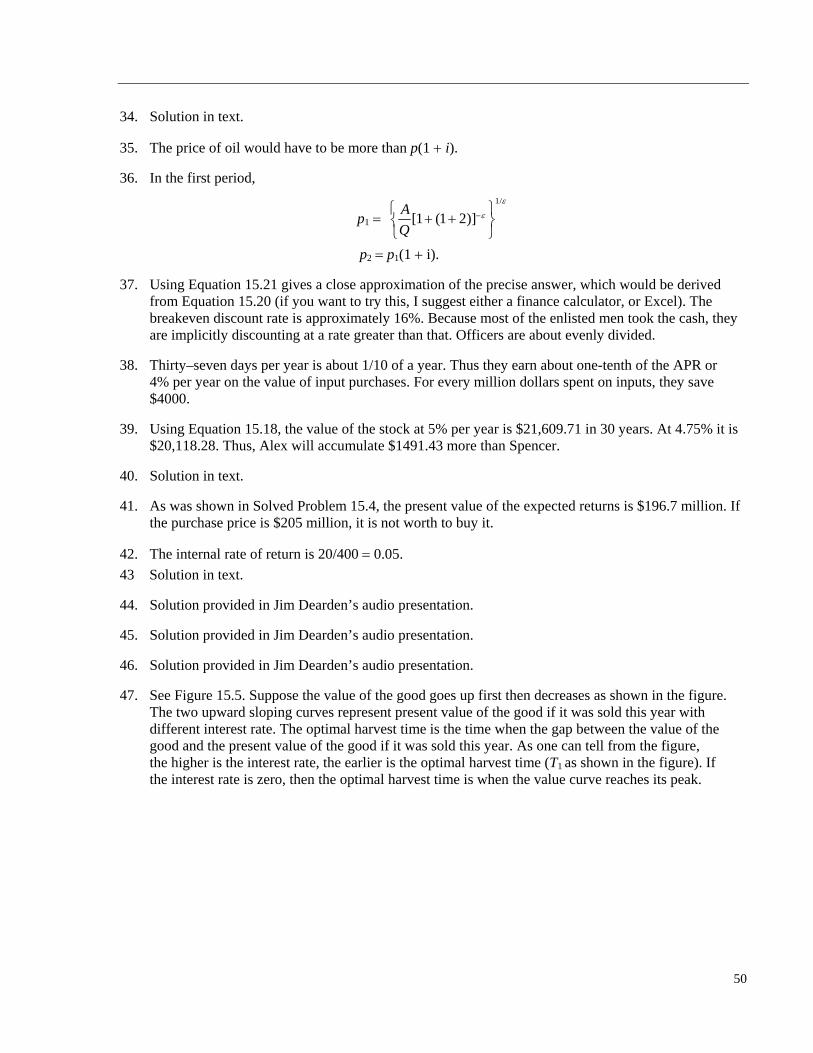
5. As shown in Figure 8.3, when demand increase from D1 to D2, the price increases as well. If the increase in demand is expected to be temporary, firms will produce Q1. On the other hand, if the higher demand is expected to be permanent, firms will produce Q2. In the long run, the market supply curve will be a horizontal line.

1

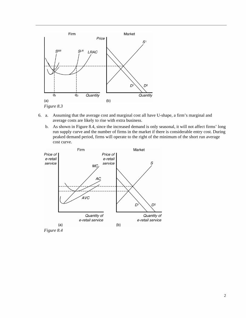
Figure 8.3

6. a. Assuming that the average cost and marginal cost all have U-shape, a firm’s marginal and average costs are likely to rise with extra business.

b. As shown in Figure 8.4, since the increased demand is only seasonal, it will not affect firms’ long run supply curve and the number of firms in the market if there is considerable entry cost. During peaked demand period, firms will operate to the right of the minimum of the short run average cost curve.

Figure 8.4

2

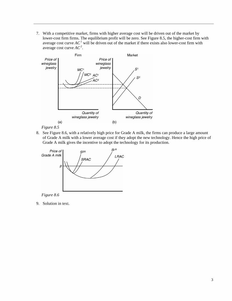
7. With a competitive market, firms with higher average cost will be driven out of the market by lower-cost firm firms. The equilibrium profit will be zero. See Figure 8.5, the higher-cost firm with average cost curve AC 1 will be driven out of the market if there exists also lower-cost firm with average cost curve AC 2.

Figure 8.5

8. See Figure 8.6, with a relatively high price for Grade A milk, the firms can produce a large amount of Grade A milk with a lower average cost if they adopt the new technology. Hence the high price of Grade A milk gives the incentive to adopt the technology for its production.

Figure 8.6


3

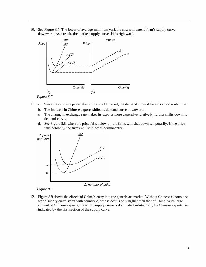
10. See Figure 8.7. The lower of average minimum variable cost will extend firm’s supply curve downward. As a result, the market supply curve shifts rightward.

Figure 8.7

11. a. Since Lesotho is a price taker in the world market, the demand curve it faces is a horizontal line.

b. The increase in Chinese exports shifts its demand curve downward. c. The change in exchange rate makes its exports more expensive relatively, further shifts down its

demand curve. d. See Figure 8.8, when the price falls below p1, the firms will shut down temporarily. If the price

falls below p2, the firms will shut down permanently.

Figure 8.8

12. Figure 8.9 shows the effects of China’s entry into the generic art market. Without Chinese exports, the world supply curve starts with country A, whose cost is only higher than that of China. With large amount of Chinese exports, the world supply curve is dominated substantially by Chinese exports, as indicated by the first section of the supply curve.

4

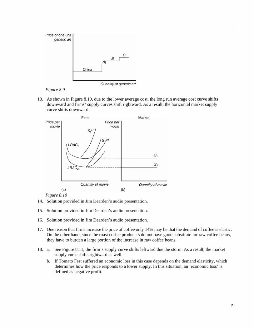
Figure 8.9

13. As shown in Figure 8.10, due to the lower average cost, the long run average cost curve shifts downward and firms’ supply curves shift rightward. As a result, the horizontal market supply curve shifts downward.

Figure 8.10

14. Solution provided in Jim Dearden’s audio presentation.



17. One reason that firms increase the price of coffee only 14% may be that the demand of coffee is elastic. On the other hand, since the roast coffee producers do not have good substitute for raw coffee beans, they have to burden a large portion of the increase in raw coffee beans.

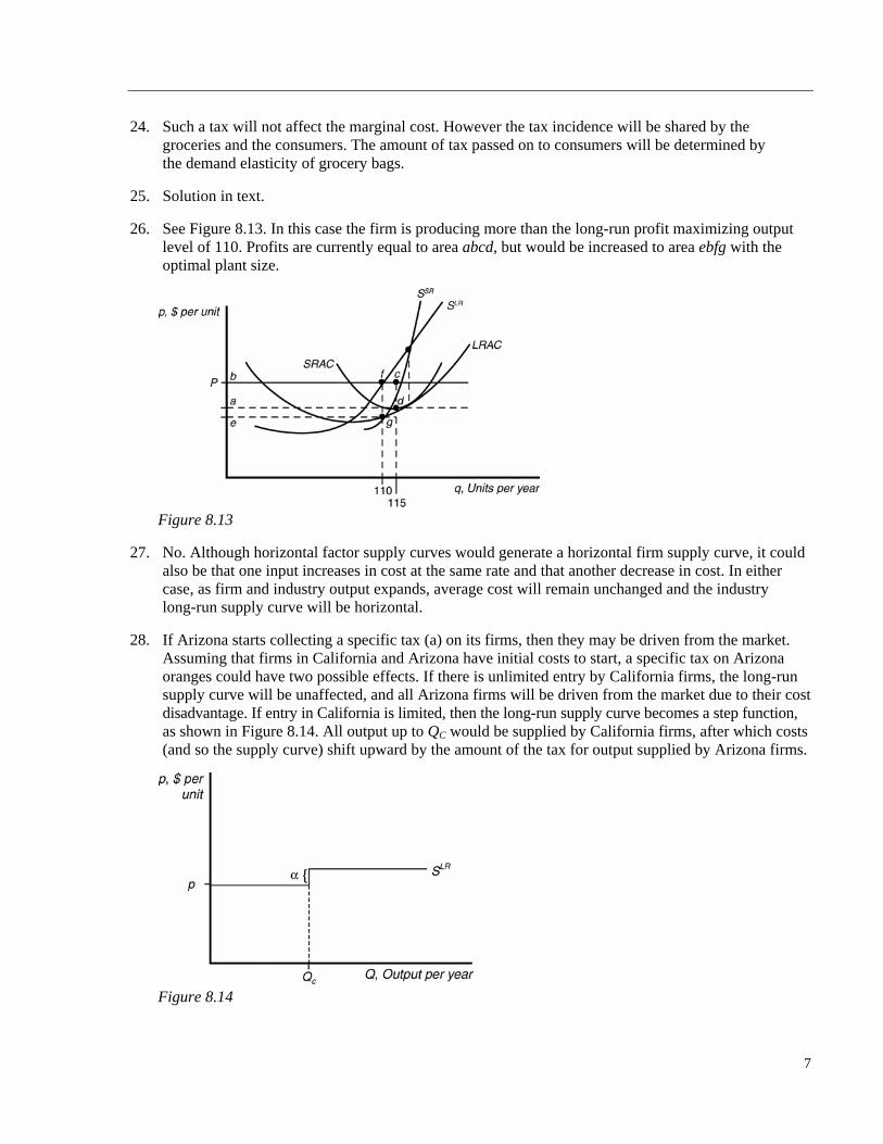
18. a. See Figure 8.11, the firm’s supply curve shifts leftward due the storm. As a result, the market supply curse shifts rightward as well.

b. If Tomato Fest suffered an economic loss in this case depends on the demand elasticity, which determines how the price responds to a lower supply. In this situation, an ‘economic loss’ is defined as negative profit.

5

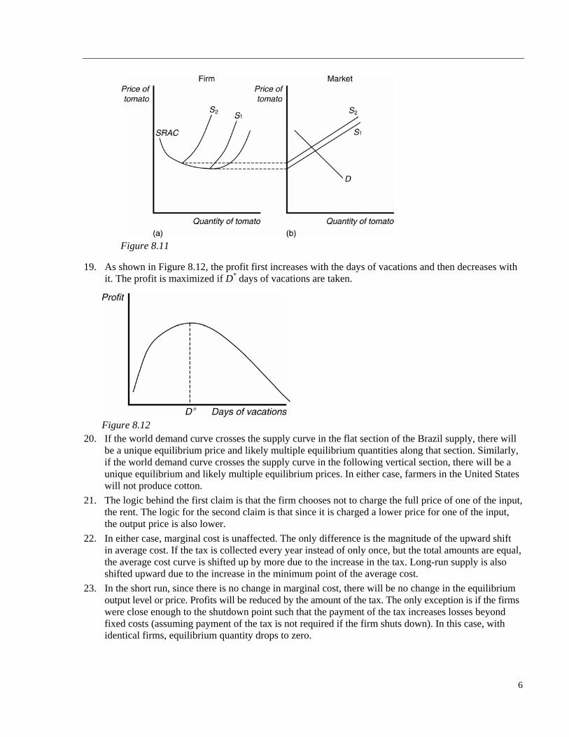
Figure 8.11

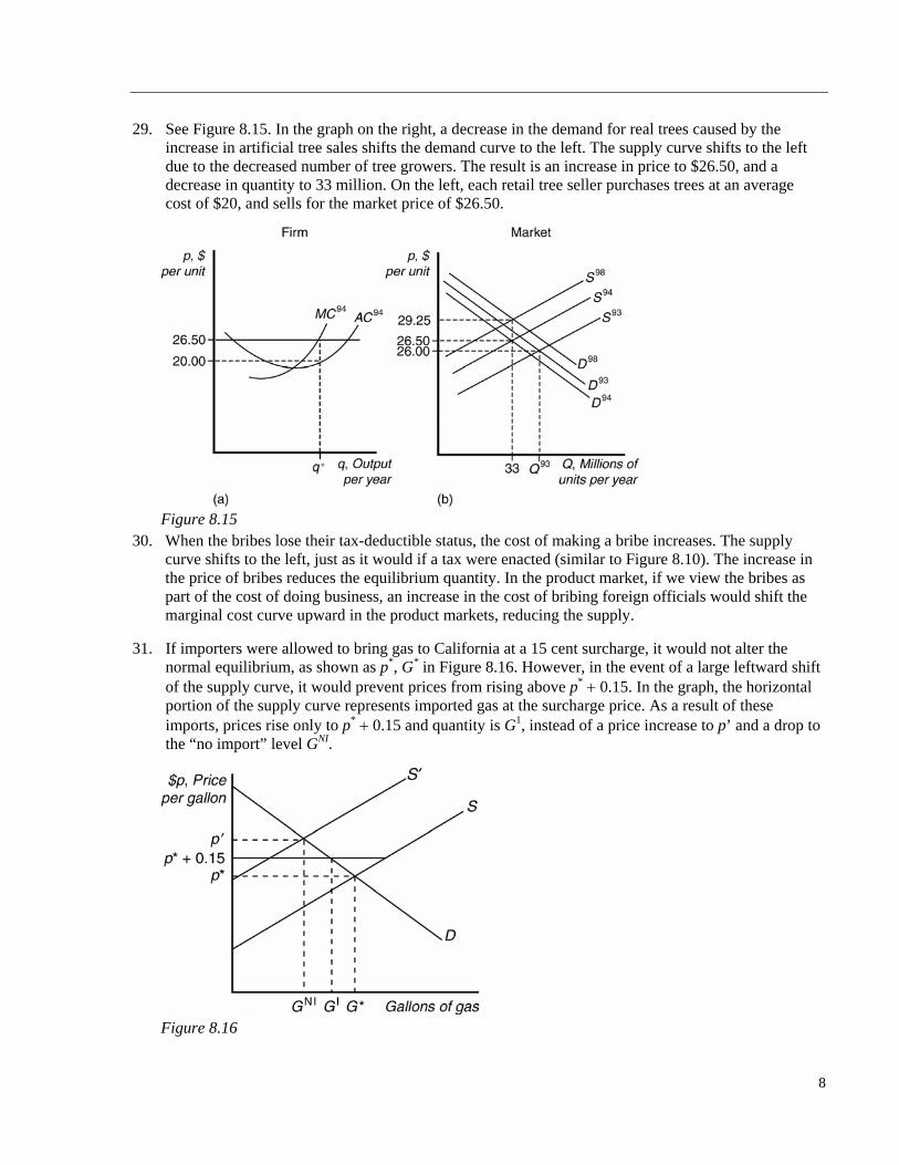
19. As shown in Figure 8.12, the profit first increases with the days of vacations and then decreases with it. The profit is maximized if D* days of vacations are taken.

Figure 8.12

20. If the world demand curve crosses the supply curve in the flat section of the Brazil supply, there will be a unique equilibrium price and likely multiple equilibrium quantities along that section. Similarly, if the world demand curve crosses the supply curve in the following vertical section, there will be a unique equilibrium and likely multiple equilibrium prices. In either case, farmers in the United States will not produce cotton.

21. The logic behind the first claim is that the firm chooses not to charge the full price of one of the input, the rent. The logic for the second claim is that since it is charged a lower price for one of the input, the output price is also lower.

22. In either case, marginal cost is unaffected. The only difference is the magnitude of the upward shift in average cost. If the tax is collected every year instead of only once, but the total amounts are equal, the average cost curve is shifted up by more due to the increase in the tax. Long-run supply is also shifted upward due to the increase in the minimum point of the average cost.

23. In the short run, since there is no change in marginal cost, there will be no change in the equilibrium output level or price. Profits will be reduced by the amount of the tax. The only exception is if the firms were close enough to the shutdown point such that the payment of the tax increases losses beyond fixed costs (assuming payment of the tax is not required if the firm shuts down). In this case, with identical firms, equilibrium quantity drops to zero.

6

24. Such a tax will not affect the marginal cost. However the tax incidence will be shared by the groceries and the consumers. The amount of tax passed on to consumers will be determined by the demand elasticity of grocery bags.


26. See Figure 8.13. In this case the firm is producing more than the long-run profit maximizing output level of 110. Profits are currently equal to area abcd, but would be increased to area ebfg with the optimal plant size.

Figure 8.13

27. No. Although horizontal factor supply curves would generate a horizontal firm supply curve, it could also be that one input increases in cost at the same rate and that another decrease in cost. In either case, as firm and industry output expands, average cost will remain unchanged and the industry long-run supply curve will be horizontal.

28. If Arizona starts collecting a specific tax (a) on its firms, then they may be driven from the market. Assuming that firms in California and Arizona have initial costs to start, a specific tax on Arizona oranges could have two possible effects. If there is unlimited entry by California firms, the long-run supply curve will be unaffected, and all Arizona firms will be driven from the market due to their cost disadvantage. If entry in California is limited, then the long-run supply curve becomes a step function, as shown in Figure 8.14. All output up to QC would be supplied by California firms, after which costs (and so the supply curve) shift upward by the amount of the tax for output supplied by Arizona firms.

Figure 8.14

7

29. See Figure 8.15. In the graph on the right, a decrease in the demand for real trees caused by the increase in artificial tree sales shifts the demand curve to the left. The supply curve shifts to the left due to the decreased number of tree growers. The result is an increase in price to $26.50, and a decrease in quantity to 33 million. On the left, each retail tree seller purchases trees at an average cost of $20, and sells for the market price of $26.50.

Figure 8.15

30. When the bribes lose their tax-deductible status, the cost of making a bribe increases. The supply curve shifts to the left, just as it would if a tax were enacted (similar to Figure 8.10). The increase in the price of bribes reduces the equilibrium quantity. In the product market, if we view the bribes as part of the cost of doing business, an increase in the cost of bribing foreign officials would shift the marginal cost curve upward in the product markets, reducing the supply.

31. If importers were allowed to bring gas to California at a 15 cent surcharge, it would not alter the normal equilibrium, as shown as p*, G* in Figure 8.16. However, in the event of a large leftward shift of the supply curve, it would prevent prices from rising above p* 0.15. In the graph, the horizontal portion of the supply curve represents imported gas at the surcharge price. As a result of these imports, prices rise only to p* 0.15 and quantity is G1, instead of a price increase to p’ and a drop to the “no import” level GNI.

Figure 8.16

8

32. Marginal cost is computed by taking the derivative dC/dq. Profits are maximized by setting MC MR p. For the function given, MC 10 2q q2. Thus profits are maximized when p 10 2q q2. The supply curve is p 10 2q q2 for P 9.25.


34. In the long run price equals marginal cost, and profits are zero. Thus given that industry output Q nq, the following will be true in long-run equilibrium, p 24 nq. Therefore,

24 nq 2q

(24 nq)q 16 q2.

Solving these equations for q, n, Q, and p yields

q 4

n 4

Q 16

p 8. 35. Solution in text.




39. After tax profit is (1 ) ( )pq C q and the profit maximizing output after the tax is imposed is:

( ) ( )(1 ) 0

q Cp

q q

q 1( )(1 ) 0p MC q or

the first order condition. Differentiating this with respect to the ad valorem tax rate yields:

1 2(1 ) ( )(1 ) 0MC q

MC qq

and rearranging:

( )0

(1 )

q MC qMC

q



Ch9

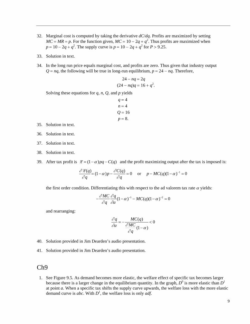
1. See Figure 9.5. As demand becomes more elastic, the welfare effect of specific tax becomes larger because there is a larger change in the equilibrium quantity. In the graph, D0 is more elastic than D1 at point a. When a specific tax shifts the supply curve upwards, the welfare loss with the more elastic demand curve is abc. With D1, the welfare loss is only adf.

9

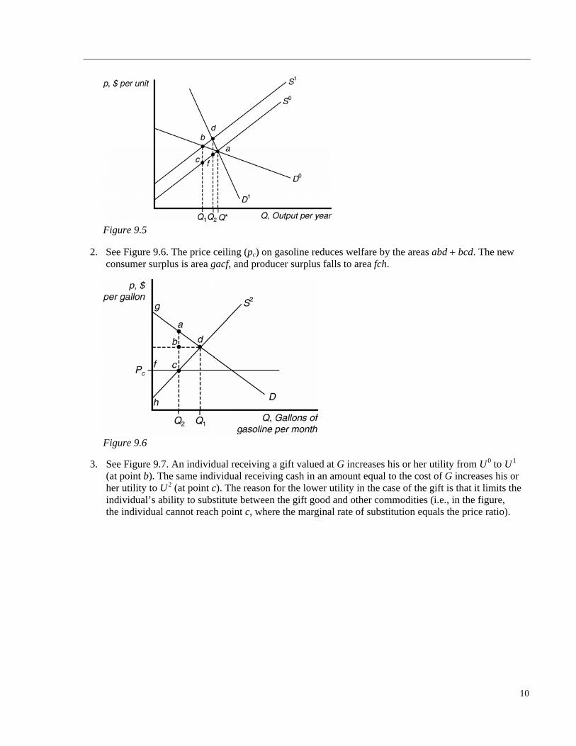
Figure 9.5

2. See Figure 9.6. The price ceiling (pc) on gasoline reduces welfare by the areas abd bcd. The new consumer surplus is area gacf, and producer surplus falls to area fch.

Figure 9.6

3. See Figure 9.7. An individual receiving a gift valued at G increases his or her utility from U0 to U1 (at point b). The same individual receiving cash in an amount equal to the cost of G increases his or her utility to U2 (at point c). The reason for the lower utility in the case of the gift is that it limits the individual’s ability to substitute between the gift good and other commodities (i.e., in the figure, the individual cannot reach point c, where the marginal rate of substitution equals the price ratio).

10

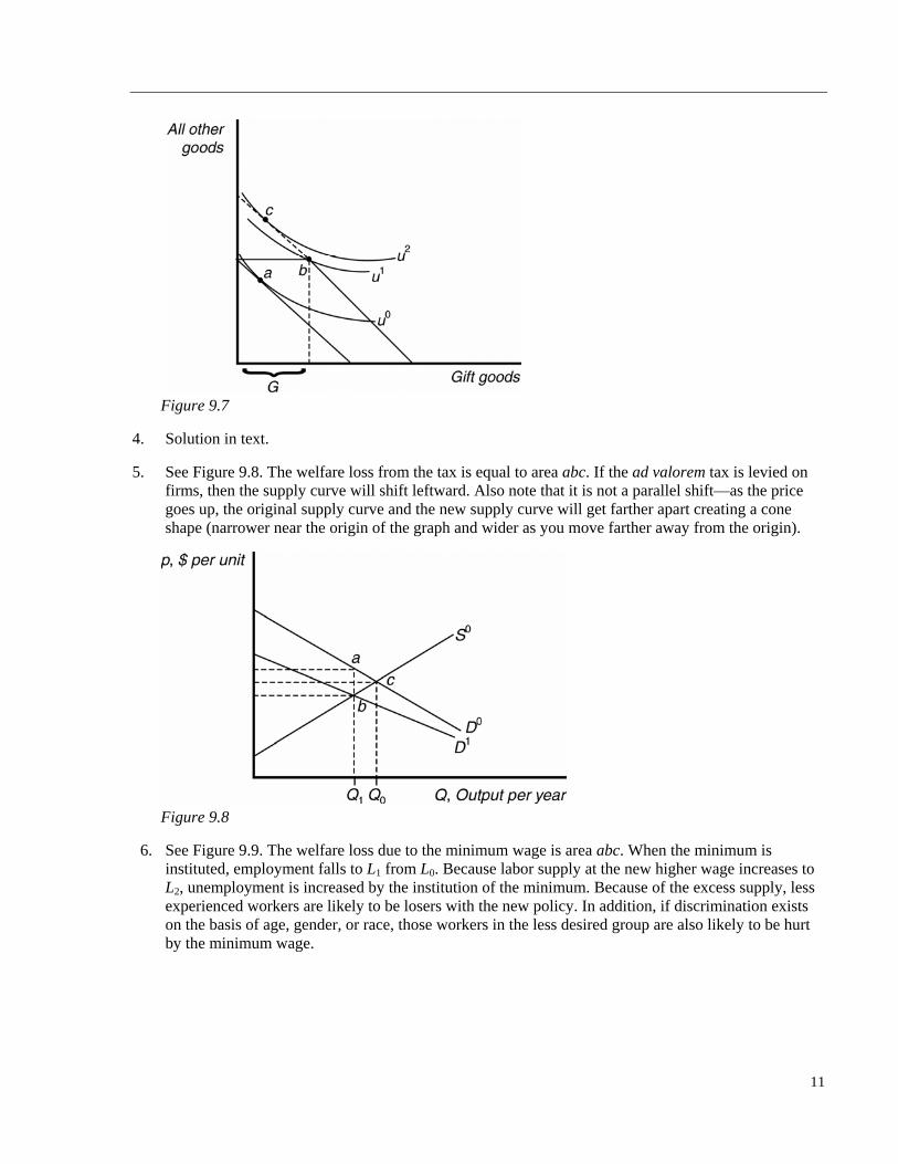
Figure 9.7


5. See Figure 9.8. The welfare loss from the tax is equal to area abc. If the ad valorem tax is levied on firms, then the supply curve will shift leftward. Also note that it is not a parallel shift—as the price goes up, the original supply curve and the new supply curve will get farther apart creating a cone shape (narrower near the origin of the graph and wider as you move farther away from the origin).

Figure 9.8

6. See Figure 9.9. The welfare loss due to the minimum wage is area abc. When the minimum is instituted, employment falls to L1 from L0. Because labor supply at the new higher wage increases to L2, unemployment is increased by the institution of the minimum. Because of the excess supply, less experienced workers are likely to be losers with the new policy. In addition, if discrimination exists on the basis of age, gender, or race, those workers in the less desired group are also likely to be hurt by the minimum wage.

11

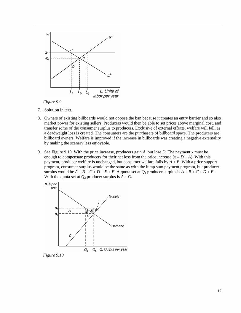
Figure 9.9


8. Owners of existing billboards would not oppose the ban because it creates an entry barrier and so also market power for existing sellers. Producers would then be able to set prices above marginal cost, and transfer some of the consumer surplus to producers. Exclusive of external effects, welfare will fall, as a deadweight loss is created. The consumers are the purchasers of billboard space. The producers are billboard owners. Welfare is improved if the increase in billboards was creating a negative externality by making the scenery less enjoyable.

9. See Figure 9.10. With the price increase, producers gain A, but lose D. The payment x must be enough to compensate producers for their net loss from the price increase (x D A). With this payment, producer welfare is unchanged, but consumer welfare falls by A B. With a price support program, consumer surplus would be the same as with the lump sum payment program, but producer surplus would be A B C D E F. A quota set at Q1 producer surplus is A B C D E. With the quota set at Q2 producer surplus is A C.

Figure 9.10

12

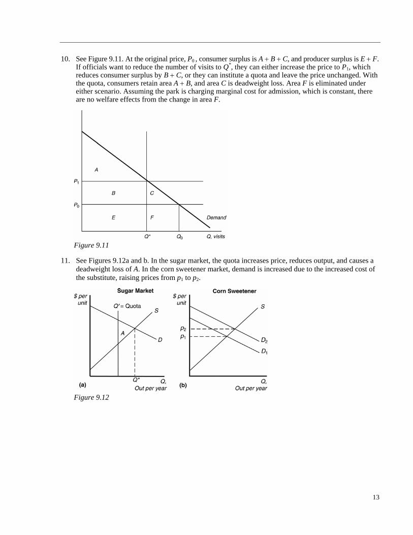
10. See Figure 9.11. At the original price, P0 , consumer surplus is A B C, and producer surplus is E F. If officials want to reduce the number of visits to Q*, they can either increase the price to P1, which reduces consumer surplus by B C, or they can institute a quota and leave the price unchanged. With the quota, consumers retain area A B, and area C is deadweight loss. Area F is eliminated under either scenario. Assuming the park is charging marginal cost for admission, which is constant, there are no welfare effects from the change in area F.

Figure 9.11

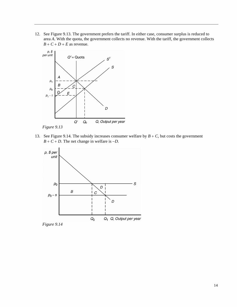
11. See Figures 9.12a and b. In the sugar market, the quota increases price, reduces output, and causes a deadweight loss of A. In the corn sweetener market, demand is increased due to the increased cost of the substitute, raising prices from p1 to p2.

Figure 9.12

13

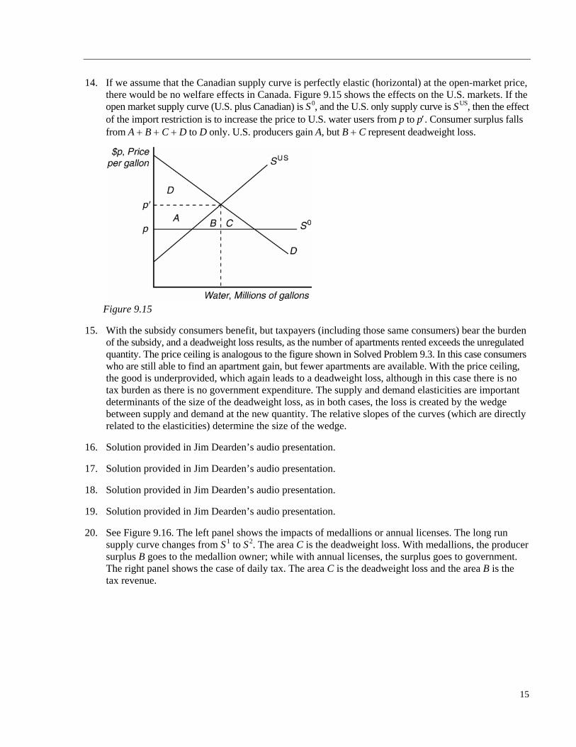
12. See Figure 9.13. The government prefers the tariff. In either case, consumer surplus is reduced to area A. With the quota, the government collects no revenue. With the tariff, the government collects B C D E as revenue.

Figure 9.13

13. See Figure 9.14. The subsidy increases consumer welfare by B C, but costs the government B C D. The net change in welfare is D.

Figure 9.14

14

14. If we assume that the Canadian supply curve is perfectly elastic (horizontal) at the open-market price, there would be no welfare effects in Canada. Figure 9.15 shows the effects on the U.S. markets. If the open market supply curve (U.S. plus Canadian) is S0, and the U.S. only supply curve is SUS, then the effect of the import restriction is to increase the price to U.S. water users from p to p. Consumer surplus falls from A B C D to D only. U.S. producers gain A, but B C represent deadweight loss.

Figure 9.15

15. With the subsidy consumers benefit, but taxpayers (including those same consumers) bear the burden of the subsidy, and a deadweight loss results, as the number of apartments rented exceeds the unregulated quantity. The price ceiling is analogous to the figure shown in Solved Problem 9.3. In this case consumers who are still able to find an apartment gain, but fewer apartments are available. With the price ceiling, the good is underprovided, which again leads to a deadweight loss, although in this case there is no tax burden as there is no government expenditure. The supply and demand elasticities are important determinants of the size of the deadweight loss, as in both cases, the loss is created by the wedge between supply and demand at the new quantity. The relative slopes of the curves (which are directly related to the elasticities) determine the size of the wedge.





20. See Figure 9.16. The left panel shows the impacts of medallions or annual licenses. The long run supply curve changes from S1 to S2. The area C is the deadweight loss. With medallions, the producer surplus B goes to the medallion owner; while with annual licenses, the surplus goes to government. The right panel shows the case of daily tax. The area C is the deadweight loss and the area B is the tax revenue.

15

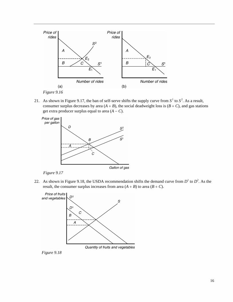
Figure 9.16

21. As shown in Figure 9.17, the ban of self-serve shifts the supply curve from S1 to S2. As a result, consumer surplus decreases by area (A B), the social deadweight loss is (B C), and gas stations get extra producer surplus equal to area (A C).

Figure 9.17

22. As shown in Figure 9.18, the USDA recommendation shifts the demand curve from D1 to D2. As the result, the consumer surplus increases from area (A B) to area (B C).

Figure 9.18

16

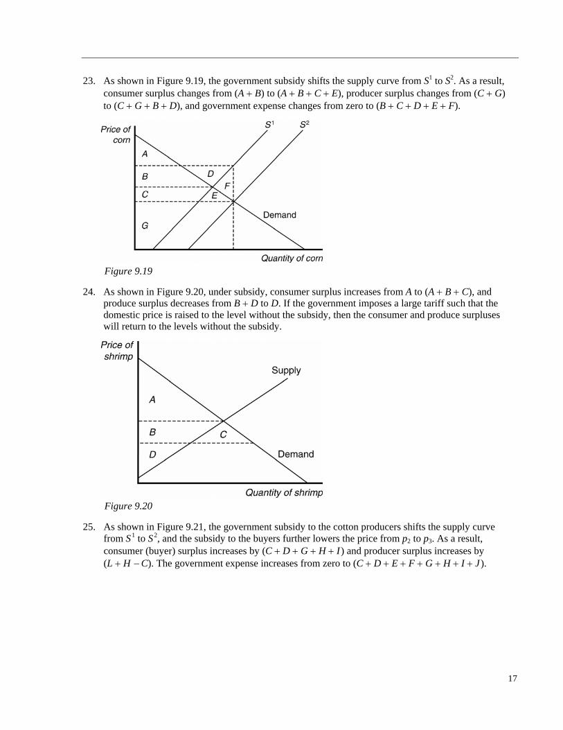
23. As shown in Figure 9.19, the government subsidy shifts the supply curve from S1 to S2. As a result, consumer surplus changes from (A B) to (A B C E), producer surplus changes from (C G) to (C G B D), and government expense changes from zero to (B C D E F).

Figure 9.19

24. As shown in Figure 9.20, under subsidy, consumer surplus increases from A to (A B C), and produce surplus decreases from B D to D. If the government imposes a large tariff such that the domestic price is raised to the level without the subsidy, then the consumer and produce surpluses will return to the levels without the subsidy.

Figure 9.20

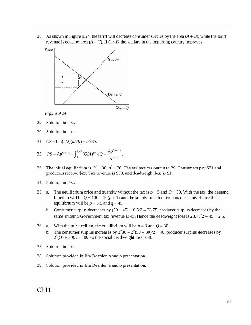
25. As shown in Figure 9.21, the government subsidy to the cotton producers shifts the supply curve from S 1 to S2, and the subsidy to the buyers further lowers the price from p2 to p3. As a result, consumer (buyer) surplus increases by (C D G H I) and producer surplus increases by (L H C). The government expense increases from zero to (C D E F G H I J).

17

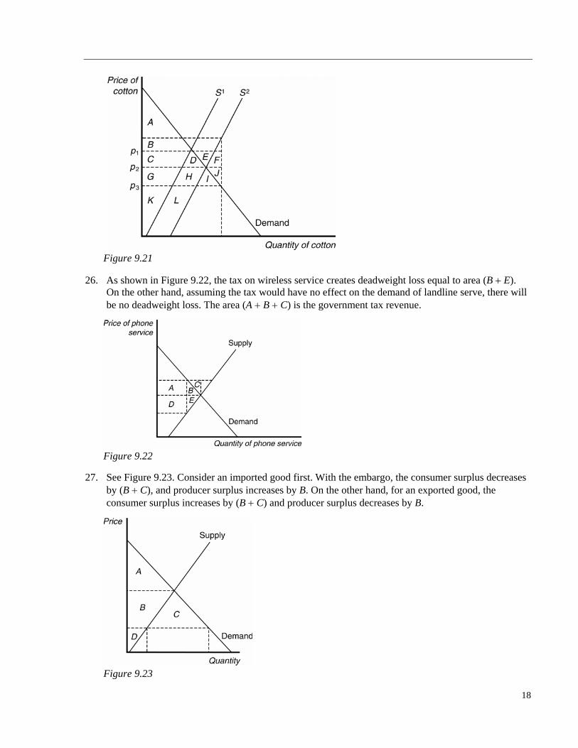
Figure 9.21

26. As shown in Figure 9.22, the tax on wireless service creates deadweight loss equal to area (B E). On the other hand, assuming the tax would have no effect on the demand of landline serve, there will be no deadweight loss. The area (A B C) is the government tax revenue.

Figure 9.22

27. See Figure 9.23. Consider an imported good first. With the embargo, the consumer surplus decreases by (B C), and producer surplus increases by B. On the other hand, for an exported good, the consumer surplus increases by (B C) and producer surplus decreases by B.

Figure 9.23

18

28. As shown in Figure 9.24, the tariff will decrease consumer surplus by the area (A B), while the tariff revenue is equal to area (A C). If C B, the welfare in the importing country improves.

Figure 9.24



31. CS 0.5(a/2)(a/2b) a2/8b.

32. * *( 1)

*( 1) 1/

0( / ) .

1

Ap ApPS Ap Q A dQ

33. The initial equilibrium is Q* 30, p* 30. The tax reduces output to 29. Consumers pay $31 and producers receive $29. Tax revenue is $58, and deadweight loss is $1.


35. a. The equilibrium price and quantity without the tax is p 5 and Q 50. With the tax, the demand function will be Q 100 10(p 1) and the supply function remains the same. Hence the equilibrium will be p 5.5 and q 45.

b. Consumer surplus decreases by (50 45) * 0.5/2 23.75, producer surplus decreases by the

same amount. Government tax revenue is 45. Hence the deadweight loss is 23.75*2 45 2.5.

36. a. With the price ceiling, the equilibrium will be p 3 and Q 30.

b. The consumer surplus increases by 2*30 2*(50 30)/2 40, producer surplus decreases by 2*(50 30)/2 80. So the social deadweight loss is 40.




Ch11

19

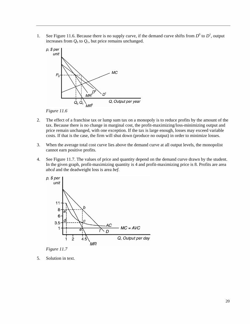
1. See Figure 11.6. Because there is no supply curve, if the demand curve shifts from D0 to D1, output increases from Q0 to Q1, but price remains unchanged.

Figure 11.6

2. The effect of a franchise tax or lump sum tax on a monopoly is to reduce profits by the amount of the tax. Because there is no change in marginal cost, the profit-maximizing/loss-minimizing output and price remain unchanged, with one exception. If the tax is large enough, losses may exceed variable costs. If that is the case, the firm will shut down (produce no output) in order to minimize losses.

3. When the average total cost curve lies above the demand curve at all output levels, the monopolist cannot earn positive profits.

4. See Figure 11.7. The values of price and quantity depend on the demand curve drawn by the student. In the given graph, profit-maximizing quantity is 4 and profit-maximizing price is 8. Profits are area abcd and the deadweight loss is area bef.

Figure 11.7


20

6. No. In order for a firm to be a natural monopoly, its production must exhibit economies of scale, that is, firm’s average cost curve must be downward sloping. If the firm operates in the upward sloping region of its average cost curve, it is possible that two or more firms could produce in the same industry more efficiently than one firm.

7. No. The utility is producing at the section of AC that is upward sloping, and therefore is not a natural monopoly.

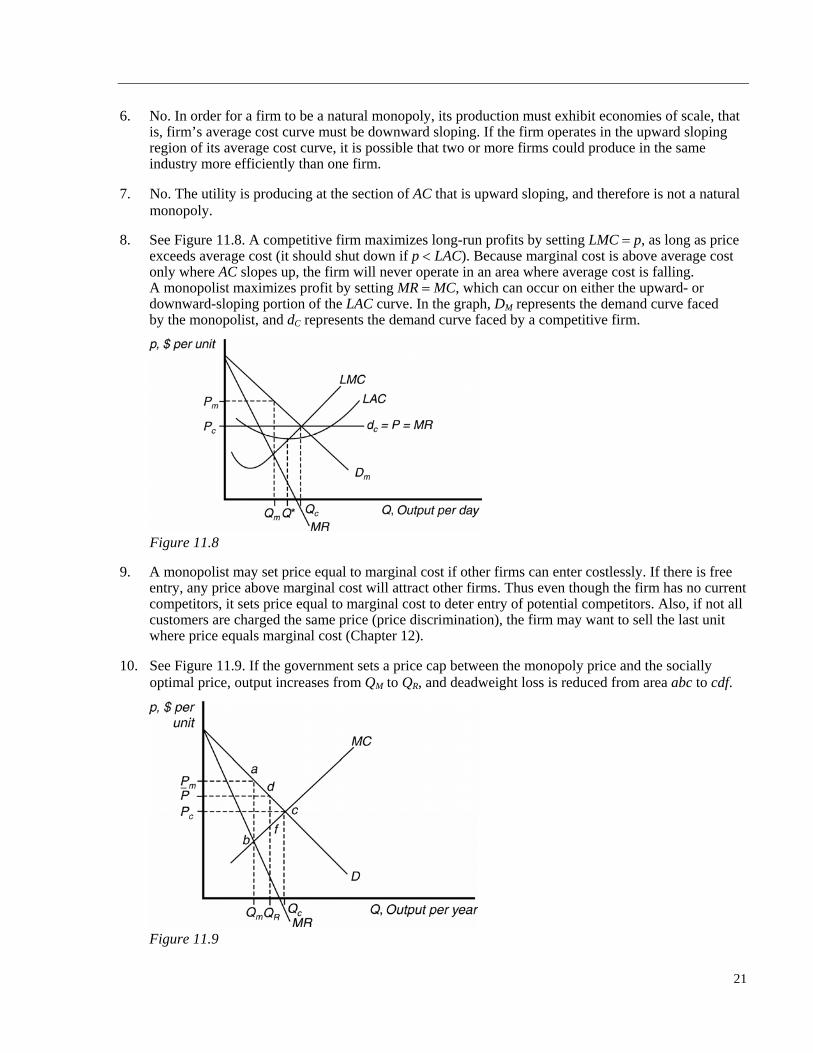
8. See Figure 11.8. A competitive firm maximizes long-run profits by setting LMC p, as long as price exceeds average cost (it should shut down if p LAC). Because marginal cost is above average cost only where AC slopes up, the firm will never operate in an area where average cost is falling. A monopolist maximizes profit by setting MR MC, which can occur on either the upward- or downward-sloping portion of the LAC curve. In the graph, DM represents the demand curve faced by the monopolist, and dC represents the demand curve faced by a competitive firm.

Figure 11.8

9. A monopolist may set price equal to marginal cost if other firms can enter costlessly. If there is free entry, any price above marginal cost will attract other firms. Thus even though the firm has no current competitors, it sets price equal to marginal cost to deter entry of potential competitors. Also, if not all customers are charged the same price (price discrimination), the firm may want to sell the last unit where price equals marginal cost (Chapter 12).

10. See Figure 11.9. If the government sets a price cap between the monopoly price and the socially optimal price, output increases from QM to QR, and deadweight loss is reduced from area abc to cdf.

Figure 11.9

21

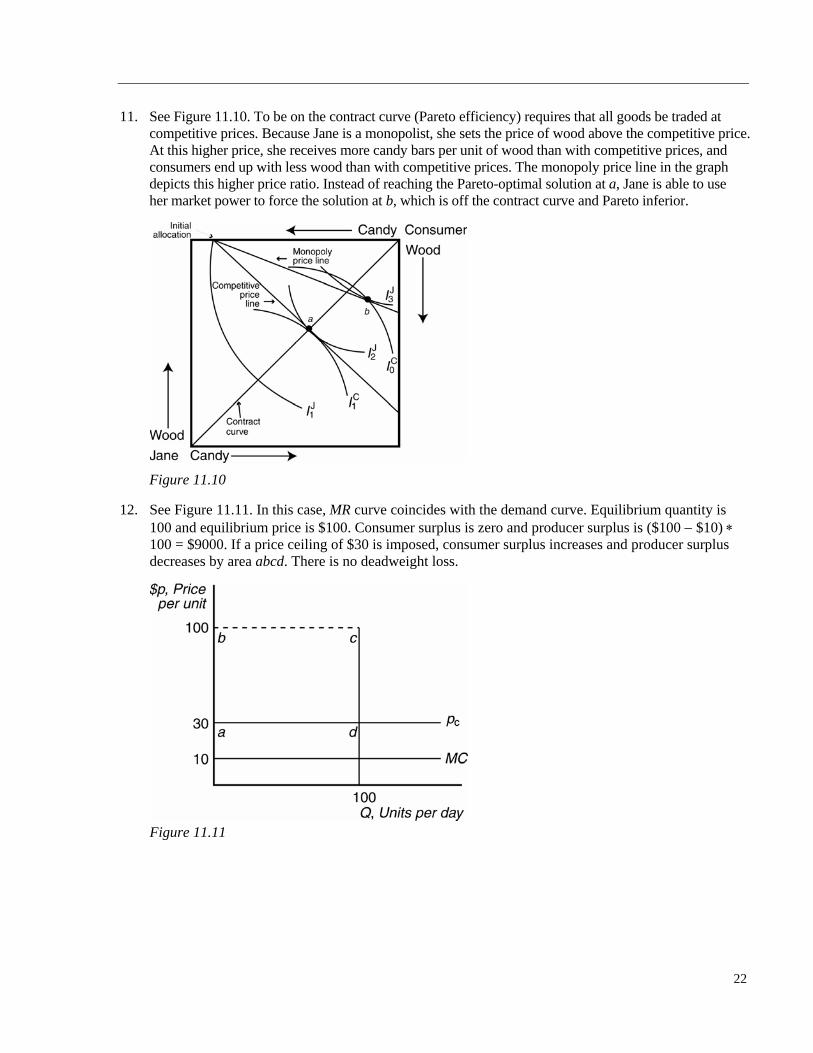
11. See Figure 11.10. To be on the contract curve (Pareto efficiency) requires that all goods be traded at competitive prices. Because Jane is a monopolist, she sets the price of wood above the competitive price. At this higher price, she receives more candy bars per unit of wood than with competitive prices, and consumers end up with less wood than with competitive prices. The monopoly price line in the graph depicts this higher price ratio. Instead of reaching the Pareto-optimal solution at a, Jane is able to use her market power to force the solution at b, which is off the contract curve and Pareto inferior.

Figure 11.10

12. See Figure 11.11. In this case, MR curve coincides with the demand curve. Equilibrium quantity is 100 and equilibrium price is $100. Consumer surplus is zero and producer surplus is ($100 $10) 100 = $9000. If a price ceiling of $30 is imposed, consumer surplus increases and producer surplus decreases by area abcd. There is no deadweight loss.

Figure 11.11

22

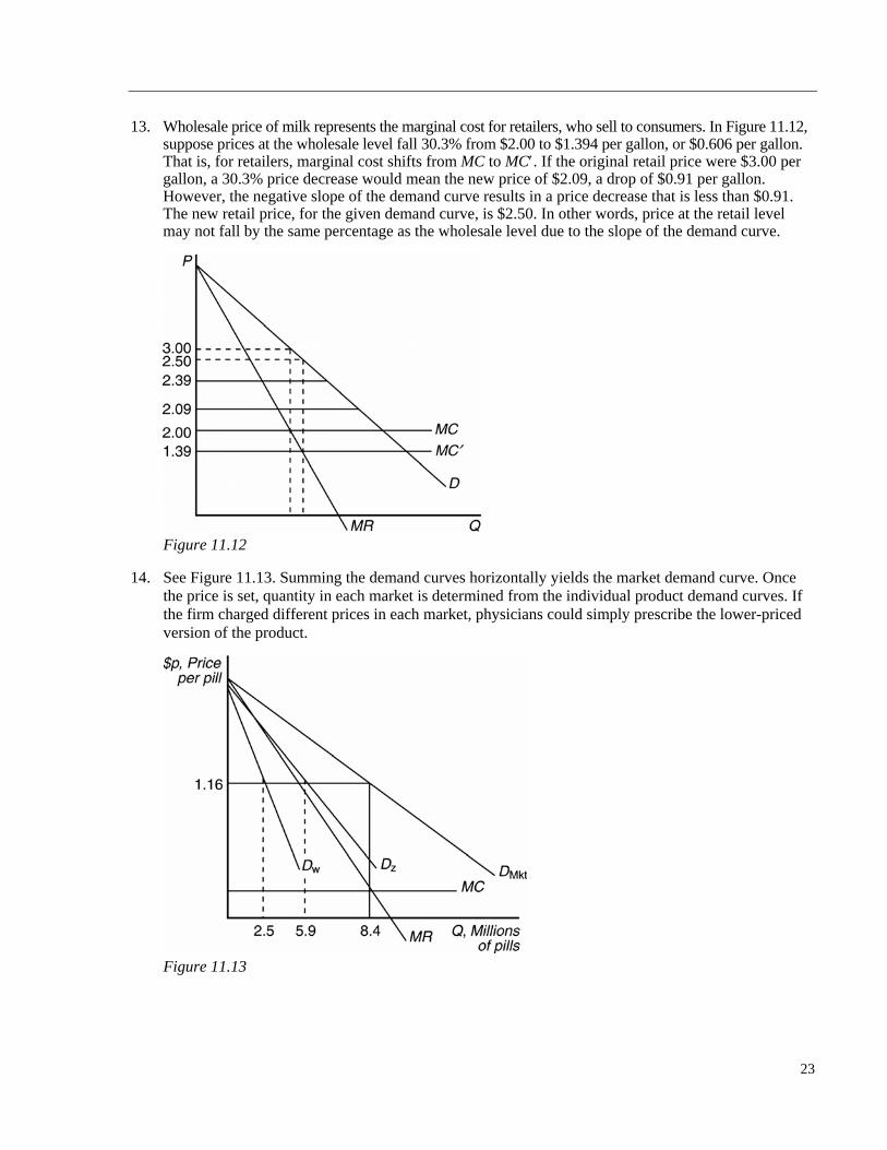
13. Wholesale price of milk represents the marginal cost for retailers, who sell to consumers. In Figure 11.12, suppose prices at the wholesale level fall 30.3% from $2.00 to $1.394 per gallon, or $0.606 per gallon. That is, for retailers, marginal cost shifts from MC to MC. If the original retail price were $3.00 per gallon, a 30.3% price decrease would mean the new price of $2.09, a drop of $0.91 per gallon. However, the negative slope of the demand curve results in a price decrease that is less than $0.91. The new retail price, for the given demand curve, is $2.50. In other words, price at the retail level may not fall by the same percentage as the wholesale level due to the slope of the demand curve.

Figure 11.12

14. See Figure 11.13. Summing the demand curves horizontally yields the market demand curve. Once the price is set, quantity in each market is determined from the individual product demand curves. If the firm charged different prices in each market, physicians could simply prescribe the lower-priced version of the product.

Figure 11.13

23

15. Once a book is online, it is available to consumers for free. As a result, the publisher may loose some consumers after the copyright expires. Limiting the length of a copyright (in the U.S. or elsewhere) would encourage the publisher to charge a higher price for the novel as the publisher attempts to recoup the cost of publishing the novel and earn profit in a shorter period before the copyright expires. After the copyright runs out, the publisher may lower the price of the novel to stay competitive with the online version.

16. This test is relevant because if the club were maximizing revenue, it would be operating at the level MR 0, where the elasticity is 1.

17. Consider a small hotel where the jammer would cost $25,000. If the expected profit from room phone service is $A per day per room and the number of rooms in the hotel is B. Then if $365AB $25,000, it is profitable to install a jammer.

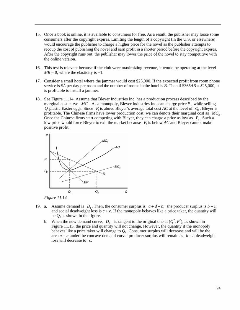
18. See Figure 11.14. Assume that Bleyer Industries Inc. has a production process described by the marginal cost curve 1MC PQ P Q

. As a monopoly, Bleyer Industries Inc. can charge price 1 , while selling 1 plastic Easter eggs. Since 1 is above Bleyer’s average total cost AC at the level of 1 , Bleyer is

profitable. The Chinese firms have lower production cost; we can denote their marginal cost as 2MC

P

. Once the Chinese firms start competing with Bleyer, they can charge a price as low as 2 . Such a low price would force Bleyer to exit the market because is below AC and Bleyer cannot make positive profit.

P2

Figure 11.14

19. a. Assume demand is 1 . Then, the consumer surplus is D ;a d h the producer surplus is b i; and social deadweight loss is c e. If the monopoly behaves like a price taker, the quantity will be Qc as shown in the figure.

b. When the new demand curve, 2 is tangent to the original one at (Q*, P*), as shown in Figure 11.15, the price and quantity will not change. However, the quantity if the monopoly behaves like a price taker will change to Q2. Consumer surplus will decrease and will be the area a h under the concave demand curve; producer surplus will remain as i; deadweight loss will decrease to

,D

b.c

24

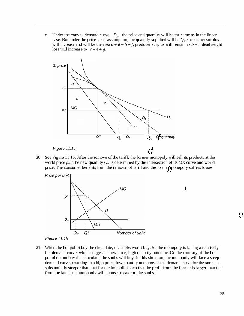
c. Under the convex demand curve, 3 ,D the price and quantity will be the same as in the linear case. But under the price-taker assumption, the quantity supplied will be Q3. Consumer surplus will increase and will be the area a d h f; producer surplus will remain as b i; deadweight loss will increase to e g. c

2Q 3Q

3D

2D

Figure 11.15

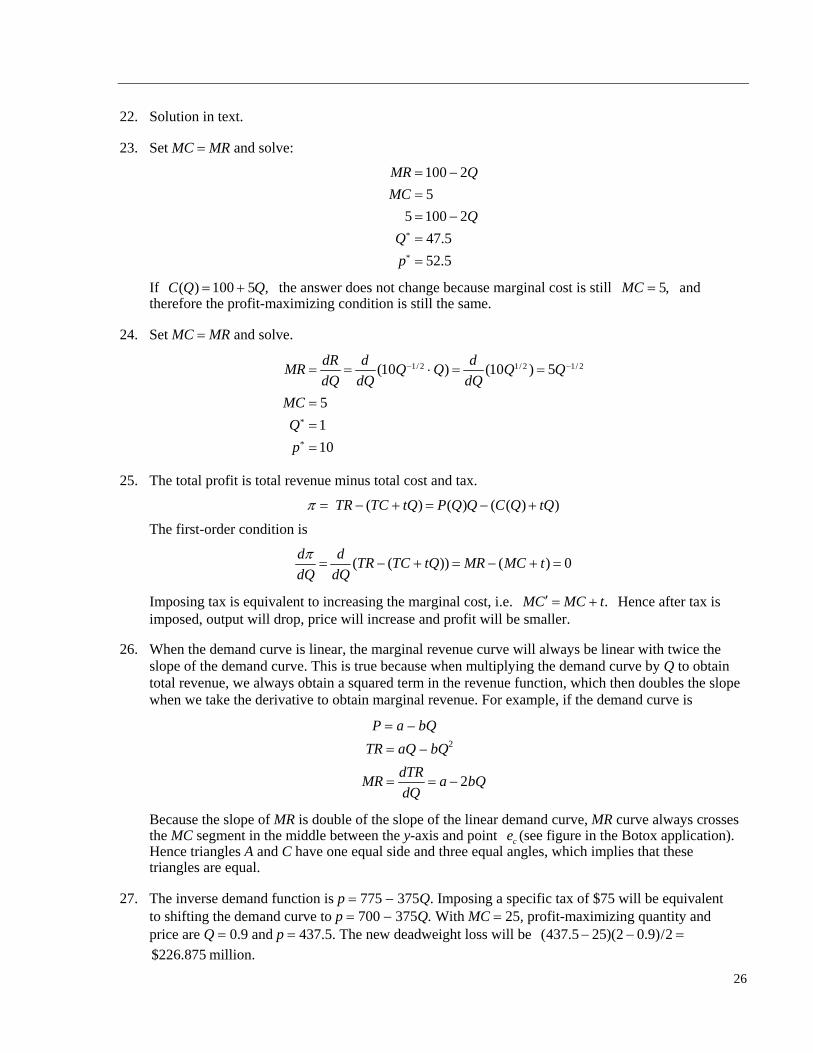
20. See Figure 11.16. After the remove of the tariff, the former monopoly will sell its products at the world price pw. The new quantity Qw is determined by the intersection of its MR curve and world price. The consumer benefits from the removal of tariff and the former monopoly suffers losses.

Figure 11.16

21. When the hoi polloi buy the chocolate, the snobs won’t buy. So the monopoly is facing a relatively flat demand curve, which suggests a low price, high quantity outcome. On the contrary, if the hoi polloi do not buy the chocolate, the snobs will buy. In this situation, the monopoly will face a steep demand curve, resulting in a high price, low quantity outcome. If the demand curve for the snobs is substantially steeper than that for the hoi polloi such that the profit from the former is larger than that from the latter, the monopoly will choose to cater to the snobs.

25


23. Set MC MR and solve:

*

*

100 2

5

5 100 2

47.5

52.5

MR Q

MC

Q

Q

p

If the answer does not change because marginal cost is still and therefore the profit-maximizing condition is still the same.

( ) 100 5 ,C Q Q 5,MC

24. Set MC MR and solve.

1/ 2 1/ 2 1/ 2

*

*

(10 ) (10 ) 5

5

1

10

dR d dMR Q Q Q Q

dQ dQ dQ

MC

Q

p

25. The total profit is total revenue minus total cost and tax.

( ) ( ) ( ( )TR TC tQ P Q Q C Q tQ)

The first-order condition is

( ( )) ( )d d

TR TC tQ MR MC tdQ dQ

0

Imposing tax is equivalent to increasing the marginal cost, i.e. .MC MC t Hence after tax is imposed, output will drop, price will increase and profit will be smaller.

26. When the demand curve is linear, the marginal revenue curve will always be linear with twice the slope of the demand curve. This is true because when multiplying the demand curve by Q to obtain total revenue, we always obtain a squared term in the revenue function, which then doubles the slope when we take the derivative to obtain marginal revenue. For example, if the demand curve is

P a – bQ

TR aQ – bQ2

2dTR

MR adQ

bQ

Because the slope of MR is double of the slope of the linear demand curve, MR curve always crosses the MC segment in the middle between the y-axis and point c (see figure in the Botox application). Hence triangles A and C have one equal side and three equal angles, which implies that these triangles are equal.

e

27. The inverse demand function is p 775 375Q. Imposing a specific tax of $75 will be equivalent to shifting the demand curve to p 700 375Q. With MC 25, profit-maximizing quantity and price are Q 0.9 and p 437.5. The new deadweight loss will be

million.

(437.5 25)(2 0.9)/2 $226.875

26

28. With a price ceiling of $200, monopoly will produce Q (775 200)/375 1.53 million vials and the deadweight loss will be (200 – 25) * (2 1.53)/2 $41.1 million.



31. The price/marginal cost ratio is 99/45.37 2.18. Lerner Index is / 99 45.37/99 0.542.P MC P Using the formula for the Lerner Index, the elasticity is .85.


33. The Lerner Index is (1840.8 100)/1840.8 0.95. Hence Tenet believes that the elasticity it faces is 1.06.

34. The price/marginal cost ratio is 5000/2000 2.5. The Lerner Index is (5000 2000)/5000 0.6. Hence Segway believes it faces a demand elasticity of 1.67.

35. The price/marginal cost ratio is 499/258 1.93. The Lerner Index is (499 258)/499 0.48, and the elasticity Apple believes it faces is 2.08.

36. The Lerner Index is (84.95 37)/84.95 0.56. Hence Stamps.com believes that it faces a demand elasticity of 1.79.


38. In the competitive case, equilibrium is found by equating supply and demand curves, D S:

1.787 0.0004641 0.496 0.00020165Q Q

Then

*

*

3429.2151 lb

0.19550 $/lbC

C

Q

P

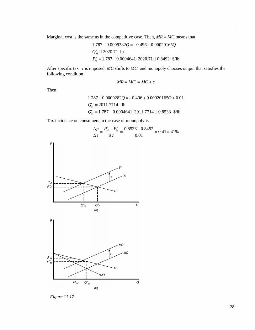
Once the specific tax $0.01 is imposed, the supply curve, which is also MC, shifts up (see Figure 11.17a). To find the after-tax equilibrium, we solve

1.787 0.0004641 0.496 0.00020165 0.01

3414.1945 lb

0.20247 $/lbC

C

D S S

Q Q

Q

P

This suggests that tax incidence in the case of competition is

* 0.20247 0.195500.7 70%

0.01C CP Pp

In the monopoly case, pretax profit-maximizing output and price levels are found by equating MC and MR (see Figure 11.17b). Marginal revenue is

( ( ) ) ((1.787 0.0004641 ) )

1.787 0.0009282

dR d dMR P Q Q Q Q

dQ dQ dQ

Q

27

Marginal cost is the same as in the competitive case. Then, MR MC means that

*

*

1.787 0.0009282 0.496 0.00020165

2020.71 lb

1.787 0.0004641 2020.71 0.8492 $/lbM

M

Q Q

Q

P

After specific tax is imposed, MC shifts to MC and monopoly chooses output that satisfies the following condition

MR MC MC

Then

1.787 0.0009282 0.496 0.00020165 0.01

2011.7714 lb

1.787 0.0004641 2011.7714 0.8533 $/lbM

M

Q Q

Q

Q

Tax incidence on consumers in the case of monopoly is

* 0.8533 0.84920.41 41%

0.01M MP Pp

Figure 11.17

28

39. Consider constant marginal cost and suppose the monopoly is facing a linear demand function with inverse demand function p a bQ. The monopoly will produce Q (MC a)/2b, where MC is the lower of two marginal cost at the factory with lower MC, and zero unit at the factor with higher MC. Suppose both factories have increasing marginal cost, the monopoly will produce at two factories Q1 and Q2 such that MC(Q1) MC(Q2) MC.

40. a. If the consumer cannot steal music, the total demand function function will be p 120 Q/2. The monopoly will set MR 120 Q 20, such that Q 100 and p 70. Consumer surplus will be 2500, profit and producer surplus will be 5000, and deadweight loss will be 2500.

b. If the dishonest customer can steal music, then the total demand function will be p 120 Q. The monopoly will set MR 120 2Q 20, such that Q 50 and p 70.

c. When dishonest customers can pirate the music, consumer surplus will consist of consumer surplus of honest and dishonest customers. Consumer surplus of dishonest customers will be 7200 and consumer surplus of honest customers will be 1250; therefore, total consumer surplus will be 7200 1250 8450. Producer will receive profit and surplus only by selling to the honest customers. Profit and producer surplus will be 2500. Deadweight loss will be 1250.


42. a. To solve for the expansion path, set the ratio of the marginal products equal to the ratio of the input prices (see Appendix 7C)

L

K

MP

MP r

This gives the equation for the expansion path 0.25K Lr

L

. See Figure 11.18.

b. Substituting the expansion path into the production function yields L 2Q, and K 0.5Q. Thus C(Q) wL rK w2Q r 0.5Q 1(2)Q 4(0.5)Q 4Q.

c. Long-run profit-maximizing output is where LMC MR.

2

4

( ( ) ) (100 ) 100 2

dCLMC

dQ

dR d dMR P Q Q Q Q

dQ dQ dQ

Q

Q* 48

p* 52

29

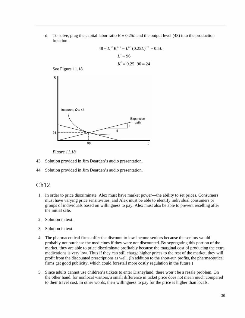
d. To solve, plug the capital labor ratio K 0.25L and the output level (48) into the production function.

1/ 2 1/ 2 1/ 2 1/ 248 (0.25 ) 0.5L K L L L

L* 96

K* 0.25 96 24 See Figure 11.18.

Figure 11.18



Ch12

1. In order to price discriminate, Alex must have market power—the ability to set prices. Consumers must have varying price sensitivities, and Alex must be able to identify individual consumers or groups of individuals based on willingness to pay. Alex must also be able to prevent reselling after the initial sale.



4. The pharmaceutical firms offer the discount to low-income seniors because the seniors would probably not purchase the medicines if they were not discounted. By segregating this portion of the market, they are able to price discriminate profitably because the marginal cost of producing the extra medications is very low. Thus if they can still charge higher prices to the rest of the market, they will profit from the discounted prescriptions as well. (In addition to the short-run profits, the pharmaceutical firms get good publicity, which could forestall more costly regulation in the future.)

5. Since adults cannot use children’s tickets to enter Disneyland, there won’t be a resale problem. On the other hand, for nonlocal visitors, a small difference in ticket price does not mean much compared to their travel cost. In other words, their willingness to pay for the price is higher than locals.

30

6. When there is a big price different across the border and shipping the car from Canada to the United States is relatively cheap, consumers in Canada are able to make a profit by reselling their cars in the United States. To prevent this kind of resale that would decrease Ford’s profit from price discrimination, Ford required Canadian dealer to sign an agreement that prohibited moving vehicles to the United States. Since the prevention might not be effective, in the following year, Ford cut the supply in Canada to only 2000 cars to practically eliminate the resale problem.

7. If Amazon can effectively monitor individual customer’s shopping pattern and history and offer a different price accordingly, this is essentially first-degree price discrimination.

8. If the difference in the cost of a car renting service is equal to the difference in the rental price between the two cities, then there is no price discrimination. Otherwise, there may be price discrimination, especially as resales of the service is practically impossible.

9. Lower profit margin indicates the PC market is becoming more competitive. In other words, the market power of PC producers is decreasing, therefore lowering their ability to price discriminate.

10. a. This is third degree price discrimination. Suppose 1000 tickets were available, then price is determined by the bidder with the 1000th highest willingness-to-pay. All bidders with higher willingness-to-pay get the same price.

b. This is first degree price discrimination as each bidder is charged at a price equal to his or her willingness-to-pay.

11. The difference in profit between a single price monopoly and perfect price discrimination is the area A and C in the application, which is $375 million.

12. The union can set the price at the level w* where demand and supply curves cross and request a lump-sum contribution whose total is equal to the area below the demand curve and above the price level w*. If the workers are not identical, say, if their ages are different, then the value of that uniform lump sum contribution may be different for different workers.

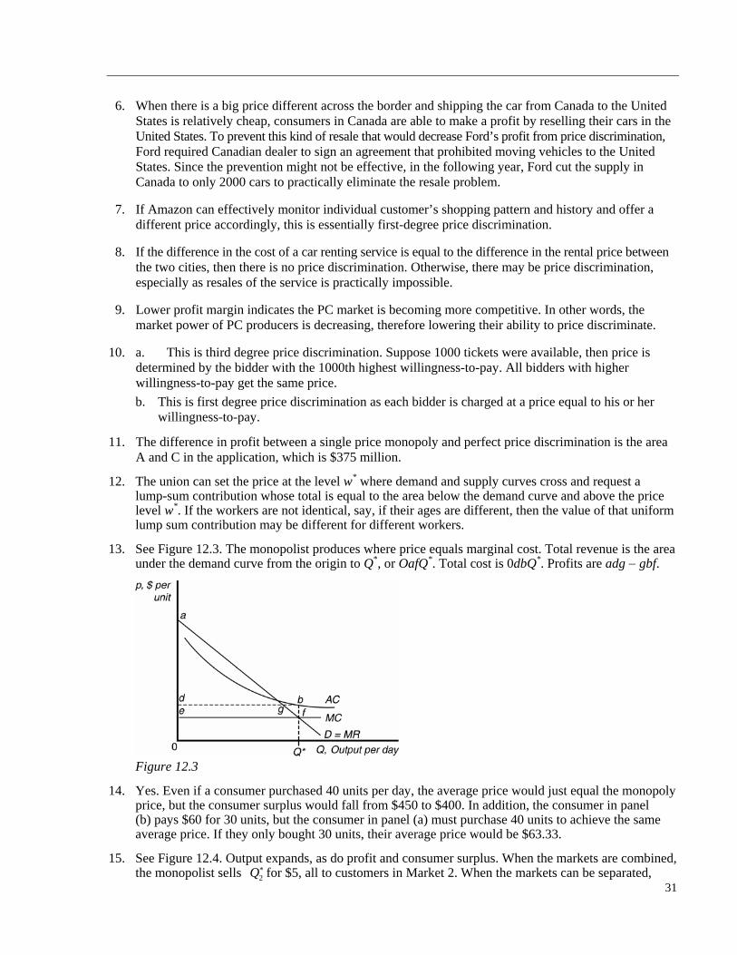
13. See Figure 12.3. The monopolist produces where price equals marginal cost. Total revenue is the area under the demand curve from the origin to Q*, or OafQ*. Total cost is 0dbQ*. Profits are adg gbf.

Figure 12.3

14. Yes. Even if a consumer purchased 40 units per day, the average price would just equal the monopoly price, but the consumer surplus would fall from $450 to $400. In addition, the consumer in panel (b) pays $60 for 30 units, but the consumer in panel (a) must purchase 40 units to achieve the same average price. If they only bought 30 units, their average price would be $63.33.

31

15. See Figure 12.4. Output expands, as do profit and consumer surplus. When the markets are combined, the monopolist sells for $5, all to customers in Market 2. When the markets can be separated, *

2Q

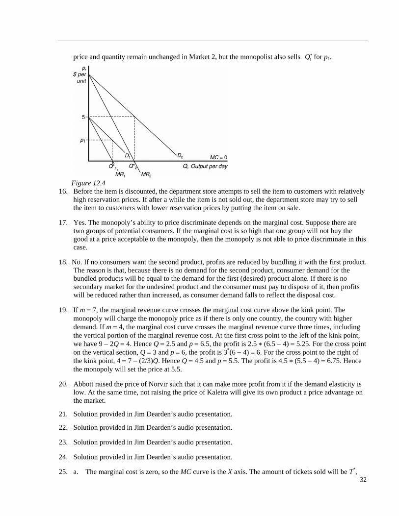
32

*price and quantity remain unchanged in Market 2, but the monopolist also sells for p1. 1Q

Figure 12.4

16. Before the item is discounted, the department store attempts to sell the item to customers with relatively high reservation prices. If after a while the item is not sold out, the department store may try to sell the item to customers with lower reservation prices by putting the item on sale.

17. Yes. The monopoly’s ability to price discriminate depends on the marginal cost. Suppose there are two groups of potential consumers. If the marginal cost is so high that one group will not buy the good at a price acceptable to the monopoly, then the monopoly is not able to price discriminate in this case.

18. No. If no consumers want the second product, profits are reduced by bundling it with the first product. The reason is that, because there is no demand for the second product, consumer demand for the bundled products will be equal to the demand for the first (desired) product alone. If there is no secondary market for the undesired product and the consumer must pay to dispose of it, then profits will be reduced rather than increased, as consumer demand falls to reflect the disposal cost.

19. If m 7, the marginal revenue curve crosses the marginal cost curve above the kink point. The monopoly will charge the monopoly price as if there is only one country, the country with higher demand. If m 4, the marginal cost curve crosses the marginal revenue curve three times, including the vertical portion of the marginal revenue cost. At the first cross point to the left of the kink point, we have 9 2Q 4. Hence Q 2.5 and p 6.5, the profit is 2.5 * (6.5 4) 5.25. For the cross point on the vertical section, Q 3 and p 6, the profit is 3*(6 4) 6. For the cross point to the right of the kink point, 4 7 (2/3)Q. Hence Q 4.5 and p 5.5. The profit is 4.5 * (5.5 4) 6.75. Hence the monopoly will set the price at 5.5.

20. Abbott raised the price of Norvir such that it can make more profit from it if the demand elasticity is low. At the same time, not raising the price of Kaletra will give its own product a price advantage on the market.





25. a. The marginal cost is zero, so the MC curve is the X axis. The amount of tickets sold will be T*,

where the MR curve intersects X axis.

b. The concerts’ failure may indicate monopoly price, but not that the monopoly set too high a price.

c. If the monopoly can perfectly price discriminate, it can obtain all the producer surplus below the demand curve.

26. No, it is not reasonable to conclude that U.S. drivers subsidize European gasoline prices. If oil companies have market power in the United States and Europe and can price discriminate, they will treat each market as a separate market setting prices and quantities at profit-maximizing levels independent of the other market.

27. One possible explanation for higher magazine prices at a newsstand, rather than through a subscription, is the higher transaction cost of selling magazines through a network of newsstands. Besides the transaction cost, the desire to increase magazine sales that influences publisher’s ability to attract advertising revenue is another strong motivator to lower the price of a subscription.




31. The price charged in Canada is $15 * (1 33%) 20. Using Formula (12.2), we can get the elasticity of Canadian consumer is 1.05. The price charged in Japan is $25, hence the elasticity is 25/24 1.04.


33. Setting marginal revenue equal to marginal cost yields Q* 30, p* 60. Profit is $900, consumer surplus is $450, welfare is $1350 (PS CS), and deadweight loss is $450.

34. The profit function of the monopoly described in Figure 12.3 is

1 1 2 2 1 3 3 2 3p Q p Q Q p Q Q mQ

The monopoly faces a demand curve 90p Q . Then, 90Q p and we can write

1 1

2 2

3 3

90

90

90

Q p

Q p

Q p

Using these expressions, the profit function can be rewritten as

1 1 2 2 1 3 3 2

1 1 2 1 2 3 2 3 3

2 2 21 1 1 2 2 2 3 3 3

90 90 90 90 90 90

90 90

90 90

3p p p p p p p p m p

p p p p p p p p m p

p p p p p p p p m mp

FOC:

33

1 21

1 2 32

2 33

90 2 0

2 0

2 0

p pp

p p pp

p p mp

Here Solving simultaneously, we find that profit-maximizing prices are 30.m 1 75,p 2 60,p

and 3 45.p

35. a. The monopoly can set the price to be 60 and the minimum amount to be 60 such that to achieve the same outcome as in perfect price discrimination case.

b. For a initial price of 90, the total demand will be zero. 36. Using Equation 12.2,

pUS (1 – 1/2) 10 pJ (1 – 1/5) pUS $20, pJ $12.50.

37. Set marginal revenue in each market equal to marginal cost to determine the quantities. Plug the quantities into the demand functions to determine prices.

MR1 100 – 2Q1 30 MC

MR2 120 – 4Q2 30 MC

Q1 35; p1 65

Q2 22.5; p2 75

38. Marginal revenue depends on price and elasticity of demand:

11

1

22

2

11

11

MR p

MR p

From Solved Problem 12.3 we know that 1 2 60p p 1

. Since multimarket price discrimination leads to prices that equate marginal revenues, that is, 2MR MR , we may write

1 21 2

1 2

1 2

1 11 1

1 160 1 60 1

p p

39. Suppose a two-part tariff includes a fixed entry fee F, plus a per-unit cost m. In this case, the average price per unit is F/q m, which exceeds the marginal price m. Thus consumers who purchase more units pay a lower average or per-unit price.

34

35

1

40. See figure in Solved Problem 12.4. Without advertising, the optimal number of subscriptions is determined by the intercept of MMR and C . This gives optimal output and price levels and 1Q 1.p Presence of advertising has the same effect on the demand curve as a subsidy, that is, demand shifts outward, from to The new optimal point is set by the intercept of 1D 2 2.D MR and .MC With

advertising, the new equilibrium is a pair and 2Q 2.p Increasing increases subscriptions a

41. Giving a lump-sum subsidy to Canadian publishers lowers their marginal cost regardless of how many subscriptions they sell. If MC drops, the publisher can charge a lower price for a subscription, which will increase subscription sales.

42. Assume one unit of advertising costs $1. Then monopoly solves

,max ( , ) ( )

p AR p A C p A

First order conditions are

0

1 0

R dC

p p dp

R

A A

A pair *p and that solves the first order conditions maximizes monopoly’s profit. *A

43. Assume one unit of advertising costs $1. The profit function is

p (100 – Q A1/2 )Q – 10Q – A

The resulting first-order conditions are

p/A (Q/2)A–1/2 – 1 0

p/Q 100 – 2Q A1/2 – 10 0

A* 900

Q* 60

p* 70

44. Given the demand and cost information, the profit function is

p (a – bQ cAa )Q – mQ – A

The resulting first-order conditions are

p/A acQAa–1 – 1 0 p/Q a – 2bQ cAa – m 0

Solving for A* and Q* yields

A* (acQ*)–(1/a–1)

with Q* is solution to (a – m) – 2bQ c(acQ*)–(a/a–1) 0.

45. If pharmaceutical firms are rational, then they advertise because advertising increases their profit. Profit is revenue less total cost. It is reasonable then to infer that as sales increase due to advertising, production and distribution costs of pharmaceutical companies increase slower than revenue.



Ch13

1.See Figure 13.1 in the text. Each cartel member has incentive to cheat, reasoning that one country increasing the output will not change the price much. At the same time, since the marginal revenue is above marginal cost, by producing more oil than the agreed upon amount, it can make additional profit.


3. One possibility is that at for places with relatively larger number of firms, the market is segmented. In each market segment, the number of firms is smaller and therefore, they are able to collude and charge a higher price.

4. With only one firm, the deadweight loss is equal to the deadweight loss of a monopoly, that is, (243 147) * (192 96)/2 (243 147) * (243 147)/2 4608 (see Figure 13.2 a in the text). With three firms, the deadweight loss is (195 147) * (195 147)/2 1152, decreasing by 75%.

36

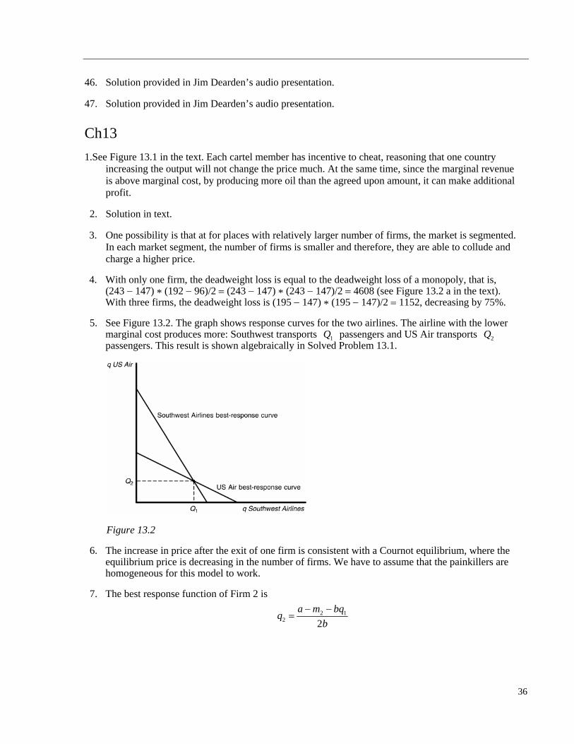
Q Q 5. See Figure 13.2. The graph shows response curves for the two airlines. The airline with the lower

marginal cost produces more: Southwest transports 1 passengers and US Air transports passengers. This result is shown algebraically in Solved Problem 13.1.

2

Figure 13.2

6. The increase in price after the exit of one firm is consistent with a Cournot equilibrium, where the equilibrium price is decreasing in the number of firms. We have to assume that the painkillers are homogeneous for this model to work.

7. The best response function of Firm 2 is

2 12 2

qb

a m bq

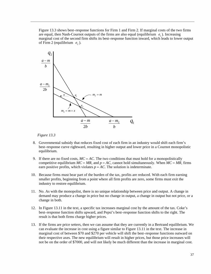
Figure 13.3 shows best–response functions for Firm 1 and Firm 2. If marginal costs of the two firms are equal, then Nash-Cournot outputs of the firms are also equal (equilibrium 1 ). Increasing marginal cost of the second firm shifts its best–response function inward, which leads to lower output of Firm 2 (equilibrium ).

e

2e

a m

b

x1e

2q

1q2

a m

b

2

2

a m

b

2a m

b

2e

2m m

2m m x

Figure 13.3

8. Governmental subsidy that reduces fixed cost of each firm in an industry would shift each firm’s best–response curve rightward, resulting in higher output and lower price in a Cournot monopolistic equilibrium.

9. If there are no fixed costs, MC AC. The two conditions that must hold for a monopolistically competitive equilibrium MC MR, and p AC, cannot hold simultaneously. When MC MR, firms earn positive profits, which violates p AC. The solution is indeterminate.

10. Because firms must bear part of the burden of the tax, profits are reduced. With each firm earning smaller profits, beginning from a point where all firm profits are zero, some firms must exit the industry to restore equilibrium.

11. No. As with the monopolist, there is no unique relationship between price and output. A change in demand may produce a change in price but no change in output, a change in output but not price, or a change in both.

12. In Figure 13.11 in the text, a specific tax increases marginal cost by the amount of the tax. Coke’s best–response function shifts upward, and Pepsi’s best–response function shifts to the right. The result is that both firms charge higher prices.

13. If the firms are price setters, then we can assume that they are currently in a Bertrand equilibrium. We can evaluate the increase in cost using a figure similar to Figure 13.11 in the text. The increase in marginal cost of between $70 and $270 per vehicle will shift the best–response functions outward on their respective axes. The new equilibrium will result in higher prices, but those price increases will not be on the order of $7000, and will not likely be much different than the increase in marginal cost.

37

14. In the Bertrand equilibrium, the price is equal to the competitive price for homogeneous good when there are at least two firms. Hence increasing the number of firms beyond two will not affect the market price.



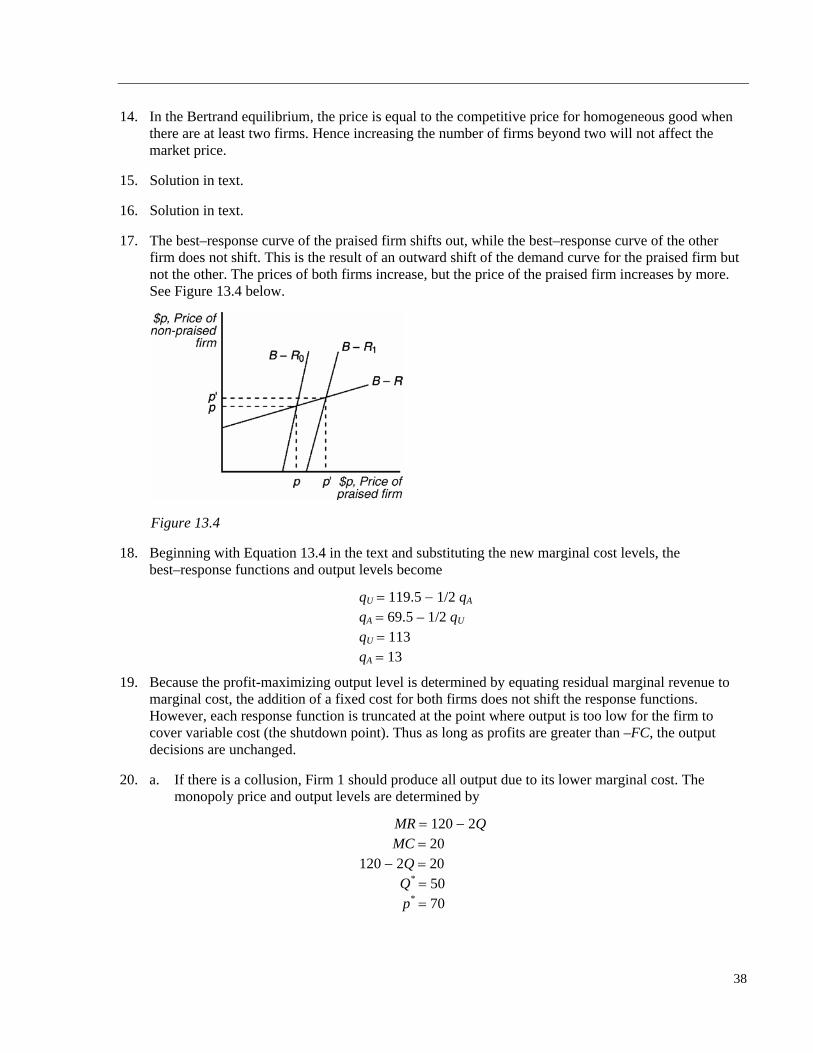
17. The best–response curve of the praised firm shifts out, while the best–response curve of the other firm does not shift. This is the result of an outward shift of the demand curve for the praised firm but not the other. The prices of both firms increase, but the price of the praised firm increases by more. See Figure 13.4 below.

Figure 13.4

18. Beginning with Equation 13.4 in the text and substituting the new marginal cost levels, the best–response functions and output levels become

qU 119.5 1/2 qA qA 69.5 – 1/2 qU

qU 113 qA 13

19. Because the profit-maximizing output level is determined by equating residual marginal revenue to marginal cost, the addition of a fixed cost for both firms does not shift the response functions. However, each response function is truncated at the point where output is too low for the firm to cover variable cost (the shutdown point). Thus as long as profits are greater than –FC, the output decisions are unchanged.

20. a. If there is a collusion, Firm 1 should produce all output due to its lower marginal cost. The monopoly price and output levels are determined by

MR 120 2Q MC 20 120 2Q 20 Q* 50 p* 70

38

b. To calculate the Cournot equilibrium, derive the response function and solve each by setting it equal to the appropriate marginal cost for each firm. Then, solve the response functions simultaneously to determine output.

p 120 q1 q2

1rMR 120 2q1 q2

2rMR 120 q1 2q2

120 2q1 q2 20

q1 50 – 1/2 q2

120 – q1 2q2 40

q2 40 1/2 q1

q1* 40

q2* 20

Q* 60

p* 60


22. The response functions and output levels with the subsidy are

qU 120 1/2qA

qA 120 – 1/2qU

qU qA 80


24. When there are multiple followers instead of one, the response function of the followers becomes

qi (a m)/nb q1/n

The leader maximizes profits taking the best-response functions as given. The output of the leader is the same as the one follower example.

q1 (a m)/2b

Industry output is Q [(a – m)/2b][(2n 1)/n].


26. If marginal cost is equal to zero, we can use the same methodology described above to solve for the new prices. In this case, the response functions are

p1 25 0.25p2

p2 25 0.25p1

and the new equilibrium prices are p1 33.33, p2 33.33.

39

27. This problem is solved using the same methodology as in the previous two problems, except that now, the response functions are asymmetric due to the difference in marginal cost. The best-response functions are

p1 40 0.25p2

p2 30 0.25p1

and the new equilibrium prices are p1 50.67, p2 42.67.











40

238. Firm 1 earns revenue 21 1 1 2 1 1 1 1(1 )R pq q q q q q q q , which corresponds to the marginal

revenue of

11 1

1

1 2R

2MR qq

q

Firm 1 maximizes its profit by satisfying the first order condition (FOC) 1 1MR MC . Due to the government subsidy, the firm faces marginal cost 1MC m s . Hence, the FOC is

. The corresponding response curve is 1 21 2q q m s

21

1 1

2 2

q mq s

(1)

Similarly, Firm 2 maximizes its profit by equating its marginal revenue to its marginal cost. Since Firm 2 receives no subsidy, 2 .MC m Then for Firm 2 we have:

22 2 1 2 2 2 2 1

2 2 1

2 2

2 1

(1 )

1 2

1 2

R 2pq q q q q q q q

MR q q

MR MC

q q m

The reaction function of Firm 2 is

12

1

2

q mq

(2)

Solving Equations 1 and 2 simultaneously, we obtain equilibrium values:

*1

*2

1 2

3 31 1

3 3

mq s

mq s

(3)

The net national income of Government 1 is:

1 1

1 1 1

1 1

1 2 1 1

( )

(1 )

NNI sq

1pq mq sq sq

pq mq

q q q mq

(4)

After substituting Equations 3 into 4 and completing some algebra, we find that

1 2 1

3 3

m s s mNNI

Government 1 maximizes its NNI by solving the FOC:

1 2 1

3 3

1 40

9

m s s mNNI

s s

s m

which suggests that the optimal subsidy is

* 1

4

ms

(5)

Substituting Equation 5 into Equation 3 gives

*1

*2

1

21

4

mq

mq

which are the outputs of the Stackelberg leader and follower respectively (confirm Equation 13.30, p. 465, in the textbook when 1).a b

39. In the Cournot model of Solved Problem 13.3, a subsidy causes the best-response function of Firm 1 to shift outward.


41

42

Ch14

1.In each panel, the dominant strategy for each firm is to advertise. This implies that pairs advertise-advertise are Nash equilibria in both panels of Table 14.4.


3. Assume you’re Lori. If Max works, your best strategy is to give no bonus (your payoff is 3), rather than give a bonus (your payoff is 1). If Max loafs, again, your best strategy is to give no bonus (your payoff is 0), rather than give a bonus (your payoff is 1). Hence, “No Bonus” is Lori’s dominant strategy. Now assume you’re Max. If Lori offers you a bonus, your best strategy is to loaf because the payoff is 3, rather than 2 when you work. If Lori gives no bonus, again, your best strategy is to loaf (payoff of 0 vs. payoff of 1 if you work). This means that “Loaf” is Max’s dominant strategy. Combining two dominant strategies together suggests that the pair No Bonus – Loaf is the Nash equilibrium outcome of this static game.

4. a. There are two Nash equilibria (the off diagonals). If either firm produces 20 while the other produces 10, neither player has an incentive to change strategies given the strategy of the other player.

b. If Firm 1 can choose first, it will commit to selling 10 units, and Firm 2 sells 20 units. If Firm 1 were to choose 20 units, Firm 2 would choose to produce 10 units, reducing Firm 1’s payoff by $10.

c. If Firm 2 can choose first, it will sell 10 units, and Firm 1 will sell 20. If Firm 2 were to produce 20 units, Firm 1 would produce only 10, reducing Firm 2’s payoff by $25.

5. a. If both must move simultaneously, neither has a dominant strategy because neither can credibly commit to producing the television.

b. The two Nash equilibria are on the off diagonals where one firm enters and the other does not. c. With the subsidy, Zenith can credibly commit to entering the market, because the worst it can do

is to gain 10 if Panasonic also enters. In this case, Zenith will enter and Panasonic will not. d. The equilibrium with the head start is the same as that with the subsidy. Once Zenith commits to

producing the new product, there is no benefit to Panasonic if Panasonic produces it also.

6. There are no pure-strategy Nash equilibria in this game. In each cell, one of the players always would prefer to switch, given the move of the other.

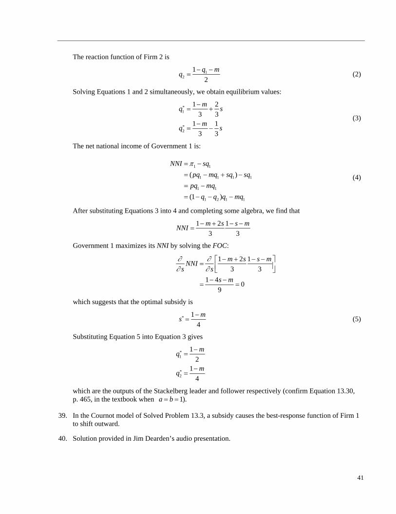
7. The incumbent must compare the two-period profits under two scenarios. In the first scenario, the incumbent overproduces in the first period in order to reduce marginal cost in the second period, knowing that it will be a monopolist in the second period. In the second scenario, the incumbent produces the profit-maximizing output level in the first period, resulting in duopoly profits (with higher marginal cost) in the second period. In the first game tree below, the monopolist overproduces in the first period, resulting in total profits of $1000, which exceeds the profits with profit-maximizing production in the first period. In the second game tree, profits are greater if the incumbent does not overproduce in the first period.

8. Given the information, an optimal strategy for the rulers may be: (i) spend little resource in catapult research and development; (ii) buy latest technology from other countries; (iii) publicly announce the deployment of catapult. Suppose catapult research and development required a substantial fixed cost, this strategy is particularly suitable for small countries. Since new technology was not well protected, public announcement of research and development would encourage free riding of other countries. On the other hand, credible announcement of catapult deployment would help to discourage possible attacks.



11. The advertising might be strategic to increase Microsoft’s own market share by attracting customers from competitors. On the other hand, it does not necessarily reflect its “fear” of competitors. The advertising might target new customers. Overall, the optimal advertising is determined jointly by the marginal cost and marginal benefit.

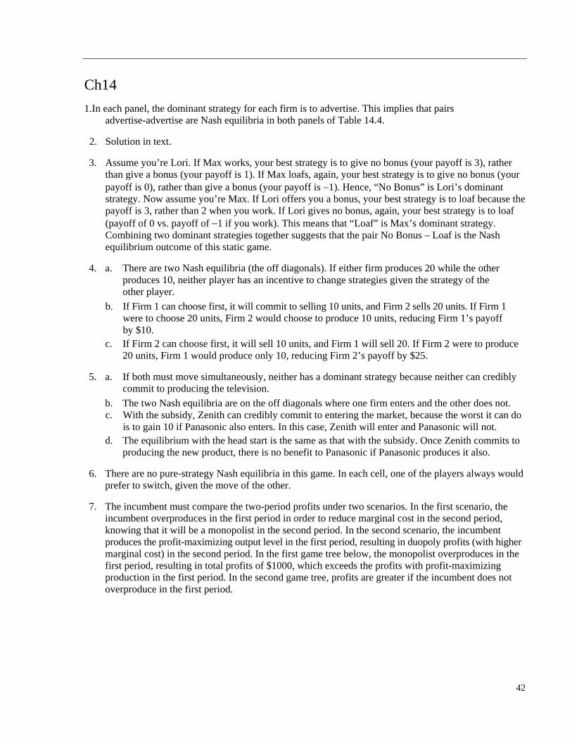
12. Figure 14.1a offers an extensive form representation of the sequential game when Mimi moves first. Using backward induction we conclude that Jeff will not choose actions that are double-crossed because alternatives offer Jeff better payoffs (4 vs. 2 and 1 vs. 0). Given Jeff’s preferred actions, Mimi receives the same payoff of 1 regardless of what she does. Since supporting Jeff will not improve Mimi’s payoff, she may choose not to support him.

If Jeff moves first, the game looks as in Figure 14.1b. When Mimi makes a decision, she chooses actions that give her the highest payoffs; we crossed actions that Mimi will not choose. Then Jeff realizes that if he looks for a job, his payoff will be 2, and if he does not, his payoff will be 0. Maximizing his payoff, Jeff chooses to look for a job. This means that the subgame perfect Nash equilibrium is the strategy look-support with the outcome of (4, 2).

43

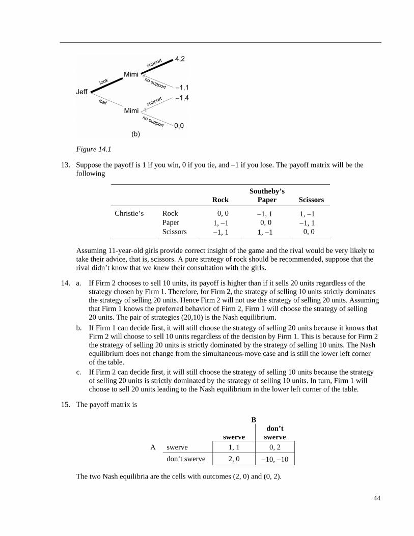
Figure 14.1

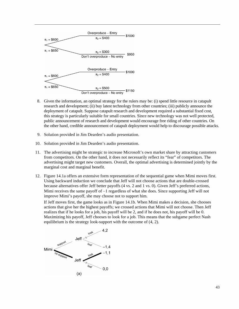
13. Suppose the payoff is 1 if you win, 0 if you tie, and 1 if you lose. The payoff matrix will be the following

Southeby’s

Rock Paper Scissors

Christie’s Rock 0, 0 1, 1 1, 1 Paper 1, 1 0, 0 1, 1 Scissors 1, 1 1, 1 0, 0

Assuming 11-year-old girls provide correct insight of the game and the rival would be very likely to take their advice, that is, scissors. A pure strategy of rock should be recommended, suppose that the rival didn’t know that we knew their consultation with the girls.

14. a. If Firm 2 chooses to sell 10 units, its payoff is higher than if it sells 20 units regardless of the strategy chosen by Firm 1. Therefore, for Firm 2, the strategy of selling 10 units strictly dominates the strategy of selling 20 units. Hence Firm 2 will not use the strategy of selling 20 units. Assuming that Firm 1 knows the preferred behavior of Firm 2, Firm 1 will choose the strategy of selling 20 units. The pair of strategies (20,10) is the Nash equilibrium.

b. If Firm 1 can decide first, it will still choose the strategy of selling 20 units because it knows that Firm 2 will choose to sell 10 units regardless of the decision by Firm 1. This is because for Firm 2 the strategy of selling 20 units is strictly dominated by the strategy of selling 10 units. The Nash equilibrium does not change from the simultaneous-move case and is still the lower left corner of the table.

c. If Firm 2 can decide first, it will still choose the strategy of selling 10 units because the strategy of selling 20 units is strictly dominated by the strategy of selling 10 units. In turn, Firm 1 will choose to sell 20 units leading to the Nash equilibrium in the lower left corner of the table.

15. The payoff matrix is

B

swerve don’t

swerve swerve 1, 1 0, 2 A

don’t swerve 2, 0 10, 10

The two Nash equilibria are the cells with outcomes (2, 0) and (0, 2).

44

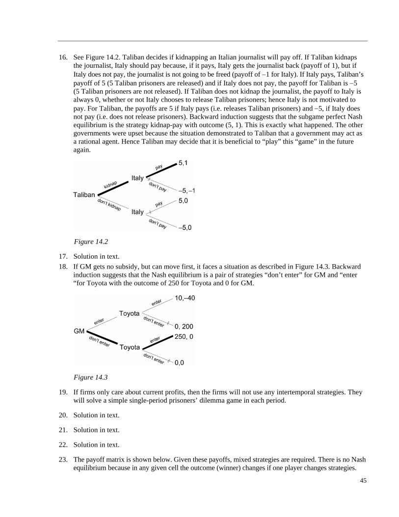
16. See Figure 14.2. Taliban decides if kidnapping an Italian journalist will pay off. If Taliban kidnaps the journalist, Italy should pay because, if it pays, Italy gets the journalist back (payoff of 1), but if Italy does not pay, the journalist is not going to be freed (payoff of 1 for Italy). If Italy pays, Taliban’s payoff of 5 (5 Taliban prisoners are released) and if Italy does not pay, the payoff for Taliban is 5 (5 Taliban prisoners are not released). If Taliban does not kidnap the journalist, the payoff to Italy is always 0, whether or not Italy chooses to release Taliban prisoners; hence Italy is not motivated to pay. For Taliban, the payoffs are 5 if Italy pays (i.e. releases Taliban prisoners) and 5, if Italy does not pay (i.e. does not release prisoners). Backward induction suggests that the subgame perfect Nash equilibrium is the strategy kidnap-pay with outcome (5, 1). This is exactly what happened. The other governments were upset because the situation demonstrated to Taliban that a government may act as a rational agent. Hence Taliban may decide that it is beneficial to “play” this “game” in the future again.

Figure 14.2


18. If GM gets no subsidy, but can move first, it faces a situation as described in Figure 14.3. Backward induction suggests that the Nash equilibrium is a pair of strategies “don’t enter” for GM and “enter “for Toyota with the outcome of 250 for Toyota and 0 for GM.

Figure 14.3

19. If firms only care about current profits, then the firms will not use any intertemporal strategies. They will solve a simple single-period prisoners’ dilemma game in each period.




23. The payoff matrix is shown below. Given these payoffs, mixed strategies are required. There is no Nash equilibrium because in any given cell the outcome (winner) changes if one player changes strategies.

45

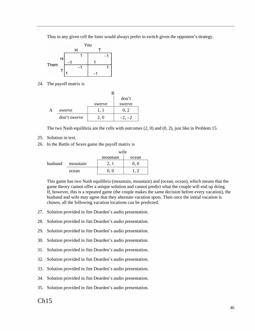
Thus in any given cell the loser would always prefer to switch given the opponent’s strategy.

24. The payoff matrix is

B

swerve don’t

swerve swerve 1, 1 0, 2 A

don’t swerve 2, 0 2, 2

The two Nash equilibria are the cells with outcomes (2, 0) and (0, 2), just like in Problem 15.


26. In the Battle of Sexes game the payoff matrix is

wife mountain ocean

mountain 2, 1 0, 0 husband

ocean 0, 0 1, 2

This game has two Nash equilibria (mountain, mountain) and (ocean, ocean), which means that the game theory cannot offer a unique solution and cannot predict what the couple will end up doing. If, however, this is a repeated game (the couple makes the same decision before every vacation), the husband and wife may agree that they alternate vacation spots. Then once the initial vacation is chosen, all the following vacation locations can be predicted.










46

Ch15

1.The competitive firm’s demand curve for labor is given by the equation w MRPL p MPL. Because price is constant, when marginal product is rising, the demand curve for labor slopes upward (the firm will continue to hire labor throughout this stage). When marginal product is negative, demand for labor is negative (the firm will reduce labor).


3. There are two opposing effects. With a change in relative factor prices, a firm that can easily substitute capital for labor will do so, which has a negative effect on the demand for labor. However, when the cost of capital falls, the firm’s demand for labor typically increases in the long run because with less expensive capital, the firm can profitably expand output (i.e., if inputs are complementary). In either case, the long-run demand curve for labor is more elastic than the short run curve.

4. With the entry of a second firm and a resulting Cournot equilibrium, the demand curve of the dominant firm shifts to the left. Accordingly, its labor demand curve also shifts to the left.

5. If the labor supply curve is horizontal, the effect is the same in either case. If it is positively sloped, the effect is larger if the output market is monopolistic. Because price is larger than marginal revenue for a monopolist, marginal revenue product curves lie to the left and are steeper (less elastic) than value of marginal product curves. When the labor supply curve shifts, the quantity of labor changes by less, but the wage changes more than if the market were competitive.

6. In the short run capital is fixed. The monopolist sets w MRPL. When L K, MPL 0. Thus no workers are hired beyond this point. When L K, MPL is positive, the firm hires labor until w MRPL.

7. The monopsonist will advertise if the increase in pre-advertising expense profits exceed $1000. This occurs if the advertisement causes the wage bill to fall by more than $1000. The ad causes the wage and marginal expense for labor to fall. Marginal cost for the firm is reduced, and employment of that input increases, as does output. The marginal revenue product of the additional output must exceed the marginal expense of the input, plus the cost of the advertisement.

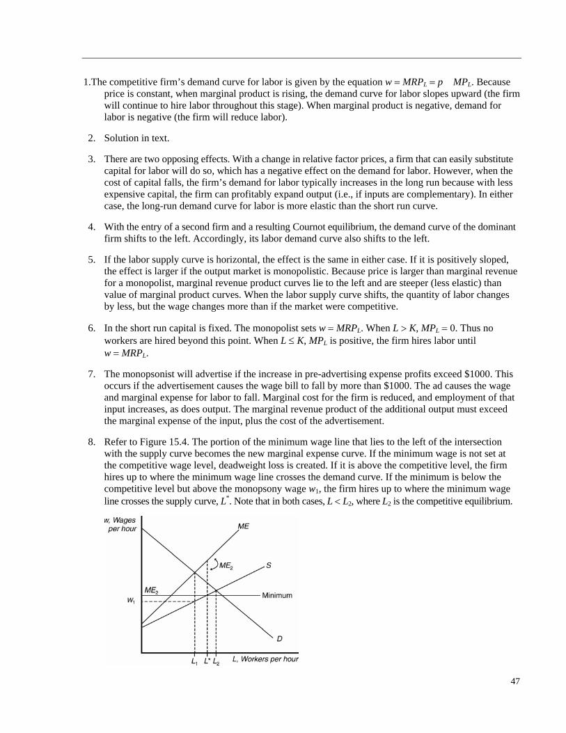
8. Refer to Figure 15.4. The portion of the minimum wage line that lies to the left of the intersection with the supply curve becomes the new marginal expense curve. If the minimum wage is not set at the competitive wage level, deadweight loss is created. If it is above the competitive level, the firm hires up to where the minimum wage line crosses the demand curve. If the minimum is below the competitive level but above the monopsony wage w1, the firm hires up to where the minimum wage line crosses the supply curve, L*. Note that in both cases, L L2, where L2 is the competitive equilibrium.

47

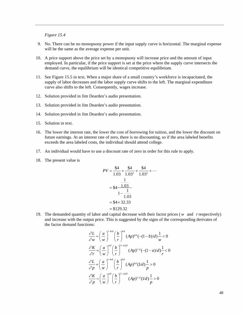
Figure 15.4

9. No. There can be no monopsony power if the input supply curve is horizontal. The marginal expense will be the same as the average expense per unit.

10. A price support above the price set by a monopsony will increase price and the amount of input employed. In particular, if the price support is set at the price where the supply curve intersects the demand curve, the equilibrium will be identical competitive equilibrium.

11. See Figure 15.5 in text. When a major share of a small country’s workforce is incapacitated, the supply of labor decreases and the labor supply curve shifts to the left. The marginal expenditure curve also shifts to the left. Consequently, wages increase.





16. The lower the interest rate, the lower the cost of borrowing for tuition, and the lower the discount on future earnings. At an interest rate of zero, there is no discounting, so if the area labeled benefits exceeds the area labeled costs, the individual should attend college.

17. An individual would have to use a discount rate of zero in order for this rule to apply.

18. The present value is

2 3

$4 $4 $4

1.03 1.03 1.031

1.03$41

11.03

$4 32.33

$129.32

PV

19. The demanded quantity of labor and capital decrease with their factor prices ( and respectively) and increase with the output price. This is suggested by the signs of the corresponding derivates of the factor demand functions:

w r

1 / /

1/

/ 1 /

1/

1 / /

1/

/ 1 /

1/

1( ) ( (1 )/ ) 0

1( ) ( (1 )/ ) 0

1( ) (1/ ) 0

1( ) (1/ ) 0

b d b d

d

a d a d

d

b d b d

d

a d a d

d

L a bAp b d

w w r w

K a bAp a d

r w r r

L a bAp d

p w r p

K a bAp d

p w r p

48

20. The marginal product of labor is 0.2L0.8K0.3. Suppose the marginal revenue is MR, then the marginal revenue product MRPL MR * 0.2L0.8K0.3.


22. Yes. In the production function given, labor and capital are perfect substitutes. The firm will produce using whichever input is cheaper. Long-run average cost will equal marginal cost (min{w, r}). Thus firm size is indeterminate.

23. An example of a constant elasticity demand curve is p AQb. Marginal revenue product of labor is defined as .L LMRP MR MP Then

MPL aQ/L MR (b 1)Aqb

MRPL (aQ/L)[(b 1)AQb].

24. To get the marginal expenditure curve, multiply the supply curve by Q, then take the derivative with respect to Q. ME 10 2Q.

25. The firm sets marginal revenue equal to marginal expenditure.

10 2Q 50 – 2Q Q* 10 p* 40.

The competitive equilibrium is Q 20, p 30, obtained by setting supply equal to demand (10 Q 50 – Q).


27. The present value is $285.93 100 100/1.05 100/1.052.

28. A principal of $2000 would earn $200 in interest per year at 10% compounded annually.

29. The present value is PV [100/(1 i)] (100/(1 i)2.

30. Whether you should buy or rent depends on how long you believe the phone will last and the interest rate. Even if the interest (discount) rate is zero, the phone would have to last 10 years for the payments to be equal. At an interest rate of 10%, the cost is equal only if the phone lasts forever. Thus the individual is better off renting.

31. The cost to buy the washer now is $800. If we don’t buy the washer now, the present discounted value of 5 years’ higher operating cost by using the older washer (assuming they are realized at year-end) and buying the washer 5 years later (assuming the price is the same) is:PV 80[1/(1.05)1 1/(1.05)2 · · · 1/(1.05)5] 800/(1.05)5 $346.66 626.82 973.48 800. So the washer should be purchased.

32. The resale value of the refrigerator today is worth $90.70 100/(1 i)2. Subtracting this from the $200 purchase price yields a net price of $109.30.

33. The question is whether saving $10 per year for 10 years is worth $100 now (the difference in the prices of the machines). Given that the total savings over the ten-year period is just $100, any interest rate above zero would make the more expensive machine a bad choice.

49


35. The price of oil would have to be more than p(1 i).

36. In the first period,

p1

1/

[1 (1 2)]A

Q

p2 p1(1 i).

37. Using Equation 15.21 gives a close approximation of the precise answer, which would be derived from Equation 15.20 (if you want to try this, I suggest either a finance calculator, or Excel). The breakeven discount rate is approximately 16%. Because most of the enlisted men took the cash, they are implicitly discounting at a rate greater than that. Officers are about evenly divided.

38. Thirty–seven days per year is about 1/10 of a year. Thus they earn about one-tenth of the APR or 4% per year on the value of input purchases. For every million dollars spent on inputs, they save $4000.

39. Using Equation 15.18, the value of the stock at 5% per year is $21,609.71 in 30 years. At 4.75% it is $20,118.28. Thus, Alex will accumulate $1491.43 more than Spencer.


41. As was shown in Solved Problem 15.4, the present value of the expected returns is $196.7 million. If the purchase price is $205 million, it is not worth to buy it.

42. The internal rate of return is 20/400 0.05.

43 Solution in text.




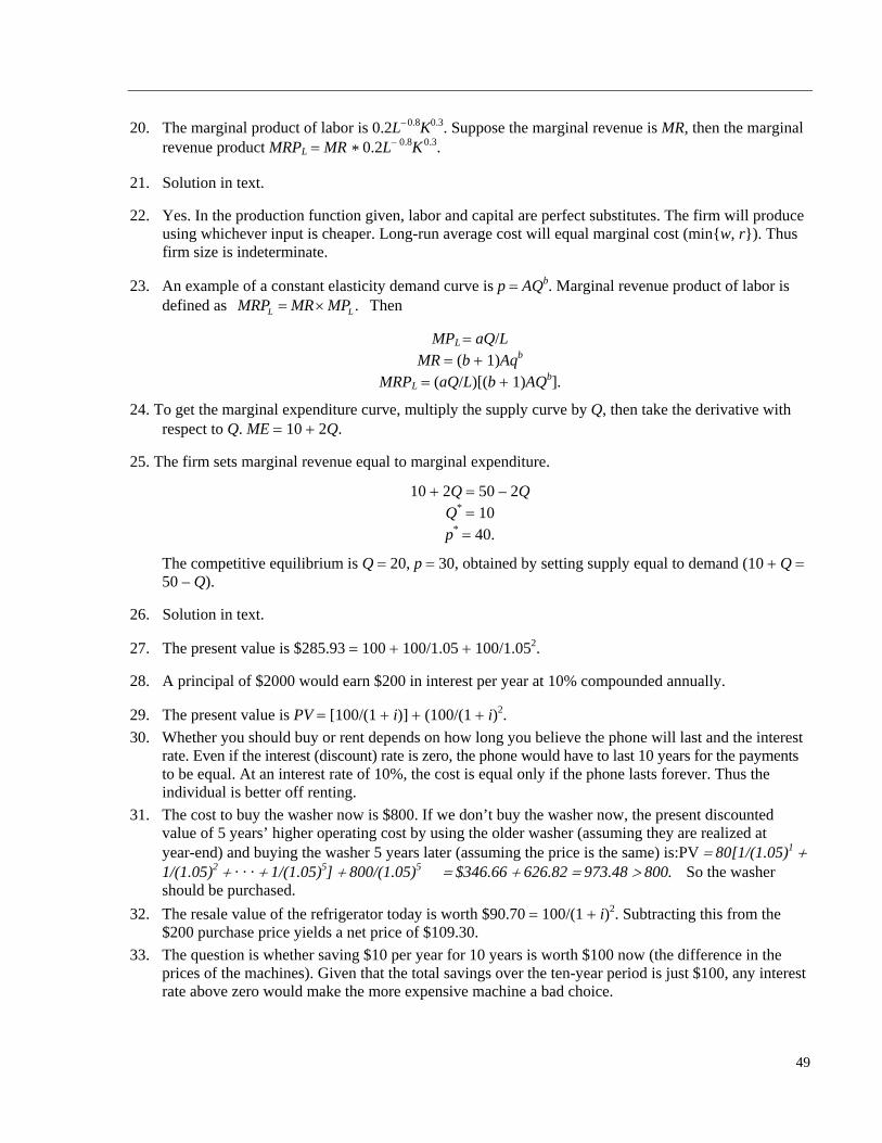
47. See Figure 15.5. Suppose the value of the good goes up first then decreases as shown in the figure. The two upward sloping curves represent present value of the good if it was sold this year with different interest rate. The optimal harvest time is the time when the gap between the value of the good and the present value of the good if it was sold this year. As one can tell from the figure, the higher is the interest rate, the earlier is the optimal harvest time (T1 as shown in the figure). If the interest rate is zero, then the optimal harvest time is when the value curve reaches its peak.

50

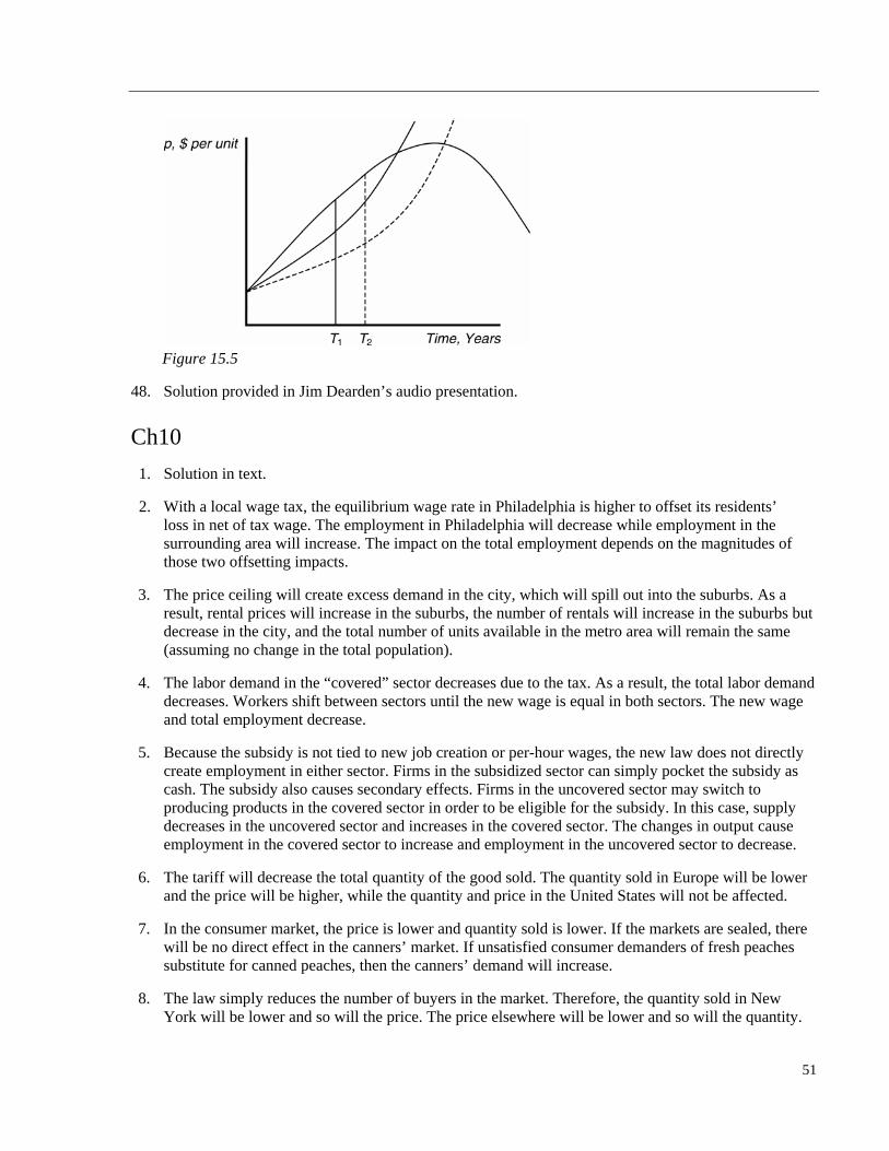
Figure 15.5


Ch10


2. With a local wage tax, the equilibrium wage rate in Philadelphia is higher to offset its residents’ loss in net of tax wage. The employment in Philadelphia will decrease while employment in the surrounding area will increase. The impact on the total employment depends on the magnitudes of those two offsetting impacts.

3. The price ceiling will create excess demand in the city, which will spill out into the suburbs. As a result, rental prices will increase in the suburbs, the number of rentals will increase in the suburbs but decrease in the city, and the total number of units available in the metro area will remain the same (assuming no change in the total population).

4. The labor demand in the “covered” sector decreases due to the tax. As a result, the total labor demand decreases. Workers shift between sectors until the new wage is equal in both sectors. The new wage and total employment decrease.

5. Because the subsidy is not tied to new job creation or per-hour wages, the new law does not directly create employment in either sector. Firms in the subsidized sector can simply pocket the subsidy as cash. The subsidy also causes secondary effects. Firms in the uncovered sector may switch to producing products in the covered sector in order to be eligible for the subsidy. In this case, supply decreases in the uncovered sector and increases in the covered sector. The changes in output cause employment in the covered sector to increase and employment in the uncovered sector to decrease.

6. The tariff will decrease the total quantity of the good sold. The quantity sold in Europe will be lower and the price will be higher, while the quantity and price in the United States will not be affected.

7. In the consumer market, the price is lower and quantity sold is lower. If the markets are sealed, there will be no direct effect in the canners’ market. If unsatisfied consumer demanders of fresh peaches substitute for canned peaches, then the canners’ demand will increase.

8. The law simply reduces the number of buyers in the market. Therefore, the quantity sold in New York will be lower and so will the price. The price elsewhere will be lower and so will the quantity.

51

9. The price in the foreign market will be higher while the quantity sold will be lower. On the other hand, the price in the home country will be lower and quantity sold will be higher, assuming total production remains the same.

10. See Figure 10.4

Figure 10.4


12. Yes, they may want to trade. If two individuals are consuming different bundles and have identical preferences, their marginal rates of substitution may be unequal and they may gain by trading. For example, if each had the utility function U XY, an initial allocation of 4X, 2Y for one person and 2X, 4Y for the other, each would have a utility level of 8, and their marginal rates of substitution would differ. By trading 1 unit of X for 1 unit of Y, each can achieve a utility level of 9.

13. See Figure 10.5. At point A, the individual’s indifference curves are tangent. At point B, however, Joe is indifferent to point A, but Mary is happier, making the allocation implied by B Pareto-superior to that at A.

Figure 10.5

52

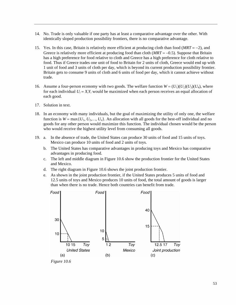
14. No. Trade is only valuable if one party has at least a comparative advantage over the other. With identically sloped production possibility frontiers, there is no comparative advantage.

15. Yes. In this case, Britain is relatively more efficient at producing cloth than food (MRT 2), and Greece is relatively more efficient at producing food than cloth (MRT –0.5). Suppose that Britain has a high preference for food relative to cloth and Greece has a high preference for cloth relative to food. Thus if Greece trades one unit of food to Britain for 2 units of cloth, Greece would end up with 1 unit of food and 3 units of cloth per day, which is beyond its current production possibility frontier. Britain gets to consume 9 units of cloth and 6 units of food per day, which it cannot achieve without trade.

16. Assume a four-person economy with two goods. The welfare function W (U1)(U2)(U3)(U4), where for each individual Ui XiYi would be maximized when each person receives an equal allocation of each good.


18. In an economy with many individuals, but the goal of maximizing the utility of only one, the welfare function is W max{U1, U2,…, Un}. An allocation with all goods for the best-off individual and no goods for any other person would maximize this function. The individual chosen would be the person who would receive the highest utility level from consuming all goods.

19. a. In the absence of trade, the United States can produce 30 units of food and 15 units of toys. Mexico can produce 10 units of food and 2 units of toys.

b. The United States has comparative advantages in producing toys and Mexico has comparative advantages in producing food.

c. The left and middle diagram in Figure 10.6 show the production frontier for the United States and Mexico.

d. The right diagram in Figure 10.6 shows the joint production frontier. e. As shown in the joint production frontier, if the United States produces 5 units of food and

12.5 units of toys and Mexico produces 10 units of food, the total amount of goods is larger than when there is no trade. Hence both countries can benefit from trade.

Figure 10.6

53

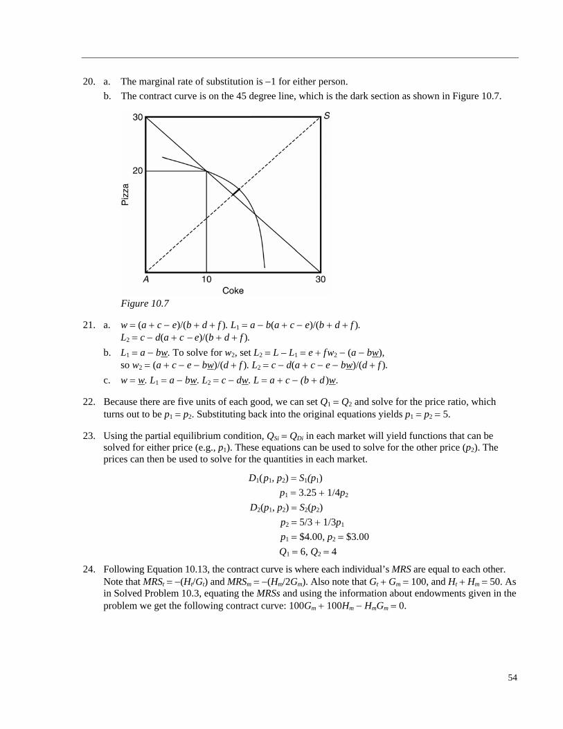
20. a. The marginal rate of substitution is 1 for either person.

b. The contract curve is on the 45 degree line, which is the dark section as shown in Figure 10.7.

Figure 10.7

21. a. w (a c e)/(b d f ). L1 a b(a c e)/(b d f ). L2 c d(a c e)/(b d f ).

b. L1 a bw. To solve for w2, set L2 L – L1 e fw2 (a bw), so w2 (a c e bw)/(d f ). L2 c d(a c e bw)/(d f ).

c. w w. L1 a bw. L2 c dw. L a c (b d)w.

22. Because there are five units of each good, we can set Q1 Q2 and solve for the price ratio, which turns out to be p1 p2. Substituting back into the original equations yields p1 p2 5.

23. Using the partial equilibrium condition, QSi QDi in each market will yield functions that can be solved for either price (e.g., p1). These equations can be used to solve for the other price (p2). The prices can then be used to solve for the quantities in each market.

D1(p1, p2) S1(p1)

p1 3.25 1/4p2

D2(p1, p2) S2(p2)

p2 5/3 1/3p1

p1 $4.00, p2 $3.00

Q1 6, Q2 4

24. Following Equation 10.13, the contract curve is where each individual’s MRS are equal to each other. Note that MRSt (Ht/Gt) and MRSm (Hm/2Gm). Also note that Gt Gm 100, and Ht Hm 50. As in Solved Problem 10.3, equating the MRSs and using the information about endowments given in the problem we get the following contract curve: 100Gm 100Hm HmGm 0.

54

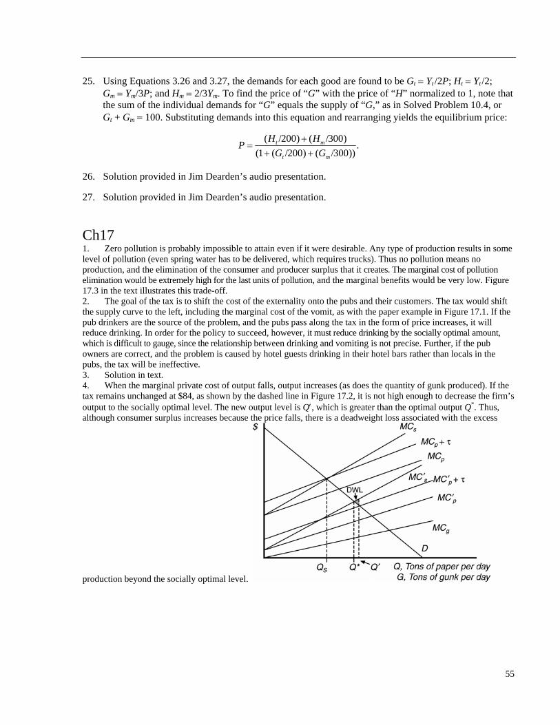
25. Using Equations 3.26 and 3.27, the demands for each good are found to be Gt Yt /2P; Ht Yt /2; Gm Ym/3P; and Hm 2/3Ym. To find the price of “G” with the price of “H” normalized to 1, note that the sum of the individual demands for “G” equals the supply of “G,” as in Solved Problem 10.4, or Gt + Gm 100. Substituting demands into this equation and rearranging yields the equilibrium price:

( /200) ( /300).

(1 ( /200) ( /300))t m

t m

H HP

G G



Ch17 1. Zero pollution is probably impossible to attain even if it were desirable. Any type of production results in some level of pollution (even spring water has to be delivered, which requires trucks). Thus no pollution means no production, and the elimination of the consumer and producer surplus that it creates. The marginal cost of pollution elimination would be extremely high for the last units of pollution, and the marginal benefits would be very low. Figure 17.3 in the text illustrates this trade-off. 2. The goal of the tax is to shift the cost of the externality onto the pubs and their customers. The tax would shift the supply curve to the left, including the marginal cost of the vomit, as with the paper example in Figure 17.1. If the pub drinkers are the source of the problem, and the pubs pass along the tax in the form of price increases, it will reduce drinking. In order for the policy to succeed, however, it must reduce drinking by the socially optimal amount, which is difficult to gauge, since the relationship between drinking and vomiting is not precise. Further, if the pub owners are correct, and the problem is caused by hotel guests drinking in their hotel bars rather than locals in the pubs, the tax will be ineffective. 3. Solution in text. 4. When the marginal private cost of output falls, output increases (as does the quantity of gunk produced). If the tax remains unchanged at $84, as shown by the dashed line in Figure 17.2, it is not high enough to decrease the firm’s output to the socially optimal level. The new output level is Q, which is greater than the optimal output Q*. Thus, although consumer surplus increases because the price falls, there is a deadweight loss associated with the excess

production beyond the socially optimal level.

55

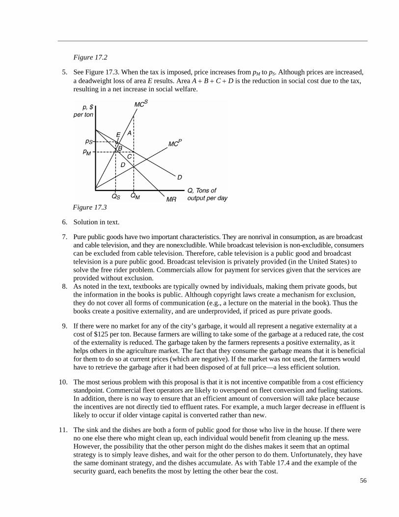
Figure 17.2

5. See Figure 17.3. When the tax is imposed, price increases from pM to pS. Although prices are increased, a deadweight loss of area E results. Area A B C D is the reduction in social cost due to the tax, resulting in a net increase in social welfare.

Figure 17.3


7. Pure public goods have two important characteristics. They are nonrival in consumption, as are broadcast and cable television, and they are nonexcludible. While broadcast television is non-excludible, consumers can be excluded from cable television. Therefore, cable television is a public good and broadcast television is a pure public good. Broadcast television is privately provided (in the United States) to solve the free rider problem. Commercials allow for payment for services given that the services are provided without exclusion.

8. As noted in the text, textbooks are typically owned by individuals, making them private goods, but the information in the books is public. Although copyright laws create a mechanism for exclusion, they do not cover all forms of communication (e.g., a lecture on the material in the book). Thus the books create a positive externality, and are underprovided, if priced as pure private goods.

9. If there were no market for any of the city’s garbage, it would all represent a negative externality at a cost of $125 per ton. Because farmers are willing to take some of the garbage at a reduced rate, the cost of the externality is reduced. The garbage taken by the farmers represents a positive externality, as it helps others in the agriculture market. The fact that they consume the garbage means that it is beneficial for them to do so at current prices (which are negative). If the market was not used, the farmers would have to retrieve the garbage after it had been disposed of at full price—a less efficient solution.

10. The most serious problem with this proposal is that it is not incentive compatible from a cost efficiency standpoint. Commercial fleet operators are likely to overspend on fleet conversion and fueling stations. In addition, there is no way to ensure that an efficient amount of conversion will take place because the incentives are not directly tied to effluent rates. For example, a much larger decrease in effluent is likely to occur if older vintage capital is converted rather than new.

11. The sink and the dishes are both a form of public good for those who live in the house. If there were no one else there who might clean up, each individual would benefit from cleaning up the mess. However, the possibility that the other person might do the dishes makes it seem that an optimal strategy is to simply leave dishes, and wait for the other person to do them. Unfortunately, they have the same dominant strategy, and the dishes accumulate. As with Table 17.4 and the example of the security guard, each benefits the most by letting the other bear the cost.

56

12. Because of the negative externality generated by a SUV, the government can impose a SUV tax such that people have to pay more to driving a SUV.

13. Having Michael Jordan in the NBA increased the total revenue of the league and therefore each team benefited. In terms of social welfare, the huge amount of money spent in advertising may be a social waste.

14. Those games and movies are not designed to impact people’s productivity in any way. However, the firms do not control their employees’ after-work activity, although they clearly affect people’s work performance. If we consider these examples a negative externality, we might as well label all holidays the same way.

15. Since the marginal benefit is significantly higher than marginal cost, the industry advertising is actually not optimal.

16. Using the information in Figure 17.6 in the text. At the market price of guard service of $10 per hour, the TV store will hire four guards and the ice-cream store will hire none. Now with a $2 per hour subsidy from the mall owner, the private price of the TV store will be $8 per hour. Subsequently, the TV store will hire 5 guards, which makes the social marginal benefit equal to social marginal cost and therefore achieves social optimal.






22. a. The unregulated equilibrium (MCP p) is Q 60, p 140.

b. The socially optimal equilibrium (MCS MCP MCg p) is Q 40, p 160. A specific tax of $40 per unit results in this outcome. With the tax, MCP 120 Q.

c. The unregulated monopoly output is the same as the socially optimal output. Q 40, p 160. d. The monopolist is already producing the socially optimal output level, and thus does not require

regulation.

23. The parameter A must be positive in order for gunk reduction to be beneficial, and must be between zero and 1 in order for marginal benefits of gunk reduction to decline. If costs are increasing at an increasing rate, must be greater than one.

24. To determine this level, set marginal benefit equal to marginal cost.

1 1

( )

1/( )

/( )

[ /( )

AH H

H A

H A

25. To find the social demand for the service, add the demand curves vertically (you must solve for p first). Individual inverted demands are p (–a1/b1) (1/b1)q, and p (–a2/b2) (1/b2)q. When added, the resulting curve will be nonlinear unless the demand curves have the same horizontal axis intercept. Note that b1, b2 0. For the solution below, assume that a1/b1 a2/b2.

57

p (–a1/b1 – a2/b2) (1/b1 1/b2) q if q a1

p (–a2/b2) (1/b2)q if q a1

26. We differentiate the utility function to find that

1

1

11

1 1

1

1

a

a

Ua A B

A

UA

B

Then

11

11

1

1

1 1 11

aU

AaU

B

a A B a BMRS

AA

1

Due to the symmetry of the problem,

2 2

2 2

2

12 2 2

2

U aA

U aB

a A B a BMRS

A A

2

The optimal allocation toward a public good is achieved when Equation 17.5 is satisfied, that is, Then 1 2 1.MRS MRS

1 1 2 2

1 1 2 2

1

.

a B a B

A AA a B a B



58

answers to questions and problems in the...

Documents