ansys tutorial for assignment 2

University of Victoria MECH420 – Finite Element Methods Summer 2012

By: Majid Soleimaninia

Tutorial for Assignment #2 Gantry Crane Analysis

By ANSYS (Mechanical APDL) V.13.0

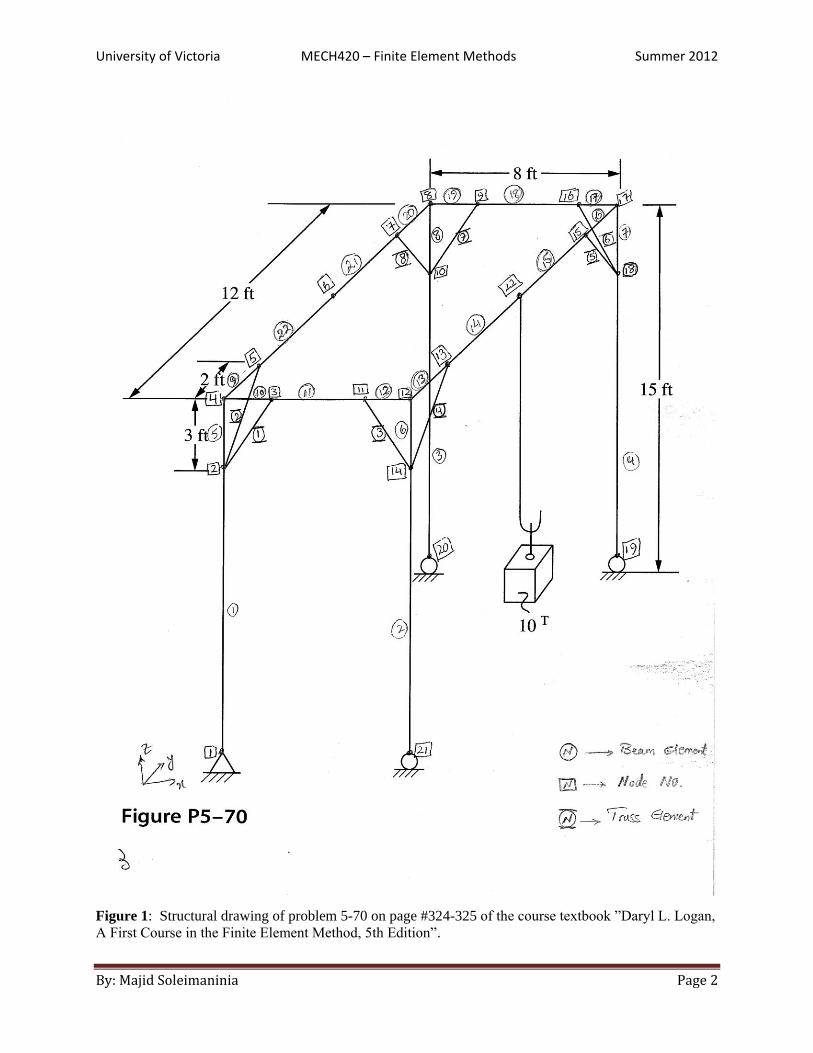
1 Problem Description Design a gantry crane meeting the geometry presented in Figure 1 on page #325 of the course

textbook ”Daryl L. Logan, A First Course in the Finite Element Method, 5th

Edition” (a modified

version of problem 5-70 on page #324-325). Assume that structural steel is used for all the truss

members (ASTM- A36). The design should:

1. be as light as possible,

2. have a beam structure at the top that is well removed from the possibility of material

yield due to bending (using a FOS of 5.0), and

3. have vertical columns that are well removed from the possibility of yield and buckling

due to internal compression (using a FOS of 5.0).

4. have corner braces that are well removed from the possibility of yield and buckling due

to internal compression (using a FOS of 5.0).

You can assume that all joints are welded except the corner braces which are connected to the

columns and beams with idealized spherical joints.

When calculating the threshold for buckling you can use Euler’s buckling formula (which

assumes pinned-pinned conditions).

Using Appendix F (pages #882-907), you can choose from the wide flange sections listed for the

beam elements (one size used for all beams), the rectangular hollow structural sections (HSS) for

the vertical columns (one size used for all columns) and the pipe sections for the corner bracing

(one size used for all braces).

Material properties can be located inside the back cover of the textbook.

1.1 Deliverables: From your simulation results, provide:

1. An ANSYS plot of the undeformed and the deformed space frame. Choose a scaling

factor for the elastic displacements such that they are appreciable in the plot.

2. A table of output values that compares the nodal displacements (translations only) to

those calculated with your MATLAB Code.



Figure 1: Structural drawing of problem 5-70 on page #324-325 of the course textbook ”Daryl L. Logan,

A First Course in the Finite Element Method, 5th Edition”.



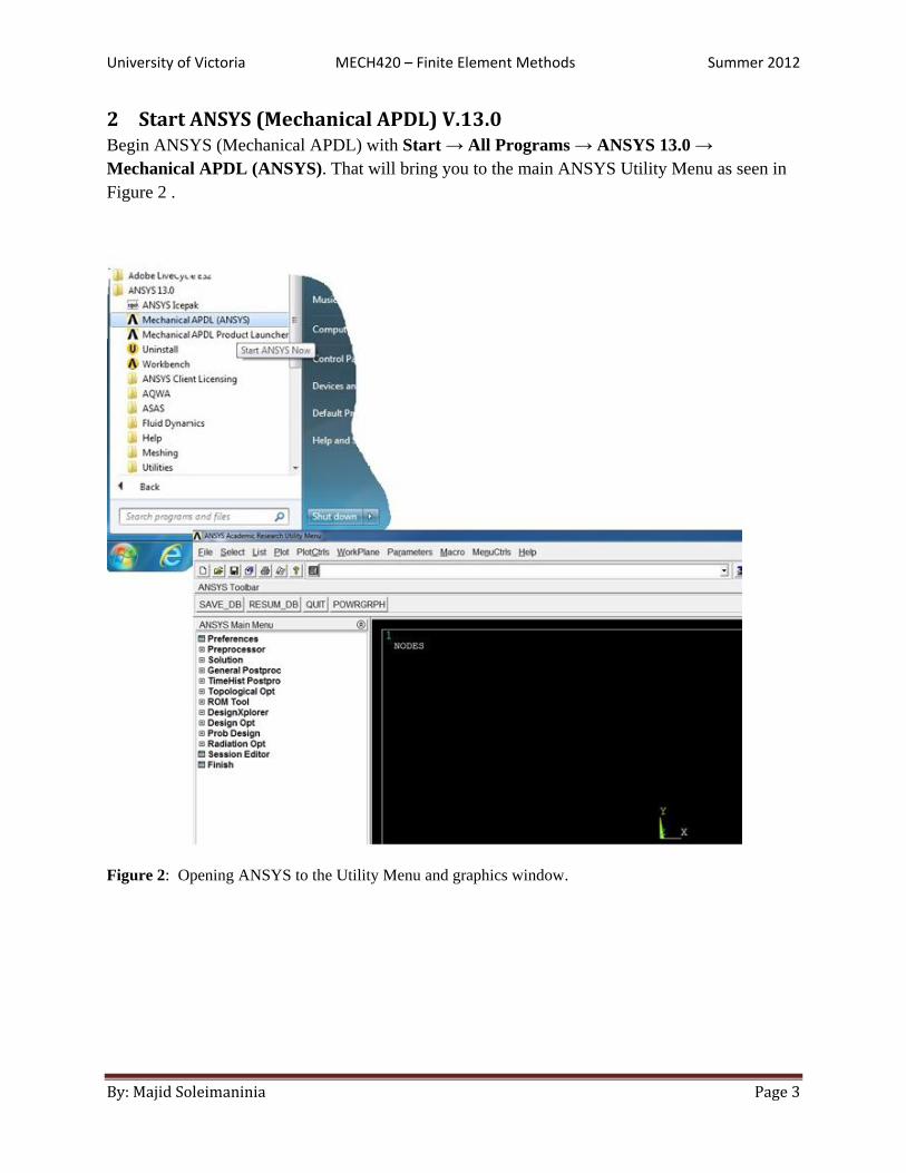
2 Start ANSYS (Mechanical APDL) V.13.0 Begin ANSYS (Mechanical APDL) with Start → All Programs → ANSYS 13.0 →

Mechanical APDL (ANSYS). That will bring you to the main ANSYS Utility Menu as seen in

Figure 2 .

Figure 2: Opening ANSYS to the Utility Menu and graphics window.



3 Preprocessing: Defining the Problem

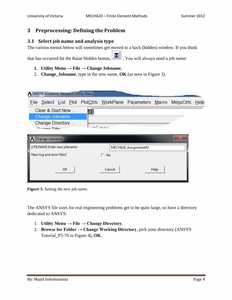
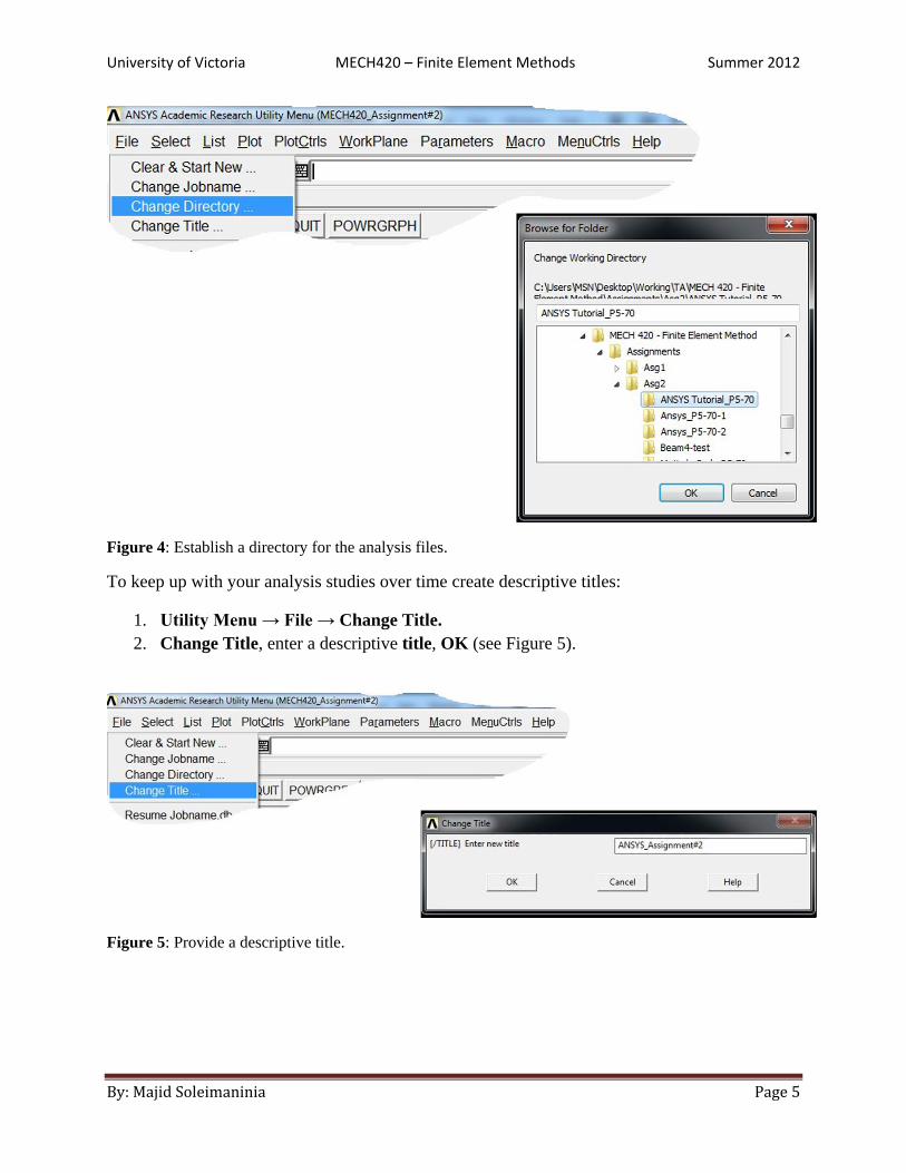
3.1 Select job name and analysis type The various menus below will sometimes get moved to a back (hidden) window. If you think

that has occurred hit the Raise Hidden button, . You will always need a job name:

1. Utility Menu → File → Change Jobname.

2. Change_Jobname, type in the new name, OK (as seen in Figure 3).

The ANSYS file sizes for real engineering problems get to be quite large, so have a directory

dedicated to ANSYS:

1. Utility Menu → File → Change Directory.

2. Browse for Folder → Change Working Directory, pick your directory (ANSYS

Tutorial_P5-70 in Figure 4), OK.

Figure 3: Setting the new job name.



To keep up with your analysis studies over time create descriptive titles:

1. Utility Menu → File → Change Title.

2. Change Title, enter a descriptive title, OK (see Figure 5).

Figure 4: Establish a directory for the analysis files.

Figure 5: Provide a descriptive title.



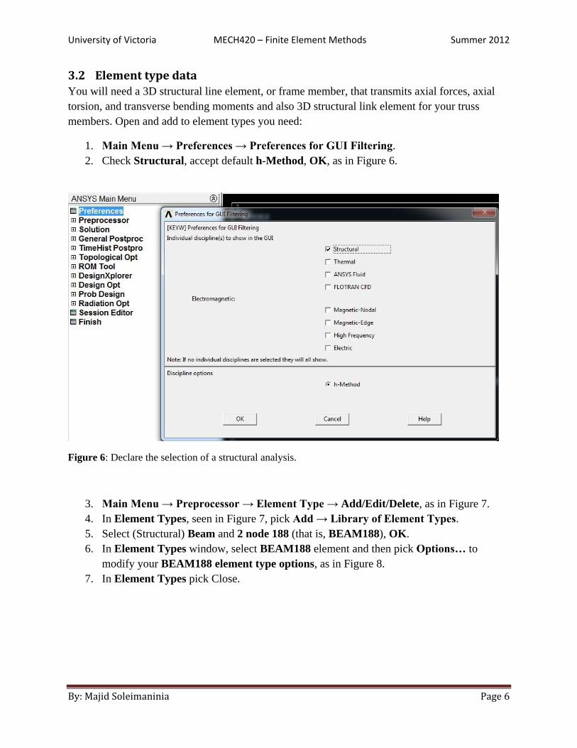
3.2 Element type data

You will need a 3D structural line element, or frame member, that transmits axial forces, axial

torsion, and transverse bending moments and also 3D structural link element for your truss

members. Open and add to element types you need:

1. Main Menu → Preferences → Preferences for GUI Filtering.

2. Check Structural, accept default h-Method, OK, as in Figure 6.

3. Main Menu → Preprocessor → Element Type → Add/Edit/Delete, as in Figure 7.

4. In Element Types, seen in Figure 7, pick Add → Library of Element Types.

5. Select (Structural) Beam and 2 node 188 (that is, BEAM188), OK.

6. In Element Types window, select BEAM188 element and then pick Options… to

modify your BEAM188 element type options, as in Figure 8.

7. In Element Types pick Close.

Figure 6: Declare the selection of a structural analysis.



Now you defined your beam element and need to add truss element as well. In order to add other

elements, open and add to element types you need:

1. Main Menu → Preprocessor → Element Type → Add/Edit/Delete, as in Figure 9.

2. In Element Types, seen in Figure 9, pick Add → Library of Element Types.

3. Select (Structural) Link and 3D finit stn 180 (that is, LINK180), OK.

Figure 7: Select beam element type.

Figure 8: Modify BEAM188 element type options.



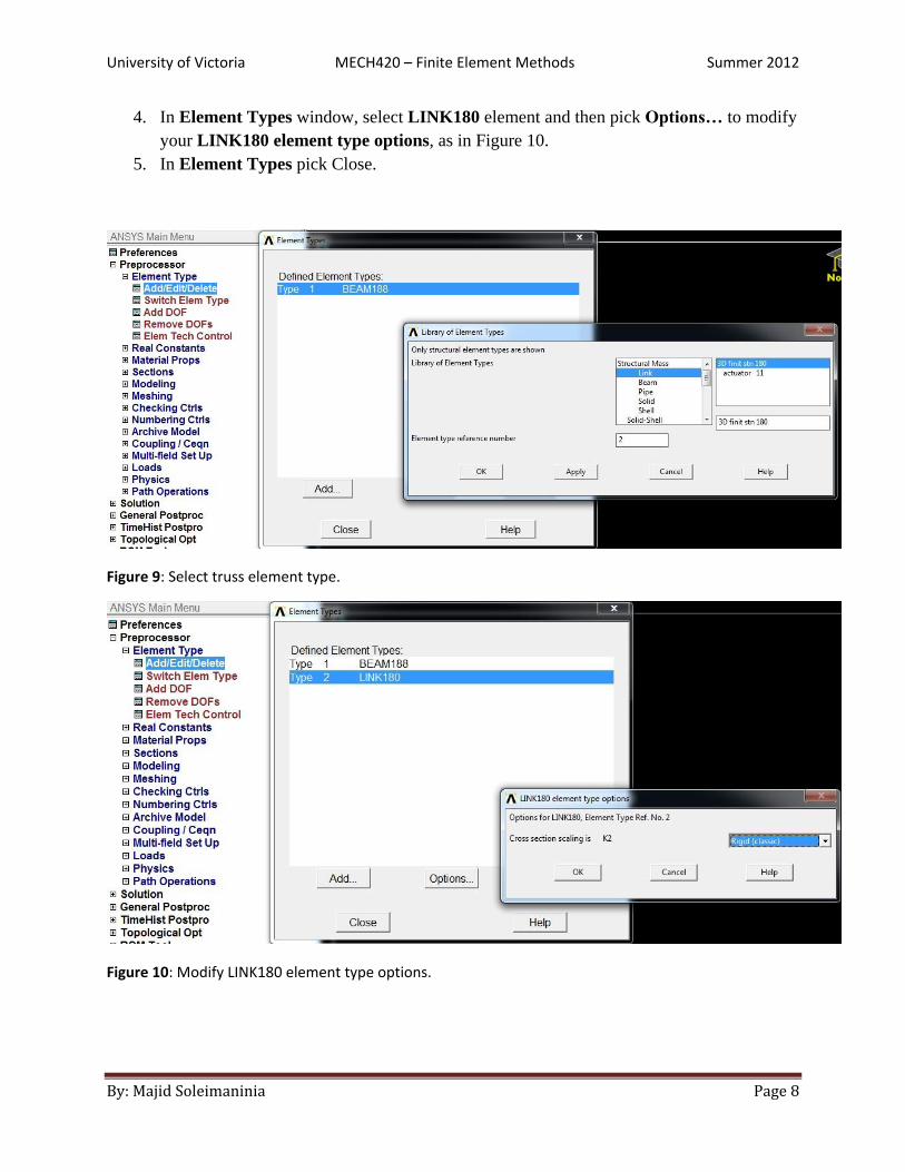
4. In Element Types window, select LINK180 element and then pick Options… to modify

your LINK180 element type options, as in Figure 10.

5. In Element Types pick Close.

Figure 9: Select truss element type.

Figure 10: Modify LINK180 element type options.



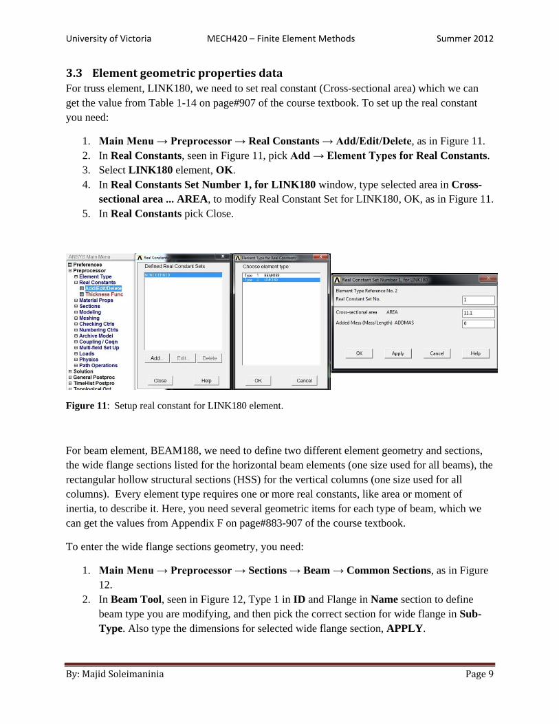
3.3 Element geometric properties data For truss element, LINK180, we need to set real constant (Cross-sectional area) which we can

get the value from Table 1-14 on page#907 of the course textbook. To set up the real constant

you need:

1. Main Menu → Preprocessor → Real Constants → Add/Edit/Delete, as in Figure 11.

2. In Real Constants, seen in Figure 11, pick Add → Element Types for Real Constants.

3. Select LINK180 element, OK.

4. In Real Constants Set Number 1, for LINK180 window, type selected area in Cross-

sectional area ... AREA, to modify Real Constant Set for LINK180, OK, as in Figure 11.

5. In Real Constants pick Close.

For beam element, BEAM188, we need to define two different element geometry and sections,

the wide flange sections listed for the horizontal beam elements (one size used for all beams), the

rectangular hollow structural sections (HSS) for the vertical columns (one size used for all

columns). Every element type requires one or more real constants, like area or moment of

inertia, to describe it. Here, you need several geometric items for each type of beam, which we

can get the values from Appendix F on page#883-907 of the course textbook.

To enter the wide flange sections geometry, you need:

1. Main Menu → Preprocessor → Sections → Beam → Common Sections, as in Figure

12.

2. In Beam Tool, seen in Figure 12, Type 1 in ID and Flange in Name section to define

beam type you are modifying, and then pick the correct section for wide flange in Sub-

Type. Also type the dimensions for selected wide flange section, APPLY.

Figure 11: Setup real constant for LINK180 element.



3. To check your wide flange geometry and dimensions, you can pick Preview in Beam

Tool, as in Figure 12.

4. In Beam Tool pick Close.

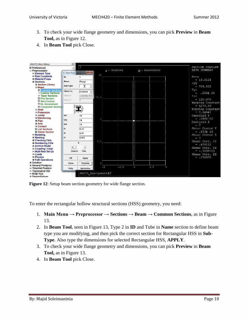
To enter the rectangular hollow structural sections (HSS) geometry, you need:

1. Main Menu → Preprocessor → Sections → Beam → Common Sections, as in Figure

13.

2. In Beam Tool, seen in Figure 13, Type 2 in ID and Tube in Name section to define beam

type you are modifying, and then pick the correct section for Rectangular HSS in Sub-

Type. Also type the dimensions for selected Rectangular HSS, APPLY.

3. To check your wide flange geometry and dimensions, you can pick Preview in Beam

Tool, as in Figure 13.

4. In Beam Tool pick Close.

Figure 12: Setup beam section geometry for wide flange section.



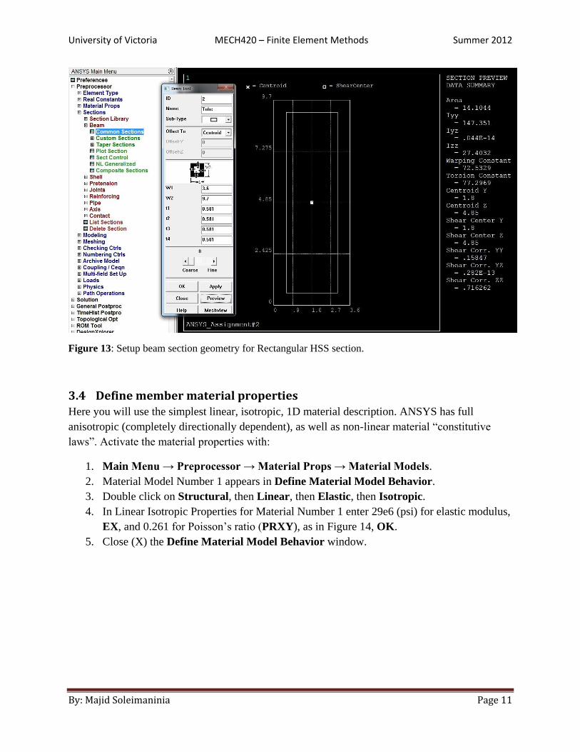
3.4 Define member material properties Here you will use the simplest linear, isotropic, 1D material description. ANSYS has full

anisotropic (completely directionally dependent), as well as non-linear material “constitutive

laws”. Activate the material properties with:

1. Main Menu → Preprocessor → Material Props → Material Models.

2. Material Model Number 1 appears in Define Material Model Behavior.

3. Double click on Structural, then Linear, then Elastic, then Isotropic.

4. In Linear Isotropic Properties for Material Number 1 enter 29e6 (psi) for elastic modulus,

EX, and 0.261 for Poisson’s ratio (PRXY), as in Figure 14, OK.

5. Close (X) the Define Material Model Behavior window.

Figure 13: Setup beam section geometry for Rectangular HSS section.



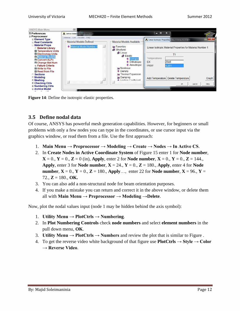
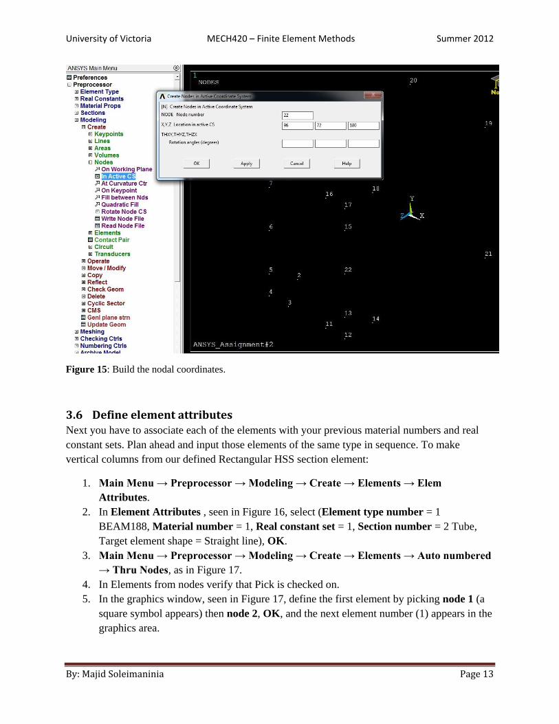
3.5 Define nodal data Of course, ANSYS has powerful mesh generation capabilities. However, for beginners or small

problems with only a few nodes you can type in the coordinates, or use cursor input via the

graphics window, or read them from a file. Use the first approach:

1. Main Menu → Preprocessor → Modeling → Create → Nodes → In Active CS.

2. In Create Nodes in Active Coordinate System of Figure 15 enter 1 for Node number,

X = 0., Y = 0., Z = 0 (in), Apply, enter 2 for Node number, X = 0., Y = 0., Z = 144.,

Apply, enter 3 for Node number, X = 24., Y = 0., Z = 180., Apply, enter 4 for Node

number, X = 0., Y = 0., Z = 180., Apply…, enter 22 for Node number, X = 96., Y =

72., Z = 180., OK.

3. You can also add a non-structural node for beam orientation purposes.

4. If you make a mistake you can return and correct it in the above window, or delete them

all with Main Menu → Preprocessor → Modeling →Delete.

Now, plot the nodal values input (node 1 may be hidden behind the axis symbol):

1. Utility Menu → PlotCtrls → Numbering.

2. In Plot Numbering Controls check node numbers and select element numbers in the

pull down menu, OK.

3. Utility Menu → PlotCtrls → Numbers and review the plot that is similar to Figure .

4. To get the reverse video white background of that figure use PlotCtrls → Style → Color

→ Reverse Video.

Figure 14: Define the isotropic elastic properties.



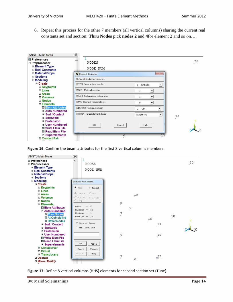
3.6 Define element attributes Next you have to associate each of the elements with your previous material numbers and real

constant sets. Plan ahead and input those elements of the same type in sequence. To make

vertical columns from our defined Rectangular HSS section element:

1. Main Menu → Preprocessor → Modeling → Create → Elements → Elem

Attributes.

2. In Element Attributes , seen in Figure 16, select (Element type number = 1

BEAM188, Material number = 1, Real constant set = 1, Section number = 2 Tube,

Target element shape = Straight line), OK.

3. Main Menu → Preprocessor → Modeling → Create → Elements → Auto numbered

→ Thru Nodes, as in Figure 17.

4. In Elements from nodes verify that Pick is checked on.

5. In the graphics window, seen in Figure 17, define the first element by picking node 1 (a

square symbol appears) then node 2, OK, and the next element number (1) appears in the

graphics area.

Figure 15: Build the nodal coordinates.



6. Repeat this process for the other 7 members (all vertical columns) sharing the current real

constants set and section: Thru Nodes pick nodes 2 and 4for element 2 and so on….

Figure 16: Confirm the beam attributes for the first 8 vertical columns members.

Figure 17: Define 8 vertical columns (HHS) elements for second section set (Tube).



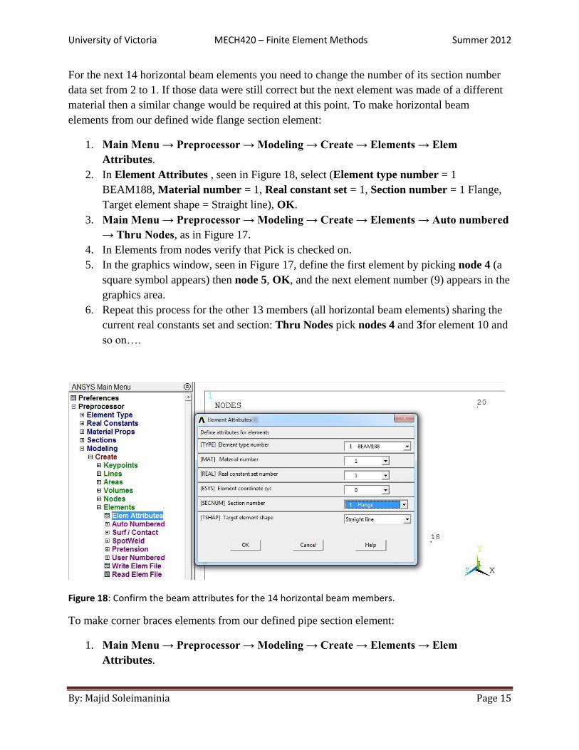
For the next 14 horizontal beam elements you need to change the number of its section number

data set from 2 to 1. If those data were still correct but the next element was made of a different

material then a similar change would be required at this point. To make horizontal beam

elements from our defined wide flange section element:


Attributes.

2. In Element Attributes , seen in Figure 18, select (Element type number = 1

BEAM188, Material number = 1, Real constant set = 1, Section number = 1 Flange,

Target element shape = Straight line), OK.





square symbol appears) then node 5, OK, and the next element number (9) appears in the

graphics area.

6. Repeat this process for the other 13 members (all horizontal beam elements) sharing the

current real constants set and section: Thru Nodes pick nodes 4 and 3for element 10 and

so on….

Figure 18: Confirm the beam attributes for the 14 horizontal beam members.

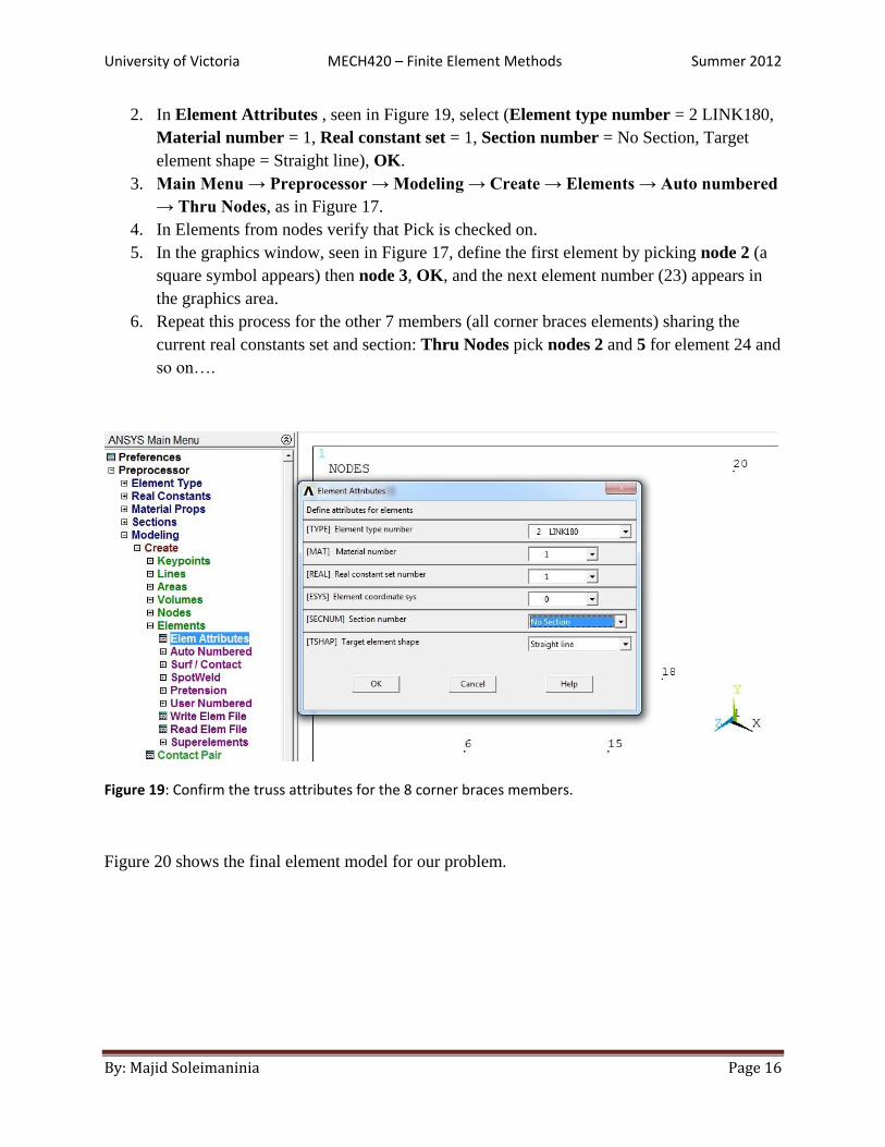
To make corner braces elements from our defined pipe section element:


Attributes.



2. In Element Attributes , seen in Figure 19, select (Element type number = 2 LINK180,

Material number = 1, Real constant set = 1, Section number = No Section, Target

element shape = Straight line), OK.





square symbol appears) then node 3, OK, and the next element number (23) appears in

the graphics area.

6. Repeat this process for the other 7 members (all corner braces elements) sharing the

current real constants set and section: Thru Nodes pick nodes 2 and 5 for element 24 and

so on….

Figure 19: Confirm the truss attributes for the 8 corner braces members.

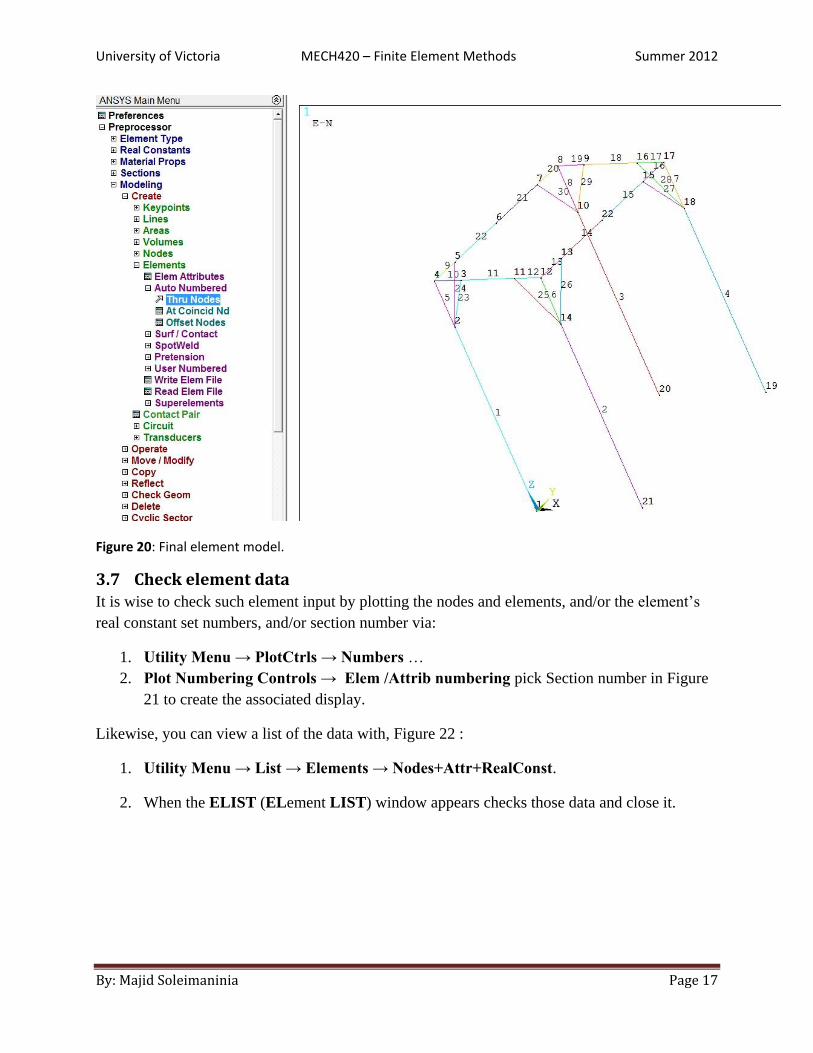
Figure 20 shows the final element model for our problem.



Figure 20: Final element model.

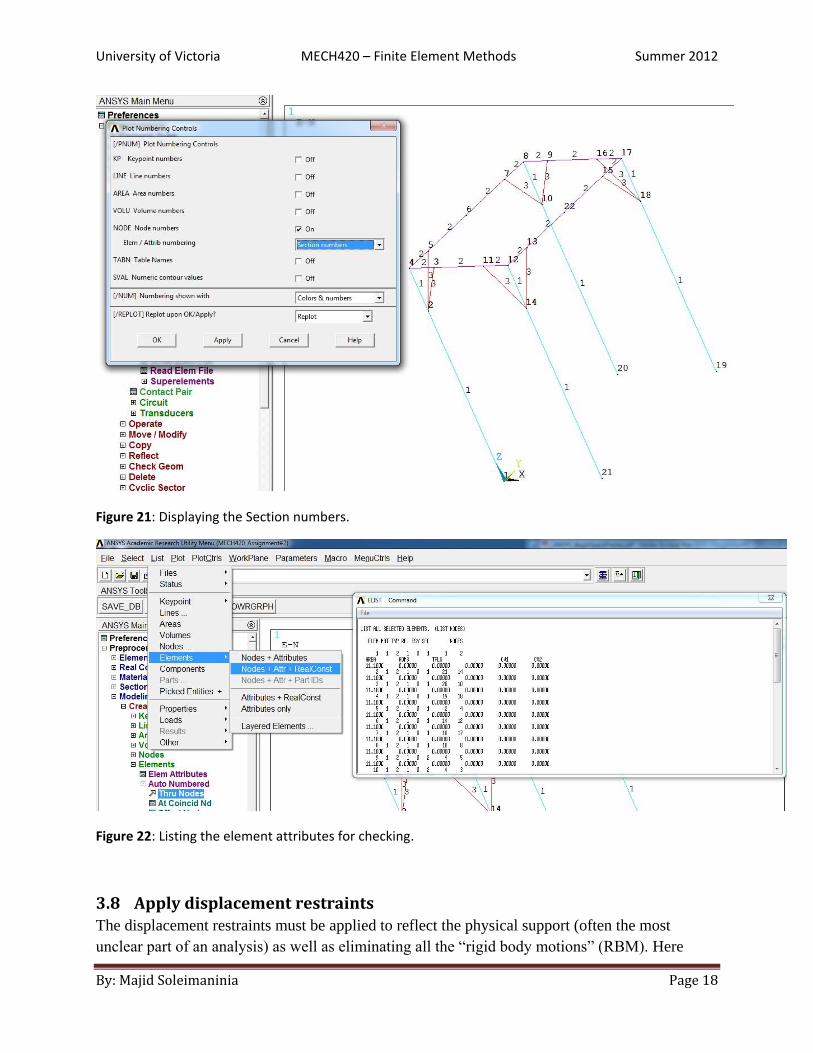
3.7 Check element data It is wise to check such element input by plotting the nodes and elements, and/or the element’s

real constant set numbers, and/or section number via:

1. Utility Menu → PlotCtrls → Numbers …

2. Plot Numbering Controls → Elem /Attrib numbering pick Section number in Figure

21 to create the associated display.

Likewise, you can view a list of the data with, Figure 22 :

1. Utility Menu → List → Elements → Nodes+Attr+RealConst.

2. When the ELIST (ELement LIST) window appears checks those data and close it.



Figure 21: Displaying the Section numbers.

Figure 22: Listing the element attributes for checking.

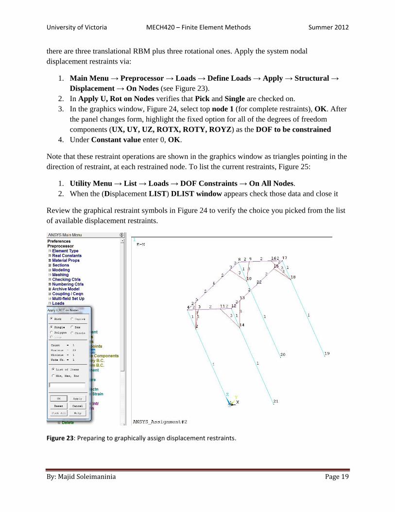
3.8 Apply displacement restraints

The displacement restraints must be applied to reflect the physical support (often the most

unclear part of an analysis) as well as eliminating all the “rigid body motions” (RBM). Here



there are three translational RBM plus three rotational ones. Apply the system nodal

displacement restraints via:

1. Main Menu → Preprocessor → Loads → Define Loads → Apply → Structural →

Displacement → On Nodes (see Figure 23).

2. In Apply U, Rot on Nodes verifies that Pick and Single are checked on.

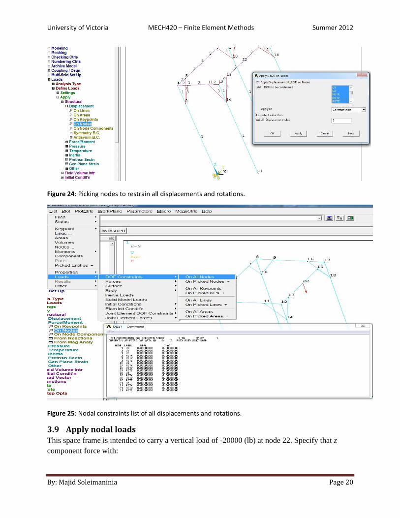
3. In the graphics window, Figure 24, select top node 1 (for complete restraints), OK. After

the panel changes form, highlight the fixed option for all of the degrees of freedom

components (UX, UY, UZ, ROTX, ROTY, ROYZ) as the DOF to be constrained

4. Under Constant value enter 0, OK.

Note that these restraint operations are shown in the graphics window as triangles pointing in the

direction of restraint, at each restrained node. To list the current restraints, Figure 25:

1. Utility Menu → List → Loads → DOF Constraints → On All Nodes.

2. When the (Displacement LIST) DLIST window appears check those data and close it

Review the graphical restraint symbols in Figure 24 to verify the choice you picked from the list

of available displacement restraints.

Figure 23: Preparing to graphically assign displacement restraints.



Figure 24: Picking nodes to restrain all displacements and rotations.

Figure 25: Nodal constraints list of all displacements and rotations.

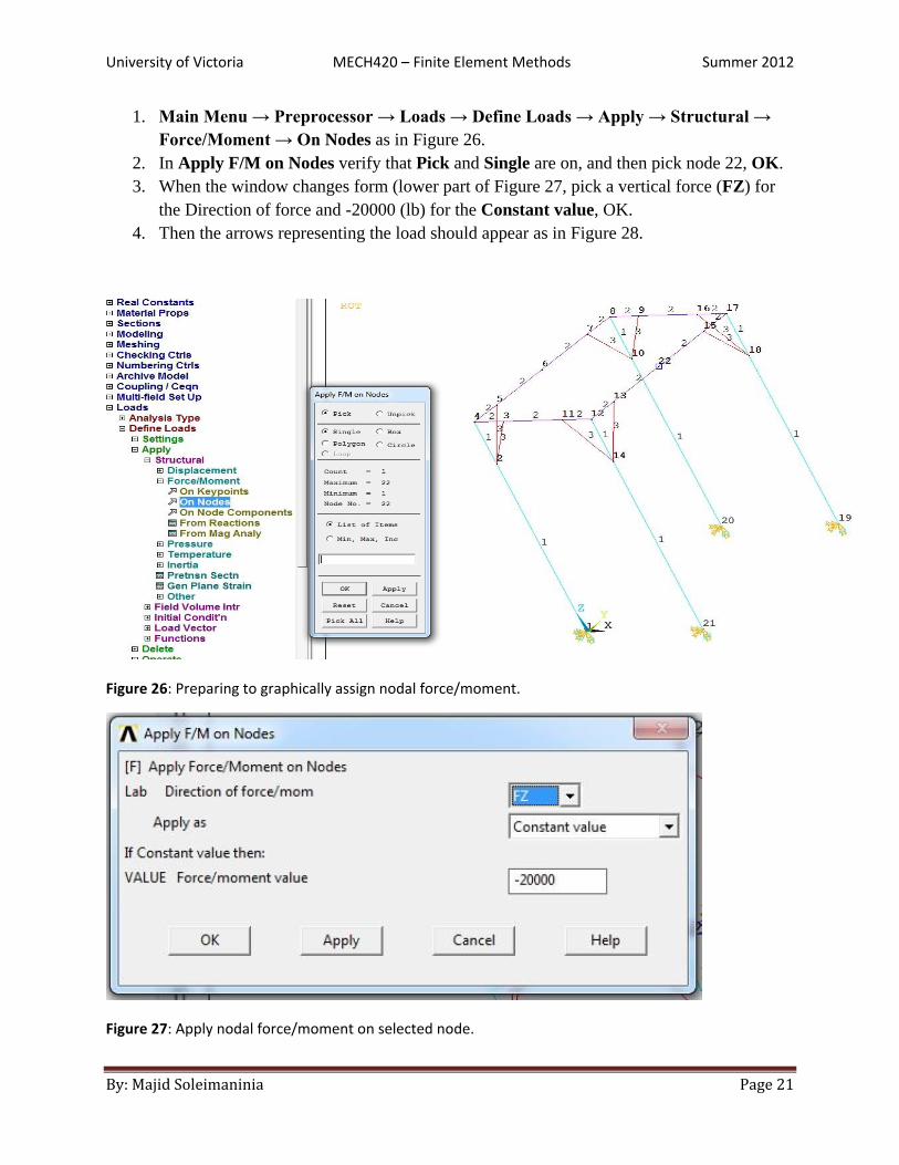
3.9 Apply nodal loads

This space frame is intended to carry a vertical load of -20000 (lb) at node 22. Specify that z

component force with:



1. Main Menu → Preprocessor → Loads → Define Loads → Apply → Structural →

Force/Moment → On Nodes as in Figure 26.

2. In Apply F/M on Nodes verify that Pick and Single are on, and then pick node 22, OK.

3. When the window changes form (lower part of Figure 27, pick a vertical force (FZ) for

the Direction of force and -20000 (lb) for the Constant value, OK.

4. Then the arrows representing the load should appear as in Figure 28.

Figure 26: Preparing to graphically assign nodal force/moment.

Figure 27: Apply nodal force/moment on selected node.



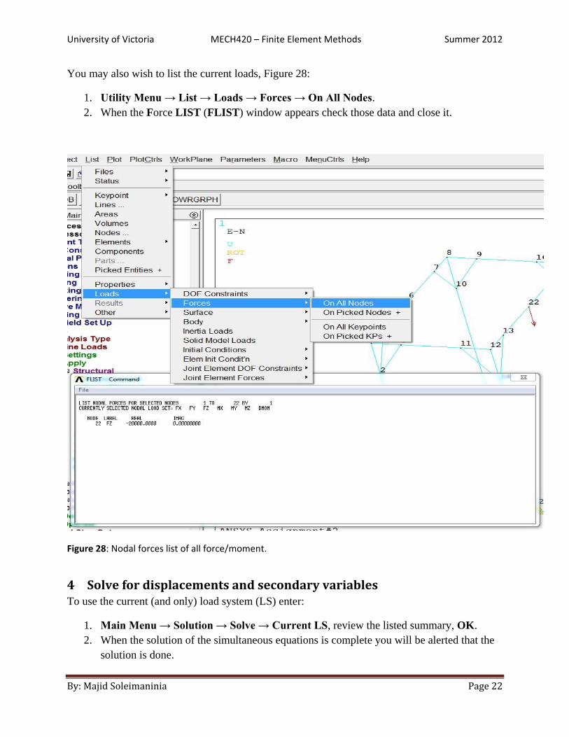
You may also wish to list the current loads, Figure 28:

1. Utility Menu → List → Loads → Forces → On All Nodes.

2. When the Force LIST (FLIST) window appears check those data and close it.

Figure 28: Nodal forces list of all force/moment.

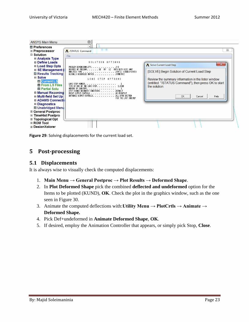
4 Solve for displacements and secondary variables To use the current (and only) load system (LS) enter:

1. Main Menu → Solution → Solve → Current LS, review the listed summary, OK.

2. When the solution of the simultaneous equations is complete you will be alerted that the

solution is done.



Figure 29: Solving displacements for the current load set.

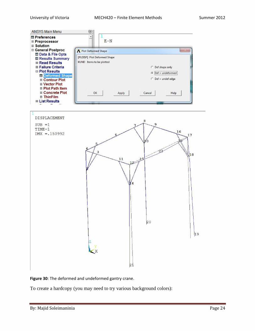
5 Post-processing

5.1 Displacements

It is always wise to visually check the computed displacements:

1. Main Menu → General Postproc → Plot Results → Deformed Shape.

2. In Plot Deformed Shape pick the combined deflected and undeformed option for the

Items to be plotted (KUND), OK. Check the plot in the graphics window, such as the one

seen in Figure 30.

3. Animate the computed deflections with:Utility Menu → PlotCrtls → Animate →

Deformed Shape.

4. Pick Def+undeformed in Animate Deformed Shape, OK.

5. If desired, employ the Animation Controller that appears, or simply pick Stop, Close.



Figure 30: The deformed and undeformed gantry crane.

To create a hardcopy (you may need to try various background colors):



1. Utility Menu → PlotCrtls → Hard Copy → Printer (or → File), select your printer

name, Print.

2. To get the reverse video white background of Figure 30 use PlotCtrls → Style → Color

→ Reverse Video.

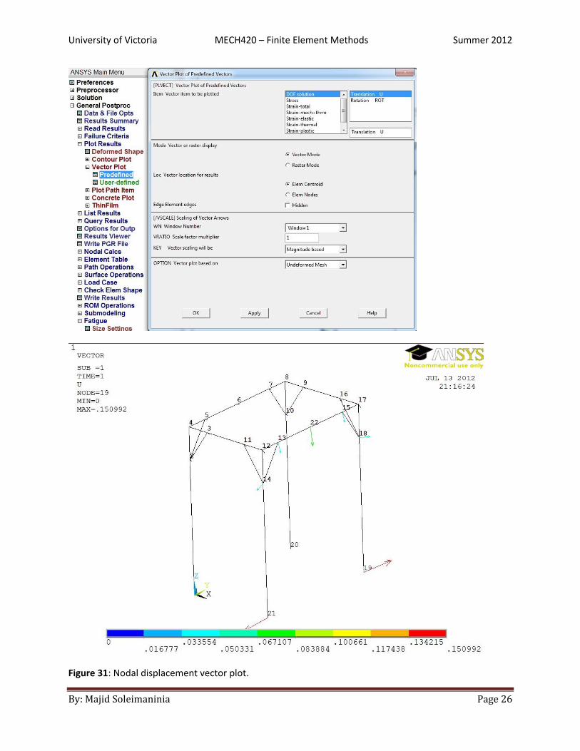
Since displacements and (infinitesimal) rotations are vector quantities it is wise to plot them in

that mode as a visual check of the response of the system. To do that:

1. General Postproc → Plot Results → Vector Plot → Predefined.

2. In Vector Plot of Predefined Vectors select DOF solution, Translation U, Vector

mode, and element nodes.

The resulting color plot will display the vectors with scaled lengths and with a color matching

the color bar scale, as seen in Figure 31.

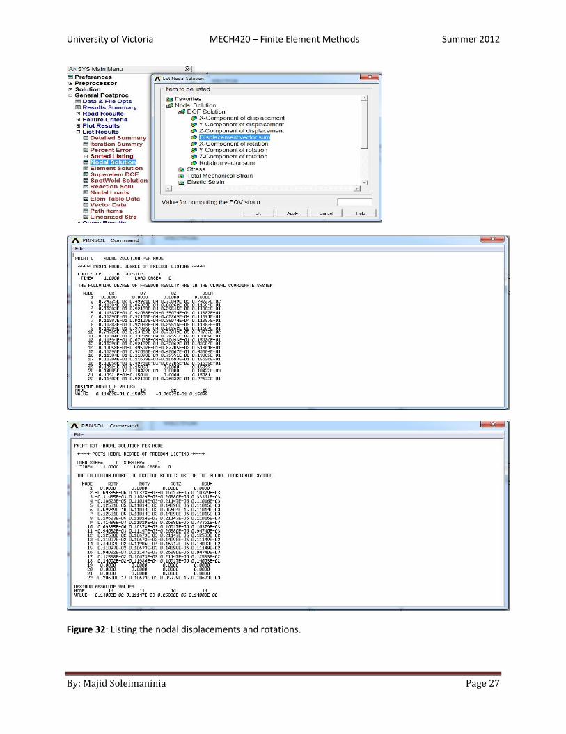
To see a (potentially long) list of displacement results:

1. Preferences → General Postproc → List Results → Nodal Solution.

2. In List Nodal Solution → Nodal Solutions → DOF Solution → Displacement vector

sum, OK.

3. Examine the results in the PRNSOL (PRint Nodal SOLution) Command window of

Figure 26 and close it.

4. Likewise, to see the nodal rotations, also in Figure 26, use List Nodal Solution →

Nodal Solutions → DOF Solution → Rotation vector sum, OK.



Figure 31: Nodal displacement vector plot.



Figure 32: Listing the nodal displacements and rotations.

ansys tutorial for assignment 2

Documents