ant colony system: a cooperative learning approach …lombardy/ens/javattt0708/fourmis.pdf ·...

Dorigo and Gambardella - Ant Colony System 1

Ant Colony System:A Cooperative Learning Approach to the

Traveling Salesman Problem

TR/IRIDIA/1996-5Université Libre de Bruxelles

Belgium

Marco DorigoIRIDIA, Université Libre de Bruxelles, CP 194/6, Avenue Franklin Roosevelt 501050 Bruxelles, [email protected], http://iridia.ulb.ac.be/dorigo/dorigo.html

Luca Maria GambardellaIDSIA, Corso Elvezia 36, 6900 Lugano, [email protected], http://www.idsia.ch/~luca

Abstract

This paper introduces ant colony system (ACS), a distributed algorithm that is appliedto the traveling salesman problem (TSP). In ACS, a set of cooperating agents calledants cooperate to find good solutions to TSPs. Ants cooperate using an indirect form ofcommunication mediated by pheromone they deposit on the edges of the TSP graphwhile building solutions. We study ACS by running experiments to understand itsoperation. The results show that ACS outperforms other nature-inspired algorithmssuch as simulated annealing and evolutionary computation, and we conclude comparingACS-3-opt, a version of ACS augmented with a local search procedure, to some of thebest performing algorithms for symmetric and asymmetric TSPs.

Accepted for publication in the IEEE Transactions on Evolutionary Computation, Vol.1, No.1, 1997. In press.

Dorigo and Gambardella - Ant Colony System 2/24

I. Introduction

The natural metaphor on which ant algorithms are based is that of ant colonies. Real ants arecapable of finding the shortest path from a food source to their nest [3], [22] without usingvisual cues [24] by exploiting pheromone information. While walking, ants depositpheromone on the ground, and follow, in probability, pheromone previously deposited byother ants. A way ants exploit pheromone to find a shortest path between two points is shownin Fig. 1.

Consider Fig. 1A: Ants arrive at a decision point in which they have to decide whether toturn left or right. Since they have no clue about which is the best choice, they chooserandomly. It can be expected that, on average, half of the ants decide to turn left and the otherhalf to turn right. This happens both to ants moving from left to right (those whose namebegins with an L) and to those moving from right to left (name begins with a R). Figs. 1Band 1C show what happens in the immediately following instants, supposing all ants walk atapproximately the same speed. The number of dashed lines is roughly proportional to theamount of pheromone that the ants have deposited on the ground. Since the lower path isshorter than the upper one, more ants will visit it on average, and therefore pheromoneaccumulates faster. After a short transitory period the difference in the amount of pheromoneon the two path is sufficiently large so as to influence the decision of new ants coming intothe system (this is shown by Fig. 1D). From now on, new ants will prefer in probability tochoose the lower path, since at the decision point they perceive a greater amount ofpheromone on the lower path. This in turn increases, with a positive feedback effect, thenumber of ants choosing the lower, and shorter, path. Very soon all ants will be using theshorter path.

R2R1L1L2

? ?R2

R1

L1

L2

R4R3L3L4

R2

R1

L1

R4L5L6 R6R5

L3

L4

L2

R3

R2

R1

L1

R4

R3

L6L7 R7R6

L3

L4

L2

L5 R5

A B

C D

Fig. 1. How real ants find a shortest path. A) Ants arrive at a decision point. B) Some ants choose the upperpath and some the lower path. The choice is random. C) Since ants move at approximately constant speed, theants which choose the lower, shorter, path reach the opposite decision point faster than those which choose theupper, longer, path. D) Pheromone accumulates at a higher rate on the shorter path. The number of dashed linesis approximately proportional to the amount of pheromone deposited by ants.


The above behavior of real ants has inspired ant system , an algorithm in which a set ofartificial ants cooperate to the solution of a problem by exchanging information viapheromone deposited on graph edges. Ant system has been applied to combinatorialoptimization problems such as the traveling salesman problem (TSP) [7], [8], [10], [12], andthe quadratic assignment problem [32], [42].

Ant colony system (ACS), the algorithm presented in this article, builds on the previous antsystem in the direction of improving efficiency when applied to symmetric and asymmetricTSPs. The main idea is that of having a set of agents, called ants, search in parallel for goodsolutions to the TSP, and cooperate through pheromone-mediated indirect and globalcommunication. Informally, each ant constructs a TSP solution in an iterative way: it addsnew cities to a partial solution by exploiting both information gained from past experienceand a greedy heuristic. Memory takes the form of pheromone deposited by ants on TSPedges, while heuristic information is simply given by the edge's length.

The main novel idea introduced by ant algorithms, which will be discussed in theremainder of the paper, is the synergistic use of cooperation among many relatively simpleagents which communicate by distributed memory implemented as pheromone deposited onedges of a graph.

The article is organized as follows. Section II puts ACS in context by describing antsystem, the progenitor of ACS. Section III introduces ACS. Section IV is dedicated to thestudy of some characteristics of ACS: We study how pheromone changes at run time,estimate the optimal number of ants to be used, observe the effects of pheromone-mediatedcooperation, and evaluate the role that pheromone and the greedy heuristic have in ACSperformance. Section V provides an overview of results on a set of standard test problemsand comparisons of ACS with well-known general purpose algorithms like evolutionarycomputation and simulated annealing. In Section VI we add local optimization to ACS,obtaining a new algorithm called ACS-3-opt. This algorithm is compared favorably with thewinner of the First International Contest on Evolutionary Optimization [5] on asymmetricTSP (ATSP) problems (see Fig. 2), while it yields a slightly worse performance on TSPproblems. Section VII is dedicated to the discussion of the main characteristics of ACS andindicates directions for further research.

II. Background

Ant system [10] is the progenitor of all our research efforts with ant algorithms, and was firstapplied to the traveling salesman problem (TSP), which is defined in Fig. 2.

Ant system utilizes a graph representation which is the same as that defined in Fig. 2,augmented as follows: in addition to the cost measure δ(r,s), each edge (r,s) has also adesirability measure τ (r,s), called pheromone , which is updated at run time by artificial ants(ants for short). When ant system is applied to symmetric instances of the TSP, τ(r,s)=τ(s,r),but when it is applied to asymmetric instances it is possible that τ(r,s)≠τ(s,r).

Informally, ant system works as follows. Each ant generates a complete tour by choosingthe cities according to a probabilistic state transition rule : Ants prefer to move to cities whichare connected by short edges with a high amount of pheromone. Once all ants havecompleted their tours a global pheromone updating rule (global updating rule, for short) isapplied: A fraction of the pheromone evaporates on all edges (edges that are not refreshedbecome less desirable), and then each ant deposits an amount of pheromone on edges whichbelong to its tour in proportion to how short its tour was (in other words, edges which belong


to many short tours are the edges which receive the greater amount of pheromone). Theprocess is then iterated.

TSP

Let V = {a, ... , z} be a set of cities, A = {(r,s) : r,s ∈ V} be theedge set, and δ(r,s)= δ(s,r) be a cost measure associated with edge(r,s) ∈ A.

The TSP is the problem of finding a minimal cost closed tour that

visits each city once.

In the case cities r ∈ V are given by their coordinates (xr, yr) and δ(r,s) is the Euclidean distance between r and s, then we have an Euclidean TSP.

ATSP

If δ(r,s) ≠ δ(s,r) for at least one edge (r,s) then the TSP becomes anasymmetric TSP (ATSP).

Fig. 2. The traveling salesman problem.

The state transition rule used by ant system, called a random-proportional rule, is given byEq. (1), which gives the probability with which ant k in city r chooses to move to the city s.

p r s

r s r s

r u r us J r

k u J r

k

k

( , ) =

( , ) ( , )

( , ) ( , ) if ( )

otherwise

( )

τ ητ η

β

β[ ] ⋅[ ]

[ ] ⋅[ ]∈

∈∑

0

(1)

where τ is the pheromone, η=1/δ is the inverse of the distance δ(r,s), Jk(r) is the set of citiesthat remain to be visited by ant k positioned on city r (to make the solution feasible), and β isa parameter which determines the relative importance of pheromone versus distance (β>0).

In Eq. (1) we multiply the pheromone on edge (r ,s) by the corresponding heuristic valueη(r,s) . In this way we favor the choice of edges which are shorter and which have a greateramount of pheromone.

In ant system, the global updating rule is implemented as follows. Once all ants have builttheir tours, pheromone is updated on all edges according to

τ α τ τr s r s r skk

m

, , ,( ) ← −( ) ⋅ ( ) + ( )=

∑11

∆ (2)

where ∆τ k

kr s

L r s

,

( ) =( ) ∈

1 if tour done by ant

0 otherwise

, k

,

0<α<1 is a pheromone decay parameter, Lk is the length of the tour performed by ant k, and mis the number of ants.

Pheromone updating is intended to allocate a greater amount of pheromone to shortertours. In a sense, this is similar to a reinforcement learning scheme [2], [26] in which bettersolutions get a higher reinforcement (as happens, for example, in genetic algorithms underproportional selection). The pheromone updating formula was meant to simulate the changein the amount of pheromone due to both the addition of new pheromone deposited by ants on


the visited edges, and to pheromone evaporation.Pheromone placed on the edges plays the role of a distributed long term memory: This

memory is not stored locally within the individual ants, but is distributed on the edges of thegraph. This allows an indirect form of communication called stigmergy [23], [9]. Theinterested reader will find a full description of ant system, of its biological motivations, andcomputational results in [12].

Although ant system was useful for discovering good or optimal solutions for small TSPs(up to 30 cities), the time required to find such results made it unfeasible for larger problems.We devised three main changes to improve its performance which led to the definition ofACS, presented in the next section.

III. ACS

ACS differs from the previous ant system because of three main aspects: (i) the statetransition rule provides a direct way to balance between exploration of new edges andexploitation of a priori and accumulated knowledge about the problem, (ii) the globalupdating rule is applied only to edges which belong to the best ant tour, and (iii) while antsconstruct a solution a local pheromone updating rule (local updating rule, for short) isapplied.

Informally, ACS works as follows: m ants are initially positioned on n cities chosenaccording to some initialization rule (e.g., randomly). Each ant builds a tour (i.e., a feasiblesolution to the TSP) by repeatedly applying a stochastic greedy rule (the state transition rule).While constructing its tour, an ant also modifies the amount of pheromone on the visitededges by applying the local updating rule. Once all ants have terminated their tour, theamount of pheromone on edges is modified again (by applying the global updating rule). Aswas the case in ant system, ants are guided, in building their tours, by both heuristicinformation (they prefer to choose short edges), and by pheromone information: An edgewith a high amount of pheromone is a very desirable choice. The pheromone updating rulesare designed so that they tend to give more pheromone to edges which should be visited byants. The ACS algorithm is reported in Fig. 3. In the following we discuss the state transitionrule, the global updating rule, and the local updating rule.

A. ACS state transition rule

In ACS the state transition rule is as follows: an ant positioned on node r chooses the city s tomove to by applying the rule given by Eq. (3)

s

r u r u q qu J rk

=

if (exploitation)

otherwise (biased exploration)

arg max , ,∈ ( )

( )[ ] ⋅ ( )[ ]{ } ≤

τ η β0

S(3)

where q is a random number uniformly distributed in [0 .. 1], q0 is a parameter (0≤q0≤1), andS is a random variable selected according to the probability distribution given in Eq. (1).

The state transition rule resulting from Eqs. (3) and (1) is called pseudo-random-proportional rule. This state transition rule, as with the previous random-proportional rule,favors transitions towards nodes connected by short edges and with a large amount ofpheromone. The parameter q0 determines the relative importance of exploitation versusexploration: Every time an ant in city r has to choose a city s to move to, it samples a random


number 0≤q≤1. If q≤q0 then the best edge (according to Eq. (3)) is chosen (exploitation),otherwise an edge is chosen according to Eq. (1) (biased exploration).

Initialize

Loop /* at this level each loop is called an iteration */

Each ant is positioned on a starting node

Loop /* at this level each loop is called a step */Each ant applies a state transition rule to incrementally build a solutionand a local pheromone updating rule

Until all ants have built a complete solution

A global pheromone updating rule is applied

Until End_condition

Fig. 3. The ACS algorithm.

B. ACS global updating rule

In ACS only the globally best ant (i.e., the ant which constructed the shortest tour from thebeginning of the trial) is allowed to deposit pheromone. This choice, together with the use ofthe pseudo-random-proportional rule, is intended to make the search more directed: Antssearch in a neighborhood of the best tour found up to the current iteration of the algorithm.Global updating is performed after all ants have completed their tours. The pheromone levelis updated by applying the global updating rule of Eq. (4)

τ α τ α τr s r s r s, , ,( ) ← −( ) ⋅ ( ) + ⋅ ( )1 ∆ (4)

where ∆τ r sL r sgb

,

-1

( ) =( ) ( ) ∈

if global - best - tour

0 otherwise

,,

0<α<1 is the pheromone decay parameter, and Lgb is the length of the globally best tour fromthe beginning of the trial. As was the case in ant system, global updating is intended toprovide a greater amount of pheromone to shorter tours. Eq. (4) dictates that only those edgesbelonging to the globally best tour will receive reinforcement. We also tested another typeof global updating rule, called iteration-best, as opposed to the above called global-best ,which instead used Lib (the length of the best tour in the current iteration of the trial), in Eq.(4). Also, with iteration-best the edges which receive reinforcement are those belonging tothe best tour of the current iteration. Experiments have shown that the difference between thetwo schemes is minimal, with a slight preference for global-best, which is therefore used inthe following experiments.

C. ACS local updating rule

While building a solution (i.e., a tour) of the TSP, ants visit edges and change theirpheromone level by applying the local updating rule of Eq. (5)

τ ρ τ ρ τr s r s r s, , ,( ) ← −( ) ⋅ ( ) + ⋅ ( )1 ∆ (5)

where 0<ρ<1 is a parameter.

We have experimented with three values for the term ∆τ(r,s). The first choice was looselyinspired by Q-learning [40], an algorithm developed to solve reinforcement learning problems


[26]. Such problems are faced by an agent that must learn the best action to perform in eachpossible state in which it finds itself, using as the sole learning information a scalar numberwhich represents an evaluation of the state entered after it has performed the chosen action.Q-learning is an algorithm which allows an agent to learn such an optimal policy by therecursive application of a rule similar to that in Eq. (5), in which the term ∆τ(r,s) is set to thediscounted evaluation of the next state value. Since the problem our ants have to solve issimilar to a reinforcement learning problem (ants have to learn which city to move to as afunction of their current location), we set [19] ∆τ γ τr s s z

z J sk

, ,( ) = ⋅ ( )∈ ( )max , which is exactly the

same formula used in Q-learning (0≤γ<1 is a parameter). The other two choices were: (i) we

set ∆τ (r,s)=τ0 , whereτ0 is the initial pheromone level, (ii) we set ∆τ(r,s)=0. Finally, we alsoran experiments in which local-updating was not applied (i.e., the local updating rule is notused, as was the case in ant system).

Results obtained running experiments (see Table I) on a set of five randomly generated 50-city TSPs [13], on the Oliver30 symmetric TSP [41], and the ry48p asymmetric TSP [35]essentially suggest that local-updating is definitely useful, and that the local updating rulewith ∆τ (r,s)=0 yields worse performance than local-updating with ∆ τ(r,s)=τ0 or with∆τ γ τr s s z

z J sk

, ,( ) = ⋅ ( )∈ ( )max .

ACS with ∆τ γ τr s s zz J sk

, ,( ) = ⋅ ( )∈ ( )max , which we have called Ant-Q in [11] and [19], and

ACS with ∆τ (r,s)=τ0, called simply ACS hereafter, resulted to be the two best performingalgorithms, with a similar performance level. Since the ACS local updating rule requires lesscomputation than Ant-Q, we chose to focus attention on ACS, which will be used to run theexperiments presented in the following of this paper.

As will be discussed in Section IV.A, the role of ACS local updating rule is to shuffle thetours, so that the early cities in one ant’s tour may be explored later in other ants’ tours. Inother words, the effect of local-updating is to make the desirability of edges changedynamically: every time an ant uses an edge this becomes slightly less desirable (since itloses some of its pheromone). In this way ants will make a better use of pheromoneinformation: without local-updating all ants would search in a narrow neighborhood of thebest previous tour.

D. ACS parameter settings

In all experiments of the following sections the numeric parameters, except when indicateddifferently, are set to the following values: β=2, q0=0.9, α=ρ=0.1, τ0=(n·Lnn)-1 , where Lnn isthe tour length produced by the nearest neighbor heuristic1 [36] and n is the number of cities.These values were obtained by a preliminary optimization phase, in which we found that theexperimental optimal values of the parameters were largely independent of the problem,except for τ0 for which, as we said, τ0 =(n·Lnn)-1 . The number of ants used is m =10 (thischoice is explained in Section IV.B). Regarding their initial positioning, ants are placedrandomly, with at most one ant in each city.

1 To be true, any very rough approximation of the optimal tour length would suffice.


TABLE I

A comparison of local updating rules. 50-city problems and Oliver30 were stopped after 2,500 iterations, whilery48p was halted after 10,000 iterations. Averages are over 25 trials. Results in bold are the best in the Table.

ACS Ant-Q ACS with ∆τ(r,s)=0ACS without

local-updating

average stddev

best average stddev

best average stddev

best average stddev

best

City Set 1 5.88 0.05 5.84 5.88 0.05 5.84 5.97 0.09 5.85 5.96 0.09 5.84

City Set 2 6.05 0.03 5.99 6.07 0.07 5.99 6.13 0.08 6.05 6.15 0.09 6.05

City Set 3 5.58 0.01 5.57 5.59 0.05 5.57 5.72 0.12 5.57 5.68 0.14 5.57

City Set 4 5.74 0.03 5.70 5.75 0.04 5.70 5.83 0.12 5.70 5.79 0.05 5.71

City Set 5 6.18 0.01 6.17 6.18 0.01 6.17 6.29 0.11 6.17 6.27 0.09 6.17

Oliver30 424.74 2.83 423.74 424.70 2.00 423.74 427.52 5.21 423.74 427.31 3.63 423.91

ry48p 14,625 142 14,422 14,766 240 14,422 15,196 233 14,734 15,308 241 14,796

IV. A study of some characteristics of ACS

A. Pheromone behavior and its relation to performance

To try to understand which mechanism ACS uses to direct the search we study how thepheromone–closeness product τ(r,s)[ ] ⋅ η(r,s)[ ]β changes at run time. Fig. 4 shows how thepheromone–closeness product changes with the number of steps while ants are building asolution2 (steps refer to the inner loop in Fig. 3: the abscissa goes therefore from 1 to n,where n is the number of cities).

Let us consider three families of edges (see Fig. 4): (i) those belonging to the last best tour(BE, Best Edges), (ii) those which do not belong to the last best tour, but which did in one ofthe two preceding iterations (TE, Testable Edges), (iii) the remaining edges, that is, those thathave never belonged to a best tour or have not in the last two iterations (UE, UninterestingEdges). The average pheromone–closeness product is then computed as the average ofpheromone–closeness values of all the edges within a family. The graph clearly shows thatACS favors exploitation of edges in BE (BE edges are chosen with probability q0=0.9) andexploration of edges in TE (recall that, since Eqs. (3) and (1), edges with higher pheromone–closeness product have a higher probability of being explored).

An interesting aspect is that while edges are visited by ants, the application of the localupdating rule, Eq. (5), makes their pheromone diminish, making them less and less attractive,and therefore favoring the exploration of edges not yet visited. Local updating has the effectof lowering the pheromone on visited edges so that these become less desirable and thereforewill be chosen with a lower probability by the other ants in the remaining steps of an iterationof the algorithm. As a consequence, ants never converge to a common path. This fact, whichwas observed experimentally, is a desirable property given that if ants explore different pathsthen there is a higher probability that one of them will find an improving solution than there isin the case that they all converge to the same tour (which would make the use of m antspointless).

Experimental observation has shown that edges in BE, when ACS achieves a goodperformance, will be approximately downgraded to TE after an iteration of the algorithm (i.e.,one external loop in Fig. 3; see also Fig. 4), and that edges in TE will soon be downgraded toUE, unless they happen to belong to a new shortest tour.

2 Graph in Fig. 4 is an abstraction of graphs obtained experimentally. Examples of these are given in Fig. 5.


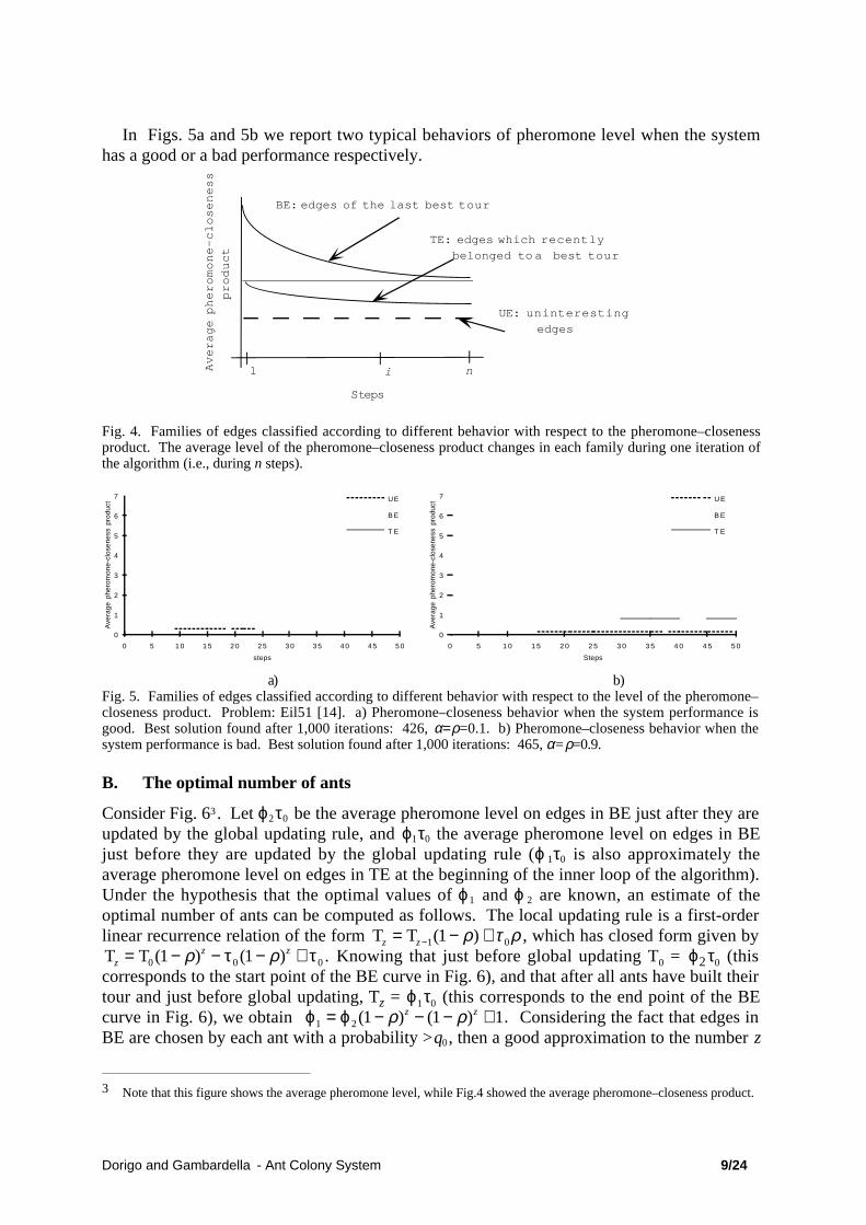
In Figs. 5a and 5b we report two typical behaviors of pheromone level when the systemhas a good or a bad performance respectively.

ni1

BE: edges of the last best tour

TE: edges which recently

belonged to a best tour

UE: uninteresting

edges

Steps

Average pheromone—closeness

product

Fig. 4. Families of edges classified according to different behavior with respect to the pheromone–closenessproduct. The average level of the pheromone–closeness product changes in each family during one iteration ofthe algorithm (i.e., during n steps).

steps

Ave

rage

phe

rom

one-

clos

enes

s pr

oduc

t

0

1

2

3

4

5

6

7

0 5 1 0 1 5 2 0 2 5 3 0 3 5 4 0 4 5 5 0

U E

B E

T E

Steps

Ave

rage

phe

rom

one-

clos

enes

s pr

oduc

t

0

1

2

3

4

5

6

7

0 5 1 0 1 5 2 0 2 5 3 0 3 5 4 0 4 5 5 0

U E

B E

T E

a) b)Fig. 5. Families of edges classified according to different behavior with respect to the level of the pheromone–closeness product. Problem: Eil51 [14]. a) Pheromone–closeness behavior when the system performance isgood. Best solution found after 1,000 iterations: 426, α=ρ=0.1. b) Pheromone–closeness behavior when thesystem performance is bad. Best solution found after 1,000 iterations: 465, α=ρ=0.9.

B. The optimal number of ants

Consider Fig. 63. Let ϕ2τ0 be the average pheromone level on edges in BE just after they areupdated by the global updating rule, and ϕ1τ0 the average pheromone level on edges in BEjust before they are updated by the global updating rule (ϕ 1τ0 is also approximately theaverage pheromone level on edges in TE at the beginning of the inner loop of the algorithm).Under the hypothesis that the optimal values of ϕ1 and ϕ 2 are known, an estimate of theoptimal number of ants can be computed as follows. The local updating rule is a first-orderlinear recurrence relation of the form T Tz z= − +−1 01( )ρ τ ρ , which has closed form given byT Tz

z z= − − − +0 0 01 1( ) ( )ρ ρτ τ . Knowing that just before global updating T0 = ϕ2τ0 (thiscorresponds to the start point of the BE curve in Fig. 6), and that after all ants have built theirtour and just before global updating, Tz = ϕ1τ0 (this corresponds to the end point of the BEcurve in Fig. 6), we obtain ϕ ϕ1 2 1 1 1= − − − +( ) ( )ρ ρz z . Considering the fact that edges inBE are chosen by each ant with a probability >q0, then a good approximation to the number z

3 Note that this figure shows the average pheromone level, while Fig.4 showed the average pheromone–closeness product.


of ants that locally update edges in BE is given by z=m·q0. Substituting in the above formulawe obtain the following estimate of the optimal number of ants

m =log(ϕ

1− 1) − log(ϕ

2− 1)

q0

⋅ log(1 − ρ)

This formula essentially shows that the optimal number of ants is a function of ϕ1 and ϕ 2.Unfortunately, up to now, we have not been able to identify the form of the functions ϕ1(n)and ϕ 2(n), which would tell how ϕ1 and ϕ2 change as a function of the problem dimension .Still, experimental observation shows that ACS works well when the ratio (ϕ1-1)/(ϕ 2-1)≈0.4,which gives m =10.

τ0

ϕ2τ0

ϕ1τ0

ni1

BE: edges of the last best tour

UE: uninteresting

edges

Steps

Average pheromone level

Fig. 6. Change in average pheromone level during an algorithm iteration for edges in the BE family. Theaverage pheromone level on edges in BE starts at ϕ2τ0 and decreases each time an ant visits an edge in BE.After one algorithm iteration, each edge in BE has been visited on average m ·q0 times, and the final value of thepheromone level is ϕ1τ0.

C. Cooperation among ants

This section presents the results of two simple experiments which show that ACS effectivelyexploits pheromone-mediated cooperation. Since artificial ants cooperate by exchanginginformation via pheromone, to have noncooperating ants it is enough to make ants blind topheromone. In practice this is obtained by deactivating Eqs. (4) and (5), and setting the initiallevel of pheromone to τ0=1 on all edges. When comparing a colony of cooperating ants witha colony of noncooperating ants, to make the comparison fair, we use CPU time to computeperformance indexes so as to discount for the higher complexity, due to pheromone updating,of the cooperative approach.

In the first experiment, the distribution of first finishing times , defined as the time elapseduntil the first optimal solution is found, is used to compare the cooperative and thenoncooperative approaches. The algorithm is run 10,000 times, and then we report on a graphthe probability distribution (density of probability) of the CPU time needed to find the optimalvalue (e.g., if in 100 trials the optimum is found after exactly 220 iterations, then for thevalue 220 of the abscissa we will have P(220) = 100/10,000). Fig. 7 shows that cooperationgreatly improves the probability of finding quickly an optimal solution.

In the second experiment (Fig. 8) the best solution found is plotted as a function of time(ms) for cooperating and noncooperating ants. The number of ants is fixed for both cases:m=4. It is interesting to note that in the cooperative case, after 300 ms, ACS always found theoptimal solution, while noncooperating ants where not able to find it after 800 ms. During the


first 150 ms (i.e., before the two lines in Fig. 8 cross) noncooperating ants outperformcooperating ants: Good values of pheromone level are still being learned and therefore theoverhead due to pheromone updating is not yet compensated by the advantages whichpheromone can provide in terms of directing the search towards good solutions.

CPU time (sec)

Den

sity

of

prob

abili

ty

0

0.01

0.02

0.03

0.04

0.05

0.06

0 1 0 2 0 3 0 4 0 5 0 6 0 7 0 8 0 9 0 100

Cooperating ants

Noncooperatingants

Fig. 7. Cooperation changes the probability distribution of first finishing times: cooperating ants have a higherprobability to find quickly an optimal solution. Test problem: CCAO [21]. The number of ants was set to m=4.

Cpu time (msec)

Tou

r le

ngth

49.5

5 0

50.5

5 1

51.5

5 2

52.5

0 100 200 300 400 500 600 700 800

Cooperating ants

Noncooperatingants

Fig. 8. Cooperating ants find better solutions in a shorter time. Test problem: CCAO [21]. Average on 25 runs.The number of ants was set to m=4.

D. The importance of the pheromone and the heuristic function

Experimental results have shown that the heuristic function η is fundamental in making thealgorithm find good solutions in a reasonable time. In fact, when β=0 ACS performanceworsens significantly (see the ACS no heuristic graph in Fig. 9).

Fig. 9 also shows the behavior of ACS in an experiment in which ants neither sense nordeposit pheromone (ACS no pheromone graph). The result is that not using pheromone alsodeteriorates performance. This is a further confirmation of the results on the role ofcooperation presented in Section IV.C.

The reason ACS without the heuristic function performs better than ACS withoutpheromone is that in the first case, although not helped by heuristic information, ACS is stillguided by reinforcement provided by the global updating rule in the form of pheromone,while in the second case ACS reduces to a stochastic multi-greedy algorithm.


Number of ants

Ave

rage

len

gth

of t

he b

est

tour

420

425

430

435

440

445

450

455

460

1 2 4 6 8 1 0 1 2 1 4 1 6 1 8 2 0 2 2 2 4 2 6 2 8 3 0

ACS standard

ACS no heuristic

ACS no pheromone

Fig. 9. Comparison between ACS standard, ACS with no heuristic (i.e., we set β=0), and ACS in which antsneither sense nor deposit pheromone. Problem: Oliver30. Averaged over 30 trials, 10,000/m iterations per trial.

V. ACS: Some computational results

We report on two sets of experiments. The first set compares ACS with other heuristics. Thechoice of the test problems was dictated by published results found in the literature. Thesecond set tests ACS on some larger problems. Here the comparison is performed only withrespect to the optimal or the best known result. The behavior of ACS is excellent in bothcases.

Most of the test problems can be found in TSPLIB: http://www.iwr.uni-heidelberg.de/iwr/comopt/soft/ TSPLIB95/TSPLIB.html. When they are not available in thislibrary we explicitly cite the reference where they can be found.

Given that during an iteration of the algorithm each ant produces a tour, in the reportedresults the total number of tours generated is given by the number of iterations multiplied bythe number of ants. The result of each trial is given by the best tour generated by the ants.Each experiment consists of at least 15 trials.

A. Comparison with other heuristics

To compare ACS with other heuristics we consider two sets of TSP problems. The first setcomprises five randomly generated 50-city problems, while the second set is composed ofthree geometric problems4 of between 50 and 100 cities. It is important to test ACS on bothrandom and geometric instances of the TSP because these two classes of problems havestructural differences that can make them difficult for a particular algorithm and at the sametime easy for another one.

Table II reports the results on the random instances. The heuristics with which wecompare ACS are simulated annealing (SA), elastic net (EN), and self organizing map(SOM). Results on SA, EN, and SOM are from [13], [34]. ACS was run for 2,500 iterationsusing 10 ants (this amounts to approximately the same number of tour searched by theheuristics with which we compare our results). ACS results are averaged over 25 trials. Thebest average tour length for each problem is in boldface: ACS almost always offers the bestperformance.

4 Geometric problems are problems taken from the real world (for example, they are generated choosing real cities and realdistances).


TABLE II

Comparison of ACS with other heuristics on random instances of the symmetric TSP. Comparisons on averagetour length obtained on five 50-city problems.

Problem name ACS(average)

SA(average)

EN(average)

SOM(average)

City set 1 5 . 8 8 5 . 8 8 5.98 6.06

City set 2 6.05 6 . 0 1 6.03 6.25

City set 3 5 . 5 8 5.65 5.70 5.83

City set 4 5 . 7 4 5.81 5.86 5.87

City set 5 6 . 1 8 6.33 6.49 6.70

Table III reports the results on the geometric instances. The heuristics with which wecompare ACS in this case are a genetic algorithm (GA), evolutionary programming (EP), andsimulated annealing (SA). ACS is run for 1,250 iterations using 20 ants (this amounts toapproximately the same number of tours searched by the heuristics with which we compareour results). ACS results are averaged over 15 trials. In this case comparison is performed onthe best results, as opposed to average results as in previous Table II (this choice was dictatedby the availability of published results). The difference between integer and real tour lengthis that in the first case distances between cities are measured by integer numbers, while in thesecond case by floating point approximations of real numbers.

TABLE III

Comparison of ACS with other heuristics on geometric instances of the symmetric TSP. We report the bestinteger tour length, the best real tour length (in parentheses) and the number of tours required to find the bestinteger tour length (in square brackets). N/A means “not available.” In the last column the optimal length isavailable only for integer tour lengths.

Problem name ACS GA EP SA Optimum

Eil50

(50-city problem)

425

(427.96)

[1,830]

428

(N/A)

[25,000]

426

(427.86)

[100,000]

443

(N/A)

[68,512]

425

(N/A)

Eil75

(75-city problem)

535

(542.37)

[3,480]

545

(N/A)

[80,000]

542

(549.18)

[325,000]

580

(N/A)

[173,250]

535

(N/A)

KroA100

(100-city problem)

21,282

(21,285.44)

[4,820]

21,761

(N/A)

[103,000]

N/A

(N/A)

[N/A]

N/A

(N/A)

[N/A]

21,282

(N/A)

Results using EP are from [15], and those using GA are from [41] for Eil50, and Eil75, andfrom [6] for KroA100. Results using SA are from [29]. Eil50, Eil75 are from [14] and areincluded in TSPLIB with an additional city as Eil51.tsp and Eil76.tsp. KroA100 is also inTSPLIB. The best result for each problem is in boldface. Again, ACS offers the bestperformance in nearly every case. Only for the Eil50 problem does it find a slightly worsesolution using real-valued distance as compared with EP, but ACS only visits 1,830 tours,while EP used 100,000 such evaluations (although it is possible that EP found its best solutionearlier in the run, this is not specified in the paper [15]).


B. ACS on some bigger problems

When trying to solve big TSP problems it is common practice [28], [35] to use a datastructure known as candidate list. A candidate list is a list of preferred cities to be visited; itis a static data structure which contains, for a given city i, the cl closest cities, ordered byincreasing distances; cl is a parameter that we set to c l =15 in our experiments. Weimplemented therefore a version of ACS [20] which incorporates a candidate list: An ant inthis extended version of ACS first chooses the city to move to among those belonging to thecandidate list. Only if none of the cities in the candidate list can be visited then it considersthe rest of the cities. ACS with candidate list (see Table IV) was able to find good results forproblems up to more than 1,500 cities. The time to generate a tour grows only slightly morethan linearly with the number of cities (this is much better than the quadratic growth obtainedwithout the candidate list): On a Sun Sparc–server (50 MHz) it took approximately 0.02 secof CPU time to generate a tour for the d198 problem, 0.05 sec for the pcb442, 0.07 sec for theatt532, 0.13 sec for the rat783, and 0.48 sec for the fl1577 (the reason for the more than linearincrease in time is that the number of failures, that is, the number of times an ant has tochoose the next city outside of the candidate list, increases with the problem dimension).

TABLE IV

ACS performance for some bigger geometric problems (over 15 trials). We report the integer length of theshortest tour found, the number of tours required to find it, the average integer length, the standard deviation , theoptimal solution (for fl1577 we give, in square brackets, the known lower and upper bounds, given that theoptimal solution is not known), and the relative error of ACS.

Problem name ACS

best integerlength

(1)

ACS

number oftours

generatedto best

ACS

averageintegerlength

Standarddeviation

Optimum

(2)

Relative error

(1)-(2) --------- * 100 (2)

d198

(198-city problem)

15,888 585,000 16,054 71 15,780 0.68 %

pcb442

(442-city problem)

51,268 595,000 51,690 188 50,779 0.96 %

att532

(532-city problem)

28,147 830,658 28,523 275 27,686 1.67 %

rat783

(783-city problem)

9,015 991,276 9,066 28 8,806 2.37 %

fl1577

(1577-city problem)

22,977 942,000 23,163 116 [22,204 –22,249]

3.27÷3.48 %


VI. ACS plus local search

In Section V we have shown that ACS is competitive with other nature-inspired algorithmson some relatively simple problems. On the other hand, in the past years a lot of work hasbeen done to define ad-hoc heuristics, see [25] for an overview, to solve the TSP. In general,these ad-hoc heuristics greatly outperform, on the specific problem of the TSP, generalpurpose algorithms approaches like evolutionary computation and simulated annealing.Heuristic approaches to the TSP can be classified as tour constructive heuristics and tourimprovement heuristics (these last also called local optimization heuristics). Tourconstructive heuristics (see [4] for an overview) usually start selecting a random city from theset of cities and then incrementally build a feasible TSP solution by adding new cities chosenaccording to some heuristic rule. For example, the nearest neighbor heuristic builds a tour byadding the closest node in term of distance from the last node inserted in the path. On theother hand, tour improvement heuristics start from a given tour and attempt to reduce itslength by exchanging edges chosen according to some heuristic rule until a local optimum isfound (i.e., until no further improvement is possible using the heuristic rule). The most usedand well-known tour improvement heuristics are 2-opt and 3-opt [30], and Lin-Kernighan[31] in which respectively two, three, and a variable number of edges are exchanged. It hasbeen experimentally shown [35] that, in general, tour improvement heuristics produce betterquality results than tour constructive heuristics. A general approach is to use tourconstructive heuristics to generate a solution and then to apply a tour improvement heuristicto locally optimize it.

It has been shown recently [25] that it is more effective to alternate an improvementheuristic with mutations of the last (or of the best) solution produced, rather than iterativelyexecuting a tour improvement heuristic starting from solutions generated randomly or by aconstructive heuristic. An example of successful application of the above alternate strategy isthe work by Freisleben and Merz [17], [18] in which a genetic algorithm is used to generatenew solutions to be locally optimized by a tour improvement heuristic.

ACS is a tour construction heuristic which, like Freisleben and Merz's genetic algorithm,after each iteration produces a set of feasible solutions which are in some sense a mutation ofthe previous best solution. It is therefore a reasonable guess that adding a tour improvementheuristic to ACS could make it competitive with the best algorithms.

We have therefore added a tour improvement heuristic to ACS. In order to maintain ACSability to solve both TSP and ATSP problems we have decided to base the local optimizationheuristic on a restricted 3-opt procedure [25], [27] that, while inserting/removing three edgeson the path, considers only 3-opt moves that do not revert the order in which the cities arevisited. In this case it is possible to change three edges on the tour (k , l), (p, q) and (r , s) withthree other edges (k, q), (p, s) and (r , l) maintaining the previous orientations of all the othersub-tours. In case of ATSP problems, where in general δ(k, l) ≠ δ(l, k), this 3-opt procedureavoids unpredictable tour length changes due to the inversion of a sub-tour. In addition, whena candidate edge (k, l) to be removed is selected, the rescricted 3-opt procedure restricts thesearch for the second edge (p, q) to be removed only to those edges such that δ(k, q)<δ(k, l).

The implementation of the restricted 3-opt procedure includes some typical tricks whichaccelerate its use for TSP/ATSP problems. First, search for the candidate nodes during therestricted 3-opt procedure is only made inside the candidate list [25]. Second, the procedureuses a data structure called don’t look bit [4] in which each bit is associated to a node of thetour. At the beginning of the local optimization procedure all the bits are turned off and thebit associated to node r is turned on when a search for an improving move starting from r


fails. The bit associated to node r is turned off again when a move involving r is performed.Third, only in the case of symmetric TSPs, while searching for 3-opt moves starting from anode r the procedure also considers possible 2-opt moves with r as first node: the moveexecuted is the best one among those proposed by 3-opt and those proposed by 2-opt. Last, atraditional array data structure to represent candidate lists and tours is used (see [16] for moresophisticated data structures).

Initialize

Loop /* at this level each loop is called an iteration */

Each ant is positioned on a starting node

Loop /* at this level each loop is called a step */Each ant applies a state transition rule to incrementally build a solutionand a local pheromone updating rule

Until all ants have built a complete solution

Each ant is brought to a local minimum using a tour improvement

heuristic based on 3-opt

A global pheromone updating rule is applied

Until End_condition

Fig. 10. The ACS-3-opt algorithm.

ACS-3-opt also uses candidate lists in its constructive part; if there is no feasible node inthe candidate list it chooses the closest node out of the candidate list (this is different fromwhat happens in ACS where, in case the candidate list contains no feasible nodes, then any ofthe remaining feasible cities can be chosen with a probability which is given by thenormalized product of pheromone and closeness). This is a reasonable choice since most ofthe search performed by both ACS and the local optimization procedure is made using edgesbelonging to the candidate lists. It is therefore pointless to direct search by using pheromonelevels which are updated only very rarely.

A. Experimental results

The experiments on ATSP problems presented in this section have been executed on a SUNUltra1 SPARC Station (167Mhz), while experiments on TSP problems on a SGI Challenge Lserver with eight 200 MHz CPU's, using only a single processor due to the sequentialimplementation of ACS-3-opt. For each test problem have been executed 10 trials. ACS-3-opt parameters were set to the following values (except if differently indicated): m=10, β=2,q0=0.98, α=ρ=0.1, τ 0=(n·Lnn)

-1 , cl=20.

A s y m m e t r i c T S P p r o b l e m s

The results obtained with ACS-3-opt on ATSP problems are quite impressive. Experimentswere run on the set of ATSP problems proposed in the First International Contest onEvolutionary Optimization [5], but see also http://iridia.ulb.ac.be/langerman/ICEO.html). Forall the problems ACS-3-opt reached the optimal solution in a few seconds (see Table V) in allthe ten trials, except in the case of ft70, a problem considered relatively hard, where theoptimum was reached 8 out of 10 times.

In Table VI results obtained by ACS-3-opt are compared with those obtained by ATSP-GA[17], the winner of the ATSP competition. ATSP-GA is based on a genetic algorithm thatstarts its search from a population of individuals generated using a nearest neighbor heuristic.


Individuals are strings of cities which represent feasible solutions. At each step two parents xand y are selected and their edges are recombined using a procedure called DPX-ATSP.DPX-ATSP first deletes all edges in x that are not contained in y and then reconnects the seg-ments using a greedy heuristic based on a nearest neighbor choice. The new individuals arebrought to the local optimum using a 3-opt procedure, and a new population is generated afterthe application of a mutation operation that randomly removes and reconnects some edges inthe tour.

TABLE V

Results obtained by ACS-3-opt on ATSP problems taken from the First International Contest on EvolutionaryOptimization [5]. We report the length of the best tour found by ACS-3-opt, the CPU time used to find it, theaverage length of the best tour found and the average CPU time used to find it, the optimal length and therelative error of the average result with respect to the optimal solution.

Problem name ACS-3-opt

best result

(length)

ACS-3-opt

best result

(sec)

ACS-3-opt

average

(length)

ACS-3-opt

average

(sec)

Optimum % Error

p43(43-city problem)

2,810 1 2,810 2 2,810 0.00 %

ry48p

(48-city problem)14,422 2 14,422 19 14,422 0.00 %

ft70

(70-city problem)38,673 3 38,679.8 6 38,673 0.02 %

kro124p

(100-city problem)36,230 3 36,230 25 36,230 0.00 %

ftv170*

(170-city problem)2,755 17 2,755 68 2,755 0.00 %

* ftv170 trials were run setting cl=30.

TABLE VI

Comparison between ACS-3-opt and ATSP-GA on ATSP problems taken from the First International Conteston Evolutionary Optimization [5]. We report the average length of the best tour found, the average CPU timeused to find it, and the relative error with respect to the optimal solution for both approaches.


average

(length)

ACS-3-opt

average

(sec)

ACS-3-opt

% error

ATSP-GA

average

(length)

ATSP-GA

average

(sec)

ATSP-GA

% error

p43

(43-city problem)2,810 2 0.00 % 2,810 10 0.00 %

ry48p

(48-city problem)14,422 19 0.00 % 14,440 30 0.12 %

ft70

(70-city problem)38,679.8 6 0.02 % 38,683.8 639 0.03 %

kro124p

(100-city problem)36,230 25 0.00 % 36,235.3 115 0.01 %

ftv170

(170-city problem)2,755 68 0.00 % 2,766.1 211 0.40 %


The 3-opt procedure used by ATSP-GA is very similar to our restricted 3-opt, whichmakes the comparison between the two approaches straightforward. ACS-3-opt outperformsATSP-GA in terms of both closeness to the optimal solution and of CPU time used.Moreover, ATSP-GA experiments have been performed using a DEC Alpha Station (266MHz), a machine faster than our SUN Ultra1 SPARC Station.

S y m m e t r i c T S P p r o b l e m s

If we now turn to symmetric TSP problems, it turns out that STSP-GA (STSP-GA ex-periments have been performed using a 175 MHz DEC Alpha Station), the algorithm thatwon the First International Contest on Evolutionary Optimization in the symmetric TSPcategory, outperforms ACS-3-opt (see Tables VII and VIII). The results used forcomparisons are those published in [18], which are slightly better than those published in[17].

Our results are, on the other hand, comparable to those obtained by other algorithmsconsidered to be very good. For example, on the lin318 problem ACS-3-opt hasapproximately the same performance as the “large step Markov chain” algorithm [33]. Thisalgorithm is based on a simulated annealing mechanism that uses as improvement heuristic arestricted 3-opt heuristic very similar to ours (the only difference is that they do not consider2-opt moves) and a mutation procedure called double-bridge . (The double-bridge mutationhas the property that it is the smallest change (4 edges) that can not be reverted in one step by3-opt, LK and 2-opt.)

A fair comparison of our results with the results obtained with the currently bestperforming algorithms for symmetric TSPs [25] is difficult since they use as local search aLin-Kernighan heuristic based on a segment-tree data structure [16] that is faster and givesbetter results than our restricted-3-opt procedure. It will be the subject of future work to addsuch a procedure to ACS.

TABLE VII

Results obtained by ACS-3-opt on TSP problems taken from the First International Contest on EvolutionaryOptimization [5]. We report the length of the best tour found by ACS-3-opt, the CPU time used to find it, theaverage length of the best tour found and the average CPU time used to find it, the optimal length and therelative error of the average result with respect to the optimal solution.


best result

(length)

ACS-3-opt

best result

(sec)

ACS-3-opt

average

(length)

ACS-3-opt

average

(sec)

Optimum % Error

d198

(198-city problem)15,780 16 15,781.7 238 15,780 0.01 %

lin318*

(318-city problem)42,029 101 42,029 537 42,029 0.00 %

att532

(532-city problem)27,693 133 27,718.2 810 27,686 0.11 %

rat783

(783-city problem)8,818 1,317 8,837.9 1,280 8,806 0.36 %

* lin318 trials were run setting q0 =0.95.


TABLE VIII

Comparison between ACS-3-opt and STSP-GA on TSP problems taken from the First International Contest onEvolutionary Optimization [5]. We report the average length of the best tour found, the average CPU timeused to find it, and the relative error with respect to the optimal solution for both approaches.


average

(length)

ACS-3-opt

average

(sec)

ACS-3-opt

% error

STSP-GA

average

(length)

STSP-GA

average

(sec)

STSP-GA

% error

d198

(198-city problem)15,781.7 238 0.01 % 15,780 253 0.00 %

lin318

(318-city problem) 42,029 537 0.00 % 42,029 2,054 0.00 %

att532

(532-city problem)27,718.2 810 0.11 % 27,693.7 11,780 0.03 %

rat783

(783-city problem)8,837.9 1,280 0.36 % 8,807.3 21,210 0.01 %

VII. Discussion and conclusions

An intuitive explanation of how ACS works, which emerges from the experimental resultspresented in the preceding sections, is as follows. Once all the ants have generated a tour, thebest ant deposits (at the end of iteration t) its pheromone, defining in this way a “preferredtour” for search in the following algorithm iteration t+1. In fact, during iteration t+1 ants willsee edges belonging to the best tour as highly desirable and will choose them with highprobability. Still, guided exploration (see Eqs. (3) and (1)) together with the fact that localupdating “eats” pheromone away (i.e., it diminishes the amount of pheromone on visitededges, making them less desirable for future ants) allowing for the search of new, possiblybetter tours in the neighborhood5 of the previous best tour. So ACS can be seen as a sort ofguided parallel stochastic search in the neighborhood of the best tour.

Recently there has been growing interest in the application of ant colony algorithms todifficult combinatorial problems. A first example is the work of Schoonderwoerd, Holland,Bruten and Rothkrantz [37] who apply an ant colony algorithm to the load balancing problemin telecommunications networks. Their algorithm takes inspiration from the same biologicalmetaphor as ant system, although their implementation differs in many details due to thedifferent characteristics of the problem. Another interesting ongoing research is that ofStützle and Hoos who are studying various extensions of ant system to improve itsperformance: in [38] they impose an upper and lower bound on the value of pheromone onedges, in [39] they add local search, much in the same spirit as we did in the previous SectionVI.

Besides the two works above, among the "nature-inspired" heuristics, the closest to ACSseems to be Baluja and Caruana’s Population Based Incremental Learning (PBIL) [1]. PBIL,which takes inspiration from genetic algorithms, maintains a vector of real numbers, thegenerating vector, which plays a role similar to that of the population in GAs. Starting fromthis vector, a population of binary strings is randomly generated: Each string in the

5 The form of the neighborhood is given by the previous history of the system, that is, by pheromone accumulated onedges.


population will have the i-th bit set to 1 with a probability which is a function of the i-th valuein the generating vector (in practice, values in the generating vector are normalized to theinterval [0, 1] so that they can directly represent the probabilities). Once a population ofsolutions is created, the generated solutions are evaluated and this evaluation is used toincrease (or decrease) the probabilities in the generating vector so that good (bad) solutions inthe future generations will be produced with higher (lower) probability. When applied toTSP, PBIL uses the following encoding: a solution is a string of size nlog2n bits, where n isthe number of cities; each city is assigned a string of length log2n which is interpreted as aninteger. Cities are then ordered by increasing integer values; in case of ties the leftmost cityin the string comes first in the tour. In ACS, the pheromone matrix plays a role similar toBaluja’s generating vector, and pheromone updating has the same goal as updating theprobabilities in the generating vector. Still, the two approaches are very different since inACS the pheromone matrix changes while ants build their solutions, while in PBIL theprobability vector is modified only after a population of solutions has been generated.Moreover, ACS uses heuristic to direct search, while PBIL does not.

There are a number of ways in which the ant colony approach can be improved and/orchanged. A first possibility regards the number of ants which should contribute to the globalupdating rule. In ant system all the ants deposited their pheromone, while in ACS only thebest one does: obviously there are intermediate possibilities. Baluja and Caruana [1] haveshown that the use of the two best individuals can help PBIL to obtain better results, since theprobability of being trapped in a local minimum becomes smaller. Another change to ACScould be, again taking inspiration from [1], allowing ants which produce very bad tours tosubtract pheromone.

A second possibility is to move from the current parallel local updating of pheromone to asequential one. In ACS all ants apply the local updating rule in parallel, while they arebuilding their tours. We could imagine a modified ACS in which ants build tourssequentially: the first ant starts, builds its tour and, as a side effect, changes the pheromoneon visited edges. Then the second ant starts, and so on until the last of the m ants has built itstour. At this point the global updating rule is applied. This scheme will determine a differentsearch regime, in which the preferred tour will tend to remain the same for all the ants (asopposed to the situation in ACS, in which local updating shuffles the tours). Nevertheless,search will be diversified since the first ants in the sequence will search in a narrowerneighborhood of the preferred tour than later ones (in fact, pheromone on the preferred tourdecreases as more ants eat it away, making the relative desirability of edges of the preferredtour decrease). The role of local updating in this case would be similar to that of thetemperature in simulated annealing, with the main difference that here the temperaturechanges during each algorithm iteration.

Last, it would be interesting to add to ACS a more effective local optimizer than that usedin Section VI. A possibility we will investigate in the near future is the use of the Lin-Kernighan heuristic.

Another interesting subject of ongoing research is to establish the class of problems thatcan be attacked by ACS. Our intuition is that ant colony algorithms can be applied tocombinatorial optimization problems by defining an appropriate graph representation of theproblem considered, and a heuristic that guides the construction of feasible solutions. Then,artificial ants much like those used in the TSP application presented in this paper can be usedto search for good solutions of the problem under consideration. The above intuition issupported by encouraging, although preliminary, results obtained with ant system on the


quadratic assignment problem [12], [32], [42].In conclusion, in this paper we have shown that ACS is an interesting novel approach to

parallel stochastic optimization of the TSP. ACS has been shown to compare favorably withprevious attempts to apply other heuristic algorithms like genetic algorithms, evolutionaryprogramming, and simulated annealing. Nevertheless, competition on the TSP is very tough,and a combination of a constructive method which generates good starting solution with localsearch which takes these solutions to a local optimum seems to be the best strategy [25]. Wehave shown that ACS is also a very good constructive heuristic to provide such startingsolutions for local optimizers.

Appendix A: The ACS algorithm

1./* Initialization phase */For each pair (r,s) τ(r,s):= τ

0 End-forFor k:=1 to m do

Let rk1 be the starting city for ant k

Jk(r

k1):= {1, ..., n} - r

k1/* J

k(r

k1) is the set of yet to be visited cities for

ant k in city rk1 */

rk:= r

k1 /* rk is the city where ant k is located */

End-for2. /* This is the phase in which ants build their tours. The tour of ant k

is stored in Tourk. */

For i:=1 to n do If i<n

Then For k:=1 to m do

Choose the next city sk according to Eq. (3) and Eq. (1)

Jk(s

k):= J

k(r

k) - s

kTour

k(i):=(r

k ,s

k)

End-for Else For k:=1 to m do /* In this cycle all the ants go back to the initial city r

k1 */

sk := rk1Tour

k(i):=(r

k ,s

k)

End-for End-if

/* In this phase local updating occurs and pheromone isupdated using Eq. (5)*/

For k:=1 to m doτ(r

k ,s

k):=(1-ρ)τ(r

k ,s

k)+ ρτ

0rk := s

k /* New city for ant k */ End-for

End-for3. /* In this phase global updating occurs and pheromone is updated */

For k:=1 to m doCompute L

k /* L

k is the length of the tour done by ant k*/

End-forCompute L

best /*Update edges belonging to L

best using Eq. (4) */

For each edge (r,s)τ(r

k ,s

k):=(1-α)τ( r

k ,s

k)+ α (L

best)-1

End-for4. If (End_condition = True)

then Print shortest of Lk

else goto Phase 2


Acknowledgments

Marco Dorigo is a Research Associate with the FNRS. Luca Gambardella is ResearchDirector at IDSIA. This research has been funded by the Swiss National Science Fund,contract 21–45653.95 titled “Cooperation and learning for combinatorial optimization.” Wewish to thank Nick Bradshaw, Gianni Di Caro, David Fogel, and five anonymous referees fortheir precious comments on a previous version of this article.

References[1] S. Baluja and R. Caruana, “Removing the genetics from the standard genetic algorithm,”

Proceedings of ML-95, Twelfth International Conference on Machine Learning, A. Prieditis andS. Russell (Eds.), 1995, Morgan Kaufmann, pp. 38–46.

[2] A.G. Barto, R.S. Sutton, P.S. Brower, “Associative search network: a reinforcement learningassociative memory,” Biological Cybernetics, vol. 40, pp. 201–211, 1981.

[3] R. Beckers, J.L. Deneubourg, and S. Goss, “Trails and U-turns in the selection of the shortestpath by the ant Lasius Niger,” Journal of Theoretical Biology, vol. 159, pp. 397–415, 1992.

[4] J.L. Bentley, “Fast algorithms for geometric traveling salesman problems,” ORSA Journal onComputing , vol. 4, pp. 387–411, 1992.

[5] H. Bersini, M. Dorigo, S. Langerman, G. Seront, and L. M. Gambardella, “Results of the firstinternational contest on evolutionary optimisation (1st ICEO),” Proceedings of IEEEInternational Conference on Evolutionary Computation, IEEE-EC 96, 1996, IEEE Press, pp.611–615.

[6] H. Bersini, C. Oury, and M. Dorigo, “Hybridization of genetic algorithms,” Tech. Rep. No.IRIDIA/95-22, 1995, Université Libre de Bruxelles, Belgium.

[7] A. Colorni, M. Dorigo, and V. Maniezzo, “Distributed optimization by ant colonies,”Proceedings of ECAL91 - European Conference on Artificial Life , Paris, France, 1991, F.Varela and P. Bourgine (Eds.), Elsevier Publishing, pp. 134–142.

[8] A. Colorni, M. Dorigo, and V. Maniezzo, “An investigation of some properties of an antalgorithm,” Proceedings of the Parallel Problem Solving from Nature Conference (PPSN 92),1992, R. Männer and B. Manderick (Eds.), Elsevier Publishing, pp. 509–520.

[9] J.L. Deneubourg, “Application de l’ordre par fluctuations à la description de certaines étapes dela construction du nid chez les termites,” Insect Sociaux , vol. 24, pp. 117–130, 1977.

[10] M. Dorigo, Optimization, learning and natural algorithms. Ph.D.Thesis, DEI, Politecnico diMilano, Italy, 1992. (In Italian.)

[11] M. Dorigo and L.M. Gambardella, “A study of some properties of Ant-Q,” Proceedings ofPPSN IV–Fourth International Conference on Parallel Problem Solving From Nature, H.–M.Voigt, W. Ebeling, I. Rechenberg and H.–S. Schwefel (Eds.), Springer-Verlag, Berlin, 1996, pp.656–665.

[12] M. Dorigo, V. Maniezzo, and A.Colorni, “The ant system: optimization by a colony of coop-erating agents,” IEEE Transactions on Systems, Man, and Cybernetics–Part B, vol. 26, No. 2,pp. 29–41, 1996.

[13] R. Durbin and D. Willshaw, “An analogue approach to the travelling salesman problem usingan elastic net method,” Nature, vol. 326, pp. 689-691, 1987.

[14] S. Eilon, C.D.T. Watson-Gandy, and N. Christofides, “Distribution management: mathematicalmodeling and practical analysis,” Operational Research Quarterly, vol. 20, pp. 37–53, 1969.

[15] D. Fogel, “Applying evolutionary programming to selected traveling salesman problems,”Cybernetics and Systems: An International Journal, vol. 24, pp. 27–36, 1993.

[16] M.L. Fredman, D.S. Johnson, L.A. McGeoch, and G. Ostheimer, “Data structures for travelingsalesmen,” Journal of Algorithms, vol. 18, pp. 432–479, 1995.

[17] B. Freisleben and P. Merz, “Genetic local search algorithm for solving symmetric andasymmetric traveling salesman problems,” Proceedings of IEEE International Conference onEvolutionary Computation, IEEE-EC 96, 1996, IEEE Press, pp. 616-621.


[18] B. Freisleben and P. Merz, “New genetic local search operators for the traveling salesmanproblem,” Proceedings of PPSN IV–Fourth International Conference on Parallel ProblemSolving From Nature, H.–M. Voigt, W. Ebeling, I. Rechenberg and H.–S. Schwefel (Eds.),Springer-Verlag, Berlin, 1996, pp. 890–899.

[19] L. M. Gambardella and M. Dorigo, “Ant-Q: a reinforcement learning approach to the travelingsalesman problem,” Proceedings of ML-95, Twelfth International Conference on MachineLearning, A. Prieditis and S. Russell (Eds.), Morgan Kaufmann, 1995, pp. 252–260.

[20] L.M. Gambardella and M. Dorigo, “Solving symmetric and asymmetric TSPs by ant colonies,”Proceedings of IEEE International Conference on Evolutionary Computation, IEEE-EC 96 ,IEEE Press, 1996, pp. 622–627.

[21] B. Golden and W. Stewart, “Empiric analysis of heuristics,” in The traveling salesman problem,E.L. Lawler, J.K. Lenstra, A.H.G. Rinnooy-Kan, D.B. Shmoys (Eds.), New York: Wiley andSons, 1985.

[22] S. Goss, S. Aron, J.L. Deneubourg, and J.M. Pasteels, “Self-organized shortcuts in the argentineant,” Naturwissenschaften, vol. 76, pp. 579–581, 1989.

[23] P. P. Grassé, “La reconstruction du nid et les coordinations inter-individuelles chezBellicositermes natalensis et Cubitermes sp . La théorie de la stigmergie: Essai d’interprétationdes termites constructeurs,” Insect Sociaux, vol. 6, pp. 41–83, 1959.

[24] B. Hölldobler and E.O. Wilson, The ants . Springer-Verlag, Berlin, 1990.[25] D.S. Johnson and L.A. McGeoch, “The travelling salesman problem: a case study in local

optimization,” in Local Search in Combinatorial Optimization, E.H.L. Aarts and J.K. Lenstra(Eds.), New York: Wiley and Sons, 1997.

[26] L.P. Kaelbling, L.M. Littman and A.W. Moore, “Reinforcement learning: a survey,” Journal ofArtificial Intelligence Research, vol. 4, pp. 237–285, 1996.

[27] P-C. Kanellakis and C.H. Papadimitriou, “Local search for the asymmetric traveling salesmanproblem,” Operations Research, vol. 28, no. 5, pp. 1087–1099, 1980.

[28] E. L. Lawler, J. K. Lenstra, A. H. G. Rinnooy-Kan, and D. B. Shmoys (Eds.), The travelingsalesman problem. New York: Wiley and Sons, 1985.

[29] F.–T. Lin, C.–Y. Kao, and C.–C. Hsu, “Applying the genetic approach to simulated annealing insolving some NP-Hard problems,” IEEE Transactions on Systems, Man, and Cybernetics, vol.23, pp. 1752–1767, 1993.

[30] S. Lin., “Computer solutions of the traveling salesman problem,” Bell Systems Journal, vol. 44,pp. 2245–2269, 1965.

[31] S. Lin and B.W. Kernighan, “An effective heuristic algorithm for the traveling salesmanproblem,” Operations Research, vol. 21, pp. 498–516, 1973.

[32] V. Maniezzo, A.Colorni, and M.Dorigo, “The ant system applied to the quadratic assignmentproblem,” Tech. Rep. IRIDIA/94-28 , 1994, Université Libre de Bruxelles, Belgium.

[33] O. Martin, S.W. Otto, and E.W. Felten, “Large-step Markov chains for the TSP incorporatinglocal search heuristics,” Operations Research Letters, vol. 11, pp. 219-224, 1992.

[34] J.–Y. Potvin, 1993, “The traveling salesman problem: a neural network perspective,” ORSAJournal of Computing, vol. 5, No. 4, pp. 328–347.

[35] G. Reinelt, The traveling salesman: computational solutions for TSP applications. Springer-Verlag, 1994.

[36] D.J. Rosenkrantz, R.E. Stearns, and P.M. Lewis, “An analysis of several heuristics for thetraveling salesman problem,” SIAM Journal on Computing, vol. 6, pp. 563–581, 1977.

[37] R. Schoonderwoerd, O. Holland, J. Bruten, and L. Rothkrantz, “Ant-based load balancing intelecommunications networks,” Adaptive Behavior, vol.5, No.2, 1996.

[38] T. Stützle and H. Hoosa, “Improvements on the ant system, introducing the MAX-MIN antsystem,” Proceedings of ICANNGA97 - Third International Conference on Artificial NeuralNetworks and Genetic Algorithms , 1997, University of East Anglia, Norwich, UK.

[39] T. Stützle and H. Hoos, “The ant system and local search for the traveling salesman problem,”Proceedings of ICEC'97 - 1997 IEEE 4th International Conference on EvolutionaryComputation, 1997, IEEE Press.


[40] C.J.C.H. Watkins, Learning with delayed rewards. Ph.D. dissertation, Psychology Department,University of Cambridge, England, 1989.

[41] D. Whitley, T. Starkweather, and D. Fuquay, “Scheduling problems and travelling salesman:the genetic edge recombination operator,” Proceedings of the Third International Conferenceon Genetic Algorithms , Morgan Kaufmann, 1989, pp. 133–140.

[42] L. M. Gambardella, E. Taillard, and M. Dorigo, "Ant Colonies for QAP," IDSIA, Lugano,Switzerland, Tech. Rep. IDSIA 97-4, 1997.

About the authors

Marco Dorigo (S’92-M’93-SM'96) was born in Milan, Italy, in1961. He received the Laurea (Master of Technology) degree inindustrial technologies engineering in 1986 and the Ph.D. degreein information and systems electronic engineering in 1992 fromPolitecnico di Milano, Milan, Italy, and the title of Agrégé del'Enseignement Supérieur, from the Université Libre de Bruxelles,Belgium, in 1995.

From 1992 to 1993 he was a research fellow at the InternationalComputer Science Institute of Berkeley, CA. In 1993 he was aNATO-CNR fellow, and from 1994 to 1996 a Marie Curie fellow.Since 1996 he has been a Research Associate with the FNRS, theBelgian National Fund for Scientific Research. His research areas

include evolutionary computation, distributed models of computation, and reinforcementlearning. He is interested in applications to autonomous robotics, combinatorial optimization,and telecommunications networks.

Dr. Dorigo is an Associate Editor for the IEEE TRANSACTIONS ON SYSTEMS, MAN, AND

CYBERNETICS, and for the IEEE TRANSACTIONS ON EVOLUTIONARY COMPUTATION. He isa member of the Editorial Board of the Evolutionary Computation journal and of the AdaptiveBehavior journal. He was awarded the 1996 Italian Prize for Artificial Intelligence. He is amember of the Italian Association for Artificial Intelligence (AI*IA).

Luca Maria Gambardella (M’91) was born in Saronno, Italy, in1962. He received the Laurea degree in computer science in 1985from the Università degli Studi di Pisa, Facoltà di ScienzeMatematiche Fisiche e Naturali. Since 1988 he has beenResearch Director at IDSIA, Istituto Dalle Molle di Studi sull’Intelligenza Artificiale, a private research institute located inLugano, Switzerland, supported by Canton Ticino and SwissConfederation. His major research interests are in the area ofmachine learning and adaptive systems applied to robotics andoptimization problems. He his leading several research andindustrial projects in the area of collective robotics, cooperation

and learning for combinatorial optimization, scheduling and simulation supported by theSwiss National Fundation and by the Swiss Technology and Innovation Commission.

ant colony system: a cooperative learning approach …lombardy/ens/javattt0708/fourmis.pdf ·...

Documents