Antenna Technology for ATSC 3.0 – Boosting the Signal Strength

John L. Schadler VP Engineering

Dielectric, Raymond, ME.

ABSTACT

U.S. broadcasters planning for the upcoming re-pack must

choose a new antenna system from a variety of available

designs. Coinciding with the re-pack is an anticipation of

a next generation broadcast standard, ATSC 3.0, which

utilizes higher data rates and more channel capacity for

improved quality of service. By merging broadcasting with

the internet it promises more platforms, more flexibility,

more services and more robust delivery. All of this “more”

comes with a price. It requires more bits to be delivered to

more places which requires more signal strength. This

paper investigates the signal strength requirements for

specific services and details methods to achieve those

strengths. Through example, the impact of the different

signal boosting techniques will be analyzed. Finally,

antenna criteria which plays a major rule in defining

necessary signal strength will be discussed.

ATSC 3.0 SIGNAL STRENGTH - SERVICE

So how much signal strength will be required? It should be

noted that the purpose of this paper is not to determine

actual planning factor numbers for next generation systems

but to establish a signal strength baseline and show that

antennas can efficiently deliver the needed signal strength.

To help bracket the range of signal strengths needed for

next generation broadcasting services, a good starting point

is the FCC ATSC A/53 minimum field strength

requirement of 41dBu. The ATSC Planning Factors are

based on a fixed outdoor antenna at a height of 30 feet and

a gain of 6dB for UHF (10dBd gain with 4dB down lead

loss) and a C/N of 15dB [1]. From here, appropriate

corrections can be made and applied to defined services.

The commonly assumed loss due to antenna height

reduction is given by [2]:

�������� �6 ∗ 20����� �30 �1�

Where h is the receive antenna height in feet and 1.5 ≤ h ≥

40 with A given as:

For UHF service, reducing the antenna height from 30 feet

to 6 feet causes an average reduction in signal strength of

18.6dB in urban areas and 9.3 dB in rural areas. Building

penetration depends on the wall construction and

attenuations of 5 to 28dB have been reported [3]. Smaller

inefficient antennas such as those used in or on handhelds

have typical gains on the order of -3dBd for integrated and

0dBd for external configurations. There is no simple way

to place a good planning factor number to indoor fading,

but numbers of 1-3dB have been published and used as an

AWGN to Rician or Rayleigh dynamic multipath

adjustment [4][5]. Finally, a location variability correction

of 9 dB from 50% to 95% and 13 dB to 99% has been used

for terrestrial services in the UHF TV band [6].

After converting to ATSC 3.0, broadcasters will be their

own bit managers with the ability to define services on

multiple PLP’s that fit their business model. It is also

important to note that old school thinking of designing for

coverage will be replaced by designing for service. Focus

will be placed on the number of consumers served. For the

purpose of this paper, six possible types of services will be

considered along with associated bit rates and required

carrier to noise ratios. See Table 1.

Zone VHF (dB) UHF (dB)

Rural A=4 A=4

Suburban A=5 A=6

Urban A=6 A=8

Table 1: Six possible types of services and required signal strength

at 30’ above ground

BOOSTING THE SIGNAL STRENGTH

There are four basic methods to boost the signal strength in

selected areas within the defined FCC 41 dBu contour.

1. Increase transmitter power.

2. Increase null fill or beam tilt.

3. Add a single frequency network (SFN).

4. Provide diversity gain though MISO.

At this point, introducing MISO (Multiple Input Single

Output) diversity is beyond the scope of this paper and will

be the focus of future work. Note that three of the four

methods are antenna related. It must also be noted that in

many areas data intensive services will require a 10 dB or

more increase in signal strength making increasing the

transmitter power an unrealistic solution. Increasing the

beam tilt increases the signal strength near the tower since

the energy is concentrated to a smaller region.

Unfortunately for broadcasters with higher gain antennas

with narrow main beams radiating from much higher

elevations then other wireless services, this is a very

inefficient method to produce broad saturation [1].

Figure 1: Saturate from main antenna and add SFN sites to boost

the signal strength and provide targeted data intensive services.

ADDING NULL FILL AND FUTURE PROOFING

In anticipation of ATSC 3.0 services, future proofing

should be considered if purchasing an antenna now. The

use of predetermined illuminations with broadband panels

or limited bandwidth slotted coaxial pylon antennas that

are modifiable in the field can provide the flexibility to

customize the null structure at a future date. In order to

design an antenna for variable null fill, one must be able to

change the illumination. For television broadcast antennas,

the method must be simple and have a short conversion

time due to their height and inaccessibility on large towers

with high power feed systems. It can be shown

mathematically that introducing an out of phase excitation

approximately 5/8’s of the way from the bottom of an array

consisting of an illumination with a constant amplitude and

linear phase taper provides null fill in the first three nulls

below the main beam. Refer to Appendix A [1]. If the phase

excitation at this point is 180 degrees, the starting beam tilt

is unaffected, thus meeting the goal of close-in signal

strength improvement with minimum loss in the far

regions. With this in mind, illuminations have been

developed by Dielectric “FutureFill” program which allow

for very high null fills to be obtained through a simple

illumination adjustment [1].

Type of Service

InputsDeep indoor

mobile HD

Fixed indoor

Gateway HD

Indoor Nomadic

- Portable

Outdoor

mobile

Outdoor

fixed HD

Rural

Auto

25 Mbps 25 Mbps 10 Mbps 5 Mbps 25 Mbps Bootstrp

FCC ATSC A/53

minimum field strength

(dBu)

41 41 41 41 41 41 41

Reduce antenna height

factor 30 to "X" ft. (dB)14 19 17 17 14 3 10

Building wall

attenuation (dB)8 15 5 15 N/A N/A N/A

Smaller inefficient

receive antenna gain

factor (dB)

9 9 6 6 9 3 6

Dynamic multipath -

AWGN to

Ricean/Rayleigh (dB)

3 3 3 3 3 1 3

Location correction

F(95% or 99%,fade

margin)

9 9 9 9 9 9 13

Required C/N (dB) 15 14 14 10 4 14 -10

C/N Correction (dB) -15 -15 -15 -15 -15 -15 -15

Total - Required signal

strength at 30' (dBu)84 95 80 86 65 56 48

Suburban X=6' Urban X=6' Urban X=8' Suburban X=4.5' Suburban X=6' Rural X=18' Rural X=5'

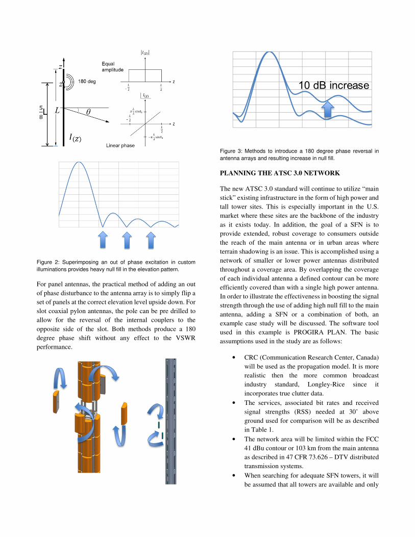
Figure 2: Superimposing an out of phase excitation in custom

illuminations provides heavy null fill in the elevation pattern.

For panel antennas, the practical method of adding an out

of phase disturbance to the antenna array is to simply flip a

set of panels at the correct elevation level upside down. For

slot coaxial pylon antennas, the pole can be pre drilled to

allow for the reversal of the internal couplers to the

opposite side of the slot. Both methods produce a 180

degree phase shift without any effect to the VSWR

performance.

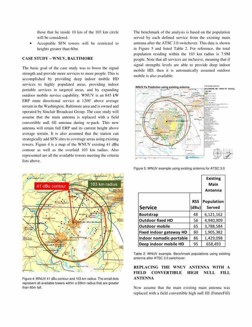
Figure 3: Methods to introduce a 180 degree phase reversal in

antenna arrays and resulting increase in null fill.

PLANNING THE ATSC 3.0 NETWORK

The new ATSC 3.0 standard will continue to utilize “main

stick” existing infrastructure in the form of high power and

tall tower sites. This is especially important in the U.S.

market where these sites are the backbone of the industry

as it exists today. In addition, the goal of a SFN is to

provide extended, robust coverage to consumers outside

the reach of the main antenna or in urban areas where

terrain shadowing is an issue. This is accomplished using a

network of smaller or lower power antennas distributed

throughout a coverage area. By overlapping the coverage

of each individual antenna a defined contour can be more

efficiently covered than with a single high power antenna.

In order to illustrate the effectiveness in boosting the signal

strength through the use of adding high null fill to the main

antenna, adding a SFN or a combination of both, an

example case study will be discussed. The software tool

used in this example is PROGIRA PLAN. The basic

assumptions used in the study are as follows:

• CRC (Communication Research Center, Canada)

will be used as the propagation model. It is more

realistic then the more common broadcast

industry standard, Longley-Rice since it

incorporates true clutter data.

• The services, associated bit rates and received

signal strengths (RSS) needed at 30’ above

ground used for comparison will be as described

in Table 1.

• The network area will be limited within the FCC

41 dBu contour or 103 km from the main antenna

as described in 47 CFR 73.626 – DTV distributed

transmission systems.

• When searching for adequate SFN towers, it will

be assumed that all towers are available and only

those that lie inside 10 km of the 103 km circle

will be considered.

• Acceptable SFN towers will be restricted to

heights greater than 60m

CASE STUDY – WNUV, BALTIMORE

The basic goal of the case study was to boost the signal

strength and provide more services to more people. This is

accomplished by providing deep indoor mobile HD

services to highly populated areas, providing indoor

portable services in targeted areas, and by expanding

outdoor mobile service capability. WNUV is an 845 kW

ERP omni directional service at 1200’ above average

terrain in the Washington, Baltimore area and is owned and

operated by Sinclair Broadcast Group. The case study will

assume that the main antenna is replaced with a field

convertible null fill antenna during re-pack. This new

antenna will retain full ERP and its current height above

average terrain. It is also assumed that the station can

strategically add SFN sites to coverage areas using existing

towers. Figure 4 is a map of the WNUV existing 41 dBu

contour as well as the overlaid 103 km radius. Also

represented are all the available towers meeting the criteria

lists above.

Figure 4: WNUV 41 dBu contour and 103 km radius. The small dots

represent all available towers within a 93km radius that are greater

than 60m tall.

The benchmark of the analysis is based on the population

served by each defined service from the existing main

antenna after the ATSC 3.0 switchover. This data is shown

in Figure 5 and listed Table 2. For reference, the total

population residing within the 103 km radius is 7.9M

people. Note that all services are inclusive, meaning that if

signal strengths levels are able to provide deep indoor

mobile HD, then it is automatically assumed outdoor

mobile is also available.

Figure 5: WNUV example using existing antenna for ATSC 3.0

Table 2: WNUV example. Benchmark populations using existing

antenna after ATSC 3.0 switchover.

REPLACING THE WNUV ANTENNA WITH A

FIELD CONVERTIBLE HIGH NULL FILL

ANTENNA

Now assume that the main existing main antenna was

replaced with a field convertible high null fill (FutureFill)

Existing

Main

Antenna

ServiceRSS

(dBu)

Population

Served

Bootstrap 48 6,121,162

Outdoor fixed HD 56 4,940,909

Outdoor mobile 65 3,788,584

Fixed indoor gateway HD 80 1,905,382

Indoor nomadic-portable 86 1,429,098

Deep indoor mobile HD 95 658,493

antenna during the re-pack process and switched to the

high null fill mode. The resulting changes in the

populations served by the defined services after increasing

the null fill by the simple conversion as described in Figure

4 are shown in Table 3.

Table 3: WNUV example. Comparison of number of people served

by each defined ATSC 3.0 service after converting to a high null fill

mode.

The results show a slight loss of 174,000 potential

consumers (indicated by the blue cells) using lower RSS

services in the outer coverage areas. It also shows a

substantial gain of 441,000 in potential consumers that may

use data intensive services in the near in coverage areas.

The data from Table 3 is plotted in Figure 6 to better

illustrate the effect of increasing the null fill.

Figure 6: WNUV example. Comparison of number of people served

by each defined ATSC 3.0 service after converting to a high null fill

mode.

ADDING SFN SITES TO THE EXISTING WNUV

ANTENNA SYSTEM

Next, the effect of strategically placing four optimized 50

kW ERP SFN sites within the limits of the FCC contour

will be analyzed. In the process, each site begins as an omni

directional azimuth pattern. Power reductions are then

performed in all directions to meet the FCC limitations.

The results predict the best theoretical azimuth pattern to

be applied at each site. Figure 7 is a map of the locations

chosen for each SFN site and Figure 8 depicts the

optimized theoretical patterns generated for each site.

Figure 7: WNUV example. Four tower locations chosen for the SFN

sites to be added to the existing main antenna to create the full

ATSC 3.0 network.

Figure 8: WNUV example. Best fit optimized theoretical azimuth

patterns chosen for each site based on power reductions to meet

FCC limits.

The effect on populations served by the previously defined

ATSC 3.0 services by adding four theoretical SFN sites to

the existing main antenna with standard null fill are listed

in Table 4 and plotted in Figure 9.

Existing

Main

Antenna

Future High

Null Fill

Converted

ServiceRSS

(dBu)

Population

Served

Population

Served

%

Change

Population

Change

Outdoor fixed HD 56 4,940,909 4,847,172 -2% -93,737

Outdoor mobile 65 3,788,584 3,716,684 -2% -71,900

Fixed indoor gateway HD 80 1,905,382 1,896,801 0% -8,581

Indoor nomadic-portable 86 1,429,098 1,527,028 7% 97,930

Deep indoor mobile HD 95 658,493 1,001,992 52% 343,499

Table 4: WNUV example. Comparison of number of people served

by each service under ATSC 3.0 when adding four SFN sites to the

existing main antenna with standard null fill.

Figure 9: WNUV example. Comparison of number of people served

by each service under ATSC 3.0 when adding four SFN sites to the

existing main antenna when standard null fill.

As seen by the data, 1,460,000 possible consumers have

been gained throughout the coverage area. Figure 9

illustrates a slight gain in consumers serviced by data

intensive services while showing a significant gain in

consumers serviced by lower bit rate services.

ADDING SFN SITES TO THE WNUV ANTENNA

CONVERTED TO HIGH NULL FILL

The next scenario to be analyzed is theoretically replacing

the existing antenna with a FutureFill field convertible

design for re-pack and adding SFN sites. Table 5 and

Figure 10 display these results.

Table 5: WNUV example. Comparison of number of people served

by each service under ATSC 3.0 when adding four SFN sites to a

new field convertible high null fill main antenna.

Figure 10: WNUV example. Comparison of number of people

served by each service under ATSC 3.0 when adding four SFN

sites to a new field convertible high null fill main antenna.

Overall, 1,640,000 new possible ATSC 3.0 consumers

have been added. This scenario results in a significant gain

in consumers serviced by both lower and higher data rate

services. From the data, a much more even distribution in

populations served by all services is observed compared to

just using the existing antenna for ATSC 3.0 delivery and

adding an SFN.

REPLACING THEORETICAL ANTENNA

PATTERNS WITH REAL DESIGNS

The next logical step in the ATSC 3.0 network planning

process is to replace the best fit theoretical azimuth patterns

generated by the planning software with real designs. A

combination of panel and slotted coaxial antenna designs

were used to replicate the theoretical patterns shown in

Figure 8. The overlay comparison is shown in Figure 1.

Figure 11: WNUV example. Real antenna design azimuth patterns

(shown in red) used to replicate the optimized theoretical azimuth

patterns (shown in blue).

Existing

Main

Antenna

Standard

Elevation

Pattern

ServiceRSS

(dBu)

Population

Served

+ SFN

Population

Served

%

Change

Population

Change

Outdoor fixed HD 56 4,940,909 5,405,598 9% 464,689

Outdoor mobile 65 3,788,584 4,189,184 11% 400,600

Fixed indoor gateway HD 80 1,905,382 2,157,756 13% 252,374

Indoor nomadic-portable 86 1,429,098 1,702,093 19% 272,995

Deep indoor mobile HD 95 658,493 734,238 12% 75,745

Existing

Main

Antenna

Future High

Null Fill

Converted

ServiceRSS

(dBu)

Population

Served

+ SFN

Population

Served

%

Change

Population

Change

Outdoor fixed HD 56 4,940,909 5,283,509 7% 342,600

Outdoor mobile 65 3,788,584 4,099,525 8% 310,941

Fixed indoor gateway HD 80 1,905,382 2,142,988 12% 237,606

Indoor nomadic-portable 86 1,429,098 1,760,761 23% 331,663

Deep indoor mobile HD 95 658,493 1,077,222 64% 418,729

Note that in most cases, the ERP had to be reduced from

50 kW to remain within the theoretical pattern footprint.

The impact of replacing the best fit theoretical patterns

with real antenna design are shown in Table 6.

Table 6: WNUV example. Comparison of number of people served

by each service under ATSC 3.0 when adding four SFN sites with

real antenna designs to a new field convertible high null fill main

antenna.

As can be seen from the data comparison between Table 5

and Table 6, with careful antenna design, a loss of only

60,000 possible ATSC 3.0 consumers out of 1,640,000 is

observed. This translates to a minimal 4% loss.

WHAT TYPE OF ANTENNAS WILL BE BEST

SUITED FOR ATSC 3.0 SFN NETWORKS

Different types of broadcast antennas have different

advantages and disadvantages. For example, slotted

coaxial pylon antennas are much smaller in size thus have

substantially less wind load then panel arrays with the same

gain. They also exhibit higher reliability due to the fact that

slotted coaxial antennas have less connections and less

parts. Another feature of slotted antennas is their pattern

versatility. Elevation patterns can be shaped by discretely

controlling the amplitude and phase emanating from each

vertical layer. The azimuth patterns can also be tailored to

meet even the most difficult coverage requirements by

changing the pipe size, the number and orientation of slots

around the pipe, the power division between those slots and

through the addition of fins and directors. The

disadvantage to slotted antennas that a slot radiator is

inherently narrow band and thus has limited channel range.

Panel antennas on the other hand are broadband and are an

excellent choice for co-located shared SFN sites. They too

exhibit excellent pattern flexibility, by varying the array

radius, number of panels around, their location and

orientation as well as their amplitude and phase. Another

choice that will be considered for future ATSC 3.0 SFN

sites are slot cavity antennas. They are basically a cross

between a panel and a slotted coaxial design, providing

panel bandwidth in a pylon package. In short, there will be

no “one size fits all” antenna solution for ATSC 3.0 SFN’s.

A combination of panel, slot and broadband slot cavity

antennas will be required.

CONCLUSION

It is clear that ATSC 3.0 services will require a new

definition of received signal strengths. By planning ahead

and through the use of innovative antenna design as well as

advanced SFN planning tools, these required signal

strengths can be achieved.

APPENDIX A

In can be shown mathematically that superimposing an out

of phase excitation approximately 5/8’s of the way from

the bottom of an array consisting of an illumination with a

constant amplitude and linear phase taper provides null fill

in the first three nulls below the main beam. If the phase

excitation at this point is 180 degrees, the starting beam tilt

is unaffected, thus meeting the goal of close-in signal

strength improvement with minimum loss in the far

regions.

A continuous source distribution can be used to

approximate linear arrays of discrete elements. The far

field pattern of a continuous line source having a uniform

amplitude and linear phase taper is given in equation (1).

Figure 1: Continuous line source with equal amplitude and linear

phase taper.

����~ ����� ����!"���!#��� ����!"���!#�

(1)

Existing

Main

Antenna

Future High

Null Fill

Converted

ServiceRSS

(dBu)

Population

Served

+ Real Ant.

SFN

Population

Served

%

Change

Population

Change

Outdoor fixed HD 56 4,940,909 5,276,767 7% 335,858

Outdoor mobile 65 3,788,584 4,095,082 8% 306,498

Fixed indoor gateway HD 80 1,905,382 2,123,632 11% 218,250

Indoor nomadic-portable 86 1,429,098 1,742,929 22% 313,831

Deep indoor mobile HD 95 658,493 1,065,715 62% 407,222

Letting

$ %& ��'(� − �'(��� (2)

���� ≈ ����+�+ (3)

The pattern maximum or beam tilt is located at � �� and

the nulls located by at x = +/-1, +/-2, +/-3,….

A point source is placed along the Z axis at location Z0 as

shown in Figure 2.

Figure 2: Point source placed along the continuous line source.

The far field pattern of the point source at point Z0 is given

by equation (4).

�,��� -./0."/1�2#� + (4)

Q is the amplitude and ϕ the offset of the feed phase of the

point source relative to the line source at the same location.

3 3,4 − 35��6�7�� (5)

In choosing the phase offset between the point source and

the line source, one must consider that the objective is to

have the beam tilt remain at � �� and be unaffected by

the addition of the point source. For this to be true the only

two choices are the point source to be in phase or 180

degrees out of phase from the line source at the point

sources location. Choosing ϕ = 180 will be considered at

this point.

The total pattern is the coherent sum of the line source and

point source and is represented by equation (6).

���� ≈ ����+�+ + -./�."/1�2#� + (6)

By placing the fields of the line source and the point source

in phase quadrature at a defined location in the far field will

ensure cancellation cannot occur and thus null fill is

obtained. The phase angle of the point source is readily

determined from the exponential of the second term in

equation (6).

9 − 29 :#

%$ (7)

Setting the point source in phase quadrature with the line

source and solving for the location of the point source to

achieve null fill centered around the first three null or x=2

produces the following result.

9 − 297�

�$ =

9

2;<$ = 2

:#

%= .125 (8)

Note that this location is .125L above the array centerline

or approximately 5/8 L from the bottom of the array.

REFERENCES

[1] “Broadcast Antenna Design to Support Future

Broadcast Technologies”, John L. Schadler, NAB BEC

Proceedings 2014.

[2] ITU-R BT.2137 Coverage predictions methods and

planning software for digital terrestrial television

broadcasting networks

[3] TV Technology: “DTV in the House, Part1”, Doug

Lung, Sept 5, 2007

[4] ITU-R BT.2033-1, “Planning criteria, including

protection ratios, for second generation of digital terrestrial

television broadcasting systems in the VHF/UHF bands”

[5] “Effect of AWGN & Fading (Rayleigh & Rician)

channels on BER performance of a WiMAX

communication System, IJCSIS, Awon, Islam, Rahman

and Islam

[6] ITU-R P.1546-5 Method for point to area predictions

for terrestrial services in the frequency range 30MHz to

3000 MHz.

Acknowledgement

A special thank you to good friend Dan Janning for his

personal help in formulating the mathematical basis to

support the null fill technique described in this paper. Dan

is currently an Electronics Engineer, AFRL/RYMD

Air Force Research Laboratory Sensors Directorate,

Multi-Spectral Sensing and Detection Division,

RF Technology Branch

The author would like to also thank Andy Whiteside and

Bill Soreth for their contributions.