Anton Peterlin and DNA

Rudolf Podgornik1

1Department of Physics, Faculty of Mathematics and Physics,

University of Ljubljana, Jadranska 19, SI-1000 Ljubljana, Slovenia

Department of Theoretical Physics (F-1),

J. Stefan Institute, Jamova 39, SI-1000 Ljubljana, Slovenia

and

Laboratory of Physical and Structural Biology, NICHD, Bld. 9 Rm. 1E-116,

National Institutes of Health, Bethesda, MD 20892-0924, USA

(Dated: July 8, 2008)

I will present an overview of Peterlin’s work on the determination of DNA persistence length by

analysing the Bunce - Doty light scattering experiments in terms of the Kratky - Porod elastic worm-

like chain model. I will describe the theory he used, the general ramifications of the experimental

method and the unavoidable limitations of his result, as well as their impact on the development of

DNA science in general.

PACS numbers:

Historic context1953 was a veritable annus mirabilis for DNA science in more respects then one.

First of all, of course, in the April 24 issue of the premier science publication Nature,the structure of DNA in dense fibers was elucidated in three fundamental and epoch-making papers: the first one by Watson and Crick [1], the second one by Franklinand Gosling [2], and the third one by Wilkins, Stokes and Wilson [3]. Their workon molecular structure of DNA launched the era of the double-helix. This scientificbreakthrough was based on one side on the detailed X-ray scattering studies of DNAfibers, prepared from calf thymus DNA by the Swiss scientist Rudolf Signer, startedby William Astbury in 1937, picked up by Maurice Wilkins in 1951 and culminating in1952 with the iconic Photo 51 obtained by Rosalind Franklin and Raymond Gosling.The interpretation and the reading of these diffractograms was based heavily on thetheory of the scattering intensity of helical molecules devised in 1951 by W. G. Cochran,F. Crick and V. Vand [4] (the CCV theory). Though the original aim of the CCV theorywas to provide a theoretical foundation for the elucidation of the structure of helicalproteins, such as the alpha helix discovered in 1952 by L. Pauling, it turned out that itcould be profitably applied also to the X-ray scattering of DNA. In particular it helpedto associate the broad features of the DNA diffractograms with the physical parametersof the helix, as well as to elucidate the fingerprint of the double helical, assymetricalnature of this helix, in the diffraction intensity.

The rest is history one would be inclined to say, were it not for the other discoverypublished in the same journal in the very same year, about two - actually in theFebruary 7 issue - months before the papers on the double-helical nature of DNA. Thepaper I am referring to was submitted on June 5 the previous year and is entitledLight Scattering by very Stiff Chain Molecules [5], authored by Anton Peterlin, thenthe director of the ”Jozef Stefan” Institute of Physics in Ljubljana [30]. Peterlin wasanalysing the experimental data on light scattering of dilute DNA aqueous solutions and

2

was applying the theory of light scattering to the DNA solution case, in the same waythat Watson and Crick were applying the theory of X-ray scattering of helical moleculesto the case of DNA fibers. The light scattering experiments on DNA solutions, orthymonucleic acid solutions as they were refferred to at that time, were performed byBarbara H. Bunce [31], who in 1950-1951 worked as a National Institutes of HealthPredoctoral Fellow in the lab of Paul Doty [32], the founder of the Department ofBiochemistry and Molecular Biology at Harvard. P. Doty, together wit Bruno Zimmand Herman Mark, co-authored the seminal paper on determining absolute molecularweights of polymers by light scattering [6] and was interested in the physico-chemicalcharacterisation of macromolecules in general [7]. Thus his Ph.D. student B. H. Bunce[8] used in particular the light scattering methods to determine molecular weight ofDNA in aqueous solutions. They published their work in 1952 in two papers, one inJournal of the American Chemical Society and the other one in the Journal of PolymerScience [9].

In order to learn anything from the light scattering experiment on DNA aqueoussolutions, of the type performed by Bunce and Doty, one has to evaluate the corre-sponding scattering function based on a molecular model of DNA, and compare it towhat is seen in experiments. In particular Peter J. W. Debye, when at Cornell but alsoafter his retirement in 1952, was using his early work on X-ray scattering and applyingit to the determination of molecular weight of polymer molecules in solution. In hisevaluation of the scattering function or the form factor of a polymer chain in a solution,he used the random walk or the Gaussian chain model to describe the thermal statisticsof a completely flexible polymer molecule [10]. A few years before, in 1949, O. Kratkyand G. Porod presented their worm-like chain model of a polymer [11] which was sup-posed to describe semi-flexible polymers that show persistence in the direction of thechemical bonds. Otto Kratky is among the towering figures in the theory and design ofX-ray scattering experiments. In 1940 he became the director of the X-ray departmentof the Kaiser-Wilhelm institute in Berlin and in 1943 he was appointed as professorat the Institute of physical chemistry in Prague, moving three years later to Graz as aprofessor of theoretical and physical chemistry. His most acknowledged research effortswere in the development of X-ray small-angle scattering methods, especially measure-ments of thermodynamic properties of polymers and biopolymers. From 1972 he wasthe head of the Institut fur Rontgenfeinstrukturforschung der Akad. d. Wiss. und

des Forschungszentrums Graz. Gunther Porod studied physics and chemistry underKratky and was Kratky’s most important coworker in X-ray small angle scattering. In1965 he was appointed as professor of experimental physics at the University of Graz.

Around 1952 Peterlin had the idea that DNA should be much closer to the Kratky-Porod semi-flexible chain model then to the Debye’s Gaussian chain model, appropriatefor other, less locally stiff polymers. He thus used the Kratky-Porod model to evaluatethe form factor of a long polymer chain. As we know today, this problem has acomplicated analytical solution, but at that time Peterlin had to use an approximateapproach in order to calculate it.

I will not say more about the particular circumstances of Peterlin’s life at that time,since they will be covered by other contributors to this volume.

In what follows I will first present a modern view of the Kratky-Porod model, andevaluate the two limiting forms of the polymer form factor that follow from this model.

3

Then I will discuss the way Peterlin approached this problem and how he analysedDNA light scattering data of Bunce and Doty in 1953. I will conclude with an outlookon the DNA work of Peterlin and its historical impact [33].

A. The Kratky-Porod model

First I will derive the Kratky-Porod model in its modern form and calculate theensuing form factor of a polymer chain in a solution. Let us consider the polymerchain as a torsionally relaxed elastic filament, whose elastic energy does not dependon the torsional deformation. For a filament with a circular cross section one canwrite the elastic deformation energy in the form of an Euler-Kirchhoff elastic filamentdeformation energy as [12]

F = 12Kc

∫ L

0

t2d` = 12Kc

∫ L

0

(dtd`

)2

d`, where t = r(`) (1)

is the unit tangent vector of the polymer described with a parametric curve r = r(`),with ` the natural parameter, i.e. the arc-length. The expression for the deformationenergy looks similar to kinetic energy of a particle with ”position” t and ”time” `,which is the essence of the Kirchhoff kinematic analogy [13]. In addition this partclewould have to move on a unit sphere since t2 = 1. For an elastic filament that is ata constant non-zero temperature one should study its free energy as opposed to itsenergy. It can be obtained from the partition function that is defined as

Z =∫{t(`)}

D[t(`)] e−12βKc

R L0 ( dt

d` )2d` with t2(`) = 1. (2)

where β is the inverse thermal energy, 1/β = kBT and the integral has to be performedover all unit vector configurations {t(`)}. This partition function is formally analogousto the probability amplitude Z(t2(L), t1(0)) of a quantum mechanical particle living ona unit sphere, for a final ”velocity” t2(L) after ”time” L if it starts off with a ”velocity”t1(0), if one furthermore identifies the length of the filament with ”imaginary time”[14]. The formal relationship can be written as

Z =∫dt1

∫dt2Z(t2(L), t1(0)). (3)

One can thus derive an equation for the ”probability amplitude” Z(t2(L), t1(0)) anal-ogous to the Schrodinger equation in the form

∂Z(t2(L), t1(0))∂L

=1

2LpL2Z(t2(L), t1(0)), (4)

where Lp = βKc is introduced as the persistence length and L2 is the angular part ofthe Laplace operator, given by

L2 =1

sin θ∂

∂θ

(sin θ

∂

∂θ

)+

1sin θ2

∂2

∂φ2. (5)

4

Since the filament looks statistically the same along all of its contour one can assumethe ansatz of homogeneity and write

<t(`2) · t(`1)> = <t(`2 − `1) · t(0)> = <cos θ(`2 − `1)>. (6)

If we now take note of the statistical definition of <cos θ(`2 − `1)> [34] we can derivestraightforwardly that

∂<cos θ(`2 − `1)>∂L

=1

2Lp<L2 cos θ(`2 − `1)> = − 1

Lpcos θ(`2 − `1). (7)

The last equality follows from the fact that L2 is the angular part of the Laplaceoperator and thus that L2 cos θ(`2 − `1) = −2 cos θ(`2 − `1). Therefore one obtainsthat

<cos θ(`2 − `1)> = e−(`2−`1)/Lp . (8)

The directional correlations along an elastic filament decay exponentially, with a decaylength equal to the persistence length. The persistence length is thus the correlationlength for elastic correlations along the filament. This can be seen straightforwardlyfrom the length of the chain directed along the direction of the beginning of the chaini.e.

<t(0) · (R(L)−R(0))> = <t(0) ·

(∫ L

0

t(`′)d`′)> =

∫ L

0

e−`/Lp d`′ =

= Lp(

1− e−L/Lp

). (9)

Here we have taken into account that R(L)−R(0) =∫ L0

dr(`)d` d` =

∫ L0

t(`)d`. For longfilaments the length of the chain directed along the direction of the beginning of thechain thus saturates at the value of the persistence length.

We are now in a position to calculate what is the statistical shape of an elasticfilament in a brownian thermal bath. Let us just remind ourselves that the averagesquare of the end to end separation of the filament is given by

<(R(L)−R(0))2> =∫ L

0

∫ L

0

d`d`′<dr(`)d`

dr(`′)d`′

> =

=∫ L

0

∫ L

0

d`d`′<t(`)t(`′)> =

=∫ L

0

∫ L

0

d`d`′<cos θ(`− `′)>. (10)

Using now Eq. 8 for the angular average we remain with

<(R(L)−R(0))2> = 2Lp(L− Lp + Lpe−L/Lp

). (11)

For small values of the length of the chain, L/Lp � 1, it thus behaves as a stiff rod,whereas in the opposite limit, L/Lp � 1, it behaves as a convoluted Gaussian chain.For more complete description of the two limits, see below. The two limiting behaviorsof the Kratky-Porod model are schematically presented on Fig. 1.

5

FIG. 1: Statistical shape (exaggerated) of an elas-

tic filament in the Kratky-Porod model. Short fil-

aments really look like stiff rods. The longer they

are, the more convoluted they become, eventually

becoming completely disordered Gaussian chains.

This general result was first de-rived by Kratky and Porod in 1949,be it in a completely different fash-ion, and thus the model of an elas-tic filament based on their calcu-lation is usually referred to as theKratky-Porod model or the worm-like chain model or the semiflexiblechain model, the nomenclature reallyvaries with the author.

The essence of the Kratky-Porodmodel is that there are persistentorientational correlations along thechain that die out exponentiallyalong the contour length of thechain, see Eq. 8, with a character-istic length equal to the persistencelength of the chain. Equivalently onecould claim that within this modelthe orientation of the first link in the

chain is preserved along the length of the chain again equal to its persistence length,see Eq. 9. The closed form expressions that we derived above have some very intuitivelimiting forms that we discuss next.

B. The limiting forms of the Kratky-Porod model

The Kratky-Porod model has two important limits depending on the ratio L/Lp thatwe shall analyze in detail in what follows. They are imbedded in the Kratky-Porodmodel but can be derived even without invoking it. First of all we have the Gaussianchain limit, that can be derived as

limL/Lp−→∞

<(R(L)−R(0))2> = 2LpL, (12)

The length 2Lp is usually referred to sa the Kuhn length and describes the independentunit of the polymer chain. Obviously in this limit the thermal bath completely destroysthe correlations between far away segments along the filament.

This result can be obtained also from a simplified consideration along the followinglines. Assume the chain is composed of segments of length b directed along the localtangent t(`), so that the end-to-end vector is defined as

R(L)−R(0) =∫ L

0

t(`) d`.

The segments are assumed to be orientationally completely uncorrelated so that

<t(`) · t(`′)> = b δ(`− `′). (13)

6

This definition of the orientational correlation function gives for the length of the chaindirected along the direction of the beginning of the chain i.e.

<t(0) · (R(L)−R(0))> = <t(0) ·

(∫ L

0

t(`′)d`′)> = b

exactly the length of the segment b. It follows straightforwardly in this case that theaverage size of the chain squared is

<(R(L)−R(0))2> = b

∫ L

0

∫ L

0

δ(`− `′) d`d`′ = b L. (14)

Clearly by comparing Eqs. 12 and 14 we can identify the Kuhn length with the lengthof the statistically independent unit of the polymer chain, thus b = 2Lp.

The other limit of the general Kratky-Porod result can be derived for a very stiff ora very short chain in the form

limL/Lp−→0

<(R(L)−R(0))2> = L2, (15)

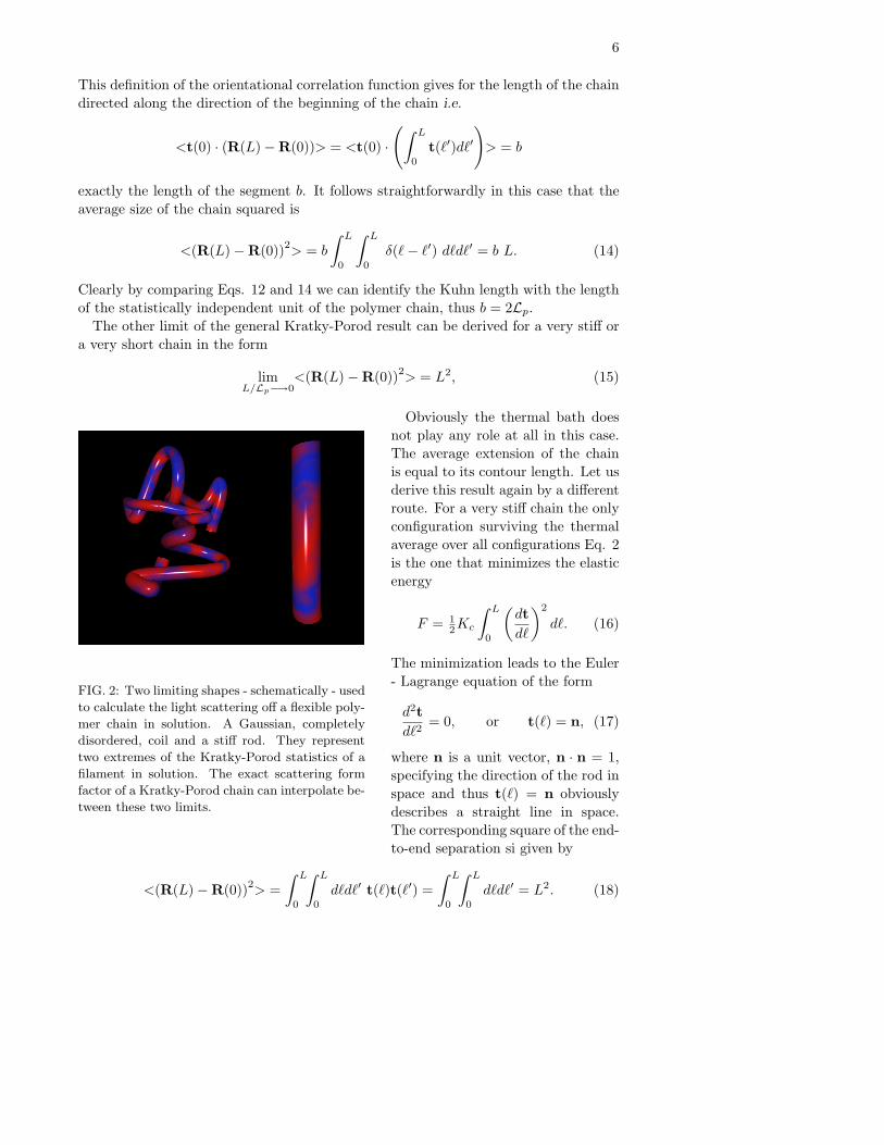
FIG. 2: Two limiting shapes - schematically - used

to calculate the light scattering off a flexible poly-

mer chain in solution. A Gaussian, completely

disordered, coil and a stiff rod. They represent

two extremes of the Kratky-Porod statistics of a

filament in solution. The exact scattering form

factor of a Kratky-Porod chain can interpolate be-

tween these two limits.

Obviously the thermal bath doesnot play any role at all in this case.The average extension of the chainis equal to its contour length. Let usderive this result again by a differentroute. For a very stiff chain the onlyconfiguration surviving the thermalaverage over all configurations Eq. 2is the one that minimizes the elasticenergy

F = 12Kc

∫ L

0

(dtd`

)2

d`. (16)

The minimization leads to the Euler- Lagrange equation of the form

d2td`2

= 0, or t(`) = n, (17)

where n is a unit vector, n · n = 1,specifying the direction of the rod inspace and thus t(`) = n obviouslydescribes a straight line in space.The corresponding square of the end-to-end separation si given by

<(R(L)−R(0))2> =∫ L

0

∫ L

0

d`d`′ t(`)t(`′) =∫ L

0

∫ L

0

d`d`′ = L2. (18)

7

Here we have ignored the thermal average since as we noted for a very stiff chainthe only possible configuration is the one corresponding to the solution of the Euler-Lagrange equation Eq. 17. The statistical average thus reduces to a single value. Inthis limit the elastic properties of the chain obviously do not figure any more in itsstatistical description. A shematic representation o fthe two limits of the Kratky-Porodchain are presented on Fig. 2.

C. Light scattering from a Kratki-Porod filament in solution

We now move to the most important consequence of the Kratky-Porod model thatwas investigated and used by Peterlin in his analysis of X-ray scattering data on DNAsolutions. Let us start from a definition of the total scattering intensity as the averageof the square of the structure factor of a polymer filament in solution which is given by

I(Q) = <|F(Q)|2> (19)

since we have to avaluate the statistical average <. . .> over all the conformations ofthe filament in solution. Assuming that the filament is infinitely thin, and thus doesnot posses any transverze dimension, this leads to

I(Q) = <|F(Q)|2> = <

∫(V )

ρ(r) eiQ·r d3r∫

(V )

ρ(r′) e−iQ·r′d3r′>

=1L2

∫ L

0

∫ L

0

<eiQ·(r(`)−r(`′))> d`d`′. (20)

Here we have conventionally normalized the result by dividing it with L2. It is verydifficult to calculate this quantity exactly for the Kratky-Porod chain, though there isno shortage of approximate results that interpolate between two obvious limiting casesgiven by Eqs. 14 and 18. Let us evaluate these limits explicitly.

For a Gaussian chain the probability distribution of segments with length r(`)−r(`′)is Gaussian due to the central limit theorem that follows from statistical independenceof the segments. For a Gaussian distribution one can furthermore derive [15]

<eiQ·(r(`)−r(`′))> = e−12<(Q·(r(`)−r(`′)))2

>. (21)

We already know that the statistics of a Gaussian chain is isotropic, which means thatfor each Cartesian component xi one can write

<(xi(`)− xi(`′))2> = 13b|`− `

′|.

where of course we took account of the fact that <(r(`)−r(`′))2> = b|`−`′|. Thereforewe finally remain with

I(Q) =1L2

∫ L

0

∫ L

0

e−b6Q

2|`− `′| d`d`′ =2(e−(QRg)2 − 1 + (QRg)2)

(QRg)4= f((QRg)2),

where f(x) is the Debye scattering function and the radius of gyration Rg is given byR2g = 1

6 bL. The Debye scattering function can be often conveniently approximated by

I(Q) =1

1 + 12Q

2R2g

8

with about 15 % accuracy for the whole range of Q values. Debye derived this scatteringfunction within the random walk model of a polymer chain, that accurately describesthe thermal statistics of a completely flexible polymer molecule with only short rangeorientational correlations along the chain. The opposite limit within the Kratky-Porod

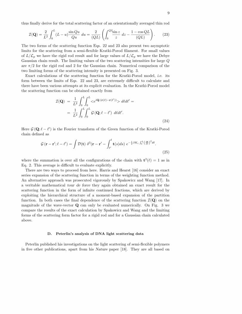
FIG. 3: Exact scattering intensity for a Kratki-Porod chain calculated by Spakowicz and

Wang (Adapted from A.J. Spakowicz and Z-G. Wang, J. Chem.Phys. 37 (2004) 5814-5823).

The l.h.s. graph shows (kL)I(k) as a function of the dimensionless wave vector k = 2LpQfor different values of the dimensionless length of the chain N = L/(2Lp). (in this work

the symbol S(Q) is used instead of I(Q)). N = 0.1 (solid line), N = 0.5 (dashed line) and

N = 1 (dashed-dotted line). For comparison the figure also includes the rigid rod result Eq.

23 (dotted line). The r.h.s. graph shows (kL)I(k) for N = 100 for the exact form of the

Kratky-Porod scattering function (solid line) and the Gaussian chain (dashed curve). The

Kratky - Porod model closely agrees with the Gaussian chain model for small k; however, as k

increases, these two models diverge. Since a wormlike chain is rigid at sufficiently small length

scales, the structure factor for the wormlike chain model approaches the rigid rod limit for

large k regardless of the stiffness of the chain. Such behavior is not captured by the Gaussian

chain model since it has no (bending) stiffness at any length scales.

model is again obtained by treating the filament to the lowest order as a rigid rod.In this case r(`) − r(`′) = n(` − `′). where n is the constant unit direction tengentialvector of the rod. For the rod the statistical average is translated directly into theintegral over all the orientations of the rod with respect to Q. Thus we remain with

I(Q) =1L2

∫ L

0

∫ L

0

<eiQ·(r(`)−r(`′))> d`d`′

=1L2

∫ L

0

∫ L

0

eiQ|`−`′| cos θd(cos θ) d`d`′ =

2L2

∫ L

0

∫ L

0

sinQ|`− `′|Q|`− `′|

d`d`′.

(22)

One can now introduce an auxiliary variable u = ` − `′. The domain of integrationdecomposes into a stripe from u to L for the variable ` and from 0 to L for u. We can

9

thus finally derive for the total scattering factor of an orientationally averaged thin rod

I(Q) =2L2

∫ L

0

(L− u)sinQuQu

du =2

(QL)

(∫ QL

0

sin zz

dz − 1− cosQL(QL)

). (23)

The two forms of the scattering function Eqs. 22 and 23 also present two asymptoticlimits for the scattering from a semi-flexible Kratki-Porod filament. For small valuesof L/Lp we have the rigid rod result and for large values of L/Lp we have the DebyeGaussian chain result. The limiting values of the two scattering intensities for large Qare π/2 for the rigid rod and 2 for the Gaussian chain. Numerical comparison of thetwo limiting forms of the scattering intensity is presented on Fig. 3.

Exact calculations of the scattering function for the Kratki-Porod model, i.e. itsform between the limits of Eqs. 22 and 23, are extremely difficult to calculate andthere have been various attempts at its explicit evaluation. In the Kratki-Porod modelthe scattering function can be obtained exactly from

I(Q) =1L2

∫ L

0

∫ L

0

<eiQ·(r(`)−r(`′))> d`d`′ =

=1L2

∫ L

0

∫ L

0

G (Q; `− `′) d`d`′.

(24)

Here G (Q; `− `′) is the Fourier transform of the Green function of the Kratki-Porodchain defined as

G (r− r′; `− `′) =∫D(t) δ3(r− r′ −

∫ `

`′t(s)ds) e−

12βKc

R L0 ( dt

d` )2d`.

(25)

where the summation is over all the configurations of the chain with t2(`) = 1 as inEq. 2. This average is difficult to evaluate explicitly.

There are two ways to proceed from here. Harris and Hearst [16] consider an exactseries expansion of the scattering function in terms of the weighting function method.An alternative approach was prosecuted vigorously by Spakowicz and Wang [17]. Ina veritable mathematical tour de force they again obtained an exact result for thescattering function in the form of infinite continued fractions, which are derived byexploiting the hierarchical structure of a moment-based expansion of the partitionfunction. In both cases the final dependence of the scattering function I(Q) on themagnitude of the wave-vector Q can only be evaluated numerically. On Fig. 3 wecompare the results of the exact calculation by Spakowicz and Wang and the limitingforms of the scattering form factor for a rigid rod and for a Gaussian chain calculatedabove.

D. Peterlin’s analysis of DNA light scattering data

Peterlin published his investigations on the light scattering of semi-flexible polymersin five other publications, apart from his Nature paper [18]. They are all based on

10

his approximate treatment of the scattering integral Eq. 20 that he was not able toevaluate exactly. The explicit and exact evaluation of the scattering function within theKratky - Porod model was evaluated later by Harris and Hearst as well as Spakowitzand Wang (see above). Peterlin writes Eq. 20 in the form

I(Q) =1L2

∫ L

0

∫ L

0

<eiQ·(r(`)−r(`′))> d`d`′ =

=1L2

∫ L

0

∫ L

0

e−12<(Q · (r(`)− r(`′)))2> d`d`′ =

=1L2

∫ L

0

∫ L

0

e−Q2

6 <(r(`)−r(`′))2> d`d`′. (26)

by implementing the Gaussian ansatz Eq. 21 and the fact that the statistical distribu-tion of the polymer chain is isotropic. The magnitude of the scattering wave vector Qin the above formula is given by

Q2 =(

2πλ

2 sinθ

2

)2

,

with λ the wavelength of light and θ the scattering angle. The difficult part in theabove integration is to get the appropriate form of <(r(`) − r(`′))2> in the Kratky-Porod model. Note that here the arguments ` and `′ do not belong to the beginningand the end of the chain, but to intermediate positions. and so the Kratky-Porod resultEq. 11 can not be used directly. One can either evaluate it explicitly and remain witha complicated integration, or one can come up with some suitable approximation andhopefully evaluate the integral analytically. It was the latter path that was pursued byPeterlin.

The approximation embraced by Peterlin on purely intuitive grounds was to take

<(r(`)− r(`′))2> = 2Lp2(u− 1 + e−u

), (27)

with x the ratio of the separation between the segments r(`), r(`′) along the chain andits persistence length, i.e. u = |` − `′|/Lp. The essence of the Peterlin approximationwas to use the Kratky-Porod form of the end-to-end separation of the chain also for thelocal segment-to-segment separation among any two segments along the chain. Thoughthis is not valid exactly, it is certainly plausible. Peterlin never explored systematicallythe range of validity of this approximation, he does however state [19] that the statis-tical deviation from this result, expected for a Kratky - Porod chain, should have littleconsequences on his final conclusions. In his opinion the local approximate relation Eq.27 should be the more accurate the larger the ratio L/Lp.

Taking this closed form expression for <(r(`)− r(`′))2> the two integrals in Eq. 26can now be evaluated analytically, yielding the following closed form expansion for thescattering intensity

I(Q) = P (p, x) = e−u[F (p, x)− p

1!F (p+ 1, x) +

p2

2!F (p+ 2, x) + . . .

](28)

Here we used the following abbreviations

p = 13

(4πλLp)2

sin2 θ

2and F (p, x) =

2(px)2

(px− 1 + e−px

),

11

where x = L/Lp. As shown by Peterlin the above scattering intensity reduces directlyto the Debye result valid for a Gaussian chain and corresponding to the limit x −→∞as

limx−→∞

P (p, x) =2w2

(w − 1 + e−w

)with w = 1

6

(4πλR

)2

sin2 θ

2,

which is the Debye result with R2 the average square end-to-end distance for a Gaussianchain.

Since experimentalists usually plot the scattering data in terms of the s.c. Zimmplots, where one plots not the scattering intensity but rather its inverse as a functionof sin2 θ

2 . Peterlin thus rewrote his results in an alternative form that would be inaccord with this convention. He thus evaluated the expansion of the inverse scatteringintensity, noticing that the Zimm plot should show a convex curvature close to theorigin for a Gaussian chain and should show a concave curvature for a stiff rod. Hisresults should fall right somewhere in between these two limits. He derived the followingform for the inverse scattering intensity

1P (p, x)

= 1 +p

3 1![x+ 3(F (1, x)− 1)] + . . . . (29)

This form is obviously linear in p = 13

(4πλ Lp

)2 sin2 θ2 and its L dependent coefficient,

i.e. [x+ 3(F (1, x)− 1)], should be easily extractable from the Zimm plot. Peterlinalso checked the limiting forms of this expression. First of all he writes down again theDebye limit of a Gaussian chain which now has the form of

limx−→∞

1P (p, x)

= 1 +w

3+ . . . again with w = 1

6

(4πλR

)2

sin2 θ

2. (30)

Here again R2 is simply the mean square end-to-end separation of a Gaussian chain.Then he derives also the form of the Zimm plot for a stiff rod. This limit corresponds tothe general case of small length of the chain in comparison with its persistence length.Formally this limit is obtained by taking x −→ 0 in the general formula Eq. 28 yieldingthe following expression

limx−→0

1P (p, x)

=(QL)

2

(∫ QL

0

sin zz

dz − 1− cosQL(QL)

)−1

= 1 +y

9+ . . . , (31)

with

y =(

4πλL

)2

sin2 θ

2,

which is completely in accord with Eq. 23. He notes that in the Zimm plot for allx his scattering curves remain concave. After obtaining the scattering intensity fora semi-flexible chain, which incidentally were calculated numerically by Mrs. Bibi-jana Cujec - Dobovisek of the J. Stefan Institute, Peterlin started comparing them toexperiments by Bunce and Doty, which were the only ones at that time involving DNA.

12

FIG. 4: Comparison between theory and experiment for

a set of DNA data. Taken from A. Peterlin, Lichtzer-

streuung an ziemlich gestreckten Fadenmolekulen, Die

Makromolekulare Chemie 9 244-268 (1953). Instead of

plotting v ∼ sin2 θ2

on the abscissa, he chose to plot log v.

Other five papers by Peterlin on the same topic contain

partial versions of this figure, showing only some, not all,

sets of data presented above.

He took the data fromBunce’s thesis and obtaineda graph showing the com-parison between theory andexperiment, see Fig. 4. Dif-ferent variants of this graphappear in several of Peter-lin’s papers dedicated to thescattering of light in diluteDNA solutions. They varyonly in regard to which datasets Peterlin chose to includein the graph. The graphpresented in the Nature paper[5] contains only data setsby Singer, Bunce-Geiduschek,Bunce-Geiduschek I andGulland. The paper in Die

Makromolekulare Chemie

[18] contains the data setsby Singer, Bunce-Geiduschek,Bunce-Geiduschek I andGulland, Bunce-GeiduschekII, Bunce-Geiduschek III,Varin I, Varin II (pH = 2.6)and Varin III. The last threedata sets were not obtainedby Bunce [20]. The paperin the Annals of the New

York Academy of Science [18] contains data sets by Singer, Bunce-Geiduschek,Bunce-Geiduschek I and Gulland, Bunce-Geiduschek II, and Bunce-Geiduschek III.The paper in the Journal of Polymer Science [18] contains only theoretical calculations,while the paper in Prog. Biophys. Mol. Bio. [18] contains data sets by Singer,Bunce-Geiduschek, Bunce-Geiduschek I and Gulland, Bunce-Geiduschek II, andBunce-Geiduschek III. The paper in Die Makromolekulare Chemie thus representsthe most thorough set of experimental data and their comparison with Peterlin’stheoretical calculations.

Obviously all the experimental data on Fig. 4 fall between the Debye Gaussian resultand the stiff rod result, indicated by the values of x =∞ and x = 0.

Peterlin now used his expression Eq. 29 and fitted the length of the chain L as wellas the persistence length Lp to the data. One should note here that the experimentaldata were not obtained for monodisperse DNA solutions and thus the length estimateshould be considered as a polydispersity average. He assembled all his results in atable. There are different variants of this table in the various papers referred to above,the most thorough one again exhibited in the Die Makromolekulare Chemie paper. Inthese tables he presents the molecular mass of the DNA used in the data set, the fitted

13

persistence length, the fitted length, the average end-to-end separation obtained fromthe fitted values of the persistence length and the total length of DNA, and the linearmass of the DNA molecule obtained as the ratio between the molecular mass and fittedDNA length. The average persistence length of DNA obtained by Peterlin is thus given

Data set DNA preparation M × 10−6 Lp[nm] L[nm] R[nm] M/L[M/0.1 nm]

1 Signer 6.7 28.5 4300 490 156

2 Bunce-Geiduschek 4 26 2600 370 154

3 Gulland 4 40 1000 280 400

4 Bunce-Geiduschek I 2.64 40 1000 280 264

5 Bunce-Geiduschek II 2.1 37 1100 280 190

6 Bunce-Geiduschek III 2.7 54 1080 340 250

7 Varin I 7.7 60.6 2100 500 370

8 Varin II (pH=2.6) 7.7 ∞ 2800 280 2750

9 Varin III 7.7 39 2820 470 270

TABLE I: Fitted persistence length, length, coil size (obtained from the Kratky-Porod formula

Eq. 11) and linear mass of the various sets of DNA data in light scattering experiments. This

table is taken from A. Peterlin, Lichtzerstreuung an ziemlich gestreckten Fadenmolekulen, Die

Makromolekulare Chemie 9 244-268 (1953). Other papers by Peterlin analysing the DNA light

scattering data contain partial versions of this table. The polydispersity of DNA samples is

not indicated. Data set 8 has a very short range and can only be fitted as a stiff rod, indicated

by the value ∞ for Lp. This data set is thus not counted in the statistics for the values of Lp.The anomalously high linear density of the data set 8 is probably due to the self-association of

DNA molecules in very acid (pH=2.6) ionic solutions. The chemical value of the linear mass

density is around 100 [M/0.1 nm].

by

Lp = 40.6 (1± 0.28)[nm] or approximately 120 base pairs, (32)

where the contour length of the base pair is taken standardly as 0.34 nm. This makesDNA a moderately stiff molecule. The Peterlin value is indeed very close, but somewhatsmaller, then the modern accepted value [21] of 46 − 50 nm or 140 − 150 base pairs,thus very close to the length of the nucleosomal DNA fragment. However, as it hasbeen realized for a while [22], it depends crucially on the ionic solution conditions andcan vary significantly with these conditions [? ]. The most accurate values for DNApersistence length are obtained from atomic force spectroscopy (AFM) [24] which isthe modern method of choice for measuring elastic properties of single macromolecules.

E. Historic impact

The number of citations of Peterlin’s six papers on the persistence length determi-nation of DNA amounts to only 185 [35] in the years following 1970. For the yearsprevious to that, I was not able to obtain any citation data but I would assume it is safe

14

to conclude that Peterlin’s work on the persistence length of DNA was not widely ap-preciated. I do not find this particularly surprising since it was tailgating the veritableexplosion of molecular biology that sprung from the epoch-making paper by Watsonand Crick published in the very same year as the Nature paper by Peterlin.

It was only much later that measurements of persistence length of DNA becamefashionable. This timeframe coincides almost exactly with the introduction of the newexperimental method of optical tweezers into the physics of single molecules. Busta-mante and his coworkers [25] in a remarkable series of physical manipulation exper-iments on DNA since 1992 made the DNA persistence length respectable again andlaunched it into the forefront of the single molecule physics. By measuring the forcevs. extension curves for a single DNA molecule, chemically attached by one end to aglass surface and by the other end to a magnetic bead, they verified that the randomthermal flopping of about 100-kb [36] double helix led to an ”entropic elasticity”, con-sistent over a thousand-fold range of force, with the elastic equation of state obtainedfrom the Kratky-Porod model, also used by Peterlin in his extraction of the persistencelength from light scattering experiments. They found out that it took about 0.1 pNto pull the ends of a DNA apart a distance of half its contour length. This 0.1 pNforce scale comes from the energy associated with a thermally excited degree of free-dom divided by the DNA persistence length, the contour length of DNA over whicha single appreciable bend occurs. The main conclusion of this work is that for smallstretching forces (double stranded) DNA behaves as a linear spring with a Hookes con-stant kDNA = 3kBT/2LpL, that is, inversely proportional to the length of the molecule(L) and its persistence length Lp. A 10 µm DNA molecule, for example, has a springconstant of approximately 10−5 pN/nm.

This atomic force spectroscopy, as it came to be referred to, thus uses the samephysics as Peterlin’s analysis, except that it does not describe the scattering propertiesof light of a Kratky - Porod chain, but its elasticity. Bustamante and coworkers wereable to fit the Kratky - Porod elastic equation of state derived by Marko and Siggia [26]with a persistence length of 50 nm, which is very close to the Peterlin’s value. Laterthese experiments were repeated at various ionic conditions of the bathing solutionleading to the measurement of a variation in the persistence length with e.g. ionicstrength of the solution [27].

The Kratky - Porod wormlike chain model thus provided the means of accuratedetermination of the persistence length of DNA from both the light scattering as wellas force spectroscopy experiments. With the advent of the force spectroscpy the lightscattering technique of persistence length determination was out of date, since theformer gives a much better accuracy and does not have any drawbacks of the lightscattering method. Recently however, Philip Nelson of the University of Pennsylvaniaand colleagues used high-resolution AFM to critically assess the applicability of theKratky - Porod model to DNA in such contexts as how it recognizes and binds toother molecules, e.g. proteins, and also for the way it packs into cellular componentsor viral capsids [28]. In all these cases DNA has to bend substantially, contrary to softthermally induced local bending that guides its behavior in light scattering or forcespectroscopy experiments. In a series of experiments [29] they came to a conclusionthat on a very short scale DNA is a lot more bendable then suggested previously bythe Kratky - Porod model. Nelson and colleagues used high-resolution AFM to image

15

the curvature in a large number of double-stranded DNA molecules over distancesas short as 5 nm, about ten times less then the scale set by the persistence length.The molecules in their experiments were gently adsorbed onto a negatively chargedmica surface with the help of small concentrations of MgCl2. When they analysed thestatistical frequency of various DNA conformations in the AFM images, the number ofhighly bent segments was much greater than predicted by the Kratky - Porod model.Their analysis on these length scales suggests that DNA elasticity in general does notfollow Hookes law. Moreover, they were able to fit their data to a new general modelthat they have named the sub-elastic chain model which differs radically from theKratky - Porod model.

The fact that the elastic energy at length scales much shorter than the persistencelength does not obey Hooke’s law and thus can not be described by the Kratky - Porodmodel does not disqualify it for describing light scattering or force spectroscopy exper-iments on single DNA molecules. On the length scales probed by these mathods, thedetails of the elastic properties of the segments are washed out by thermal fluctuations,and the molecule as a whole follows the predictions of the Kratky - Porod model. Atmuch smaller scales, however, the effect of thermal fluctuations is small and it is possi-ble to observe nonlinear elasticity that is not captured by the Kratky - Porod model. Insolid and soft matter, there are numerous examples of effective energies depending onthe length scale at which they are studied, so it is no surprise to find similar behaviourin semiflexible molecules such as DNA. The new model of DNA elasticity proposed byNelson et al. implies that the elastic restoring force is constant when the molecule isbent on small length scales and is not proportonal to the local curvature as impliedby the Kratky - Porod model. The constancy of restoring forces in this experimentis apparently a consequence of the thermodynamic equilibrium between two types ofdifferently stretched links. In a similar fashion, the small-length-scale bending of DNAobserved and quantified by Nelson et al. could be due to an equilibrium between DNAmolecules with different values of the local bend angle.

One could thus conclude that Peterlin’s breakthrough determination of DNA per-sistence length in 1953 was overshadowed by the birth of molecular biology, while thepossible stronger impact of his work in later years was sidetracked by the introductionof new experimental techniques that gave not only a much more accurate value of thepersistence length, but also elucidated the limits of the elastic model of DNA used sosuccessfully by Peterlin. Nevertheless it should not be forgotten that he was the firstone to come up with a reliable value for DNA persistence length that withstood thetest of time.

F. Acknowledgments

I would like to thank Prof. Dr. Peter Laggner, Managing Director at the Instituteof Biophysics and Nanosystems Research of the Austrian Academy of Sciences, Graz,and Doc. Dr. Georg Pabst, Institute of Biophysics and Nanosystems Research of theAustrian Academy of Sciences, Graz for providing me with historical data on Kratky,

16

Porod and Peterlin.

[1] J. D. Watson and F. H. C. Crick, Molecular structure of Nucleic Acids, Nature 171

737738 (1953).

[2] R. Franklin and R. Gosling, R., G. Molecular Configuration in Sodium Thymonucleate,

Nature 171 740-741 (1953).

[3] M. H. F. Wilkins, A.R. Stokes A.R. and H. R. Wilson, Molecular Structure of Deoxypen-

tose Nucleic Acids, Nature 171 738-740 (1953).

[4] W. Cochran, F.H.C. Crick and V. Vand, The Structure of Synthetic Polypeptides. I. The

Transform of Atoms on a Helix, Acta Cryst. 5 581-586 (1952).

[5] A. Peterlin, Light Scattering by very Stiff Chain Molecules, Nature, 171 259-260 (1953).

[6] P.M. Doty, B.H. Zimm and H. Mark, An investigation of the determination of molecular

weights of high polymers by light scattering, J. Chem. Phys. 13 159-166 (1945).

[7] P. Doty, The Properties of Biological Macromolecules in Solution, Proceedings of the

National Academy of Sciences of the United States of America, 42 791-800 (1956).

[8] B.H. Bunce, Dissertation, Harvard University, Cambridge (Mass) (1951).

[9] P. Doty and B. H. Bunce, The Molecular Weight and Shape of Desoxypentose Nucleic

Acid, JACS 74 5029-5034 (1952). Doty, P., Bunce, B. H. and Reichmann, M. E., J.

Polymer Sci. 10 109. (1953).

[10] P. Debye, Molecular-weight determination by light scattering Journal of Physical and

Colloid Chemistry 51 18-32 (1947).

[11] O. Kratky, G. Porod , Roentgenuntersuchung geloster Fadenmolekule, Rec. Trav. Chim.

Pays-Bas 68 1106-1123 (1949).

[12] H. Yamakawa, Helical Wormlike Chains in Polymer Solutions, Springer (1997).

[13] A. E. Love, Treatise on the Mathematical Theory of Elasticity (Dover Books on Physics

and Chemistry) (Paperback), Dover Publications; 4 edition (1927).

[14] R. D. Kamien, The geometry of soft materials: a primer, Rev. Mod. Phys. 74 953971

(2002).

[15] M. Doi and S.F. Edwards, The Theory of Polymer Dynamics, Oxford (1986), p. 23.

[16] R. A. Harris and J. E. Hearst, On Polymer Dynamics, J. Chem. Phys. 44 2595-2602

(1966).

[17] A.J. Spakowicz and Z-G. Wang, Exact results for a semiflexible polymer chain in an

aligning field, Macromol 37 5814-5823 (2004).

[18] A. Peterlin, Modele statistique des grosses molecules a chaines courtes. V. Diffusion de la

lumiere, J. Pol. Sci. 10 425-436 (1953). A. Peterlin, Lichtzerstreuung an ziemlich gestreck-

ten Fadenmolkulen, Die Makromolekulare Chemie 9 244-268 (1953). A. Peterlin, Deter-

mination of Molecular Dimensions from Light Scattering Data, Prog. Biophys. Mol. Bio.

9 175-237 (1959). A. Peterlin, Light Scattering and Small Angle X-ray Scattering by

Macromolecular Coils with Finite Persistence Length, J. Pol. Sci. 47 403-415 (1960).

A. Peterlin, Short- and Long-Range Interaction in the Isolated Macromolecule, Ann NY

Acad Sci 89 578-607 (1961).

[19] A. Peterlin, Modele statistique des grosses molecules a chaines courtes. V. Diffusion de

la lumiere, J. Pol. Sci. 10 425-436 (1953).

[20] M.E. Reichmann, R. Varin and P. Doty, J. Amer. Chem. Soc. 74 3203 (1952).

[21] P. J. Hagerman, Flexibility of DNA , Annu. Rev. Biophys. Biophys. Chem. 17 265-286

(1988).

[22] T.J. Odijk, On the Statistical Physics of Polyelectrolytes in Solution, Ph.D. Thesis, Ri-

17

jksuniversiteit van Leiden, Leiden (1983).

[23] R. Podgornik, P.L. Hansen and V.A. Parsegian, Elastic moduli renormalization in self-

interacting stretchable polyelectrolytes, J.Chem. phys. 113 9343-9350 (1999).

[24] M. C. Williams and Ioulia Rouzina, Force spectroscopy of single DNA and RNA molecules,

Current Opinion in Structural Biology 12 330-336 (2002).

[25] S.B. Smith, L. Finzi, C. Bustamante, Direct mechanical measurement of the elasticity of

single DNA molecules by using magnetic beads, Science 258 1122-1126 (1992).

[26] C. Bustamante, J. F. Marko, E. D. Siggia, and S. Smith, Entropic elasticity of -phage

DNA, Science 265 1599-1600 (1994). J. F. Marko and E. Siggia, Stretching DNA, Macro-

molecules 26 8759-8770 (1995).

[27] C. Bustamante, S. B. Smith, J. Liphardt and D. Smith, Single-molecule studies of DNA

mechanics, Current Opinion in Structural Biology 10 279-285 (2000).

[28] R. Podgornik, DNA off the hooke, Nature Nanotechnology 1 100-101 (2006).

[29] P.A. Wiggins et al., High flexibility of DNA on short length scales probed by atomic force

microscopy, Nature Nanotechnology 1 137-141 (2006).

[30] I learned about the existence of this work at a lecture by P. J. Hagerman on DNA

persistence length in the late ’80.

[31] In later papers her name appears as Barbara Bunce - McGill or just Barbara McGill.

[32] Currently emeritus Harvard Mallinckrodt Professor of Biochemistry as well as founder and

Director Emeritus, Center for Science and International Affairs; Mallinckrodt Professor of

Biochemistry, Emeritus Member of the Board, Belfer Center for Science and International

Affairs.

[33] For more details on the historical ramifications of Peterlin’s work on DNA see: S. Juznic,

Persistence Length of Macromolecules - Centenary of Anton Peterlin’s (1908-1993) birth,

Acta Chimica Slovenica (in press).

[34] This is given in the standard fashion as <cos θ(`2 − `1)> =R +1−1 d(cos θ) cos θ Z(t2(`2),t1(`1))R +1−1 d(cos θ)Z((t2(`2),t1(`1))

.

[35] I would like to thank Dr. Luka Sustersic for checking the SCI on the exact number.

[36] kb = kilobase = 1000 base pairs.