antone e. dabeet a practical model ... - collections. canada
TRANSCRIPT

A PRACTICAL MODEL FOR LOAD-UNLOAD-RELOAD CYCLES ON SAND
by
ANTONE E. DABEET
B.Sc., The American University in Cairo, 2005
A THESIS SUBMITTED IN PARTIAL FULFILLMENT OFTHE REQIURMENTS FOR THE DEGREE OF
MASTERS OF APPLIED SCIENCE
in
THE FACULATY OF GRADUATE STUDEIES
(CIVIL ENGINEERING)
THE UNIVERSITY OF BRITISH COLUMBIA
(VANCOUVER)
October 2008
© Antone Dabeet, 2008

ABSTRACT
The behaviour of sands during loading has been studied in great detail. However, little
work has been devoted to understanding the response of sands in unloading. Drained
triaxial tests indicate that, contrary to the expected elastic behaviour, sand often exhibit
contractive behaviour when unloaded. Undrained cyclic simple shear tests show that the
increase in pore water pressure generated during the unloading cycle often exceeds that
generated during loading. The tendency to contract upon unloading is important in
engineering practice as an increase in pore water pressure during earthquake loading
could result in liquefaction.
This research contributes to filling the gap in our understanding of soil behaviour in
unloading and subsequent reloading. The approach followed includes both theoretical
investigation and numerical implementation of experimental observations of stress
dilatancy in unload-reload loops. The theoretical investigation is done at the micro-
mechanical level. The numerical approach is developed from observations from drained
triaxial compression tests. The numerical implementation of yield in unloading uses
NorSand — a hardening plasticity model based on the critical state theory, and extends
upon previous understanding. The proposed model is calibrated to Erksak sand and then
used to predict the load-unload-reload behaviour of Fraser River sand. The trends
predicted from the theoretical and numerical approaches match the experimental
observations closely. Shear strength is not highly affected by unload-reload loops.
Conversely, volumetric changes as a result of unloading-reloading are dramatic.
Volumetric strains in unloading depend on the last value of stress ratio (q/p’) in the
previous loading. It appears that major changes in particles arrangement occur once peak
stress ratio is exceeded. The developed unload-reload model requires three additional
input parameters, which were correlated to the monotonic parameters, to represent
hardening in unloading and reloading and the effect of induced fabric changes on stress
dilatancy. The calibrated model gave accurate predictions for the results of triaxial tests
with load-unload-reload cycles on Fraser River sand.
11

TABLE OF CONTENTS
ABSTRACT.ii
TABLE OF CONTENTS iii
LIST OF TABLES vii
LIST OF FIGURES ix
LIST OF SYMBOLS xvi
ACKNOWLEDGEMENTS xix
1. INTRODUCTION I
1.1. Research Objectives 4
1.2. Thesis Organization
2. LITERATURE REVIEW 6
2.1. Experimental soil behaviour2.1.1. Typical stress-strain behaviour of sand 72.1.2. The Critical State 112.1.3. The state parameter 172.1.4. Yielding of sands 20
2.2. Triaxial testing
2.3. Soil constitutive models 252.3.1. Elasto-plastic soil modelling 252.3.2. Simple soil models 292.3.3. Cam-Clay soil model 32
2.4. tress-iiiiaiancy 37
2.5. The NorSand soil model 452.5.1. Yield surface and flow rule 472.5.2. Hardening of the yield surface 502.5.3. Typical evolution of the yield surface 522.5.4. Elastic properties of NorSand 53
111

2.5.5. Summary of the NorSand model .53
2.6. Soil behaviour in unloading 552.6.1. A Simple physical model 552.6.2. Thermo-mechanical approach 562.6.3. Unloading in NorSand 622.6.4. Summary 65
3. DILATANCY IN UNLOAD-RELOAD LOOPS: A THEORETICALINVESTIGATION 66
3.1. Micro-Mechanical perspective for dilatancy in unloading 66
3.2. Micro-Mechanical perspective for dilatancy in reloading 71
3.3. Summary 74
4. DILATANCY IN UNLOAD-RELOAD LOOPS: AN EXPERIMENTALINVESTIGATION 75
4.1. Sands Tested 754.1.1. Erksak Sand 754.1.2. Fraser River Sand 76
4.2. Testing program 774.2.1. Erksak Sand Testing Program 774.2.2. Fraser River Sand 79
4.3. Experimental observations
4.4. Implications of experimental observations 93
5. A MODEL TO ACCOMMODATE UNLOAD-RELOAD LOOPS USINGNORSAND 96
5.1. Yield surface and internal cap
5.2. Flow rule 1005.2.1. Flow rule in unloading 1005.2.2. Flow rule in reloading 1025.2.3. Potential surface in unloading 106
5.3. Hardening in loading, unloading and reloading 109
5.4. Comparison with other models 114
5.5. Summary 120
6. MODEL CALIBRATION 121
6.1. Monotonic calibration for Erksak sand 1216.1.1. Critical state parameters 122
iv

6.1.2. Elasticityparameters.1286.1.3. Plasticity parameters 1306.1.4. Summary of Erksak monotonic calibration 132
6.2. Monotonic calibration for Fraser River sand 1356.2.1. Critical State parameters 1356.2.2. Elasticity parameters 1396.2.3. Plasticity parameters 1396.2.4. Summary of Fraser River Sand monotonic calibration 142
6.3. Unload-reload calibration to Erksak sand 1426.3.1. Overview of Erksak Unload-Reload Calibration 146
6.4. .ummary
7. PREDICTIONS OF FRASER RIVER SAND UNLOAD-RELOADBEHAVIOUR 151
7.1. Model parameters 151
7.2. Model predictions 152
7.3. Discussion of model predictions 154
7.4. Summary 156
8. SUMMARY AND CONCLUSIONS 160
8.1. Context of Research 160
8.2. Research Objectives 161
8.3. Methodology 161
8.4. Conclusions 161
8.5. Suggestions for Future Work 163
REFERENCES 165
APPENDIX A: PREDICTION OF STRESS DILATANCY IN UNLOADING 170
APPENDIX B: RESULTS OF THE UNLOAD-RELOAD CALIBRATION FORERKSAK SAND 176
APPENDIX C: FRASER RIVER SAND MONOTONIC CALIBRATION RESULTS183
V

APPENDIX D: STEPS TO IMPLEMENT THE LOAD-UNLOAD-RELOADMODELINACODE 189
APPENDIX E: TRIAXIAL TESTING PROCEDURE 192
vi

LIST OF TABLES
Table 2.1. Summary of NorSand equations (modified after Jefferies and Shuttle, 2005).54
Table 2.2. Summary ofNorSand parameters (after Jefferies and Shuttle, 2005) 55
Table 4.1: Index properties of Fraser River and Erksak sands 76
Table 4.2: Drained triaxial compression tests on Erksak Sand with load-unload-reload
cycles (data from www.golder.com/liq) 78
Table 4.3: Undrained monotonic triaxial compression tests on Erksak sand (data from
Been et. al., 1991) 78
Table 4.4: Drained triaxial compression tests with load-unload-reload cycles on Fraser
River sand (data provided by Golder Associates) 79
Table 4.5. Monotonic triaxial compression tests on Fraser River sand (data provided by
Golder Associates) 80
Table 4.6. Direction of volumetric changes in unloading for the load-unload-reload tests
onES 81
Table 5.1. Equations used in the triaxial compression version ofNorSand and their step
by step implementation in an Euler integration code 96
Table 5.2. Summary of the unloading part of the model 115
Table 5.3. Comparison between hardening in the proposed model and Drucker and
Seereeram (1987) 119
Table 6.1. Typical ranges for monotonic parameters (same as Table 2.2, modified after
Jefferies and Shuttle, 2005) 122
Table 6.2. using stress-dilatancy method for the unload-reload tests on Erksak sand.
126
Table 6.3. Summary of M, values for Erksak sand 127
Table 6.4. Summary of monotonic calibration for Erksak sand 134
Table 6.5. Summary ofNorSand monotonic calibration to Fraser River sand 141
Table 6.6. Summary of the unload-reload calibration for Erksak sand 146
vii

Table 7.1. Parameters used for Fraser River sand unload-reload predictions 152
viii

LIST OF FIGURES
Figure 1.1. The behaviour of an elastic material in loading and unloading 2
Figure 1.2. Results of a triaxial test on Erksak sand in volumetric strain vs. axial strain
(reproduced after Golder, 1987) 2
Figure 1.3. Drained simple shear tests on Fraser River sand (modified after
Sriskandakumar, 2004) 3
Figure 1.4. Cyclic direct simple shear test on Fraser River Sand (modified after
Wijewickreme et al. , 2005) 4
Figure 2.1. Schematic of typical results of a drained triaxial test on loose and dense sand
samples (a) deviator stress vs. axial or deviator strain (b) volumetric strain vs. axial
or deviator strain 9
Figure 2.2. Schematic of typical results of an undrained triaxial test on loose and dense
sand samples (a) deviator stress vs. axial or deviator strain (b) pore pressure vs. axial
or deviator strain 10
Figure 2.3. Schematic of stress strain curves for different mean effective stress values at
constant initial void ratio 11
Figure 2.4. Effect of sample preparation method (a) deviator stress vs. axial strain
(b) volumetric strain vs. axial strain. (modified after Mitchell and Soga, 2005) 12
Figure 2.5. Results of simple shear tests on 1-mm diameter steel balls at constant normal
effective stress of 138 kPa (reproduced from Roscoe et. al., 1958) 13
Figure 2.6. Drained triaxial compression tests on Chattahoochee River sand (reproduced
after Vesic and Clough, 1968) 14
Figure 2.7. Critical State Line for Erksak 330/0.7 sand (reproduced from Been et al.,
1991) 15
Figure 2.8. The projection of the critical state line (a)p’- q (b) e-logp’ 18
ix

Figure 2.9. Stress paths for three undrained triaxial tests on Kogyuk 350/2 Sand
(reproduced from Been & Jefferies, 1985) 19
Figure 2.10. Peak friction angle as a function of state parameter for several sands
(modified from Been & Jefferies, 1985) 19
Figure 2.11. Projection of the yield surface inp’-q plane for Aoi Sand (reproduced from
Yasufukuetal., 1991) 21
Figure 2.12. Family of yield envelopes for Fuji River sand (reproduced from Ishihara and
Okada, 1978) 21
Figure 2.13. Schematic of the triaxial apparatus 24
Figure 2.14. An example of a yield surface 27
Figure 2.15. Definition of dilatancy (modified after Jefferies & Been, 2006) 27
Figure 2.16. Definition of normality 28
Figure 2.17. Example of the yield surface hardening 29
Figure 2.18. Tresca yield criteria in 3-D stress space 30
Figure 2.19. Normality to Tresca and Mohr-Coulomb surface 30
Figure 2.20. Mohr-Coulomb yield criteria in 3-D stress space 32
Figure 2.21. Parallel CSL and NCL in e-logp’ plot 36
Figure 2.22. Original Cam-Clay yield surface 36
Figure 2.23. Typical assembly of rigid rods. (a) stress conditions (b) deformation
characteristics (reproduced from Rowe, 1962) 39
Figure 2.24. Forces acting on a rigid block sliding on an inclined surface (reproduced
from Rowe, 1962) 40
Figure 2.25. Comparison between Rowe’s stress-dilatancy, Cam-Clay flow rule, and
Nova’s rule 42
Figure 2.26. Dilatancy component of strength as a function of mean effective stress at
failure and relative density (reproduced from Bolton, 1986) 45
Figure 2.27. Infinite number ofNCL’s (reproduced from Jefferies and Shuttle, 2002)... 47
Figure 2.28. NorSand yield surface (modified after Jefferies and Shuttle, 2005) 51
Figure 2.29. Minimum dilatancy as a function of state parameter at image for 13 sands
(modified after Jefferies and Been, 2006) 52
Figure 2.30. The Saw Tooth Model a) loading phase b) unloading phase 56
x

Figure 2.31. Energy balance as introduced by palmer (1967) 58
Figure 2.32. Stress-dilatancy for Cam-Clay loading, Nova loading, and Jefferies (1997)
unloading 60
Figure 2.33. Schematic representation of work storage and dissipation according to
Collins (2005) 61
Figure 2.34. Movement of yield surface in NorSand: Case of unloading from a point on
the internal cap 64
Figure 2.35 Movement of yield surface in NorSand: Case of unloading from a point
before reaching the internal cap 65
Figure 3.1 Micro-mechanical representation of dilatancy for a uniform packing of rigid
rods during both loading and unloading a) Minimum void ratio for ,8 = 60° b)
Maximum void ratio for fi = 45° c) Minimum void ratio for fi = 30° 68
Figure 3.2. Two different uniform assemblies of rigid rods; the dashed rectangle
represents the basic unit volume (reproduced after Li and Dafalias, 2000) 71
Figure 3.3 Theoretical expression based on grain to grain friction (q250)for the
uniform packing in Figure 3.1 a) compared with a drained triaxial test on Erksak
330/0.7 (p’= 100 kPa and e0 = 0.653) in stress ratio vs. dilatancy space, b) Angle
between the vertical direction and the tangent at the interface between grains 73
Figure 3 .4 Rowe’s stress-dilatancy relation based on grain to grain friction for the two
packings in Figure 3.2 74
Figure 4.1. Data from ES_CID_867 (a) stress ratio vs. axial strain (b) volumetric vs. axial
strain (c) stress ratio vs. dilatancy 85
Figure 4.2. Data from ES_CID_867 in shear stress vs. axial strain 86
Figure 4.3. Results of FR_CID_02 in shear stress vs. axial strain 86
Figure 4.4. Zoom on loops 1 and 2 for test ES_CID_867 87
Figure 4.5. Zoom on the elastic zone in Figure 4. lc 88
Figure 4.6. Data from ES_CID_868 (a) stress ratio vs. axial strain (b) volumetric vs. axial
strain (c) stress ratio vs. dilatancy 89
Figure 4.7. Comparison of ES_CID_870 and ES_CID_872 with similar e0 and initialp’
but different number of U-R loops (a) axial strain vs. stress ratio (b) axial strain vs.
volumetric strain 90
xi

Figure 4.8. Comparison ofES_CID_861 and ES_CID_862 with similar e0 and initialp’
but different number of U-R loops (a) axial strain vs. stress ratio (b) axial strain vs.
volumetric strain 91
Figure 4.9. Stress ratio vs. dilatancy for pre-peak and post-peak reloading loops
(ES_CID_862) 92
Figure 4.10. Stress ratio vs. dilatancy for different reload ioops (ES_CID_867) 92
Figure 4.11. Dmin VS. i at Dmin for first and second loading of Erksak sand 93
Figure 4.12. The saw tooth model (a) loading (b) unloading (Same as Figure 2.35) 94
Figure 5.1. Yield surface and internal cap in NorSand, same as Figure 2.28 (modified
after Jefferies and Shuttle 2005) 99
Figure 5.2. Demonstration of interpreted elastic and elasto-plastic zones on the results of
ES_CID_682 in stress ratio vs. dilatancy plot 100
Figure 5.3. Drained triaxial tests on Erksak sand with unload-reload loops plotted in the
dilatancy vs. space 102
Figure 5.4. ‘?L and M for L3 and U3, respectively, for ES_CID_862 103
Figure 5.5. Correlation between M and ij from previous loading (drained triaxial tests
on Erksak sand) 103
Figure 5.6. Predicted and measured stress-dilatancy for ES_CID_866 104
Figure 5.7. Change of M for different reloading loops (ES_CID_862) 106
Figure 5.8. The shape of the potential surface in unloading 109
Figure 5.9. Expanded scale view of U2/L3 for ES_CID_868 in Figure 4.6a 111
Figure 5.10. The direction of plastic strain increment ratios in unloading with the
corresponding yield surfaces and internal caps 113
Figure 5.11. The direction of plastic strain increments ratios in unloading normal to the
potential surfaces 114
Figure 5.12. Predicted and measured stress-dilatancy for ES_CID_866 117
Figure 5.13. Drucker and Seereeram model (reproduced from Drucker and Seereeram,
1987) 118
Figure 5.14. Hardening according to Jefferies (1997) (same as Figure 2.35) 119
Figure 6.1. M1 using Bishops method for Erksak sand 124
Figure 6.2. using stress-dilatancy method (ES_CID_871) 125
xii

Figure 6.3. Range ofM using the stress-dilatancy method from the last reloading loops
for the 9 tests in Table 4.2 126
Figure 6.4. CSL determination for Erksak sand from loose undrained tests 127
Figure 6.5. Enlarged view of the elastic part in L3 for ES_CID_866 129
Figure 6.6. The elastic bulk modulus from Equations 6.1 and 6.3 againstp’ for the elastic
zone in L3 for ES_CID_866 130
Figure 6.7. Trend lines through Dmjn vs. çti at Dmin for first and second peaks for Erksak
sand 131
Figure 6.8. Best fit to Hvs. çt, for Erksak sand 132
Figure 6.9. Example fit to test ES_CID_867 133
Figure 6.10. Recommended procedure for obtaining NorSand parameters 135
Figure 6.11. using Bishop method for Fraser River sand 137
Figure 6.12. Enlarged view of the dilatant zone for FR_CID_03 137
Figure 6.13. using stress-dilatancy method for FR_CID_04 138
Figure 6.14. CSL for Fraser River sand 138
Figure 6.15. Peak dilatancy vs. çt’at peak for Fraser River sand 140
Figure 6.16. Best fit for Hfor monotonic triaxial tests on Fraser River sand 140
Figure 6.17. Example fit to test FR_CID_03 141
Figure 6.18. Model fits using different H values compared to laboratory data (a) U2 for
ES_CID_867 (b) U3 for ES CID 867 144
Figure 6.19. Model fits for different Hr values compared to L4 for ES_CID_867 145
Figure 6.20. Model simulation for a changing and constant Hr values 145
Figure 6.21. Model fits for constant and changing values compared to ES_CID_867.
146
Figure 6.22. Comparison between calibrated NorSand model and ES_CID_867 148
Figure 6.23. Zoom on the second loop of comparison between calibrated NorSand model
with elasto-plastic unloading and ES_CID_867 149
Figure 6.24. Zoom on the second loop of comparison between calibrated NorSand model
and ES_CID_867 with plastic unloading 149
Figure 6.25. Zoom on the first loop for ES_CID_867 150
Figure 7.1. Predictions for Test FR_CID_01 (a) q—i (b) i —‘j (c) s—8j 157
xlii

Figure 7.2. Predictions for Test FR_C1IJ_02 (a) q— (b) , —&j (c) .,—&j 158
Figure 7.3. Model simulation for Test FR_CID_02 in 6—ej with constant,‘
of 4.34. ... 159
Figure A. 1. Predicted and measured stress-dilatancy for ES_CID_860 171
Figure A.2. Predicted and measured stress-dilatancy for ES_CID_86 1 171
Figure A.3. Predicted and measured stress-dilatancy for ES_CID_862 172
Figure A.4. Predicted and measured stress-dilatancy for ES_CID_866 172
Figure A.5. Predicted and measured stress-dilatancy for ES_CID_867 173
Figure A.6. Predicted and measured stress-dilatancy for ES_CID_868 173
Figure A.7. Predicted and measured stress-dilatancy for ES_CID_870 174
Figure A.8. Predicted and measured stress-dilatancy for ES_CID_871 174
Figure A.9. Predicted and measured stress-dilatancy for ES_CID_872 175
Figure A. 10. Predicted and measured stress-dilatancy for ES_CID_873 175
Figure B. 1. Load-unload-reload calibration results compared to laboratory data for
ES_CID_860 176
Figure B.2. Load-unload-reload calibration results compared to laboratory data for
ES CID 861 177
Figure B.3. Load-unload-reload calibration results compared to laboratory data for
ES CID 862 178
Figure B.4. Load-unload-reload calibration results compared to laboratory data for
ES CID 866 179
Figure B.5. Load-unload-reload calibration results compared to laboratory data for
ES CID 867 180
Figure B.6. Load-unload-reload calibration results compared to laboratory data for
ES_CID_868 181
Figure B.7. Load-unload-reload calibration results compared to laboratory data for
ESCID_873 182
Figure C. 1. Monotonic calibration results compared to tests data for FR_CID_03 183
Figure C.2. Monotonic calibration results compared to tests data for FR_CID_04 184
Figure C.3. Monotonic calibration results compared to tests data for FR_CID_05 185
Figure C.4. Monotonic calibration results compared to tests data for FR_CID_06 186
Figure C.5. Monotonic calibration results compared to tests data for FR_CU_0 1 187
xiv

Figure C.6. Monotonic calibration results compared to tests data for FR_CU_02 188
Figure D. 1. A diagram illustrating loading in NorSand 189
Figure D.2. Description of unloading in the model 190
Figure D.3. Description of reloading in the model 191
xv

LIST OF SYMBOLS
c Mohr-Coulomb stress parameters representing cohesion
CSL critical state line
D dilatancy (8v/Sq)
Dr relative density
e void ratio
E elastic young’s modulus
G elastic shear modulus
H hardening/softening modulus in loading, a NorSand model input parameter
Hr hardening/softening modulus in reloading, a NorSand model input parameter
f1 softening modulus in unloading, a NorSand model input parameter
dimensionless shear rigidity parameter (G/p’), a NorSand model input parameter
K elastic bulk modulus
M critical state stress ratio (q/p’ at critical state), a NorSand model input parameter
M stress ratio at image state (image is the boundary between contraction and
dilation)
M stress ratio at D”= 0 for the case of unloading
N volumetric coupling coefficient, a NorSand model input parameter
NC normally consolidated
OCR over-consolidation ratio
p mean stress, for triaxial conditions p = (j+2o)/3
Po mean effective stress under initial conditions
Pcap mean effective stress on the internal cap
p mean effective stress at first yield in unloading
Pref reference pressure equal to 100 kPa (often assumed equivalent to atmospheric
pressure)
xvi

q shear stress invariant, for triaxial conditions q (1-o-3)
v specific volume, 1+ e
W total work done
F Altitude of CSL in e-log p’ space at 1 kPa, a NorSand model input parameter
8j major principal strain (axial strain in a triaxial test)
83 minor principal strain (radial strain in a triaxial test)
6 volumetric strain, for triaxial conditions = (61+ 263)
6q shear strain invariant, for triaxial compression 6q 2(6i — 63)13
xi slope of the line relating Dmjn to çu at Dmin defined for the first peaks; is equivalent
to usual usage of
%2 slope of the line relating Dmrn to çu at Dmin defined for the second peaks
stress ratio, i(q/p’)
1L the last value of stress ratio in a loading/reloading phase
K slope of the elastic swelling lines
2jo slope of CSL in e-logiop’ space
slope of CSL in e-logep’ space, a NorSand model input parameter
çt’ state parameter, ,u (e-e)
6 angle of dilatation
ç4,,, constant volume friction angle
qj Rowe’s mobilised friction angle
max peak friction angle
q grain to grain friction angle
v Poisson’s ratio
p soil density
o-j major principal stress (axial stress for triaxial conditions)
cr3 minor principal stress (radial stress for triaxial conditions)
o, normal stress on the plane of failure
t shear stress on the plane of failure
xvii

Subscripts
• dot over a symbol denotes increment
c critical state
denotes image conditions
q shear invariant
o initial,
tc triaxial compression
u unloading
v volumetric
Superscripts
effective stress
e elastic
p plastic
xviii

ACKNOWLEDGEMENTS
I would like to express my deepest gratitude to my supervisor Dr. Dawn Shuttle for her
guidance, support and encouragement. Without her advice this work would not have
been accomplished.
I would like to thank my reviewer Dr. John Howie for his useful comments and my
official supervisor Dr. Jim Atwater. The author would also like to acknowledge the help
of Mike Jefferies, Roberto Bonilla, and Golder Associates for providing access to the
laboratory testing on which this research is based. Thanks to my professors and
colleagues at the Geotechnical group at UBC for their encouragement and useful
discussions. The financial support provided by the University of British Columbia
Graduate Fellowship and the Vancouver Geotechnical Society is highly appreciated.
Finally, I owe an enormous debt to my family for their constant support during the
pursuit of my Masters degree at UBC. This work is dedicated to my mother.
xix

1. INTRODUCTION
The behaviour of sands during loading has been studied in great detail. However, little
work has been devoted to understanding the response of sands in unloading. This is
surprising as the behaviour of sands in unloading is of great practical importance,
particularly for earthquake engineering.
An elastic material is expected to expand upon unloading in a conventional triaxial test
as illustrated in Figure 1.1. The figure on the left hand side is a schematic illustrating the
expected elastic trend of decreasing volume associated with increasing confining stress in
a conventional triaxial test. The solid square represents the original element size before
loading and the dashed square is the deformed element. According to elasticity, the
element is expected to recover its original size upon removing the confinement, as shown
in the figure on the right hand side.
Drained triaxial tests indicate that, contrary to the expected elastic behaviour of
increase in volume in unloading, sand may exhibit contractive behaviour when unloaded.
Figure 1.2 is a plot of the results of a triaxial test on Erksak sand with a single load-
unload-reload cycle. Positive volumetric strains denote contraction, i.e. decrease in
volume, while negative volumetric strains denote dilations, i.e. increase in volume.
During loading, phase a-b, the sample initially contracts. This trend is reversed at j =
2.2%. Upon unloading, phase b-c, significant amount of contraction is observed.
Finally, the trend in reloading, phase c-d, is similar to that of first loading.
Drained cyclic simple shear tests show similar behaviour in unloading
(Sriskandakumar, 2004). The results of two identical drained simple shear tests on Fraser
River sand are plotted in Figure 1.3. A cyclic shear stress of 50 kPa is applied. It can be
1

noticed that unloading is associated with contraction, in some cycles more than that in
loading. In drained simple shear tests, because the vertical effective stress remains
constant, the expected elastic volumetric strains are zero. This is contrary to the observed
behaviour.
Jr
IElastic loading
4- 4-
I
‘IElastic unloading
Before loading or after unloading
After
loading or before unloading
Figure 1.1. The behaviour of an elastic material in loading and unloading.
C-”
>
I
0
—1
-2
Figure 1.2. Results of a triaxial test on Erksak sand in volumetric strain vs. axial strain(reproduced after Golder, 1987).
I I-
6: %
2

75
50
25
o
-25
-50
-75
Figure 1.3. Drained simple shear tests on Fraser River sand (modified afterSriskandakumar, 2004).
The tendency to contract upon unloading during an earthquake is one contributory
factor in soil liquefaction. The importance of contraction during unloading may be
observed in undrained cyclic simple shear tests. Figure 1.4 shows a cyclic simple shear
test on Fraser River Sand reported in Wijewickreme et al. (2005). Vertical effective stress
is plotted on the x-axis and the applied shear stress is plotted on the y-axis. A decrease in
the vertical effective stress is associated with an increase in pore water pressure. It can be
observed that, apart from the first two cycles, the increase in pore water pressure
generated during the unloading cycle often exceeds that generated during loading.
3

30
a-b:Loading20
a’ kPa b-a:Unloading10
Figure 1.4. Cyclic direct simple shear test on Fraser River Sand (modified afterWijewickreme et al. , 2005).
Observed soil behaviour from both drained and undrained testing clearly indicates that
soil behaviour in unloading is not wholly elastic. A constitutive model that yields in
unloading is needed to predict this soil behaviour, and is the topic of this thesis. A basic
requirement of such a model is stress-dilatancy, i.e. the inter-relationship between stress
ratio ‘‘ and dilatancy ‘D’, where i qIp and D = ‘‘q’ ( and are the increments
of volumetric strain and shear strain invariant respectively).
1.1. Research Objectives
The main objectives of this work are:
1. Develop theoretical understanding of stress-dilatancy in unloading. This
investigation includes the interaction between soil fabric and stress-dilatancy.
2. Utilize the theoretical understanding to guide development of unload-reload
behaviour, including yielding during unloading, into a constitutive model.
This work will include developing an expression for stress-dilatancy in unloading based
on a discrete element approach, including the effect of fabric changes on dilatancy in
4

reloading, fabric represents “the arrangement of particles, particle groups and pore spaces
in a soil” (Mitchell and Soga, 2005). Soil fabric is expected to change due to cyclic
loading, consequently changing stress-dilatancy in reloading as compared to that for first
loading.
A continuum model that yields in unloading is developed. The model uses the ideas
from the theoretical investigation of stress-dilatancy in unloading and reloading. The
work will involve calibration of the model to experimental data and using the calibrated
model to predict the results of drained load-unload-reload tests. The introduced model
utilizes the NorSand soil model, a critical state hardening plasticity model, as its starting
point.
1.2. Thesis Organization
The thesis is organized into 8 chapters. Chapter 2 provides an overview of literature
relating to constitutive modelling for soils, with particular emphasis on soil behaviour in
unloading. The theoretical investigation into stress-dilatancy in both unloading and
reloading phases is investigated from a micro-mechanical point of view in Chapter 3.
Chapters 4 through 7 review experimental data to develop an improved constitutive
model for yielding in unloading and reloading. Chapter 4 presents drained triaxial data
on Erksak sand and Fraser River sand which includes load-unload-reload cycles.
Chapter 5 uses the findings of Chapters 3 and 4 to develop an extension to the continuum
constitutive model, NorSand. Chapter 6 presents calibrations of the model. Monotonic
calibration of NorSand is done for both Erksak sand and Fraser River sand. Load
unload-reload calibration of the model is then undertaken on Erksak sand. The calibrated
model predictions for load-unload-reload tests on Fraser River sand are presented in
Chapter 7. The conclusions from this work are summarized in Chapter 8.
5

2. LITERATURE REVIEW
The behaviour of sands depends on many factors, including density and mean effective
stress. Constitutive models are necessary to capture the effect of these and other factors
on soil behaviour, and to predict this behaviour for real engineering problems. This
chapter focuses on soil constitutive modelling with particular emphasis on soil behaviour
in unloading. First, a brief description of the typical behaviour of sands as observed from
laboratory data and the basics of triaxial testing is introduced. This is followed by a
description of the fundamentals of elasto-plastic constitutive models and some of the
commonly-used soil models are introduced, with emphasis on the critical state model,
Cam-Clay. The interrelationship between stresses and dilatancy is then discussed. Then
the NorSand soil model, used as the basis for the unloading/reloading development later
in this thesis, is introduced. Finally, a review of conceptual models for soils in unloading
is introduced.
2.1. Experimental soil behaviour
Much of our understanding of soil behaviour comes from laboratory testing. The main
advantage of laboratory testing is that the initial conditions and stress path can usually be
controlled. Typical soil behaviour is explained in this section by a review of laboratory
testing in the literature. The discussion includes selected factors which are observed from
laboratory testing to affect stress-strain behaviour. The critical state theory is also
introduced, together with a description of yield characteristics of sands.
6

2.1.1. Typical stress-strain behaviour of sand
Typical schematics of stress-strain curves for dense and loose sand in drained tests and
with the same applied stress conditions, starting from uniform all-around pressure, are
shown in Figure 2.la. In Figure 2.la the deviator stress, q, is oj-o for triaxial
conditions. The axial strain is 6j and the deviator strain, 6q is 2(81 — 63)13 for triaxial
compression. Both sj and 6q are commonly used to plot stress-strain curves in the
literature. They give similar trends. Typical behaviour for dense sand shows a peak
value of deviator stress before dropping to constant stress at larger strains. Conversely,
loose sand does not show a peak but instead directly reaches the same constant value of
stress as the dense sand at large strains for identical mean effective stress conditions.
Figure 2. lb plots data in volumetric strain vs. axial or deviator strain. Volumetric
strain, 6, is defined as 6J+ 263 for triaxial conditions. In this thesis, positive strains are
compressive. Therefore positive volumetric strains denote contraction while negative
volumetric strains denote dilation. It can be seen that dense sand contracts initially
during shear and then dilates until a state is reached where volumetric strain remains
constant. Loose sand contracts during shear until it reaches constant volume conditions
at large strains. Reynolds (1885) was first to show that dense sand dilates when sheared
towards failure while loose sand contracts.
Typical undrained behaviour of sand is shown in Figure 2.2. As the undrained
condition prevents volume change, the tendency to change in volume results in a pore
water pressure change of opposite sign, which changes the effective stress conditions.
Dense sand shows an increased strength with axial or deviator strain. This is associated
with the development of negative (or decreasing) pore pressure.
The strength of loose sand increases to a peak value. This is followed by a decrease in
strength until reaching a constant value of strength which is independent of the strain
level. The corresponding pore pressure increases with increasing strain level. The rate of
increase decreases with strain, eventually reaching a constant pore pressure.
7

Soil strength is directly related to mean effective stress. For higher mean effective
stresses soil has a stiffer response and higher strength. Figure 2.3 is a schematic
demonstrating the effect of mean effective stress on stress-strain curve. The three plots
have identical initial void ratios.
Although the behaviours described in Figure 2.1, Figure 2.2 and Figure 2.3 are
generally applicable, differences in soil behaviour are observed for different soils, and
also for the same soil using different preparation methods. This occurs because different
sample preparation methods result in different initial fabric. Fabric refers to “the
arrangement of particles, particle groups, and pore spaces in a soil” (Mitchell and Soga,
2005). Oda (1972) performed triaxial tests on a uniform sand composed of rounded to
sub-rounded grains with sizes between 0.84 to 1.19mm (Figure 2.4). The two samples
have a similar initial void ratio and mean effective stress. The only major difference
between the two samples is the preparation method. One of the samples was prepared by
tapping the sides of the mould. The other sample was prepared by tamping. The sample
prepared by tapping demonstrates a stiffer response, associated with a more dilative
behaviour, compared to that prepared by tamping.
8

(a)
(b)
I
I
___________________
Axial or deviator strain
Figure 2.1. Schematic of typical results of a drained triaxial test on loose and dense sandsamples (a) deviator stress vs. axial or deviator strain (b) volumetric strain vs. axial ordeviator strain.
Axial or deviator strain
Loose sand
9

(a)
Dense sand
C
Loose sand
Axial or deviator strain
(b)
Loose sand
t+ve
-ve
Dense sand
Axial or deviator strain
Figure 2.2. Schematic of typical results of an undrained triaxial test on loose and densesand samples (a) deviator stress vs. axial or deviator strain (b) pore pressure vs. axial ordeviator strain.
10

IFigure 2.3. Schematic of stress strain curves for different mean effective stress values atconstant initial void ratio.
2.1.2. The Critical State
The concept that soil will eventually reach a constant stress and void ratio state was
first introduced by Casagrande in 1936. He observed from shear box tests that both dense
and loose sand, under same vertical effective stress, eventually reach a constant void ratio
at which shear deformation continues at constant shear stress. These observations were
independently confirmed over twenty years later by Roscoe et. al. (1958) who performed
simple shear tests on 1-mm diameter steel balls. All Roscoe et al.’s tests were done under
constant normal effective stress of 138 kPa. Regardless of the initial density, for the
same applied load of 138 kPa all samples reach similar specific volume at large shear
displacements (see Figure 2.5). The specific volume is the volume occupied by a unit
mass and is equal to (1 + e).
Axial or deviator strain
11

(a) 200 —________
____________________
180 Prepared by
‘ 160 tapping— — — — —
——140
120
Prepared by• 100
80
• 60
40
20
0 I I I
0 2 4 6 8 10 12
Axial strain (%)(b)
0.1Contractive
0
‘‘ -0.1
Prepared by8-0.2
-0.3
%%24Dilate12
I:,,
. -0.4
-0.5 tapping
-0.6C
-0.7
-0.8
-0.9
Axial strain (%) V
Figure 2.4. Effect of sample preparation method (a) deviator stress vs. axial strain
(b) volumetric strain vs. axial strain. (modified after Mitchell and Soga, 2005).
This idea of a unique relation existing between stress level and void ratio led to the
development of what has become known as Critical State Soil Mechanics (CSSM). The
critical state is defined as ‘the state at which a soil continues to deform at constant stress
and constant void ratio” (Roscoe et. a!., 1958).
12

1.65 v0= 1.654— —
- er:.+ v0= 1.638 — —. —
S I—
—%_ + ._
•0 0— — — —
E 1.63 — ... ..
__
v0— 1.625 —I — p
o * — — — p——
p0
v0 1.611 . *
1.61
— ...‘
v0= 1.598
1.590 5 10 15 20
Shear deformation (mm)
Figure 2.5. Results of simple shear tests on 1-mm diameter steel balls at constant normaleffective stress of 138 kPa (reproduced from Roscoe et. al., 1958).
However, this constant void ratio, usually known as the critical void ratio, has been
experimentally shown to vary with stress level. The results of drained triaxial tests on
Chattahoochee River Sand are presented in Figure 2.6 (Vesic and Clough, 1968). These
drained triaxial tests investigate the dependence of the critical void ratio on stress level.
The two tests have identical void ratios but different values of mean effective stress.
Figure 2.6 shows that although all of the samples are dense, the sample with the higher
mean effective stress contracts matching the behaviour of loose sand. Higher mean
effective stresses cause the particles to move around each other, rather than over, and
crush, rather than simply override when sheared. This results in contractive behaviour.
Therefore, the critical void ratio is a function of stress level.
13

(a) 2
Deviator strain (%)
0 5 10 15
Deviator strain (%)
1.6
1.2C
0.8
0.4
0
20
(b)
10
p’=34.3MPa&e0=0.69 - - —
— — — — ——
2- — I Contractive
-10 —• — -..————
Figure 2.6. Drained triaxial compression tests on Chattahoochee River sand (reproducedafter Vesic and Clough, 1968)
The experimental observations described above led to the development of a theoretical
framework for soil behaviour, known as Critical State Soil Mechanics (CSSM). CSSM is
based on two axioms:
14

1. A unique critical state exists.
2. The critical state is the final state to which all soils converge with
increasing shear strain.
CSSM presents a fundamental framework for all soils. Because all soils eventually reach
critical state irrespective ofthecurrent void ratio and stress conditions, having a unique
critical state is very useful. A unique critical state is an ideal framework around which to
construct soil models around.
The question of the uniqueness of the critical state was investigated by Been et al.
(1991) who provided evidence to indicate that the critical state is likely unique, being
both independent of fabric, loading rate, stress path, and initial density. Figure 2.7 shows
that both moist compacted and pluviated samples in undrained tests finish at the same
critical state line. Drained tests were also observed to follow the same trend. The change
in the slope of the critical state line at about 1000 kPa is thought to be due to grains
crushing at high mean effective stress levels.
0.8
0
0.75 0 •C
0.7
.I-- 0.65 • Moist compacted - Undrained
• Pluviated - Undrained
0 60 Moist compacted - DrainedC Pluviated - Drained
— Critical state line0.55
0.51 10 100 1000 10000
Mean effective stress (kPa)
Figure 2.7. Critical State Line for Erksak 330/0.7 sand (reproduced from Been et al.,1991).
15

The critical state is also unique in the p’-q space. Both loose sand and dense sand,
under identical mean effective stress conditions, finished at the same value of deviator
stress, see Figure 2.1 a. Irrespective of the sample preparation method, the two samples in
Figure 2.4a reached similar deviator stress values in the higher axial strain range (i.e. >
6%).
Hence soil behaviour can be understood within the framework of the critical state in the
three dimensional space ofp’, q and e. The slope of the projection of the critical state line
in p’- q is known as the critical friction ratio, M (Figure 2.8a). The projection of the
critical state line in e— logiop’ is given by:
e =F—..Uog10p (2.1)
Where e is the void ratio at the critical state, F is e atp’ = 1 kPa in e — log p’ plot, and
2 is the slope of the critical state line (see Figure 2.8b). Note that is defined in terms
of logio and loge (and in this thesis are termed o and ?e respectively). Both are perfectly
acceptable. However care should be taken as 2 is often used in the literature without
clarifying the base of the log used.
The critical state is a very useful tool as both dense and loose sand are considered to
end up at the critical state. At a particular mean effective stress level, soil with e < e is
termed dense while soil with e> e is termed loose. Drained dense tests dilate to reach
the critical state while drained loose tests contract to reach the critical state (Figure 2.8b).
As the critical state line is defmed to be unique, undrained tests reach the same line as for
drained tests. This makes the critical state an extremely useful reference property for
accurate prediction of soil behaviour.
16

2.1.3. The state parameter
Been & Jefferies (1985), using the results of seventy triaxial tests on Kogyuk sand,
show that the “bulk characteristics of sands are not sufficient to characterize mechanical
behaviour of granular materials”. Relative density or void ratio alone does not govern
soil behaviour. Dense sand can behave similarly to loose sand at high confining
pressures as was previously shown for Chattahoochee River sand (Figure 2.6). The state
of soil was described by Been & Jefferies as “a description of the physical conditions”
which includes the influence of confinement and void ratio. In this sense, the behaviour
of sand is controlled by the state parameter, çt’. In order for the state parameter concept to
be useful, it needs to be defined relative to a reference condition that is unique and is
independent of initial conditions. The critical state is a proper framework as it satisfies
both conditions. Equation 2.2 defines the state parameter.
(2.2)
The state parameter is dependent on mean effective stress as the critical void ratio is
dependent on mean effective stress. It therefore represents soil behaviour better than
relative density. This is for two reasons: First, relative density does not specify the
current state relative to critical state. Accordingly, relative density cannot be used to
predict whether soil contracts or dilates before it reaches the critical state. Second, soil
strength depends on dilatancy, defined as the ratio between an increment of volumetric
strain and an increment of shear strain, and not void ratio, and dilatancy is inversely
proportional to mean effective stress. Figure 2.9 shows that tests with similar initial state
parameters have similar behaviour regardless of the difference in their relative densities,
while tests with similar relative densities behaved very differently. The results of the
three tests are normalized to mean effective stress at the critical state, P’cs. Tests 103 and
108 have similar initial state parameter. They demonstrate similar behaviour regardless
of the difference in relative density (33% for test 103 and 50% for test 108). However,
tests 103 and 37 with identical Dr of 33%, and very different state parameters, show
different behaviour.
17

The state parameter also influences some soil design parameters. A unique relation
between the peak friction angle and the state parameter has been observed for a range of
different sands (see Figure 2.10). Although there is scatter in the data, the trend of
decreasing peak friction angle as state parameter increases is clear.
(a)
(b)
0
0
Figure 2.8. The projection of the critical state line (a)p’- q (b) e-logp’.
Mean effective stress (kPa)
Mean effective stress (kPa)
18

0 0.5 1 1.5 2 2.5
Figure 2.9. Stress paths for three undrained triaxial tests on Kogyuk 3 50/2 Sand(reproduced from Been & Jefferies, 1985).
V
(a-a‘S.0C,C(a(a.(a0
S0,C
C
(a
000CEs
00C(a1..
0- .1 - I
________
Figure 2.10. Peak friction angle as a function of state parameter for several sands(modified from Been & Jefferies, 1985).
2
1.5
0.5
Test 37: Pc = 350 kPa
Yb 003& r33000t
<7/
Testl03:pc = 5OkPa,
tçvo.0.03&Dr=33%
estlO8:p. =300kPa,
— -0.03 & Dr = 50% )p’/p’cs
41 -aDo
.SD 0
Upper bound
wflound
S:: .
• Kogyok sand (0—10% tines) • cj
32 . z Beautort sand A (2—10% fines) W° aS
o Beaufort sand B (5% fines)* Banding sand. f4auchipato sand (Castro, 1969)
28 -‘ Vaigrinda sand (Bjerrurn eta!.. 1961)a Hokksund sand (NW)• Monterey no. 0 sand (Lade, 1972)
Range of criticalfriction angle values
S.
—0-1State parameters
U 01
19

2.1.4. Yielding of sands
The yielding point has been classically used to signify the end of recoverable
deformation, usually observed experimentally as a significant decrease in stiffness. The
yield surface may be intersected along any stress path and is composed of an infinite
number of yielding points in the (e-p ‘-q) space. One of the earliest studies on yielding of
soils is reported in Roscoe et al. (1958). Roscoe et al. derived an isometric yield curve
from 39 drained simple shear tests done on 1 mm diameter steel balls. From a theoretical
viewpoint, it is more useful to plot the projection of the yield surface in the p ‘-q space, as
shown for Aoi Sand in Figure 2.11 (Yasufuku et al., 1991). The data for all eight drained
triaxial tests in Figure 2.11 started from the same stress state with OCR=2. The hollow
circles indicate yielding as evident from a sharp change in stress strain curves. The yield
surface was drawn through these yield points. Note that the curve is not symmetric
around the p’ axis due to sand anisotropy. By repeating the same procedure for different
consolidation stresses, a family of yield curves can be defined as shown in Figure 2.12
for Fuji River sand (Ishihara and Okada, 1978). Experimental studies suggest that the
yield surfaces typically have a similar shape, as can be seen for Aoi sand and Fuji River
sand.
20

200
150
100
.s:
-100
-150
-200
— —— Yield surface--‘-- Stress path — . -- -— — — —
— 1 4
• Initial stress state .‘ / s.. S
.. / S.
I /
//
I I
200 40fr 6po 800 f I%4%
—
%%
8.4•’
4 4.. 0
— x*. — — —0
Mean effective stress (kPa)
Figure 2.12. Family of yield envelopes for Fuji River sand (reproduced from Ishihara andOkada, 1978).
II
800
600
400
200
0
-200
-400
DO
Mean effective stress (kPa)
Figure 2.11. Projection of the yield surface inp’-q plane for Aoi Sand (reproduced fromYasufuku et al., 1991).
—— —8
0 80’ — 8
4—
4 SI
0 —
—— 4S
S S4 S S
I4 *
400 300 400 €00 6 0_._____..‘ •
0I
8 — — — — _• —I
8___I
00
4 044___ —
21

2.2. Triaxial testing
Although no laboratory testing was undertaken as part of this work, existing triaxial
tests form the basis for the constitutive model development.
Triaxial testing is commonly used in both industry and research. This section describes
conventional triaxial compression testing. The test involves consolidating a cylindrical
specimen under confining pressure, a-3 (for convenience it is assumed that the
consolidation is hydrostatic). A deviator stress of Ao- is then applied in the vertical
direction. The total stress in the vertical direction is o = 03.+ A o
A typical arrangement of a conventional triaxial equipment is shown in Figure 2.13. A
multi-speed drive unit is used to apply the axial load. The triaxial cell is filled with de
aired water. The soil sample has two porous discs (at the sample bottom and top) and is
surrounded laterally by a rubber membrane. The top and bottom porous discs are
attached to the upper and lower platens, respectively. The applied load is measured by a
load cell. The axial displacement is measured using a linear displacement transducer
(LVDT). There are three pressure connections to the system that are used to measure the
pore pressure or volume changes and apply back pressure and cell pressure. The typical
size of the cylindrical soil specimen is 36mm in diameter and 76mm in length.
Typically, specimens are hydrostatically consolidated by increasing the cell pressure.
Non-hydrostatic consolidation could be done as well, though less common, by applying
deviator stress in the consolidation phase. Water is allowed to drain out of the back
pressure line until the pore pressure is equal to the back pressure. During consolidation,
the sample contracts and the effective stress increases to a value equal to the cell pressure
less the back pressure. During the shearing stage the sample is loaded by increasing the
axial load in increments for stress controlled testing or by applying displacement
increments for strain controlled testing. For undrained tests, water is not allowed to drain
22

during this stage and pore pressure is measured. For drained tests, water is allowed to
drain and volumetric strains are measured usually using a differential pressure transducer.
The axial displacement is measured using the LVDT.
Triaxial data is presented in this thesis in terms of the mean effective stress, p and
shear stress, q, invariants, where p’ = (a’i +2a ‘3)13 and q = (ai — a3). Volumetric strain,
e, is defined as the sum of the principal strains (i.e. 6,, = 6j + 283). For stresses and
strains used to be work conjugate (meaning that the invariants, or the individual stresses
and strains, can be used interchangeably), they must satisfy the following during a
loading increment:
q6q + p8,, = J;61 + J;82 + 0363 (2.3)
Substituting the values of p’, q, and 6,, in Equation 2.3 and rearranging gives the
following expression for the shear strain invariant, 6q:
6q =(s —83) (2.4)
The primary advantage of triaxial testing is that all of the principal stresses are known
and can be directly controlled. Hence, when used as part of constitutive model
development, no stresses or strains are left to be inferred. Having to assume stress
conditions, introduces uncertainty into the appropriateness of any model. However, the
test is limited to applying only two independent principal stresses. This is a stress path
that rarely, if ever, corresponds to the nature of loading conditions in the field.
23

CD Cl)
C) CD C) 0 CD
W2o
D•
CD
O)
(DO
)C
oC
0’-1’C
D
-.
0D
3 CDC-
)CD . C’
)0
I- 0 0
0--ti
00 C Cl
)
C)
CD 0 0 C
H -I Co Co
CD0
00
3 -‘
Cl)
CoC
o-i.
DCD
CDD
I- 0 Co 0.
I H
C,
CD
C,
CD
2.3. Soil constitutive models
Soil constitutive modelling provides qualitative and quantitative understanding of soil
behaviour. ‘Proper’ models provide us with an understanding of soil constitutive
behaviour based on an appropriate framework that is derived from mechanics. The need
for ‘good’ constitutive models is ever increasing because, with the advance in computers,
more complex numerical analyses are becoming a routine practice.
Soil behaviour depends on many factors including stress level and void ratio. Because
it is impractical to perform tests at every possible combination of stress level and void
ratio, a useful constitutive model should be able to accurately predict changes in strength
and deformation characteristics for the full range of applicable combinations of stress
level and void ratio.
A brief description of elasto-plastic soil modelling is presented in this section. This is
followed by an overview of some commonly-used soil models.
2.3.1. Elasto-plastic soil modelling
Soil is an elasto-plastic material (i.e. exhibits both elasticity and plasticity). Elasticity
is associated with recoverable strains, and purely elastic behaviour is usually only
observed in soil at very small strains. Plasticity is associated with irrecoverable
deformations. A typical elasto-plastic continuum model comprises: elasticity, a yield
surface, a flow rule, a hardening/softening rule.
Elasticity: Elastic strains are recoverable. The direction of an elastic strain increment
follows that of the stresses.
25

Yield surface: The yield surface is the boundary between elastic and plastic strains.
Figure 2.14 is an example of a typical yield surface. A stress probe inside the yield
surface causes elastic strains while a probe outside the surface causes plastic strains.
Flow rule: A flow rule controls the direction and relative magnitude of the plastic strain
increments. As soil changes in volume due to shearing a flow rule is needed (also known
as a stress-dilatancy relation). There are two definitions in literature for dilatancy: the
absolute and the rate definition illustrated in Figure 2.15. The rate definition is more
widely used in constitutive model development, and in North American practice
generally, and is used in this thesis. Accordingly, dilatancy is defined as the ratio
between an increment of volumetric strain to an increment of shear strain (i.e.
Associated flow was commonly used in the original soil constitutive models because
these models do not violate Drucker’s postulate (Drucker, 1951). This means that the
plastic strain increment ratio, ñ,’ / ñ’, is normal to the yield surface (Figure 2.16). Once
the yield surface is defined, the flow rule is then automatically defined. This results in
simpler and more stable models compared to non-associated flow models (i.e. plastic
strain increment ratio is not normal to the yield surface).
26

j)
• —
C12cI1ci)
ci)
C,)
Figure 2.14. An example of a yield surface.
Figure 2.15. Definition of dilatancy (modified after Jefferies & Been, 2006).
Mean effective stress, p’
6
27

Q
0
. .
.E c
U
U
U C)
ci
Figure 2.16. Definition of normality.
Hardening/softening rule: The hardening/softening rule specifies the movement of the
yield surface due to an applied plastic strain increment. The yield surface size is
increased for the case of hardening while it decreases for the case of softening. An
example of a hardening yield surface is shown in Figure 2.17. The stress point follows
the hardened yield surface according to the specified loading path. The requirement for a
stress point during loading to start and finish on the current yield surface is called the
consistency condition.
Plastic strain increment directionnormal to yield surface -.
Stress point
Mean effective stress, p’plastic volumetric strain increment, 6’
28

Hardened yield surface—
_____
after applying loadings increment
(1) 4%
4%
/ _ 4./ —
4.. ._Stresspointafter
, ,/ Yield surface before+
44.
loading incrementapplying loading
4%) increment Initial stress 4%
4%I, point s 4%
44
Mean effective stress,p’
Figure 2.17. Example of the yield surface hardening.
2.3.2. Simple soil models
1) The Tresca model
The Tresca soil model is widely used for representing the undrained behaviour of clay
in a total stress analysis. In the Tresca model yielding occurs when the maximum shear
stress reaches a critical value, c (see Figure 2.19). For undrained conditions, Poisson’s
ratio, v, is 0.49999, implying a condition of no volume change. The Tresca model
requires two parameters: the critical shear stress value, c, and the elastic Young’s
modulus, E. This yield criterion results in the yield surface in 3-D stress space shown in
Figure 2.18. Maximum shear stress is independent of mean stress. This makes the
Tresca model ideal for modelling the unconsolidated undrained (UU) behaviour of soils
where the shear strength is not affected by an increase in confinement. Normality to
Tresca’s surface results in vertical plastic strain increments, i.e. zero plastic volumetric
strains with shearing (Figure 2.19).
29

ai
Figure 2.18. Tresca yield criteria in 3-D stress space.
ITresca failure criterion
Figure 2.19. Normality to Tresca and Mohr-Coulomb surface.
02 = 03
03
Mohr-Coulombfailure criterion
IStrain incrementaccording tonormality
4-
Strain incrementaccording tonormality
Un, 8
30

2) The Mohr-Coulomb model
The Mohr-Coulomb (MC) model is a very simple elastic perfectly plastic soil model
(i.e. the yield surface does not harden with increasing shear). Like the Tresca model,
elasticity is assumed linear elastic, but now the shear strength is no longer constant, but is
a function of the mean stress. MC failure surface in the 3-D stress space is shown in
Figure 2.20. Unlike Tresca, MC is applied as an effective stress model. MC requires two
strength parameters, c’ and qY’, where c’ represents the part of strength that is independent
of normal stress and qY is the effective friction angle. It represents the part of strength
that is dependent on normal stress. Accordingly shear strength, z that causes yield is
given by:
r=c+cr,,tançz’ (2.5)
Equation 2.5 is plotted in Figure 2.19 for c = 0. MC requires two additional elasticity
parameters (Young’s modulus, E, and Poisson’s ratio, v) and the dilation angle.
Applying normality to MC surface, i.e. using associated flow, implies that the dilation
angle is equal to the friction angle. This results in unreasonably high volumetric strains
and hence MC is typically used as a non-associated flow model with a dilation angle
close to zero. MC gives reasonable predictions for strength in unconfined problems but it
models both volume changes and pre-yield stresses badly.
31

02
Figure 2.20. Mohr-Coulomb yield criteria in 3-D stress space.
2.3.3. Cam-Clay soil model
Cam-Clay is an associated flow constitutive model based on critical state soil
mechanics, and one of the earliest advanced constitutive models for soil. There are two
versions of Cam Clay widely referenced in engineering practice. The original version of
Cam-Clay was developed in the 1960’s by Schofield and Wroth (1968). Original Cam
Clay (0CC) is not widely found in commercial software, although it is important to
explain the development of ideas used in the model, and as the basis of some later critical
state models, including the NorSand model used as the starting point for the current work.
Conversely, Modified Cam Clay (MCC) is found as an inbuilt model in almost all
commercial codes used for geotechnical analysis. MCC is an extension of 0CC that
sought to address some of the deficiencies of the original model.
I,
03
32

The Original Cam-Clay model is a work dissipation model (Schofield and Wroth,
1968). As for any elasto-plastic model, it is composed of elasticity, yield surface, a flow
rule and a hardening rule. 0CC accounts for elastic volumetric strains only (i.e. it is rigid
in elastic shear). The slope of the elastic swelling line in e-log p space, shown in Figure
2.21, is ,
The rate of total work done on a unit volume of soil is given by:
W=q&q+p’v (2.6)
As only plastic strains are involved in the dissipated work (the elastic strains are
recoverable), Equation 2.6 may be rewritten in terms of plastic strain as:
wP =wwe =q6+p8,” (2.7)
Dividing byp’ and gives:
wp(2.8)
The term on the right hand side represents the dimensionless normalized plastic work
dissipated. 0CC is based on the assumption that the rate of dissipation is constant and is
equal to, the friction ratio at the critical state, M. This results in the 0CC flow rule as:
D=M—i (2.9)
All 0CC yield surfaces intersect the critical state line at the current critical state value of
mean effective stress, p’ (see Figure 2.22). The normal consolidation line, NCL, is
33

assumed to be parallel to the critical state line, CSL (see Figure 2.21). This assumption
poorly represents observed sand behaviour. Jefferies and Been (2000) showed, for
Erksak sand, that there are an infinite number of normal consolidation lines that are not
parallel to CSL. The 0CC yield surface may be derived as follows. By definition:
q=ip (2.10)
Taking the differential of 2.10 gives:
(2.11)
As 0CC uses associated flow, to satisf’ normality (i.e. plastic strain increments normal to
the yield surface as shown in Figure 2.22),
(2.12)
P 6q
From 2.11 and 2.12,
=0 (2.13)p D”+i7
Substituting the value of D” from Equation 2.9 in Equation 2.13. Integrating and
substituting ln(p )+ 1 for the integration constant at critical state conditions, i.e. p p
gives the equation of the yield surface as:
(2.14)M p)
34

Under normally consolidated hydrostatic conditions,p’=p’0and i = 0. Substituting in
Equation 2.14, gives P’c = p ‘0/ 2.718.
The 0CC yield surface hardens for the case of i < Mand is associated with intersecting
it at mean pressures greater than p’s. A hardening yield surface is associated with
contractive volumetric strains (see Figure 2.22). Hardening continues until i = Mwhere
soil reaches the critical state and further shear strain increments do not cause any change
in volume. If the stress point touches the yield surface at 17> M, softening occurs. This
is associated with dilation until the stress point reaches critical state. The 0CC hardening
rule, given in Equation 2.15, is written in terms of the increment of plastic volumetric
strain. It is noteworthy that at critical state ‘ = 0 and therefore movement of the yield
surface stops. Hence all stress paths will end at the critical state.
p(1+e)6’ (215)2-it
Roscoe and Burland (1968) modified Original Cam-Clay in what became the Modified
Cam-Clay (MCC) model. The major difference between the two models is the shape of
the yield surface. One of the problems with 0CC is that it predicts shear strains for the
case of hydrostatic loading. The elliptical yield surface of MCC predicts only volumetric
strains for the hydrostatic loading condition. 0CC overestimates the values of strain
increments at small strains. MCC accounts for elastic shear while 0CC is rigid in elastic
shear.
35

e
Logp’
Figure 2.21. Parallel CSL and NCL in e-logp’ plot.
in = 1pc)
Figure 2.22. Original Cam-Clay yield surface.
Elastic
a
P’c
P? =p/2.718
P’o
=r-a logp’ — -
36

2.4. Stress-Dilatancy
Dilatancy was defined in Section 2.3.1 as the ratio between an increment of volumetric
strain and an increment of shear strain (i.e. D = This section discusses stress
dilatancy (i.e. the inter-relationship between stress and dilatancy) in more detail. An
objective of this thesis is to investigate stress-dilatancy in unloading and reloading.
Reynolds (1885) showed that dense sand dilates when sheared towards failure while
loose sand contracts.
The work of Taylor showed that soil strength is due to both the frictional resistance
between the particles and the tendency of dense soil particles to override each other. The
difference between the critical friction angle and the peak friction angle is caused by
dilatancy.
Rowe (1962) introduced a relation between stresses and dilatancy based on the study of
particles in contact. Particles are assumed rigid, have circular cross-sections and are
identical. The forces at the contacts are assumed purely frictional. The importance of
Rowe’s work is that it relates stresses to dilatancy throughout deformation to failure.
To explain Rowe’s model a typical assembly of rods is shown in Figure 2.23a. The
angle of deviation of the tangent at the contacts between particles from direction 1 is
defined as ft. L1 are L2 are the loads on each rod in directions 1 and 2 respectively. A
typical unit volume is ij 12 (it is assumed that the rods have unit length in the third
direction). The volume of the assembly can be expressed by an integer number times the
number of typical units of volume.
The conditions at each contact between two particles in the assembly are similar to
those shown in Figure 2.24. This figure shows a rigid block sliding on an inclined
37

surface making an angle ,6 from the direction of L1. The component of the reaction force
normal to the surface is N. The component of the reaction force parallel to the surface is
Ntan , where is the particle to particle friction angle. Resolving the forces in the L1
and L2 directions gives:
Ltan(ç +/J) (2.16)
From Figure 2.23a:
tana=!L (2.17)
From Equations 2.16 and 2.17:
=2L=tanatan(b+fl) (2.18)c2 L212
Where o =L1/12 and o =L2/11. 8 and 52 are the deformations in directions 1 and 2
respectively at an angle /1 relative to those at an angle /3 (see Figure 2.23b). From the
geometry, the following can be derived:
211tanatanfi (2.19)6 81l2
Where = 8/ 11 and 82 = 82/12. Assuming that vertical compression, lateral expansion
and volume increase are all positive gives:
-= 1+-- (2.20)
6i 81
38

Where = 61+82. From Equations 2.18, 2.19 and 2.20:
61
__________
= tan(q5 + 6)
°2 2 (1 + 6”tan 46
(2.21)
The term on the left hand side of Equation 2.21 represents the ratio between work done in
the direction of the major principal stress on the assembly to that done by the assembly
on the direction of the minor principal stress. This ratio is equal to one for the case where
the particle to particle friction angle, is equal to zero, i.e. in the absence of inter-
particle friction the dissipated work is equal to zero and therefore all work done on the
major principal stress is transferred to the minor principal stress.
(a)
-.
(b)I 6/2
Figure 2.23. Typical assembly of rigid rods (a) stress conditions (b) deformationcharacteristics (reproduced from Rowe, 1962).
I öiI2
39

L2
Figure 2.24. Forces acting on a rigid block sliding on an inclined surface (reproducedfrom Rowe, 1962).
For a random mass of irregular particles, the value of /3’ changes with loading as the
particles orientations changes. It is assumed that this relocation happens such that “the
rate of internal work done is minimum” (Rowe, 1962). This assumption changes
Equation 2.21 to:
=tan2(45+O.5q) (2.22)
From experimental observations Rowe found it necessary to use qS (defined as the
functional or mobilised friction angle) instead of q, where q5j varies depending on density
and boundary conditions. The sign of the volumetric strain increment is changed so that
volume decrease is positive following the sign convention used in soil mechanics. Rowe
(1962) showed that Equation 2.22 is valid regardless of the boundary conditions. For
triaxial conditions, the minor principal stress is o3. This gives:
= K(1 — -) (2.23)J3
6i
Where,
Li
40

K = tan2(45 + O.5b) (2.24)
For triaxial conditions, Rowe (1969) showed that varies between the inter-particle
friction angle and the critical state friction angle. Under plane strain, ç5f is equal to the
friction angle at the critical state for any packing up to peak stress ratio. In the p ‘-q
space, rearranging Equations 2.23 and 2.24 and assuming q5 results in Equation 2.25
for triaxial compression.
= 9(M—
(2.25)9+3M—2Mi7
Where,
M=6sinq&,,
(2.26)3—sin
Schofield and Wroth (1968) introduced the Cam-Clay dilatancy rule based on plastic
work dissipation mechanism as in Equation 2.27 (Cam-Clay was described in detail in
Section 2.3.2). Roscoe and Burland (1968) modified Original Cam-Clay in what became
the Modified Cam-Clay (MCC) model. Equation 2.28 is the MCC flow rule.
D”=M—ri (2.27)
Dp=M (2.28)2i
Cam-Clay is widely used for soft clay, but the dilatancy rule does not match sand data
well, particularly for dense sands. Nova addressed this issue in 1982 and developed an
improved stress-dilatancy rule based on observations from laboratory data (Equation
41

2.29). Nova’s equation contains an additional volumetric coupling parameter (N) which
usually falls in the range of 0.2-0.4.
D= (M—i7)
(1-N)(2.29)
Figure 2.25 plots the Rowe, Cam-Clay and Nova flow rules for M1 .27 and N0.25. It
is noteworthy that the trends are fairly similar in the dilatant range (i.e. for negative D”)
for a typical critical friction ratio of 1.27 (i.e. = 31.6°).
Figure 2.25. Comparison between Rowe’s stress-dilatancy, Cam-Clay flow rule, andNova’s rule.
Bolton (1986) used a large database of both triaxial and plane strain tests to relate the
component of strength that is caused by dilatancy to initial density and mean effective
stress. The component of strength caused by dilatancy is represented by the difference
between the peak friction angle, qY,,, and the friction angle at the critical state, qYL,,.
Triaxial data show that q —q5 is directly proportional to relative density and inversely
-1.5 -1 -0.5 0 0.5 1 1.5 2D
42

proportional to mean effective stress at failure (see Figure 2.26). Bolton presented
Equation 2.30 from fits to triaxial laboratory data. Equation 2.30 is plotted in Figure 2.26
for different Dr values. This relation is very useful as knowing effective stress conditions,
relative density and critical friction angle, peak friction angle could be computed.
— =3[Dr(1O—lnp’)—l] (2.30)
From plane strain data, Bolton found that the relation between the fraction of strength
caused by dilatancy, i.e. ‘ — Ø, and the angle of dilation, 0, is as in Equation 2.31,
where 0 is defined as in Equation 2.32. Bolton showed that his Equation, i.e. Equation
2.31, is very similar to Rowe’s relation in Equation 2.23.
= 0.80 (2.31)
0=sin1 —- =sin’ (2.32)
6183
Equation 2.31 is valid for plane strain boundary condition for the whole stress path
including at peak. Bolton’s work implies that the fraction of strength at peak caused by
dilatancy, ,ax —
, for triaxial boundary conditions is:
qi —Ø =0480m (2.33)
The problem now is that, unlike for plane strain, the dilation angle does not have a
physical meaning for triaxial conditions. To derive Equation 2.33, it was assumed that
the definition of the dilation angle in Equation 2.32 is valid for triaxial conditions.
Vaid and Sasitharan (1992) performed triaxial tests on Erksak sand with different stress
paths and initial densities. Assuming that the definition for the dilation angle, Equation
2.32, is valid for triaxial conditions, they confirmed that at peak stress the friction angle is
43

uniquely related to 0 max regardless of the confining pressure and relative density. They
also found this relation between peak friction angle and peak dilatancy to be independent
of stress path. They used different triaxial stress paths in the p ‘-q space which included
both compression and extension tests. Accordingly, Vaid and Sasitharan proposed a
relation between q5 — q and maximum dilation angle for triaxial conditions. They
measured q&1, using the Bishop method that involves plotting the data in peak dilation vs.
peak friction angle (Bishop, 1971). A best fit linear trend line is plotted through the data
points and the friction angle corresponding to zero peak dilatancy is çi. Their proposed
relation is given by:
— = 0•330 (2.34)
The factor on the right hand side of Equation 2.34 is lower than that in Equation 2.33, i.e.
0.33 is lower than 0.48. Equations 2.33 and 2.34 were developed for triaxial conditions.
It should be noted that Equation 2.33 was developed to fit the data for 11 sands on
average. Therefore, it is not surprising that Equation 2.34, developed for Erksak sand, is
different from Equation 2.33.
Overall, according to Bolton, from Equations 2.31 evaluated at peak and Equation 2.33,
the fraction of strength caused by dilatancy, qS —, for triaxial conditions is around
60% of that for plane strain conditions.
44

p’ at failure (kPa)
Figure 2.26. Dilatancy component of strength as a function of mean effective stress atfailure and relative density (reproduced from Bolton, 1986).
2.5. The NorSand soil model
The constitutive model development in the following chapters is based on the general
framework of the NorSand soil model. Therefore, NorSand is described in some detail in
this section. The discussion is limited to triaxial compression boundary conditions.
NorSand is an elasto-plastic critical state soil model developed by Jefferies (1993). Over
the last 15 years the NorSand model has been updated, primarily to incorporate varying
critical image stress ratio, M, and to provide improved predictions under plane strain.
The version of Jefferies and Shuttle (2005) is described below. This section focuses on
the monotonic version ofNorSand. The cyclic version will be described in section 2.6.3.
NorSand was the first critical state model to realistically model sand in that, unlike
Cam-Clay, it predicts realistic dilatancy for dense soils (Jefferies and Shuttle, 2005).
Like Cam-Clay, NorSand assumes normality, but NorSand also imposes a limit on the
16
14
12
10
8
- 6
4
2
010 100 1000 10000
45

hardening of the yield surface which allows for more realistic prediction of dilatancy for
dense soils. The model requires 8 input parameters that can be easily determined from
laboratory data (three critical state parameters, three plasticity parameters, and two
elasticity parameters).
NorSand, like other critical state models, is based on two basic axioms:
• A unique critical state exists
• The critical state is the final state to which all soils converge with increasing
shear strain.
One of the main features of all versions of NorSand, which is a significant difference
from Cam-Clay, is that NorSand has an infinity of normal consolidation lines (NCL) and
not every yield surface is required to pass through the critical state. This behaviour was
first reported by Tatsuoka and Ishihara (1974), from triaxial tests on Fuji River sand, who
demonstrated that the normal consolidation line (NCL) for sands is not unique, instead
being a function of density. They showed that looser samples yield at higher deviator
stress for a given mean effective stress. Jefferies and Been provided additional data to
confirm this finding in 2000 for Erksak sand (Jefferies and Been, 2000). The concept is
illustrated in Figure 2.27. For every normal consolidation line there is a conjugate yield
surface at each value of initial mean effective stress. The implications of having infinite
NCL locations are:
• The yield surface could exist anywhere in the e-q-log(p’) space. It does not
necessarily need to intersect the critical state line as in Cam-Clay. Therefore,
the hardening of the yield surface cannot be uniquely controlled by void ratio,
and the slopes of NCL and the swelling line as for the OCCIMCC model.
Hardening in NorSand is controlled by the plastic hardening parameter, H,
that is a function of the state parameter and soil fabric.
• To get representative predictions for dense sand in OCC/MCC, a high over
consolidation ratio must be used even if the sand was normally consolidated,
46

i.e. it did not experience higher mean effective stresses in its history. In
NorSand, the “intrinsic state” of soil is separated from overconsolidation and
there is no need to assign an over-consolidation ratio to properly model dense
normally consolidated sand (Jefferies, 1993). Instead, the concept of the state
parameter previously discussed is utilized to determine the current location in
e-log p’ space relative to the critical state.
2.5.1. Yield surface and flow rule
NorSand’s outer yield surface has an identical shape to the Original Cam-Clay surface
(see Figure 2.28). In addition NorSand’s yield surface also has a straight vertical cap at a
limiting dilatancy which occurs at a stress ratio coincident with peak stress conditions. In
NorSand peak stress ratio, T7limit, is associated with peak dilatancy or Dmin if the sign is
taken in consideration (Figure 2.28). In the following discussion the curved portion of
CSL
0
L)z
NCL
Over-consolidated
Logp’
Figure 2.27. Infinite number ofNCL’s (reproduced from Jefferies and Shuttle, 2002).
47

the yield surface is called the outer yield surface and the vertical portion is called the
inner cap or inner yield surface. A soil stress path may intersect the inner cap in
unloading. This behaviour will be described in Section 2.6.3. Therefore the focus here is
on the outer yield surface.
NorSand defines the image condition as the boundary between the contractive and
dilative behaviour in dense sands (see Figure 2.28). The image condition is differentiated
from the critical state in that it satisfies only one condition of the critical state. At the
image condition, D° = 0 but D1’ 0. The stress ratio (q/p’) at image, M, is a function of
M and iy. As soil reaches the critical state with shearing, the value of M approaches M
until they are eventually equal at the critical state. The idea of changing M is very
similar to Rowe’s mobilised stress ratio, or mobilised friction angle qc, in Equation 2.24.
NorSand’s flow rule is very similar to the Original Cam-Clay flow rule except the
variable M is used instead of M, as in Equation 2.35. The model uses associated flow
(i.e. plastic strain ratio increments are normal to the yield surface).
D—M,—i7 (2.35)
The derivation of NorSand yield surface follows the same steps as that for Cam-Clay
(Equations 2.10-2.14). Substituting the value of D”, i.e. Equation 2.35, in Equation 2.13
gives NorSand yield surface as:
-7--=l—ln1Pr’ (2.36)
An expression for M is needed and Nova’s rule in Equation 2.29 is adopted here for peak
conditions. Combining Nova’s rule at peak with equation 2.35 gives:
M1=M+ND (2.37)
48

Been and Jefferies (1985) showed by plotting experimental data that there is a relation
between Dmjn and state parameter, cv. There are three versions of this plot in the literature
depending onp’ and e at which yl is evaluated:
1. Data is plotted in Dmin vs. the state parameter at initial conditions,
2. Data is plotted in Dmjn vs. the state parameter evaluated at Dmjn.
3. Data is plotted in Dmjn vs. the state parameter for image conditions evaluated at
Dmin, it’ where = e— e1 (er, is the critical void ratio evaluated atp’,). A plot is
shown in Figure 2.29.
The three versions of the Dmjn vs. cv plot show a trend of increasing dilation rate with
increasing state parameter. The slope of the trend line through the data points is , a
NorSand model parameter that is used to impose a limit on the minimum allowable
dilation rate and is a function of soil fabric. The second version of the Dmjn vs. cit plot is
the one adopted in this thesis. Accordingly, % = Dmin / cv. As elastic strains are negligible
at peak conditions,, = / cv can alternatively be written as:
D (2.38)
Combining Equations 2.37 and 2.38 gives an expression for M as:
(2.39)
The derivation considered dense sand only. As loose sand is expected to dissipate plastic
work similar to dense sand, Equation 2.39 is changed to Equation 2.40, i.e. made
symmetric about the critical state (Jefferies and Been, 2006).
49

= M — xNlct’I (2.40)
For a given outer yield surface, the location of the point at Dmin needs to be defined (see
Figure 2.28). Evaluating Equation 2.36 at peak conditions and rearranging gives,
—
1M1)
,,‘ ,J — (2.41)max
Substituting the value of D”mjn , as in Equation 2.38, in Equation 2.41 gives,
I ;— e’’— (2.42)
max
The relative position of the M, Mand 77limit lines in Figure 2.28 is not constant.
According to Equation 2.40, M1 tends to M as the critical state is approached until they
are eventually equal at the critical state where v 0. Tllimit also decreases until it is equal
to Mat critical state (see Equation 2.42).
2.5.2. Hardening of the yield surface
The NorSand outer yield surface hardens until the point corresponding to Dmin S
reached. This is followed by a softening response until the yield surface stops changing in
size at the critical state. As the NorSand yield surface size is controlled by the
dimensionless ratio of (p /p ), the hardening rule, representing the change in the size of
the yield surface, is expressed by (pI p). The NorSand hardening rule takes the form
of:
50
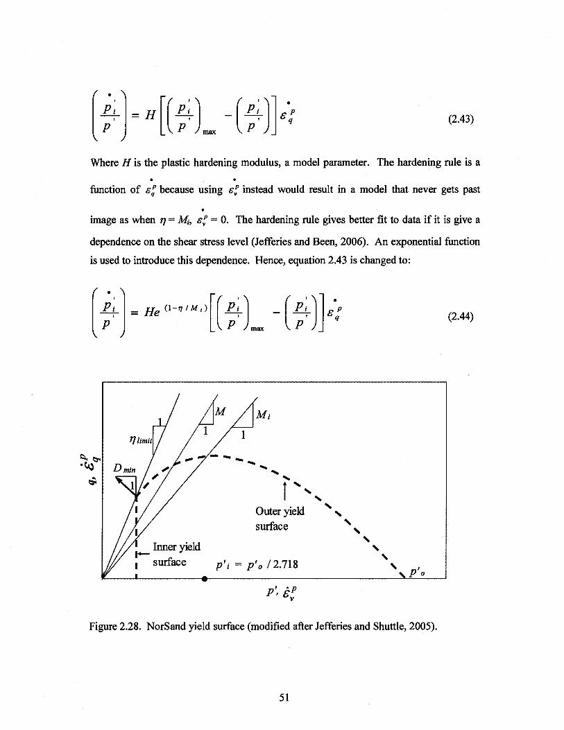
.
= H [(J -
(2.43)max
Where H is the plastic hardening modulus, a model parameter. The hardening rule is a
function of 8’ because using s’ instead would result in a model that never gets past
image as when i = M,, s = 0. The hardening rule gives better fit to data if it is give a
dependence on the shear stress level (Jefferies and Been, 2006). An exponential function
is used to introduce this dependence. Hence, equation 2.43 is changed to:
[] = He(1/Mi)[Jmax
- (2.44)
Figure 2.28. NorSand yield surface (modified after Jefferies and Shuttle, 2005).
51

0
.:.a
a_
Data from 13 sands • a:ii
-0.2 a
I
I a 1 a
a Ia —a a
a — aI
.4- II —a a •a a
ag ao6 a a a a
a: a —— a
a a-0.8
— 1
-0.3 -0.2 -0.1 0
State parameter at image,
Figure 2.29. Minimum dilatancy as a function of state parameter at image for 13 sands(modified after Jefferies and Been, 2006).
2.5.3. Typical evolution of the yield surface
The hardening and softening ofNorSand yield surface is described as follow (see
Jefferies 1993):
• It is assumed that we are starting with a soil denser than the critical state.
• With increasing shear strain the yield surface hardens, with the size of the
yield surface during hardening controlled by the mean effective stress at
image, p’s. Soil remains contractive until the current mean effective stress
equals p,.
• Although the current stress ratio is equal to M, the movement of the yield
surface does not stop because the image state only satisfies one condition of
the critical state. The hardening continues with increasing shear strain in a
52

dilative manner until it reaches the surface corresponding to the limiting stress
and maximum allowable dilation rate.
• At this point, softening starts with a decreasing rate as it approaches the
critical state.
• At the critical state M = M and the yield surface does not move any further.
2.5.4. Elastic properties of NorSand
In Cam-Clay elasticity, the elastic shear strains are ignored. NorSand does not ignore
the elastic part of shear strains and variations on elasticity including standard linear
elasticity and a range of stress dependent models have been implemented.
2.5.5. Summary of the NorSand model
The full set of equations that specify the NorSand model presented in the preceding
sections are given in Table 2.1. Table 2.2 lists the parameters used in the model and their
typical ranges. The parameter ranges were primarily obtained from calibrations to sand,
so care should be exercised when applying to other soil types.
53

Table 2.1. Summary ofNorSand equations (modified after Jefferies and Shuttle, 2005).
Aspect of NorSand Equation
Internal model parameters ,p- = e—
e =F—2eln(p’) and,
M. =M-x411
Yield surface
1—
with I -E--l = e ‘ I M1)LL =
M1 PI} L1’ Jmax
Flowrule D’9 =M1—
Hardening of outer yield (surface = He (1/M1)E(J’
—
[ Pjmax
Elasticity = G /p
54

Table 2.2. Summary ofNorSand parameters (after Jefferies and Shuttle, 2005).
Parameter I Typical range DescriptionCritical stateF 0.9-1.4 The y-intercept of the e
log(p curve at 1KPa2e 0.01 — 0.07 The slope of CSL in e
log(p’) space defined onbase e
JvI 1.2-1.5 q/p’at critical statePlasticityH 50-500 Plastic hardening modulus%tc 2.5-4.5 A parameter that limits the
hardening of the yieldsurface
N 0.2-0.4 The volumetric couplingparameter (used in Nova’srule)
ElasticityJr 100-800 Dimensionless shear rigidity
(G/pv 0.1-0.3 Poisson’s ratio
2.6. Soil behaviour in unloading
While there have been relatively many studies addressing the overall cyclic behaviour
of sand, little work has been done to study the behaviour of sand during the unloading
phase in detail. It is interesting that sand also shows contractive, in addition to the
expected dilative, behaviour when unloaded. The implications of this behaviour were
discussed in Chapter 1. This section discusses previous work on the topic.
2.6.1. A Simple physical model
Jefferies (1997) explains soil contraction in unloading in terms of stored potential
energy during the loading phase. Assuming the saw tooth model represents how soil
dilates, when dense sand is loaded grains tend to climb over the slip surfaces (see Figure
55

2.30a). This is associated with increase in volume as the voids between the teeth are
increased. At the end of loading the potential energy of those particles has been
increased by the virtue of their new location. When unloading, it is then easy to imagine
that those particles will tend to slide backwards (see Figure 2.30b). This is associated
with decrease in volume as the voids between the saw teeth get smaller (d2 < d1).
2.6.2. Thermo-mechanical approach
The first law of thermodynamics states that “The increase in the internal energy of a
system is equal to the amount of energy added by heating the system, minus the amount
lost as a result of the work done by the system on its surroundings”. Alternatively, plastic
work done on soil is either dissipated in the form of frictional energy or contributes to the
increase of internal energy.
Cam-Clay assumes that all ‘plastic’ work done on soil is dissipated. This means that
plastic work does not contribute to changing internal energy. Part of the total work
increments is recoverable (termed ‘elastic’) and the other part is irrecoverable (termed
(a)
(b)
Id1
Id2
‘I
Figure 2.30. The Saw Tooth Model a) loading phase b) unloading phase.
d1>d2
56

‘plastic’) as in Equation 2.45. Cam-Clay is rigid in ‘elastic’ shear and only recovers
‘elastic’ volumetric strain. Therefore, the Cam-Clay approach assumes that any change
in internal energy is only due to an ‘elastic’ change of volumetric strain that can be
calculated using the slope of the swelling line in a usual consolidation test (Schofield and
Wroth, 1968). The ‘plastic’ component of work is dissipated and the dissipation rate is
assumed constant and equal to the critical friction ratio, M. The term on the right hand
side of Equation 2.45 represents plastic work dissipation and cannot be negative (as all
work dissipation is positive). Dividing Equation 2.45 through by ./i6q’ and rearranging
yields the Cam-Clay flow rule, Equation 2.46.
(2.45)
Where,
is the ‘plastic’ work (unrecoverable according to Cam-Clay) done per unit volume
is the total work done per unit volume
is the ‘elastic’ work (or recoverable) per unit volume
(2.46)
However, the Cam-Clay flow rule does not fit sand data as well as Nova’s rule in
Equation 2.47. Nova (1982) derived his flow rule based on experimental observations.
Dp=M7 (2.47)1-N
Upon substituting for D” and ,j and rearranging,
57

+ p’ = Mp + Np’ (2.48)
If soils were not to violate the first law of thermodynamics, then work done on the soil
sample is either dissipated or contributes to a change in the internal energy of the sample.
The two terms on the right hand side of Equation 2.48 represent plastic work done. The
first term on the right hand side represents the dissipation mechanism as discussed earlier
in this section. It is then reasonable to assume that the second term on the right hand side
contributes to a change in internal energy. In other words it represents a stored energy.
Jefferies (1997),calls it ‘plastic’ stored energy. It is not elastic as it is not reasonable to
assume that plastic work done on the sample is transferred into stored elastic energy. It is
stored energy, i.e. not dissipated, because the term can take negative sign.
Cam-Clay assumes that all plastic work dissipation is represented by the first term on
the right hand side. Based on this assumption, any other term on the right hand side
represents something other than dissipation of plastic work. Therefore, according to
thermodynamics, it represents changed internal energy or stored ‘plastic’ energy.
The idea of a change in internal energy due to change in plastic strains was first
proposed by Palmer (1967). Palmer’s approach is illustrated in Figure 2.31.
Total Work Done
[ Dissipated frictional energy Change in internal energy
L f() J L______________________r
I\ r
I
Due to change in Due to change in ‘ (term
1 (rigid in elastic shear) J L ignored in Original Cam-Clay)
Figure 2.31. Energy balance as introduced by palmer (1967).
58

To justify this, Palmer (1967) considers a hypothetical experiment where the state of
soil moves along the critical state line in the e-p’ space. While moving along the CSL
shear deformations -in this case all deformations are plastic as Palmer’s model as well as
Original Cam-Clay are rigid in elastic shear- resisted by friction are not expected to
contribute to any change in volumetric strain and the Original Cam-Clay energy balance
equation reduces to:
= (2.49)
But because we are hypothetically moving on the CSL, and different pressures are
associated with different critical void ratios, then there must be a change in volumetric
strain. Most of this change is ‘plastic’ because the CSL is usually much steeper than the
swelling lines. However, Equation 2.49 fails to predict this change. Therefore, another
term should be added to represent changes in internal energy due to change in plastic
volumetric strain. This term turns out to be the ‘N’ term on the right hand side of
Equation 2.48.
Jefferies (1997) assumes that all the stored ‘plastic’ energy is recovered upon
unloading. Solving Equation 2.48 for the case of unloading while changing the sign of
the ‘N’ term, as it is energy recovered in unloading, gives the following:
q8’+p8’ ——Mps’—Np6,’ (2.50)
Upon rearranging and substituting,
Dp=M (2.51)1+N
Equations 2.46, 2.47 and 2.51 are plotted in Figure 2.32. It will be shown later that
triaxial laboratory data shows a different trend for stress-dilatancy in unloading from that
represented by Equation 2.51.
59

Stress-dilatancy in unloading\according to Jefferies (1997); \ 0.4
D’1 =(-M- )i(1+N) forM =
1.27andN=0.4
-3 -2 -1
D
Figure 2.32. Stress-dilatancy for Cam-Clay loading, Nova loading, and Jefferies (1997)unloading.
Collins (2005) discusses a different conceptual model for yield in unloading from a
thermo-mechanical viewpoint, taking into consideration differences between the micro
scale where the particles interact, and the continuum scale where most soil constitutive
models are defined. The model is summarized in Figure 2.33. The difference between
Collins (2005) approach and that of Palmer (1967) and Jefferies (1997) is that the former
assumes that stored elastic energy is the cause for yield in unloading while this is not the
case for the latter. Collins model is illustrated in the following paragraph.
Pure hydrostatic loading on the continuum scale is assumed and following the usual
convention the applied work may be separated into an elastic and plastic component.
During loading part of the applied work is dissipated while the remainder is stored in
terms of elastic compression of soil particles. In subsequent unloading, part of the stored
elastic work is released causing dilation while the other part can only be released if
Nova’s rule (M =
1.27 andN = 0.4)
0.8
0 1 2
60

associated with particle rearrangement. Particle rearrangement is not elastic and hence
plasticity occurs during unloading. Hence it is implied that all plastic strains during
unloading are dilative. It is assumed that most of the total shear energy is dissipated as
plastic work.
Total work done in loading
Hydrostatic compressioncomponent
Shear component
Figure 2.33. Schematic representation of work storage and dissipation according toCollins (2005).
Stored (elasticcompression ofparticles on themicro scale)
Dissipated(plastic particlerearrangement)
Most of the total shearenergy is dissipated asplastic work
Upon unloading, part of stored elasticenergy is recovered (elastic expansionwith no particles rearrangement)
Stored elastic shear energy(Very little contribution tofrozen energy)
Upon unloading, some of the storedelastic energy cannot be recoveredwithout particle rearrangement. Theenergy associated with particlerearrangement is termed ‘frozen energy’and is dissipated as plastic dilationduring unloading.
61

2.6.3. Unloading in NorSand
Jefferies (1997) presented a framework for the NorSand model in unloading and
subsequent reloading. Because this model is extended as part of the current work, a more
detailed discussion of the Jefferies (1997) unloading model is provided in this section.
The NorSand model was described in Section 2.5 with emphasis on monotonic loading
conditions. This section discusses in more details the unload-reload version ofNorSand.
In unloading, soil yields at the inner cap. The inner yield surface (or inner cap) is the
vertical part of the yield surface shown in Figure 2.28. Its location at the outer yield
surface is chosen to fit within the framework of the NorSand model in loading and is a
vertical straight line for simplicity. This internal cap scales with the outer yield surface
and is located at:
Peap = e(_1)mjM1)(2.52)
The NorSand flow rule in unloading was derived earlier in Section 2.6.2 as Equation
2.51. Jefferies (1997) introduced a rule to govern the movement of the inner cap, i.e. a
hardening rule, as:
1
___
8v “lflI I (2.53)Hp %P)
Where,
H is the hardening (softening) modulus in unloading
pji is the mean effective stress at first yield in unloading (i.e. the mean stress of the cap
when first intersected)
62

So far the model definition is completed. The rest of this section presents two
examples of stress paths (Figure 2.34 and Figure 2.35) to illustrate the model behaviour.
Figure 2.34 shows a stress-strain curve with a single unload-reload loop and the yield
surfaces corresponding to the load-unload-reload phases. The points of interest are
annotated on the stress-strain curve, i.e. the plot at the left top side, and on the yield
surfaces corresponding to loading, unloading and reloading, i.e. plots on the right top, left
bottom, right bottom sides respectively. The darker lines represent the surface where
current yield is occurring. The thicker lines represent the stress path. The yield surface
hardens with loading until the internal cap is reached as in Figure 2.34, i.e. path 1-2.
Point 2 in the figure represents peak strength and is associated with the maximum size of
the yield surface. With continued shearing further strain causes softening and the stress
path softens to reach point 3.
Another stress path is illustrated in Figure 2.35 which has a similar arrangement as for
Figure 2.34. Unloading in this case occurs from a point before reaching the internal cap
that represents peak conditions. Loading causes hardening of the yield surface along path
1-2. The internal cap scales with the yield surface.
In unloading, there are three possible cases for the stress point to move on or inside the
yield surface:
Case 1:
The stress point touches the internal cap in loading, unloading then cause plastic
softening of the yield surface. This is illustrated in Figure 2.34 where yielding
occurs as the stress point moves on the internal cap from point 3 to point 4. As
the cap moves with the stress point, the outer yield surface also softens.
Case 2:
The stress point does not touch the internal cap in loading, as shown in Figure
2.35. Upon unloading, the yield surface does not move until the stress point
touches the internal cap. Before this point, unloading is purely elastic (Figure
63

2.35). After the stress point touches the cap yielding starts on the cap and the
yield surfaces soften until the stress point reaches location 3.
Case 3:
The third case occurs for unloading early in the stress path. Under these
circumstances the stress point does not touch the cap during unloading and the
whole unloading phase remains elastiö.
Under all situations reloading is elastic as long as the stress point is inside the outer
yield surface (see Figure 2.34 and Figure 2.35). Once the stress point touches the outer
yield surface, plastic reloading continues as in the virgin loading phase.
S -
Loading
where
0 200 200 200 400 000 660 00
1.20
120
0.00
0.40
2
Sreface where cuffent yield
1
• Cununtotresopoint
100
0 5 10 15 20 25
er:%
200 -
3
,.-‘Unloading
200 /,‘,
surfaces where
\,N
200
100
0
5
___________________
Reloading
Surla swherecurrent y Id is
I. 0 urnng
£Ittsti.relooding
p.
100 200 300 400 600 600 0 10 200 300 400 000 600 700
Figure 2.34. Movement of yield surface in NorSand: Case of unloading from a point onthe internal cap.
p.
64

1.80 2
200Loading
° 2 Surface where cusT006 yield /7 /::
_____________________________________
I:
\pcciJmng
0 5 16 65 20 0 570 200 300 400 600 800 700
300 300 4
200/ V} Unloading
230 A! Reloading
/ Suaces ere . It S ces ere
‘:
current yId is
:
ttcre1oad\\’”\
0 100 200 300 400 570 800 700 0 100 200 300 400 500 600 700
p p’
Figure 2.35 Movement of yield surface in NorSand: Case of unloading from a point
before reaching the internal cap.
2.6.4. Summary
It can be seen from this selective review of soil behaviour in unloading that soil
behaviour in unloading is still not well understOod. There is no agreement on the cause
of yield in unloading, for example the Jefferies model implies that it is mainly caused by
plastic shear deformation in loading while Collins attributes yield in unloading to
rearrangement caused by elastic dilation of particles associated with reduction in mean
effective stress. Clearly, this topic needs more investigation as it is important for
earthquake engineering. A practical model that accounts for yield in unloading is
required. Understanding stress-dilatancy in unloading is one of the requirements of such
a model and is discussed in the following chapter.
65

3. DILATANCY IN UNLOAD-RELOAD LOOPS: A THEORETICAL
INVESTIGATION
Dilatancy in loading has been investigated by many researchers as discussed in Section
2.4. Most elasto-plastic constitutive models have yield surfaces that were developed for
stress paths involving increasing shear; a reduction of shear stress (i.e. unloading) within
that surface is considered elastic. But contraction has been observed during unloading for
the standard triaxial stress path. Standard elasticity would predict expansion during
unloading. Hence, these observations suggest that the soil is yielding during unloading.
Constitutive models that incorporate yield in unloading are rare. The topic is not well
covered and is controversial as shown in Section 2.6. The objective of this chapter is to
develop theoretical understanding of dilatancy in unloading as well as in subsequent
reloading phases. The investigation is done at the micro-mechanical level.
3.1. Micro-Mechanical perspective for dilatancy in unloading
The standard elasto-plastic approach assumes that soil is a continuum. However, in
reality, soil is composed of discrete particles and plasticity is an abstraction used to
explain what really happens between the grains. It is of interest to develop an
understanding of why soil contracts in unloading from a microscopic point of view.
Rowe (1962) derived an expression for dilatancy in loading based on frictional forces
between rigid cylindrical rods (see Section 2.4). Rowe assumed identical rods that are
rigid and have a circular cross-section. The forces at the contacts are assumed purely
frictional and the initial packing does not change during shearing. Packing represents the
pattern at which particles are arranged relative to each other. For example, Figure 3.1
shows one possible packing for the rods but three different particle assemblies. The three
66

different particle assemblies in the middle of Figures 3.1 a,b, and c have the same
packing. The relative arrangement of particles in the three assemblies does not change,
i.e. if particle ‘x’ happens to be to the right of particle ‘y’ in the first assembly, then it
stays to the right ofparticle ‘y’ in the other two assemblies.
A change in the volume of the packing can be explained by taking four particles aside.
In loading, as illustrated using the four particles on the left hand side of Figure 3.1, if the
upper grain is pushed vertically downward the two side grains will move outwards. This
will be associated with an increase in volume if the angle between the tangent to grains
interface and the vertical direction, f3 > 45° (see Figure 3.la). However, for f3 < 45° when
the upper particle is pushed down the assembly decreases in volume (see Figure 3.1 c).
By computing the work done by the major principal stress on the assembly to the work
done by the assembly on the minor principal stress for rigid rods, Rowe derived the
following equation (the complete derivation is given in Section 2.4):
= tan(qS + ,6)(3 1)
2 ; (1+ ) tan fi
Where,
a’j is the major principal effective stress
a’2 is the minor principal effective stress
is the rate of change in major principal strain
2 is the rate of change in minor principal strain
is the rate of unit volume change
q5 is grain to grain friction angle
fi is the angle between the tangent to grains interface and the vertical direction
And for the packing in Figure 3.1,
67

= tan(/1) tan(q5 + /3) (3.2)
C)
I2 4,
8 12
Figure 3.1 Micro-mechanical representation of dilatancy for a uniform packing of rigidrods during both loading and unloading a) Minimum void ratio for ft = 600 b) Maximumvoid ratio forfi = 450 c) Minimum void ratio forfi = 30°
LOADING a
I2 4,a)
32’ 24-
b)
UNLOADING
I2 f
82! 2-
12 t
W112 4,
I 2
oI 24-
62124-
a2
o1I2
o12
82! 2-
Equation 3.1 is valid for different packings of rigid rods but the stress ratio in Equation
3.2 depends on the packing type (i.e. the pattern at which particles are arranged relative to
each other). For the packing in Figure 3.1, Rowe showed that stresses and strains in
68

direction 1 over those in direction 2 can be expressed as in Equations 3.2 and 3.3,
respectively.
1(3.3)
82tan2 /3
Multiplying Equation 3.2 by 3.3 yields equation 3.1. Note that Equations 3.2 and 3.3 are
identical to Equations 2.20 and 2.21 for a = /3, which is the case for this packing.
For the packing on the right hand side of Figure 3.2 Li and Dafalias (2000) showed,
following a similar derivation as for Equations 2.20 and 2.21 in Section 2.4, that
Equations 3.4 and 3.5 below should be used instead of equations 3.2 and 3.3,
respectively. The reason for having different equations is that the volume of the basic
unit defined by the dashed rectangle in Figure 3.2 for each of the packings is different.
The complete derivation is given in Li and Dafalias (2000).
--=tan(q5,2sin/5
(34)1+2cos/1
—— (1+2 cos /3) cos /3 (3 562
2sin2fl)
Note that multiplying Equation 3.4 by 3.5 also yields Equation 3.1. Therefore, Equation
3.1 is valid for different packings, while the ratio between stress in direction 1 to that in
direction 2 is packing specific. Therefore, if the term 6v18i in Equation 3.1 is assumed
to represent dilatancy, then there are different stress-dilatancy relations for different
packings.
69

Unloading can be explained in the physical sense by reference to the illustrations on the
right hand side of Figure 3.1. If the side grains are pushed inwards, the upper and lower
grains will move outwards. This is associated with decrease of volume iffi> 450•
As discussed above, Equation 3.1 is derived for loading based on an energy balance
between the ratio of work done by a strain increment in direction 1 on the assembly to
that done by the assembly in direction 2. Part of work done in the form of a strain
increment on direction 1 is dissipated in the assembly by friction while the remaining
work is transferred to direction 2.
Assuming that soil is an isotropic material and the packing does not change during the
loading and unloading phases, work balance in unloading can be thought of as the ratio
between the work done by a strain increment in direction 2 on the assembly to that done
by the assembly on direction 1. In other words, the proposed expression for dilatancy in
unloading based on grain to grain friction is the same as the usual one of Rowe (1962)
but with the assembly rotated by 900, i.e.:
8i = = tan(q5M +90—(3 6)
U;62 J;(1+6v/6i)tan(90-fi)
= tan(90— fi) tan(q + 90— ,6) (3.7)
Figure 3.3a plots the proposed relation for dilatancy for unloading, i.e. Equations 3.6
and 3.7, as compared to that for loading. fi for unloading is equal to 90°-fl of that for
loading, as a consequence of rotating the assembly (Figure 3.3b). Note that Equation 3.7
is only valid for the packing in Figure 3.1.
Erksak 330/0.7 sand is a quartz sand with an average grain size of 330.tm. The grain to
grain friction angle, q, can be estimated for quartz as 25° (Rowe, 1962). Figure 3.3a
70

shows a comparison between the dilatancies for the loading phase and first unloading for
a drained triaxial test on Erksak sand (p’ = 100 kPa and e0 = 0.653) to the theoretical
expressions based on grain to grain friction for q = 25°. The fit is a very good one for
both loading and unloading considering the previously stated assumptions involved in
deriving the theoretical expression. However, it is not as good for the reloading phase
and the second unloading ioop (not shown in the figure). This is to be expected as soil
fabric changes with continued shearing, while the theoretical expression is only valid for
the packing in Figure 3.1.
Packing A Packing B
Figure 3.2. Two different uniform assemblies of rigid rods; the dashed rectanglerepresents the basic unit volume (reproduced after Li and Dafalias, 2000).
3.2. Micro-Mechanical perspective for dilatancy in reloading
The stress-dilatancy relation is expected to change for different reloading phases. The
reason is due to particle arrangement (i.e. fabric) changes during shearing. Let us assume
that we have two different uniform packings of rigid cylindrical rods similar to those in
Figure 3.2. Packing B has a higher void ratio than packing A. For the sake of the
argument, it is assumed that during an unload-reload phase the arrangement of the rods
changes from a packing similar to B to another one similar to A. This change can be
71

thought of as being equivalent to change in fabric in real soils. As discussed in Section
3.1, the stress-dilatancy relation is different for the two packings. Equation 3.1 is valid
for the two packings. However, the stress ratio (i.e. oil a2) is different for packing A
and B as in Equations 3.2 and 3.4, respectively. The stress ratio in unloading for packing
A is as in Equation 3.7. Similarly, the equation for stress ratio in unloading for packing B
is:
-1-=tan(b +90—fl)2sin(90—fl)
(3.8)M 1+2sin(90—fl)
Equations 3.1, 3.2, and 3.4 were used to plot the loading curves in Figure 3.4.
Equations 3.6, 3.7 and 3.8 were used to plot the unloading curves. The predicted stress
ratio for a given dilatancy is lower for the denser packing as expected. The trend from
triaxial laboratory data agrees with the trends in Figure 3.4 as will be shown in the next
chapter.
Rowe (1962) recognized that particle relocation occurs with shearing, and as a result
the value of/I changes in a non-uniform manner because real soil particles are not of the
same size and shape. He assumed that this relocation would happen in a way such that
changes in the values of/I would keep the rate of internal work done to a minimum. This
assumption changes Equation 3.1 to Equation 3.9 which is independent of fi and therefore
independent of packing and density (the complete version of Rowe’s derivation is given
in Section 2.4). The assumption of minimum internal work predicts a single stress
dilatancy relation to be valid for all packings. Li and Dafalias (2000) disagree with
Rowe’s use of the assumption of minimum internal work and therefore they predict that
the stress-dilatancy relation is different for different packings. Rowe’s stress-dilatancy,
Equation 3.9, is an idealization that is applicable for a random mass of irregular soil
particles. It contradicts the exact solution, i.e. Equations 3.1-3.8, that clearly shows that
stress-dilatancy is dependent on packing.
72

a)
-056v/81
Figure 3.3 Theoretical expression based on grain to grain friction (q=25°) for theuniform packing in Figure 3.1 a) compared with a drained triaxial test on Erksak 330/0.7(p’= 100 kPa and e0 = 0.653) in stress ratio vs. dilatancy space, b) Angle between thevertical direction and the tangent at the interface between grains.
U; (1+ d V/V)= tan2(45+O.Sç!i) (3.9)
Overall, this section showed that the stress-dilatancy relation is dependent on packing.
For example, packings A and B in Figure 3.2 have different stress-dilatancy relations as
C,
b)-1 -0.5 • 0
8 / s i
on
0.5
‘Jy
Loading55
50
35
. 30—1 0 0.5
73

shown in Figure 3.4. As the packing is expected to change in a reloading phase
compared to that for first loading, a change in stress-dilatancy is expected in reloading.
3.3. Summary
The study of two packings of rigid rods showed that yield in unloading occurs. In this
chapter, a stress-dilatancy relation in unloading was derived based on a micro-mechanical
approach. The derived relation turns out to be identical to Rowe’s stress-dilatancy in
loading while rotating the packing of rods by 900. The study of deformation
characteristics in reloading using a micromechanical approach showed that stress
dilatancy changes in reloading compared to first loading. Reloading is associated with a
more dilative response than first loading.
0
0.5
Figure 3.4. Rowe’s stress-dilatancy relation based on grain to grain friction for the twopackings in Figure 3.2
-1 -0.5 • 08 vi 6 1
74

4. DILATANCY IN UNLOAD-RELOAD Loops: AN EXPERIMENTAL
INVESTIGATION
The previous chapter addressed dilatancy in unloading and reloading from a micro-
mechanical point of view. In order to compare the trends predicted from the micro-
mechanical approach to the trends observed in real soils, and to apply these observed
trends to a general continuum model for future application to liquefaction modelling, this
chapter investigates observed stress-dilatancy for two sands in drained triaxial tests that
include unloading and reloading cycles.
4.1. Sands Tested
Erksak sand (ES) and Fraser River sand (FRS) were used in this study. ES was chosen
because drained triaxial tests with load-unload-reload cycles were available (Golder
Associates, 1987; www.golder.com/liq). Note that the focus of this chapter is to
investigate stress-dilatancy and therefore drained tests were used. FRS was chosen
because of the availability of new monotonic triaxial tests and drained load-unload-reload
triaxial tests undertaken by Golder Associates.
4.1.1. Erksak Sand
Erksak sand, a sand that was used in the construction of the Molikpak core in the
Canadian Arctic, is a uniformly graded medium-grain sub-rounded sand, mainly
composed of Quartz and Feldspar. The gradation of Erksak sand used, Erksak 330/0.7,
had an average particles size of 330 jim and fines content of 0.7%. The Index properties
are presented in Table 4.1. Its specific gravity is 2.66. The index density measures, emin
75

and emax, according to ASTM test methods D4253-00 and D4254-00 are 0.525 and 0.775,
respectively (ASTM 2006a; ASTM 2006b; after Sasitharan, 1989).
4.1.2. Fraser River Sand
Fraser River sand originates from the alluvial deposits of Fraser River located in British
Columbia, Canada. It is a uniformly graded medium-grain sand with angular to sub-
rounded particles. It is mainly composed of Quartz, Feldspar and unaltered rock
fragments with an average particles size of 260 im (see Table 4.1). Its specific gravity,
emin, and emax are 2.75, 0.62, and 0.94, respectively.
Table 4.1: Index properties of Fraser River and Erksak sands
Fraser River sand, Erksak sand,Sriskandakumar (2004) Been et al. (1991)and Chillariage et. al. and Sasitharan(1997) (1989)
Mineralogy 40% Quartz, 11% 73% Quartz, 22%feldspar, 45% Feldspar, and 5%unaltered rock other mineralsfragments and 4% ofother minerals
Median grain size D50: pm 260 330Effective grain size D10: pm 170 190Uniformity coefficient 1.6 1.8Percentage passing no. 200 0 0 7sieveSpecific gravity of particle 2.75 2.66Grain description Angular to sub- Sub-rounded
roundedMaximum voids ratio em 0.94 0.775Minimum voids ratio emin 0.62 0.527
76

4.2. Testing program
All tests reported in this section are conventional triaxial compression tests (i.e.
confining stress is kept constant during the shearing phase). The testing procedure and
sample preparation methods are described in Appendix E.
The full Erksak testing program included 29 drained and 39 undrained triaxial tests. As
this investigation focuses on volumetric changes drained tests were of primary interest,
although five of the undrained tests on ES were used to better define the location of the
critical state line (see Chapter 6). Of the available drained triaxial tests, the ten drained
tests that followed a conventional triaxial stress path, and also contained load-unload-
reload cycles, were used for this work. The data for all of the Erksak tests are available
for download from the web site: www.golder.com/liq.
The FRS testing program included 6 drained and 2 undrained triaxial tests. Six
monotonic tests on FRS, 4 drained and 2 undrained, are used for the monotonic
calibration of NorSand to FRS (see Chapter 6). The two drained unload-reload tests on
FRS are used to validate the predictions of the calibrated unload-reload model in Chapter
7.
4.2.1. Erksak Sand Testing Program
The ES load-unload-reload tests are summarized in Table 4.2. The ten tests cover a
wide range of mean effective stresses (100-800 kPa). The range of void ratios is 0.603-
0.723. All of the samples were water pluviated except for ES_CID_868 that was moist
tamped. These ten tests were performed under drained conditions to enable review of the
volumetric change characteristics of sand. The number of unload-reload loops in the tests
varies between one and three. In some tests the unload-reload loops occur before
reaching peak strength, while other unload-reload loops are post-peak. This allows the
77

investigation of stress-dilatancy during unloading and reloading at different strain and
stress levels.
The ES undrained monotonic triaxial testing used to determine the critical state line is
summarized in Table 4.3. All of the moist tamped tests are on loose samples with void
ratios close to emax. Undrained conditions and loose samples were chosen so that the
samples can reach critical state within the limitation of the apparatus.
Table 4.2: Drained triaxial compression tests on Erksak Sand with load-unload-reloadcycles (data from www.golder.com/liq)
P’ e0 Preparation Number ofTest No. (kPa) method’ U-R loops2
ES_CID_860 100 0.672 WP 1ES_CID_861 100 0.645 WP 2ES CID_862 100 0.645 WP 3ES_CID_866 400 0.698 WP 2ES_CID_867 400 0.680 WP 3ES_CID_868 400 0.723 MT 2ES_CID_870 800 0.653 WP 1ES_CID_871 800 0.637 WP 2ES_CID_872 800 0.652 WP 3ES CID_873 100 0.603 WP 3
‘WP stands for water pluviated and MT stands for moist tamped.2U-R stands for unload-reload
Table 4.3: Undrained monotonic triaxial compression tests on Erksak sand (data fromBeenet.al., 1991)
1MT stands for moist tamped.
p’ e0 PreparationTest No. (kPa) method1
ES_L_601 499 0.754 MTES L_604 699 0.768 MTES_L_605 500 0.766 MTES_L_606 701 0.759 MTES L607 701 0.748 MT
78

4.2.2. Fraser River Sand
Table 4.4 presents the test conditions of two load-unload-reload tests undertaken
recently by Golder Associates on FRS. Both samples were moist tamped. The confining
pressure for each test is similar at 190 kPa and 198 kPa, but the corresponding void ratios
differ, being 0.89 and 0.72 respectively. Both tests had more unload-reload loops than
the ES tests (four and five loops, while the maximum number of loops for ES was three).
Four drained and two undrained monotonic triaxial compression tests on moist tamped
samples were carried out (see Table 4.5 for a summary of the test details). The undrained
tests were used to obtain critical state parameters, while the drained tests were used for
the FRS monotonic calibration to the NorSand model. The consolidation stresses ranged
from 50 kPa to 515 kPa ande0ranged from 0.63 to 0.91.
Table 4.4: Drained triaxial compression tests with load-unload-reload cycles on FraserRiver sand (data provided by Golder Associates)
p’ (kPa) e0 Preparation Number ofTest No. method’ UIR loops
FR_CID 01 190 0.89 MT 5FR_CID_02 198 0.72 MT 4
1MT stands for moist tamped.2UR stands for unload-reload.
79

P’ (kPa) PreparationTest No. e0 Test type method1FRCID 03 114 0.67 Drained MTFR_CID_04 410 0.63 Drained MTFR CID 05 515 0.69 Drained MTFR_CID_06 50 0.75 Drained MTFR_CU_01 388 0.91 Undrained MTFR_CU 02 196 0.82 Undrained MT
‘MT stands for moist tamped.
4.3. Experimental observations
The main focus of the review of experimental results was stress-dilatancy in unloading
and subsequent reloading. To the knowledge of the author, an experimental review to
specifically investigate stress-dilatancy trends in unloading has not been done before.
The issue of concern .is what factors determine whether soil is likely to contract or dilate
in unloading and the amount of those volumetric changes. The effect of the loops on
peak strength and volumetric changes in reloading is also investigated.
In the following discussion “U” refers to an unloading loop and “L” refers to a loading
or reloading loop. The number following the symbol denotes the order of a particular
loop from the beginning of the test.
A typical test on Erksak Sand is plotted in Figure 4.1. The strength of the sand, shown
in Figure 4.la, does not seem to be highly affected by the unload-reload loops. The data
shows that loop U 1 does not introduce a local peak in the stress-strain curve. However,
loops U2 and U3 show small peaks slightly affecting the stress-strain curve. Loop U 1
occurs before the image state which marks the boundary between contractive and dilative
behaviour as annotated in Figure 4. lb. Loop Ui is not followed by a small peak and the
stress strain curve seems to continue as if the unload-reload loop did not exist. However,
loops U2 and U3, post-image loops, are followed by small peaks. The peaks on reloading
Table 4.5. Monotonic triaxial compression tests on Fraser River sand (data provided byGolder Associates)
80

appear larger in Figure 4.2 which plots shear stress vs. axial strain (rather than the stress
ratio vs. axial strain plotted in Figure 4.1 a). The other tests on Erksak sand (see
Appendix B) and Fraser River sand (Figure 4.3) demonstrate similar behaviour.
Conversely, volumetric strains are dramatically influenced by the unload-reload loops.
Both the absolute values and the rates of change are affected (Figure 4.lb). Unloading
occurs starting from pre-image conditions for Ui. Note that volumetric changes
associated with unloading are very small and are initially contractive followed by a small
dilative phase (see Figure 4.4 for a zoom on loop 1). However, for U2 and U3,
volumetric changes associated with unloading are significant. They are dominantly
contractive (see Figure 4.4 for a zoom on loop 2). Note that unloading for those two
loops starts from post-image conditions.
Table 4.6 summarizes the direction of volumetric changes in unloading for the load-
unload-reload tests on ES. The information provided includes the stress ratio and axial
strain at image stage. For each unload-reload (U-R) loop the stress ratio at which
unloading starts is given, together with the axial strain, whether the ioop starts pre or post
image, and whether the volumetric strains are dilative or contractive. It can be observed
that whenever unloading happens from post-image conditions, volumetric strains are
either totally contractive or dominated by contraction. Conversely, if unloading occurs
from pre-image conditions, volumetric strains are either totally dilative or dominated by
dilation.
Table 4.6. Direction of volumetric changes in unloading for the load-unload-reload testsonES
Test U-R loop’ Stress ratio Axial Pre/Post Dilative/Contractive
Strain (%) image during unloading
ES_CID_860 Image 1.114 0.402 At -
1 1.419 10.073 Post Con.
ES_CID_861 Image 1.098 0.544 At -
1 1.362 1.778 Post Mostly con.
2 1.484 10.014 Post Con.
81

Test U-R loop’ Stress ratio Axial Pre/Post Dilative/Contractive
Strain (%) image during unloading
ES_CID_862 Image 1.163 0.667 At -
1 0.353 0.9 Pre Dil.
2 1.377 1.768 Post Mostly con.
3 1.481 10.122 Post Con.
ES_CID_866 Image 1.169 2.644 At -
1 1.265 4.50 1 Post Mostly con.
2 1.359 10.064 Post Mostly con.
ES_CID_867 Image 1.107 1.082 At -
1 1.102 1.033 Pre Mostly dil.
2 1.338 4.05 1 Post Mostly con.
3 1.393 10.101 Post Con.
ES_CID_868 Image 1.209 3.68 At -
1 1.2 12 4.047 Post Mostly con.
2 1.269 10.146 Post Con.
ES_CID_870 Image 1.177 1.807 At -
1 1.352 10.056 Post Mostly con.
ES_CID_871 Image 1.16 1.84 At -
1 1.308 4.035 Post Mostly con.
2 1.366 10.108 Post Mostly con.
ES_CID_872 Image 1.209 1.814 At -
1 1 1.022 Pre Dil.
2 1.348 4.0 18 Post Mostly con.
3 1.405 10.107 Post Con.
ES_CID_873 Image 1.194 0.3 19 At -
1 1.079 0.234 Pre Dii.
2 1.5 13 1.53 1 Post Mostly con.
3 1.5 10.073 Post Con.
Image indicates the stressbehaviour in loading)
ratio at image (image marks the boundary between contractive and dilative
82

Figure 4.1 c presents the data from the same example ES test used previously, test
ES CID 867, in stress-dilatancy space. The following equation was used for calculating
dilatancy from laboratory data:
D8(+i) 8(—i) (4.1)6q(n+1) 6q(n—1)
where 11 denotes the current step.
In the case of unloading, positive dilatancy means volume increase while negative
dilatancy indicates volume decrease. For unload phases U2 and U3 in Figure 4.lc, the
sample contracts in unloading except for one point in U2. Unloading for those two
phases starts from post-image stress ratios. Conversely, for Ui where the sample is
unloaded from a pre-image stress ratio, the sample increases in volume at the beginning
of the unloading phase. Then the sample contracts towards the end of the unloading
phase. This behaviour shows that soil does not unload in an elastic manner for U2 and
U3. That the behaviour of U2 and U3 is not elastic is known for two reasons: 1) for
constant Poisson’s ratio elastic dilatancy should be constant 2) dilatancy has a negative
sign which is not possible under the elastic framework for conventional triaxial stress
path unloading. For U 1, where the sample is unloaded from a pre-image stress ratio, there
is a small elastic part represented by the first three points in the dilatancy plot (see Figure
4.5). However, there is some uncertainty in the interpretation of this part of the test
because of the small number of data points. The elastic part is followed by plastic
yielding.
Similar behaviour is observed for test ES_CID_868 with the moist tamped sample
(Figure 4.6). The previously described behaviour of sand seems to be independent of the
sample preparation method.
83

Tests ES_C1Q870 and ES_CID_872 have similar e0 and initial p’. The only
significant difference between the tests is that the former has one U-R loop while the
latter has three loops. The difference in the number of loops does not cause a significant
effect on the stress ratio vs. axial strain curve (Figure 4.7a). The first loop in
ES_CID_872 causes only small change in volumetric strains while the second loop
causes significant contraction when compared to the results of ES_CID_870 (Figure
4.7b). Note that the first loop in ES_CID_872 is pre-image while the second is post-
image. In the third loop, both tests start from approximately similar points and
demonstrate similar behaviour. It can be observed that the volumetric strain curve for
ES_CID_872 after the second loop is steeper than that for ES_CID_870. This implies
that the unloading ioop influences volumetric changes patterns in subsequent reloading.
This point will be discussed in detail later in this section.
Another two tests with very similar initial conditions, and very similar stress-strain and
volumetric strain curves, are tests ES_CID_86 1 and ES_CID_862 which have identical e0
and initial p’. The first test has two U-R loops while the second has three U-R loops.
The additional loop in ES_CID_862 is pre-image and therefore does not cause any
significant different between the results of the two tests.
84

(a) 1.6LI L2 L3 L4
1.2
0 5 10 15: %
Thlage‘I,
t Contraction
5N1lat2
-4 •L1
.ui. AL2
$••
U 2
t “ (L3
tc0
20
-1 -0.6 -0.2 0.2 0.6 1
Contraction if unloading Contraction if loadingDilation if loading — D Dilation if unloading
Figure 4.1. Data from ES_CID_867 (a) stress ratio vs. axial strain (b) volumetric vs. axialstrain (c) stress ratio vs. dilatancy
:- 0.8
0.4
0
1
0
—1
—2
—3
(b)
0’
(c)
0
85

1200 —_______________________________
800
600
1000
Hksand400 e0 0.68
p’ = 400 kPa200
0• I I
0 5 10 15 20 25
c: %
Figure 4.2. Data from ES_CID_867 in shear stress vs. axial strain
1000
800
600
400
198 kPa20:
0.00 5.00 10.00 15.00 20.00 25.00
c: %
1
Contractive—1
e
-2 Nlla
-3
-4
-5
Figure 4.3. Results of FR_CID_02 in shear stress vs. axial strain
86

0.6
Loop 1
O552
E1: %
04L2 L3 Loop2
0.0U2
45
-0.4
6: %
Figure 4.4. Zoom on loops 1 and 2 for test ES_CID_867.
87

-1 -0.8 -0.6 -0.4 -0.2 0 0.2 0.4
D
Figure 4.5. Zoom on the elastic zone in Figure 4.lc.
Volumetric strains in reloading phases are observed to be influenced by the unload-
reload loops. This is investigated by plotting the data in stress-dilatancy space. A change
in stress-dilatancy relation implies a change in the slope of the volumetric strain curve.
Figure 4.9 shows that the stress-dilatancy relation is almost the same for phases Li -L3.
Once peak stress ratio is exceeded in L3, stress-dilatancy relation changes for L4. Soil
becomes more dilatant and another peak dilatancy value (termed as second peak) is
reached. The increase in peak dilatancy between the two peaks exceeds 50% in some
cases (Figure 4.10).
Peak dilatancy values for the available drained triaxial tests with unload-reload loops
on Erksak Sand are plotted against the state parameter at peak dilatancy (Figure 4.11).
The state parameter is equal to the difference between the current void ratio and that at
the critical state (see Section 2.1.3). Two different trends can be seen from laboratory
data for different reload loops. It is noteworthy that the slopes and intercepts of a trend
line through the data points of the first peak dilatancy are different from those for the
dilatancy of the second peaks.
• Loading I• Unloading Ia Loading 2‘ Unloading 2x Loading 3• Unloading 3÷ Loading 4
1.4
+4C
.4 C
• +
•• x
•
• Points (solid squares)
________
: indicating an elastic zone 0.8at the beginning of Uiwhile no such zone isobserved for U2 and U3
• x
Cc
Cc
.4+ :
֥
÷x
0.6
88

(a) 1.6
1 .b
•L1
E
I 0.4
>——-—---
-1 -0.6 -0.2 0.2 0.6
Contraction if unloading Contraction if loadingDilation if loading — D
— Dilation if unloading
Figure 4.6. Data from ES_CID_868 (a) stress ratio vs. axial strain (b) volumetric vs. axialstrain (c) stress ratio vs. dilatancy.
LI L2 L3
20
(b)
1.5
5 10 15 Dilation
0.50’
0
-0.5
(c)
89

(a)2.00
0.80
0.40
0.0025
(b)1
00”
—1
-2
Figure 4.7. Comparison of ES_CID_870 and ES_CID_872 with similar e0 and initialp’but different number of U-R loops (a) axial strain vs. stress ratio (b) axial strain vs.volumetric strain.
1.60
1.20
0 5 10 15 20
6: %
90

(a) 2.00
1.60
1.20
— ES CID 861O.80 — —
ES CID 8620.40 — —
0.00— I I I I
(b)
0 5 % 15 20 25
Figure 4.8. Comparison ofES_CID_861 and ES_CID_862 with similar e0 and initialp’but different number of U-R loops (a) axial strain vs. stress ratio (b) axial strain vs.volumetric strain.
91

-0.6 -0.4 -0.2 0 0.2
Figure 4.10. Stress ratio vs. dilatancy for different reload loops (ES_CID_867).
-1.5 -1 -0.5 0 0.5
D
Figure 4.9. Stress ratio vs. dilatancy for pre-peak and post-peak reloading loops(ES_CID 862).
I.
2 peak
_-_.
I ÷ 1.2
•L1 ipeak ++. +
+L4 A
no++x
D
92

0
• First peaks
a
A Second peaks-0.2
aA
a
P A I A
AA
A
Aa
-0.6 I I I
-0.16 -0.12 -0.08 -0.04 0
y atDmjn
Figure 4.11. Dmin vs. iu at Dmjn for first and second loading of Erksak sand
4.4. Implications of experimental observations
Deformation characteristics in unloading are seen to be highly dependent on the stress
ratio at the start of unloading (or the end of previous loading). If this stress ratio is less
than that at image, unloading is dominated by a small amount of dilation. This behaviour
might be explained by elasticity. An elastic material expands in response to a decrease in
mean effective stress (associated with unloading in conventional triaxial tests). However,
once the image stress ratio is exceeded, unloading is associated with significant amount
of contraction. This indicates non-elastic behaviour or yield in unloading. Therefore, the
image condition defines the first possible location where yield in unloading can occur.
Yield in unloading must occur at a post-image location as dilation in loading is a
prerequisite for significant contraction in unloading. This contradicts many soil models
such as those presented in Section 2.3 where unloading happens inside the yield surface
and it is elastic.
93

Contraction due to post-image unloading can be explained based on a simple physical
model as previously discussed in Section 2.6.1. When stress ratio exceeds that for image,
the sample starts to dilate. It stores potential energy that can be recovered in the form of
contraction in unloading (Jefferies, 1997). If dilation can be thought of as soil particles
sliding on top of each other, then a situation similar to that in Figure 4.12a develops in
loading. Upon unloading which can be thought of as pushing the upper part to the left,
the particles would want to slide back to their original location prior to loading (Figure
4. 12b). This is associated with contraction. Therefore, plastic dilation in loading is
responsible for the observed contraction in subsequent unloading. The model also
suggests that the amount of contraction in unloading is related to the amount of dilations
in a previous loading. The more soil is allowed to dilate in loading, the more contraction
is expected in subsequent unloading. This will be shown in Chapter 5.
Id1
I(b)
Id2
Id1>d2
Figure 4.12. The saw tooth model (a) loading (b) unloading (Same as Figure 2.35).
It seems that this simple model can explain the observed behaviour in unloading. The
saw-tooth model (Figure 4.12) is a friction based model. It can be thought of as a
(a)
94

simplified version, or an abstraction, of Rowe’s micro-mechanical model. In Chapter 3,
Rowe’s model was extended to unloading. The trends observed in Section 4.3 are similar
to those predicted by the model.
It was observed that post-image U-R loops demonstrate a new peak in stress-strain
curves (Figure 4.3). This is consistent with the behaviour that post-image unloading is
associated with contraction and a denser soil is expected to have higher peak strength.
Triaxial tests on Erksak sand show that dilatancy in reloading is significantly changed
only if the previous loading phase exceeds peak stress ratio (refer to Section 4.3). Been
and Jefferies (1985) showed that there is a relation between peak dilatancy and state
parameter at peak dilatancy as previously discussed in Section 2.5. However, this
relation is expected to change if fabric changes. Changes in fabric are induced due to
shearing in unloading and reloading phases. The data suggests that once the peak stress
ratio is exceeded, soil goes through permanent changes in fabric.
95

5. A MODEL TO ACCOMMODATE UNLOAD-RELOAD LOOPS USING
N0RSAND
NorSand is a strain hardening/softening plasticity model based on critical state theory.
The most widely used version of the code that only yields in loading is described in some
detail in the literature review (see section 2.5). Jefferies (1997) also presented a
framework for the behaviour of a NorSand material in unloading and reloading (see
section 2.6.3). This chapter expands on this framework to incorporate the observed soil
behaviour in unload-reload loops discussed in Chapter 4, supported by the theoretical
investigation in Chapter 3. NorSand is chosen in this study because of its simplicity,
small number of parameters and accurate representation of the major aspects of soil
behaviour. NorSand can be easily implemented in any programming language. The
steps followed in coding the monotonic triaxial compression version of NorSand are
summarized in Table 5.1. The equations were derived and the parameters were defined
in Section 2.5.
Table 5.1. Equations used in the triaxial compression version ofNorSand and their stepby step implementation in an Euler integration code.
Step description Equation
1 Apply plastic shear strain
increment (8:)
2 Obtain the value of stress ratio = M—
• at image (M1)
3 Calculate the current plastic D = M. —
dilatation rate
96

4 Get plastic volumetric strain= DP
increment ( ct’)
5 Get the current dilation limit D, = çi’ where,
p’ =e—e,
e =F—%lri(p) and
—
6 Apply the hardening rule to • 2 -‘
change the size of the yield P=14””1 re(_x/M) P
surface due to the applied p1 P1) L P ]plastic shear strain increment
7 Apply consistency condition
so that the stress state stays on
the yield surface
Where, L = -- (From Jefferies and
p
Been, 2006)
8 Update stresses, strains and
state parameter and add elastic
strains
( M.i/Il+
L (L—z)
The objective of this chapter is to extend NorSand to include the new understanding of
yielding during unloading and subsequent reloading, introduced in this study. The
proposed model has been implemented in the Microsoft Excel Visual Basic Application
(VBA) environment. Appendix D shows the main steps followed in coding the load
unload-reload model.
97

The four components of any elasto-plastic model, including NorSand, are elasticity, a
yield surface, a plastic potential (i.e. a flow rule) and a hardening rule.
5.1. Yield surface and internal cap
NorSand’s outer yield surface and the inner yield surface (or internal cap) was
discussed in some detail in Sections 2.5 (see Figure 5.1). Equation 2.52 (reproduced here
as Equation 5.1) specifies the location of the internal cap. This is the same location used
by Jefferies (1997). The current location of the cap fits the framework of the NorSand
model in loading.
p1Pcap
— (—D,,../M1) (5.1)
The cap is taken as a vertical line for simplicity. It is assumed to intersect the outer
yield surface at peak (i.e. minimum dilatancy if the sign is taken in consideration) which
occurs at peak strength. Hence the location of the cap that defines yield in unloading is
coupled to the outer yield surface that was determined by the previous loading phase. It
will be shown in the following sections that soil behaviour in unloading is related to
previous loading phases. It is therefore reasonable to have the location of the cap defined
during a previous loading phase. The adopted location of the internal cap is identical to
that for Jefferies (1997). This is to avoid inconsistencies with the NorSand model in
loading. Consider a case where unloading starts from peak. For convenience assume that
an internal cap at the image state was chosen. Unloading would then start from a point to
the left of the internal cap and the consistency condition would not be satisfied as the
stress point would not be on the internal cap.
98

Figure 5.1. Yield surface and internal cap in NorSand, same as Figure 2.28 (modifiedafter Jefferies and Shuttle 2005).
The proposed location of the internal cap matches the observation from the data
presented in Chapter 4. It was shown that yield in unloading must occur to the left of the
image. This is consistent with the saw-tooth model where significant contraction in
unloading (i.e. yield in unloading) occurs only for the case where soil was allowed to
dilate in a previous loading. By definition, dilation is only possible if stress ratio exceeds
that of image. Therefore, having the internal cap at peak is consistent with the NorSand
model and matches observations from laboratory data.
Soil unloaded after reaching peak stress yielded in unloading directly without going
through an elastic phase (Figure 5.2). It is not certain whether peak was reached for L2.
However, it is clear that the stress ratio is very close to reaching peak. Samples unloaded
from lower stress ratios showed a purely elastic phase before yielding. This behaviour
can be captured by placing the cap at the point representing peak stress in loading.
99

-1.5 -1 -0.5 0 1 1.5
D
Figure 5.2. Demonstration of interpreted elastic and elasto-plastic zones on the results ofES_CID_682 in stress ratio vs. dilatancy plot.
5.2. Flow rule
5.2.1. Flow rule in unloading
Data indicate that dilatancy in unloading depends on the previous loading phase.
Figure 5.3 shows the stress-dilatancy plots for the triaxial tests on Erksak sand discussed
in Chapter 4. Three observations may be made from the data in Figure 5.3. First, it can
be seen that almost all the plots for dilatancy in unloading are perpendicular to those in
loading. Second, the position of stress-dilatancy curves in unloading is seen to depend on
the stress ratio at which previous loading stopped (see Figure 5.4). In the following the
stress ratio at ]Y = 0 is defined as M (the subscript “u” denotes unloading). The higher
the stress ratio at which loading stops, the larger the value of M for a following
unloading phase. Lastly, the measured dilatancy in unloading stops changing at a value
of j 0.4-0.5, and plots vertically in the stress-dilatancy plot. Note that the value of
= 0.4-0.5 corresponds to different dilatancy values for different tests and different
+
k .4-.-
. .
No sign of an elastic
___________
zone at the beginning ofU2 and U3x
• Loading 1
Unloading I
Loading 2
x Unloading 2
z Loading 3
• Unloading 3•
+ Loading •••
$
••
xX 0.8
0.6x
0.4
0.2
x
xxx
x
Interpreted as anelastic zone becauseof constant positivedilation values
+a x •+
a • x
0.5
100

unloading loops within each test. Therefore, the location of the vertical part of the plot is
different for different tests and different loops within each test.
It is assumed here that the Cam-Clay flow rule (D” = M - i) represents stress-dilatancy
in loading (see Section 2.3 for more details). Because stress-dilatancy curves in
unloading are almost perpendicular to those for loading, the proposed expression for
stress-dilatancy in unloading is negative of that for Cam-Clay, and while replacing M by
M. It takes the form:
D=ii—M (5.2)
The problem is how to get a representative value for M, as Figure 5.3 clearly shows
that for Equation 5.2 to be valid M needs to vary for different loops in the same test. As
previously discussed, the saw-tooth model implies that the amount of contraction in
unloading is related to the amount of dilation in the previous loading phase. The value of
M for each unloading phase is then expected to depend on the previous loading phase.
The last value of i for L3 in Figure 5.4 is higher than that for L2. Note that value of M
for U3 (U3 follows L3) is higher than that for U2. It seems that the higher the last value
of i (denoted as ‘lL) in a loading phase, the higher the value of M in subsequent
unloading. To prove this point, values of L for different loading or reloading loops for
all tests on ES are plotted against values of M for the corresponding subsequent
unloading phases (see Figure 5.5). It can be seen that L and M are directly related. A
linear trend line representing a best fit to the data points has the following equation:
M =2q1 —1.5 (5.3)
It is observed that there is a limit on the maximum dilatancy that can be reached in
unloading at a value of = 0.4-0.5, as previously discussed. At this limiting value
dilatancy becomes constant for a particular unloading loop. Equation 5.4 is found to give
a reasonable approximation for this maximum dilatancy in unloading (or minimum
dilatancy if the sign is taken in consideration).
101

D=0.5 -M (5.4)
Figure 5.6 shows an example comparison between the stress-dilatancy predicted by the
proposed equations (Equations 5.2 to 5.4) and data from test ES_CID_866. The
predictive ability of Equations 5.2 to 5.4 is shown for all ten Erksak tests in Appendix A.
Figure 5.3. Drained triaxial tests on Erksak sand with unload-reload loops plotted in thedilatancy vs. space.
5.2.2. Flow rule in reloading
The usual NorSand flow rule for monotonic loading is D” = - i. Triaxial data on
Erksak sand plotted in Figure 5.3 show that stress-dilatancy is altered if the soil is
unloaded and reloaded. It changes for different reloading loops (see Section 4.3). It is
observed that in most tests, the stress-dilatancy relation in reloading changes if the
previous loading phase reached peak dilatancy (see Figures 4.9, 4.10, and 4.11). It was
shown that peak dilatancy values increase for post-peak reloading phases.
-1.5 -1 -0.5 D 0 0.5 1
102

-1.5 -1 -0.5 0 0.5 1
1 1.2 1.4 1.617L
Figure 5.5. Correlation between M and iL from previous loading (drained triaxial testson Erksak sand).
Value of M for thefollowing unloading
Last value of stressratio for L3 (ii L)
JLI
—.—. UI
—a-- L 2
—— U 2
—.—U3
D
Figure 5.4. ijL and M for L3 and U3, respectively, for ES_CID_862.
1.8
1.4
I
0.6
• Tests data
—Trendline
M=2-1.5 •
••• •
103

Figure 5.6. Predicted and measured stress-dilatancy for ES_CID_866.
In NorSand the peak stress is coincident with peak dilatancy, which is also the location
of the internal cap (the location and shape of the assumed internal cap in NorSand was
discussed in Section 5.1). Following the observed behaviour of change in peak dilatancy
in post-peak reloading, it seems reasonable to introduce some changes to how soil dilates
in the code if the stress state reaches the cap in a previous loading/reloading. The triaxial
data for all tests on Erksak sand was plotted in Figure 4.11 in ,u vs. Dmjn space. It is clear
that there are two different trends for the different peaks within each test and for all tests.
The points for seconds peaks are lower on the plot compared to the points of first peaks.
Change in particle arrangement due to the cyclic load is responsible for this change as
previously discussed in Section 4.4 supported by the results of the theoretical
investigation in Section 3.2. It is noteworthy that if a trend line (based on a best fit to the
data points) is drawn through the points of the second peaks, it would have an intercept
that is far from zero. This is not in accordance with the critical state theory on which
NorSand is based.
A major feature of NorSand is that it limits dilatancy based on a relation between çu and
Dmin. The slope of a linear trend line with a zero intercept in the çu and Dmjn plot is termed
D
-1.5 -1 -0.5 0 0.5 1
104

x (used as a parameter in NorSand). A zero intercept of the trend line is consistent with
Critical State Soil Mechanics (CSSM). This is because if peak dilatancy happens at the
critical state (i.e. for a test on loose sand) then Dmjn=O and e = e (by definition t, must
equal zero as çti= e - es). Therefore, the trend line through the data points of the second
peaks should also be drawn with an intercept of zero, as well as the trend for the first
peaks.
It could be argued that soil reaches other peaks for subsequent unload-reload loops (i.e.
a third peak may exist). The limited number of tests in the currently available data with
three or more loops does not provide sufficient information to determine whether other
peaks exist or not. However, the stress-dilatancy relation is not expected to change
indefinitely. A change in stress-dilatancy relation is caused by changes in fabric. As the
reported tests do not reach critical state (where major fabric changes occur), no further
changes in the stress-dilatancy relation are expected to occur.
The proposed model assumes that only two peaks exist. Once the first peak is exceeded
in a loading/reloading phase, all subsequent reloading phases follow a different stress
dilatancy relation with a different peak (i.e. second peak) associated with more dilation.
Those two peaks can be represented in NorSand by the slopes of two trend lines through
the points of the first and second peaks. The slopes of the two lines are denoted as j and
X2. The parameter xj is identical to x in standard NorSand. The code uses the second
peaks value, X2, only if the stress state in the previous loading or reloading phase hits the
internal cap which represents peak conditions. This is consistent with observations in
triaxial tests. The second peaks are attained only if peak stress was reached in a previous
loading/reloading (see Section 4.3).
The implication of a changing x on the NorSand model is twofold. Firstly, a change in
x results in a change in the location of the internal cap for a certain yield surface. As xincreases from an initial value ofj to a larger value of%2, the location of the internal cap
(Figure 5.1) is shifted to the left. This allows for higher dilatancy values. Secondly, the
computed values of M change (see Equation 5.5). A higher x value yields a smaller
105

This is consistent with the observed behaviour. Figure 5.7 shows that M for a second
peak reloading (i.e. higher‘
value) is higher than M for the first peak reloading with the
smaller x.
M, =M-xNçuj (5.5)
Where,
=xj for the case of first loading or previous loading/reloading does not touch the internal
cap.
X=X2 for the case where previous loading/reloading touches the internal cap.
D
0 0.1 0.2
Figure 5.7. Change of M for different reloading loops (ES CID 862).
5.2.3. Potential surface in unloading
NorSand uses an associated flow rule, meaning that the plastic potential surface and
yield surface are the same. In unloading, yield happens on the internal cap. As
-0.6 -0.5 -0.4 -0.3 -0.2 -0.1
106

previously discussed in Section 5.1, the cap is a vertical line. Using an associated flow
rule with a vertical cap yields zero dilatancy. However, a significant amount of
contraction was observed in unloading. Therefore, a non-associated flow rule is used
(Equation 5.2). Having a non-associated flow rule in unloading makes it necessary to
have a potential surface that is different from the yield surface.
An expression for the potential surface is derived as it will be necessary to implement
this model in any finite element formulation for future work. The derivation involves
two assumptions: normality (i.e. plastic strain increments ratio is normal to the surface)
and the stress-dilatancy relation (Equation 5.2). Starting with the definition of stress ratio
q=ip’ (5.6)
Taking the differential of 5.6 gives:
(5.7)
And to satisfy normality,
(5.8)
P 8q
From 5.7 and 5.8,
=0 (5.9)p D+,7
From Equations 5.2 and 5.9,
=0 (5.10)p 2ii-M
Integrating Equation 5.10 gives:
107
f =C (5.11)p
The solution of the integral is:
lnp+i—ln211—MI=C (5.12)
When ij = M, the stress state would be at the image and p = ‘iu, hence:
c=lnp;+.-lnM (5.13)
And the equation of the potential surface in unloading is:
ln1—”+!1n_L_1=0 (5.14)p) 2 M
Rearranging gives:
— e_1_1
(5.15)
Equations 5.14 and 5.15 were used to plot the potential surface in Figure 5.8 for
= 1.2. The potential surface has two parts that eventually meet at a high p’ value. The
upper part is applicable for the case where (2ii/M -1) > 0 while the lower part is for
(2ii/M -1) <0.
108

240
400
p’ (kPa)
Figure 5.8. The shape of the potential surface in unloading
5.3. Hardening in loading, unloading and reloading
Hardening of the NorSand yield surface in loading, unloading and reloading is
described in Section 2.6.3. A similar framework is adopted here because it matches the
way Erksak sand behaves. If unloading occurs from a low stress level, the behaviour is
elastic until yield occurs when the stress path hit the internal cap. Figure 5.2 shows that
Ui is dominated by elastic behaviour at the beginning of the unloading phase and yield
occurs only later on. Note that unloading in Ui starts from a low stress ratio. However,
for the other loops, unloading is dominated by plasticity. NorSand would yield in
unloading for those loops without passing through an elastic phase.
The outer yield surface softening during unloading is important for accurate
predictions. If the outer yield surface would not soften in unloading, reloading would be
elastic until the stress level prior to unloading is exceeded. Figure 5.9 shows that
200
160
80
40
00 100 200 300
109

reloading is not entirely elastic: stiffness decreases before the stress level is as high as the
stress level at the start of previous unloading.
In unloading, the internal cap contracts. And because the internal cap intersects the
outer yield surface, it softens as well. Jefferies (1997) introduced a rule for the
contraction of the internal cap, reproduced as Equation 5.16. The term ln(pjy/p) was
thought by Jefferies to introduce an effect similar to overconsolidation. The further the
stress point is from first yield in unloading, the larger are the generated strains. This is
consistent with observations from laboratory data. Figure 5.9 shows an expanded view of
U2 for ES_CID_868. More axial strains are generated in U2 at lower stress ratios. The
lower the stress ratio, the further the stress point is from first yield in unloading.
.
‘p 1 p’ (‘6v =———--TlnI I (5.16)
Hp P)
Where,
H is the hardening (softening) modulus in unloading
p’, is the mean effective stress at first yield in unloading (i.e. the mean stress of the cap
when first intersected)
110

1.60
1.20
0.80
0.40
0.00
11
Figure 5.9. Expanded scale view of U2/L3 for ES_CID_868 in Figure 4.6a.
The use of Equation 5.16 in the code can result in infinite plastic shear strain
increments. Consider the case of i = M. According to Equation 5.2 Ef becomes zero.
And for the sake of the argument, assume that volumetric strain increments are computed
according to Equation 5.16. This results in a division over zero as 8 /D. To get
around this problem, Equation 5.17 is used instead of Equation 5.16. Plastic shear strain
increments are first calculated according to Equation 5.17 then plastic volumetric strain
increments are recovered through stress-dilatancy (i.e. s’ = 8 D’). For the case of zero
D”, plastic volumetric strain increments become zero and the problem of having to
divide over zero is solved. The sign of Equation 5.16 is changed as unloading is
associated with negative mean effective stress increments and negative plastic shear
strain increments.
9 10
L: %
111

• i ‘ (P6q =—-—-1n1 I (5.17)
Hp
As yield in unloading causes softening of the outer yield surface, it is important to
derive an equation to quantitatively describe the amount of that softening. The size of the
outer yield surface depends on p. As previously discussed in Section 2.6.3, Peap is related
top1 as follow:
p1Pcap
— e(_i)u1/’M1) (5.18)
From 5.18,
.. I
J3Pcap
—
(5.19)
Since the stress point remains on the internal cap in unloading, mean effective stress in
Equation 5.17 is equal to Pcap and,
(5.20)
From Equations 5.17 to 5.20,
= s H /1fl, (5.21)P1 P
112

Equation 5.21 describes the softening of the outer yield surface due to yield in unloading.
As the size of NorSand yield surface is controlled by p, the term p /p’ describes the
change in the size of the outer yield surface due to an applied plastic shear strain
increment relative to it original size before applying that increment. Figure 5.10 shows
different outer yield surfaces corresponding to different points on the unloading stress
path. The inner cap moves to the left with the stress path dragging the outer yield surface
with it.
As previously discussed in Section 5.2.3, the potential surface in unloading is different
from the yield surface (i.e. the internal cap). It can be noted from Figure 5.10 that plastic
strain ratios (i.e. 6’/ st’) represented by the arrows are not normal to the internal caps.
However, the arrows are normal to the potential surfaces in Figure 5.11 (see Section 5.2.3
for the derivation of the potential surface).
Figure 5.10. The direction of plastic strain increment ratios in unloading with thecorresponding yield surfaces and internal caps.
700
300
200
100
0
0 100 200 300 400 500 600
113

300
250
200
o 150
100
50
0600
Figure 5.11. The direction of plastic strain increments ratios in unloading normal to thepotential surfaces.
5.4. Comparison with other models
This chapter presented an unload-reload model for sands that is based on the NorSand
soil model. One of the main features of the proposed model is that it yields in unloading.
The model uses a non-associated flow rule in unloading. A summary of the unloading
part of the model and the main assumptions are presented in Table 5.2. It was shown in
this chapter that those assumptions match the observations from laboratory results
presented in Chapter 4.
It was observed that soil becomes more dilatant in post-peak reloading loops. The
behaviour was simulated in the model by a changing . The value of increases to a
higher value of2once first peak is exceeded.
0 100 200 300 400 500
pt
114

Table 5.2. Summary of the unloading part of the model.
Model Equation AssumptionscomponentsYield surface p. • Yield in unloading happens on a
— P1 vertical cap.cap—
/ M1)• The inner cap intersects the outer yield
surface at a point that corresponds toDmin in loading.
Flow rule Dy” =—
• Stress-dilatancy plots in unloading areperpendicular to those in loading.
Where, • There is a direct relation between M
M = —1.5 and 11L of the previous loading.
• There is a minimum value forAnd the minimum dilatancy in unloading.dilatancy in unloading is:
D=O.5 -M
Hardening rule Movement of the internal • The further the stress point from firstcap: yield in unloading, the slower the rate
, / of movement of the internal cap.— 1 P 1 • The outer yield surface softens due to
— H‘
9 J yield in unloading.
Softening of the outeryield surface in unloading:
P±6PH/lfl(P4]
Jefferies (1997) derived an equation for stress-dilatancy in unloading based on the
assumption that soil stores ‘plastic’ energy in loading that is recovered upon unloading.
The model was described in Section 2.6.3. Starting from Nova’s flow rule (Equation
5.22), and substituting for D’ and i (i.e. ‘ / and q/p’, respectively) and expanding
yields Equation 5.23.
D= (M—i)
(5.22)(1-N)
115

q’+p’ =Mpf:l÷Npt (5.23)
The terms on the left hand side of Equation 5.23 represent plastic work done. The right
hand side represents what soil does with that work. The first term on the right hand side
represents energy dissipation (Schofield and Wroth, 1968). The second term on the right
hand side represents ‘plastic’ energy stored in loading and recovered in unloading
(Jefferies, 1997). The saw tooth model gives a simple physical explanation of ‘plastic’
energy storage. Accordingly, the potential energy of individual soil particles is increased
in loading as the particles assume new locations. This energy is released upon unloading
as the particles tend to recover their original locations before loading. This is associated
with contractive response in unloading. For the unloading phase, ‘ <0 and the N term
in Equation 5.23 takes a negative sign as it represents ‘plastic’ energy recovered.
Substituting and rearranging gives Equation 5.24 for stress-dilatancy in unloading.
Equation 5.24 is plotted in Figure 5.12.
Dp= M77(5.24)
1+N
Equation 5.24 predicts different trends, more contraction in unloading, compared to
laboratory data and the predictions of Equations 5.2 to 5.4 (Figure 5.12). The expression
assumes that all ‘plastic’ energy stored in a loading phase must be released in the
subsequent unloading phase which does not seem to be the case (i.e. only part of this
energy is released in the subsequent unloading phase).
The proposed model in this chapter, similar to measured laboratory data, shows that
contraction in unloading depends on shear deformation in previous loading. This is
consistent with the saw tooth model where shear deformation is a major source of plastic
work stored in loading and recovered in unloading. Jefferies (1997) was the first to adopt
the saw tooth model to explain soil behaviour in unloading. Therefore, the proposed
model and that for Jefferies (1997) are very similar conceptually.
116

• Loading I Unloading I
Loading 2 x Unloading 2* Loading 3 —Model fit to UI and U2
—Jefferies 1997 (M=I.27 and N=O.25)
Figure 5.12. Predicted and measured stress-dilatancy for ES_CID_866.
The proposed model and that for Jefferies (1997) are different from Collins (2005)
conceptual model that assumes plastic shear is not a significant source of plastic work
storage while isotropic compression is the major source. Collins model was described in
Section 2.6.2. Pure isotropic loading on the continuum scale is assumed and following the
usual convention the applied work may be separated into an elastic and plastic
component - or + or. During loading, part of the applied work is dissipated
(Or) while the remainder is stored in terms of elastic compression of soil particles
(or). In subsequent unloading, part of the stored elastic work is released causing
dilation while the other part can only be released if associated with particles
rearrangement (causes dilation as well). Particle rearrangement is not elastic and hence
plasticity occurs during unloading. It is noteworthy that if soil particles were rigid,
Collins model predicts no volumetric strains in unloading. However, it was shown in
Chapter 3 based on Rowe’s theoretical model that an assembly of rigid particles changes
D
-2 -1.5 -1 -0.5 0 0.5
117

in volume in unloading. Unloading according to Collins model is associated with dilation
while laboratory data shows that significant contraction occurs in unloading.
D
q
y.s 2
p,
Figure 5.13. Drucker and Seereeram model (reproduced from Drucker and Seereeram,1987).
Drucker and Seereeram (1987) proposed a hypothetical model for yield in unloading
(Figure 5.13). It is assumed that point A, located on yield surface (y.s.) number 1, is the
starting point. The yield surface moves to y.s. 2 during the loading path of A-B. Upon
unloading (i.e. path B-C), the yield surface moves with the stress path reaching y.s. 3.
During subsequent reloading (i.e. path C-D), the yield surface returns to y.s. 2.
Accordingly, the yield surface always moves with the stress path. The model assumes
that B-C is purely elastic while A-B and C-D are elasto-plastic.
Hardening in the proposed model which is identical to hardening proposed by Jefferies
(1997) was discussed in Section 2.6.3 (Figure 5.14). Loading for normally consolidated
conditions is elasto-plastic (Figure 5. 14b). Unloading is purely elastic only for the phase
before the stress path hits the internal cap (Figure 5.14c). In this phase, the outer yield
surface does not move. Otherwise, unloading is elasto-plastic and causes softening of the
outer yield surface. Reloading is elastic until the stress path hits the outer yield surface
B
C
y.sy.s I
118

(Figure 5. 14d). Clearly, this is different from Drucker and Seereeram model described in
the previous paragraph. The differences are summarized in Table 5.3.
2.0C 300
tee 2Loading
120 2 Surface where cuerent yield is / .1 Surfaces where
(1 occuering / current yield is— Stress path 00 / j occumng
• Ci0
00 5 10 15 20 0 100 200 300 400 500 600 700
cj:%
300 ———————————
1} iingUnloading
200Reloading
.
Surfaces where S ces ere
1:’ /
174W—
_-__-_ is1
0 100 200 300 400 000 600 700 0 100 200 200 400 500 600 700
Figure 5.14. Hardening according to Jefferies (1997) (same as Figure 2.35).
Table 5.3. Comparison between hardening in the proposed model and Drucker andSeereeram (1987).
Phase/model Proposed hardening Drucker and Seereeram(identical to Jefferies, 1997) (1987)
Unloading • Either elastic or elasto- • Purely elasticplastic • Yield surface always
• Yield surface moves only moves with the stress pathif stress_path_hits_the_cap
Reloading • Either elastic or elasto- • Elasto-plasticplastic • Yield surface always
• Yield surface moves if moves with the stress paththe stress path hits theouter_yield_surface
119

5.5. Summary
This chapter presented a practical continuum model for unload-reload cycles on sands
that takes the NorSand soil model as its starting point (Jefferies, 1993; Jefferies, 1997,
Jefferies and Shuttle, 2005). One of the main features of the model is that it yields in
unloading, a behaviour that is consistent with observations from lab data presented in
Chapter 4 and the conclusions of the theoretical investigation of stress-dilatancy
presented in Chapter 3. Like Jefferies model, yield in unloading is assumed to occur on a
vertical cap in the p ‘-q space. Unlike Jefferies model, stress-dilatancy in unload and
reload phases in the proposed model is consistent with the observations from lab data.
Unloading is linked to previous loading such that the amount of dilation in unloading is
directly proportional to the stress ratio at end of previous loading. The model accounts
for the observed increase in dilation for post-peak reloading.
120

6. MODEL CALIBRATION
This chapter presents a load-unload-reload calibration of the model presented in
Chapter 5 to ten triaxial tests on Erksak sand (see Table 4.2). The calibrated model is
then used to predict two drained triaxial tests with unload-reload loops on Fraser River
sand later in Chapter 7. As the unload-reload model uses NorSand as its starting point, a
monotonic calibration of NorSand for both sands is performed first.
The monotonic calibration to Erksak sand is presented in Section 6.1. Section 6.2 is a
monotonic calibration to Fraser River sand. Section 6.3 presents the unload-reload
calibration to Erksak sand.
6.1.Monotonic calibration for Erksak sand
A calibration of NorSand for Erksak sand under monotonic loading in a triaxial test is
presented in this section. The calibration uses the tests described earlier in Chapter 4
(Tables 4.2 & 4.3). The required parameters were previously described in Section 2.1.2
and Section 2.5. Table 2.2, reproduced here for convenience as Table 6.1, is a summary
of the required parameters and their typical ranges. The critical state parameters F and 2
are the slope and the y-intercept of the critical state line in e-log(p plot, respectively.
The critical stress ratio for triaxial compression, is q/p’ at critical state. The plastic
hardening parameter ‘H’ specifies the rate of the hardening of the yield surface. The
slope of a trend line with zero intercept through the data points in the Dmjn v’ is
designated as (e.g. Figure 2.29). It is used to control the maximum allowable absolute
value of the dilation rate. The volumetric coupling parameter ‘N’ was introduced by
Nova (1982). It is based on fits to stress-dilatancy from the results of laboratory tests.
121

Finally, the elasticity parameters are the dimensionless shear rigidity parameter (G/p
and Poisson’s ratio.
Table 6.1. Typical ranges for monotonic parameters (same as Table 2.2, modified afterJefferies and Shuttle, 2005).
Parameter I Typical range I DescriptionCritical stateF 0.9-1.4 The y-intercept of the e
log(p’) curve at 1KPa2e 0.01 — 0.07 The slope of CSL in e
log(p) space defined onbase e
!vI 1.2-1.5 g/p’ at critical statePlasticityH 50-500 Plastic hardening modulus
ZIc 2.5-4.5 A parameter that limits thehardening of the yieldsurface
N 0.2-0.4 The volumetric couplingparameter (used in Nova’srule)
ElasticityJr 100-800 Dimensionless shear rigidity
(G/p)v 0.1-0.3 Poisson’s ratio
6.1.1. Critical state parameters
There is more than one way to obtain M from triaxial data. Ghafghazi & Shuttle
(2006) reviewed four methods reported in the literature to obtain the critical state stress
ratio from drained triaxial tests: the terminal value of stress ratio method, maximum
contraction method, Bishop method, and Stress-dilatancy method.
1. Plotting the curves for each test in the stress ratio vs. strain space and simply
picking up the terminal value for the stress ratio. The problem with this method is
that the dense tests, and even most of the loose tests, do not go far enough to
reach the critical state.
122

2. The stress ratio at maximum contraction is taken as Mk. This method assumes
that the stress ratio at maximum contraction is equivalent to that at the critical
state. The point of maximum contraction is not the same as the critical state and
hence the method would only be appropriate if the true stress dilatancy behaviour
of soil was a unique locus (i.e. only one stress ratio corresponded to one
dilatancy). Although this assumption has been used in flow rules such as
CamClay, modified CamClay, and Nova, real soils do not show this behaviour.
The real measured soil response shows a different stress ratio at maximum
contraction and at the critical state, consistent with Rowe’s idea of an evolving M
with increasing strain. More recent soil models such as NorSand and Li and
Dafalias’s (2000) model also incorporate this evolving M. Therefore this method
of determining M, provides poor predictions.
3. Bishop (1971) suggests plotting the data for all the available tests in Dmin - Tlmax
space. The method is based on the idea that a very loose soil should reach the
critical state at peak stress ratio, i.e. Dmjn and i at peak should be zero and M1
respectively. Hence, assuming the trend in the data is linear (which is consistent
with experimental measurements), the y-intercept of a trend line through the data
points will correspond to Mk. The unload-reload Erksak tests have different
peaks associated with different reloading phases as was previously discussed in
Section 4.3. A peak is termed a ‘first peak’ if peak strength was never exceeded
in previous loading or reloading loops for a certain test. All other peaks are
termed ‘second peaks’. Two linear trend lines are plotted for first and second
peaks data points in Figure 6.1 resulting in two M values. According to critical
state, a single sand must have a single M, value. Therefore, the two M values
must be identical. However, Dmjn is affected by changes in fabric due to shearing
in different reloading loops and therefore based on extrapolating data in Dmjn -
i7,,,, is expected to change for different reloading loops. The trend line for the
first peaks gives M, =1.15 (q5 = 28.85°) while that for the second peaks gives a
very similar value of M1 .1 ( 27.7°). Therefore, Bishops method gives M
123

in the range of 1.1-1.15. It can be noticed that the two best fit lines are parallel. It
seems that slope of the lines is very similar for different reloading phases.
However, the y-intercept is slightly different.
1.6‘ii = (N—1)D+M0(Bishop, 1971 and Nova, 1982)
1=—0.8O5D,+ 1.15
— 11O.8O4Dmm+1.1A1.4
1.2 ..* A A First peaks (FP)
---•
Trend line (SP)
0 -0.1 -0.2 -0.3 -0.4 -0.5 -0.6
Figure 6.1. using Bishops method for Erksak sand.
4. The stress-dilatancy method for obtaining suggests linearly extrapolating the
retUrning curves in the dilatant part of the stress-dilatancy plots to D = 0 (see
Figure 6.2). The extrapolated value of i at D 0 is Table 6.2 shows Ii/tt
using the stress-dilatancy method for all tests but for ES_CID_868 (post peak
behaviour for this test is questionable). Stress-dilatancy method gives values
of 1.24-1.35 as shown in Figure 6.3 with an average of 1.286 ( = 31.97°).
Ghafghazi & Shuttle (2006) recommended the use of the Bishop method or Stress
Dilatancy approach. The Bishop method gave a lower M1 than the stress-dilatancy
method. Ghafghazi & Shuttle (2006) showed that “with only a small number of tests
available, the Bishop method is sensitive to any outlying data points”. Table 6.3 shows
that the range of M obtained in this work using 9 tests with the Bishop method is lower
1-N
1
124

than the obtained by Ghafghazi & Shuttle (2006) for 34 tests using the same method.
However, despite using many fewer tests than Ghafghazi and Shuttle, the M1 values of
both sets of authors using the Stress-Dilatancy method are very similar. Therefore, the
stress-dilatancy method seems to provide a repeatable value of even for a small
number of tests. Therefore, a value of = 1.286 (q = 31 .97°).was adopted for Erksak
sand.
Figure 6.2. using stress-dilatancy method (ES_CID_87 1).
-0.5 -0.4 -0.3 -0.2 -0.1 0 0.1 0.2 0.3 0.4
D
125

-0.5 -0.4 -0.3 -0.2 -0.1 0 0.1 0.2 0.3 0.4
D
Figure 6.3. Range of M, using the stress-dilatancy method from the last reloading loopsfor the 9 tests in Table 4.2.
Table 6.2. M1using stress-dilatancy method for the unload-reload tests on Erksak sand.
Test name (extrapolated )1
CID-G860 1.33CID-G861 1.35CID-G862 1.33CID-G866 1.27CID-G867 1.25CID-G868 Ignored2CID-G870 1.24CID-G871 1.24CID-G872 1.27CID-G873 1.3Average 1.286
All values are extrapolated but for CID-872 that reached critical state.2 Post-peak behaviour for this test is judged to be unrepresentative.
1.55
1.5
1.45
1.4
.
•
f
Expected range for (1.24-1.35)
1.2
1. 15
1.1
05
0.95 * _
0.9•
0.85 X :.. -
126

Table 6.3. Summary of M’ values for Erksak sand
Method/source Current work (9 tests) Ghafghazi & Shuttle,
2006 (34 tests)
Bishop method 1.1 (lstpeak) 1.261.15 (2fld peak)
Stress-Dilatancy 1.286 1.28method
The critical state parameters in e-log p’ space were determined using undrained triaxial
tests from Jefferies and Been, 2006 (see Figure 6.4). The tests were described in Section
4.2 and summarized in Table 4.3. The derived critical state parameters are F = 0.82 and
= 0.03 1 (equivalent to Xe = 0.0135) which are very similar to F = 0.8 16 and
= 0.031 in Jefferies and Been (2006). These derived parameters are accurate for
p’< 800 kPa. Been et al. (1991) showed that at higher mean effective stresses the line
becomes steeper, attributed to grain crushing, and therefore a single linear CSL would not
be applicable. Hence the fits for tests ES_CID_870, ES_CID_87 1, and ES_C1Q872
with high mean effective stress of 800 kPa are not expected to be accurate.
Logp’ (kPa)
Figure 6.4. CSL determination for Erksak sand from loose undrained tests.
0.8
0.78
. 0.76
0> 0.74
0.72
0.7
:.............................
e = 0.82- O.01 logp
A
A End of test (undrthnedtriwd tesonosesamPIes;dáäfroi4Bi& — — —
Jeffèries , 2006)
—CSL
10 100 1000
127

6.1.2. Elasticity parameters
Ideally, elastic shear modulus is measured using bender elements. However, tests with
bender elements on Erksak sand were not available. In the absence of bender tests,
elastic properties may be estimated from the elastic portion of unload-reload loops.
Jefferies and Been (2000) presented hydrostatic compression triaxial tests with unload-
reload cycles. Equation 6.1 gives the elastic bulk modulus from best fit to their
experimental data:
/ ‘O.5
K_C1(e_e5)p)
Pref (6.1)
where C is a material ‘compressibility’ constant equal to 260, Pref is 100 kPa and e, the
void ratio at which the volumetric compressibility becomes zero is equal to 0.355. The
parameter e represents the void ratio where soil behaviour changes from predominantly
particulate to that of a solid, and is significantly less than the typically defined emm (e.g.
ASTM D-4254-00). Assuming a Poisson’s ratio of 0.2, the dimensionless shear modulus
is given by:
(6.2)p 4p
However, there is scatter of as much as ± 50% in Jefferies and Been data. The elastic
bulk modulus can be directly obtained from the unload-reload tests on Erksak sand
presented in Chapter 4. Figure 6.5 is an enlarged view of the elastic part at the beginning
of L3 for ESCID_866. It can be seen that the plot in that zone is nearly linear and it is
assumed that all deformations are elastic. The elastic bulk modulus was calculated
directly from the data points for that elastic zone using a linear difference approximation
as in the following equation:
128

K pj÷i_Pj(i+ej+i+eje3—e1i 2
(6.3)
Wherej+% is the midpoint between consecutive measurements at which K is computed,j
is the previous measurement, and j+1 is the next measurement. Figure 6.6 plots the
results of Equations 6.1 and 6.3 for the elastic part of L3. It is clear that Equation 6.1
underestimates the values of the bulk modulus compared to those directly computed from
laboratory data (i.e. Equation 6.3). A higher value of C 750 in Equation 6.1 would give
a better estimate of K. A better fit to the laboratory data was obtained using equation 6.1
using C 750, and e5 equal to 0.355 (i.e. the same e as in Jefferies and Been, 2000 but
different C) as shown in Figure 6.6.
0.7
0.2
0.3
c1: %
Figure 6.5. Enlarged view of the elastic part in L3 for ES_CID_866.
129

800
700 - • Lab data • C = 750 AC = 260
: : :400
300
200A A A A A A A
100
0 I I I I
400 420 440 460 480 500
p’: kPa
Figure 6.6. The elastic bulk modulus from Equations 6.1 and 6.3 against p’ for the elasticzone in L3 for ES CID 866.
6.1.3. Plasticity parameters
The monotonic loading version of NorSand requires three plasticity parameter; N,,-
and
H.
The N parameter in NorSand is defined in the same way as the N used by Nova (1982).
It is derived from experimental stress-dilatancy data. The slope of the trend line through
77max Dmin plot is (N-i) as shown in Figure 6.1. The two trend lines through both the first
and second peak points have very similar slopes of around 0.8. Therefore, the value of N
is 0.2.
Figure 6.7 plots the dilatancy at peak versus the corresponding state parameter at peak.
The figure clearly shows that the slope of the trend for the dilatancy at first peak is
smaller than that for second loading (i.e. after one unload-reload loop). The NorSand
130

plasticity parameter is defined as the slope of a line through the points in Figure 6.7,
and correspondingly there are two values for x as discussed in Chapters 4 and 5. Note
that the best fit straight line through the second peaks does not have a Y-intercept of zero.
However, the trend line for the second peaks is required to pass through the point (0,0) as
if peak stress ratio (equivalent to minimum dilatancy) occurs at the critical state then, by
definition, Dmun must have a value of zero.
The hardening modulus, H, was determined by iterative forward modelling of each
drained pluviated triaxial test. The value of H was observed to be correlated to .the initial
value of state parameter (Figure 6.8). Appendix B shows the fits for all of the drained
tests on Erksak sand in i — and—
plots; an example fit for test ES_CID_867 is
given in Figure 6.9. The general trend line for “I]” (i.e. H = -1727.3 çü, + 75.9) was used
to obtain the monotonic parts of the fits (i.e. before unload-reload cycles).
-0.8
v at D miii
Figure 6.7. Trend lines through Dmin vs. çu at Dmjn for first and second peaks for Erksaksand
0
-0.2
-0.4
-0.6
-0.16 -0.12 -0.08 -0.04 0
131

Although the hardening modulus is expected to also depend on initial fabric, for Erksak
sand the moist tamped sample, ES_CID_868, also fitted well in the overall trend for the
pluviated samples. Tests ES_CID_870, ES-CID_871, and ES-CID_872 showed a
different trend for H values. This is likely due to the curved critical state line observed
by Been et al. (1991), often associated with grain crushing at high mean effective stress
values. If a steeper critical state line was used at higher mean effective stress, the value
of initial state, for tests ES-CID_870, ES-CID_87 1, and ES-CID_872 would be less
negative and closer to the typical trend line. Hence these three tests were ignored in the
calibration.
6.1.4. Summary of Erksak monotonic calibration
A summary of the Erksak monotonic calibration is presented in Table 6.4. Figure 6.10
summarised the procedure followed for the monotonic calibration ofNorSand.
H -1727.3 V’0 +75.9
—‘I’,
300
Tests withp’ = 800 kPaignored in the calibration
ES CID 868 withthe MT sample 200
100
-0.20 -0.16 -0.12 -0.08 -0.04
‘/‘0
Figure 6.8. Best fit to Hvs. çte for Erksak sand.
0.00
132

2.00
Model1.60 1
1.20
0.80
0.40
0.00 I
0 5 10 15 20 25
s: %
1.0
0.5Contraction
0.0
-0.5
-1.0
-1.5
-2.0
Lab results-2.5
-3.0Li: %
Figure 6.9. Example fit to test ES_CID_867.
133

Table 6.4. Summary of monotonic calibration for Erksak sand
Parameter Erksak sand Remark
CSL
F 0.82 Altitude of CSL at 1 KPa
, 0.0 135 Slope of CSL, defined on base e
M 1.286 Triaxial critical friction ratio
PlasticityH
-1727.3 + 759Monotonic plastic hardening
parameter
Ztc 3.34 Slope of the line relating Dmin to t’at
Dmin defined for triaxial conditions
N 0.2 The volumetric coupling parameter
(used in Nova’s rule)
Elasticity
134

NorSand parameters
Obtain Critical Stateparameters
Figure 6.10. Recommended procedure for obtaining NorSand parameters.
62.Monotonic calibration for Fraser River sand
The same general procedure was used for the monotonic calibration of Fraser River
sand as for Erksak sand in Section 6.1. Therefore, the calibration to Fraser River sand is
only briefly described in this section. The tests used in the calibration were described in
Section 4.2 (see Table 4.5).
6.2.1. Critical State parameters
It was shown in the previous section that the Bishop method can provide unrealistic
parameter values, especially for small number of tests (four tests in this case). This also
appeared to be the case for Fraser River Sand where the Bishop method gave a higher
‘I,Bender elements or cyclic teststo get accurate values for the
elastic parameters. Elasticproperties for commonly usedsands can be found in literature
Triaxial tests (both dense andloose samples; loose samplesreach critical state within the
limit of the apparatus)
Jr 4.
Jr
Draw D, vs. ii to get
JrUsing the previously obtained
parameters, run NorSand to get thevalues ofH that give accurate resultscompared to lab data. Plot H vs.
135

value of of 1.55 (Ø = 38.02°), see Figure 6.11, which is greater than M from the
stress-dilatancy approach. Therefore, the stress-dilatancy method was adopted. The
post-peak behaviour for two of the tests (FR_CID-03 & FR_CID_06) was questionable.
Figure 6.12 shows that the post-peak data points (i.e. the returning curves) for
ES_CID_03 in stress-dilatancy plot are scattered and do not follow a consistent trend.
However, post-peak behaviour for tests FR_CID_04 & FR_CID_05 seems to be more
reliable. Both tests gave of 1.42 (4 = 3 5.04°) using the stress-dilatancy method (see
Figure 6.13 for FR_CID_04). Therefore, of 1.42 was adopted for Fraser River sand.
This is similar to of 1.4 (q = 34.58°) obtained by Chillarige et al. (1997).
The critical state parameters in the e-log p ‘space are deduced from the data for the six
tests as in Figure 6.14. Chillarige et al. (1997) also performed triaxial tests on Fraser
River sand and got the critical state parameters. The line in Figure 6.14 has a larger y
intercept value than that of Chillarige et al. (1997), but it is steeper. Most of the
Chillarige et al. data match the line in Figure 6.14 except for two outliers. It is
noteworthy that those two tests are drained and therefore might not have reached critical
state. Drained tests that reach the critical state at large strains are often associated with
localization.
136

Z0.68Dm1.55.
1.4 I I
0 -0.1 -0.2 -0.3 -0.4 -0.5 -0.6 -0.7 -0.8
Figure 6.11. using Bishop method for Fraser River sand.
1.90
—— FR_CID_03
1.30
I I I 1.20
-0.90 -0.70 -0.50 -0.30 -0.10 0.10 0.30 0.50
D
Figure 6.12. Enlarged view of the dilatant zone for FRCID_03.
137

c=1.42o
— FR_C ID_04
-0.50 -0.40 -0.30 -0.20 -0.10 0.00 0.10 0.20 0.30 0.40 0.50
D
Figure 6.13. using stress-dilataney method for FR_CID_04.
1.20 —_____________________________________
_____________—
• End of test — FR_CID_03e = 1.23 + 0.154 log(p’) c End oftest(afterChillarige ---—FR_CID_04
10 100 1000 10000
Log pt (kPa)
Figure 6.14. CSL for Fraser River sand.
138

6.2.2. Elasticity parameters
Chillarige et al. (1997) performed tests with bender elements on Fraser River sand.
They introduced the expression in Equation 6.4. It was adopted in the code to define
elastic conditions.
,‘ ,O.26 2
G0—p (295—143e---1 (6.4)Pa J
6.2.3. Plasticity parameters
The value of the parameter was determined as 4.34 from the best fit to the data points
in peak dilatancy vs. state parameter at peak (Figure 6.15). The slope of the Bishop line
in Figure 6.11 is equal to N-i. Therefore the value of N is 0.32. Finally, the plastic
hardening modulus, H, which gives a good fit to stress strain and volumetric strain curves
is correlated to initial state parameter (see Figure 6.16). The calibrated model results as
compared to laboratory tests results are included in Appendix C, and an example fit to
test FR_CID_03 is provided in Figure 6.17.
139

-0.1
-0.2
-0.3
-0.5
-0.6
-0.7 I I
-0.16 -0.14 -0.12 -0.1 -0.08 -0.06 -0.04
v atDm,n
Figure 6.15. Peak dilatancy vs. vat peak for Fraser River sand.
120.
H7+45.4
I I I ‘.1
-0.30 -0.25 -0.20 -0.15 -0.10 -0.05 0.00 0.05 0.10
cL,0
Figure 6.16. Best fit for H for monotonic triaxial tests on Fraser River sand.
140

600
500
400
300
200
100
0
C0
2
0
-2
-4
-6
-10
-12
Figure 6.17. Example fit to test FR_CID_03.
Table 6.5. Summary ofNorSand monotonic calibration to Fraser River sand.
Parameter Fraser River Sand Remark
CSL
F 1.23 Altitude of CSL at 1 KPa
2 0.067 Slope of CSL, defined on base e
‘VIle 1.42 Triaxial critical friction ratio
Plasticity
H-305.7 + 45.4
Monotonic plastic hardeningparameter
Zic 4.34 Slope of the line relating Dmjn to çvat
Dmin defined for triaxial conditions
N 0.32 The volumçtric coupling parameter(used in Nova’s rule)
Elasticity
I 0.26 2
G = p (295_143e{—E--’1 1r = ,Pref 100 kPa andp is soilPj) P
After Chillarige et al. density in ton/m3
(1997)
V 0.2 Poisson’s ratio (assumed)
0 5 10 15 20 25
81: %
141

6.2.4. Summary of Fraser River Sand monotonic calibration
Table 6.5 presents a summary ofNorSand monotonic calibration to Fraser River sand.
6.3. Unload-reload calibration to Erksak sand
The unload-reload model requires three additional parameters: “Ha” and “Hr”, the
plastic hardening modulus in unloading and reloading respectively and X2”, the slope of
a trend line through the second peaks. X2 is used to capture the effect of induced fabric
changes when stress conditions exceed peak.
Ideally it would be preferable to relate the three additional unload-reload parameters to
parameters derived from a monotonic calibration. However, this is the first calibration of
the unload-reload model and therefore it is being used to provide guidance on whether
H, Hr and X2 show any relation to the monotonic calibration.
The plastic hardening modulus in unloading “Ha” specifies the rate of movement of the
internal cap (i.e. inner yield surface) as previously discussed in Section 5.3. It is used in
the model as in Equation 5.17. Laboratory data on Erksak sand suggests that H is shear
strain level (at the start of unloading) dependent and that the response of soil in unloading
is softer for higher strain levels. Figure 6.1 8a shows the model fits for H = 30 and 40 to
unload-reload loop U2 for test ES_CID_867 . An H of 40 is a better fit. The fits for
unload-reload ioop U3 are presented in Figure 6.1 8b. An H of 20 is a better fit in this
case. It is noteworthy that U3 is at a higher axial strain level than U2. Therefore, higher
strain levels appear to be associated with softer unloading. This trend of reducing H
with increasing strain level was applicable for all the unload-reload tests. A constant
value of H = 30 was adopted for simplicity. This value fits the unload plots on average
(see Appendix B for the fits of Erksak sand tests).
142

The plastic hardening modulus in reloading “Hr” specifies the rate of movement of the
outer yield surface in reloading. Figure 6.19 shows that Hr = 4H fits laboratory data. It is
also clear that the results are not sensitive to Hr as it has a very high value (i.e. there is a
small difference in the model predictions for Hr = 4H a.nd Hr = 811). The first portion of
L4 is elastic and therefore the model gives similar results regardless of the value of Hr.
The reload loops in stress strain curves are very steep until a point where the yield
surface prior to unload-reload is exceeded. Jefferies (1997) suggested that soil
‘remembers’ its past yield surface before unload-reload. Current observations are in
agreement with this observation. The plastic hardening modulus in reloading “Hr”
calibrated well with a very high value of 4H until the yield surface prior to unload-reload
is exceeded. At this point Hr = H. Figure 6.20 shows model simulations for a test with a
constant Hr = 4H and one with a changing Hr. The solid dots are on the yield surface
before the unload-reload ioop. A constant Hr results in sharp peaks for the cases of L2
and L3 that were not observed in laboratory results. A changing Hr is adopted as it is
consistent with laboratory data. Hr changes from a value of 4H to a value of H once the
yield surface before unload-reload is exceeded.
The slope of a trend line through the second peaks, 12, is used to capture the effect of
induced changes in particle arrangement on stress-dilatancy when stress conditions
exceed peak. A value of 12 = 4.71 was obtained in Section 6.1.3 (see Figure 6.7) (the
original value of for first loading was 3.34). The first loading y is used for pre-peak
load or reload loops while 12 is used for post-peak reload loops. A higher value results
in a more dilative behaviour. Figure 6.21 shows that a changing gives a better fit than a
constant.
It is noteworthy that the two simulations (i.e. constant and changing ) are
identical for the first reloading loop, a pre-peak loop. However, they are different for the
other two reloading loops as they are post-peak loops.
Table 6.6 is a summary of the unload-reload calibration for Erksak sand presented in
this section.
143

(a)
0.6
0.4 e
d \N
:: I
I
0.2El: %
(b)
0.0 I I I
7.5 8 8.5 9 9.5 10 10.5 11 11.5 1
s: %
Figure 6.18. Model fits using different H values compared to laboratory data (a) U2 forES_CID_867 (b) U3 for ES CID 867.
144

1.6
H 8H— i 2H
1.2 Elasto-plastic H 4Hreloading
0.8 reloading
Modelresu2
0.4
0.0
9 10 11
Li: %
Figure 6.19. Model fits for different Hr values compared to L4 for ES_CID_867.
1200 H = 4H
1000
800
600
400
200
0 2 4 6 8 10 12 14 16 18 20 22 24
Li: %
Figure 6.20. Model simulation for a changing and constant Hvalues.
145

1.0
0.5
0.0
-0.5
•: -1.0
-1.5
-2.0
-2.5
-3.0
Figure 6.21. Model fits for constant and changing values compared to ES_CID_867.
Table 6.6. Summary of the unload-reload calibration for Erksak sand.
Parameter Erksak sand RemarkH 30 Plastic hardening parameter in
unloadingHr 4H Plastic hardening parameter in
reloading
X2 4.71 Slope of the line relating Dmin toj, at Dmjn defined for the secondpeaks
6.3.1. Overview of Erksak Unload-Reload Calibration
The proposed model captures the main features of soil behaviour including the volume
changes observed during unloading and reloading accurately. Appendix B presents the
calibrations for the Erksak sand triaxial tests. Figure 6.22 shows a comparison between
the i 61 and 6 61 plots of the calibrated NorSand model and ES_CID_867.
Unloading for Loop 2, shown at larger scale in Figure 6.23, does not go through an
elastic phase. The response in unloading, phase a-b, is elasto-plastic. Unloading in the
NorSand model calibration is elasto-plastic as the stress point touched the cap in the
%
146

previous loading phase. A small amount of dilation is seen at the beginning of segment
a-b which is contrary to what is expected according to plasticity. The reason for that is at
the beginning of the unloading phase, the ratio of elastic strains that are dilative to total
strains is large. This ratio decreases dramatically later in the unloading phase with plastic
strains taking over. Figure 6.24 shows the same simulation as in Figure 6.23 but with
plastic unloading instead of elasto-plastic unloading. It is noteworthy that the small
dilative part in segment a-b disappeared. This proves that this dilative part is due to the
large influence of elasticity at the beginning of the unloading phase. Similar behaviour is
observed in the simulations for all other tests. It was shown in Section 6.1.2 that the
values of the elastic bulk modulus used in the model are lower than those directly
calculated form the unload-reload tests data (see Figure 6.6). This could be one of the
reasons for the bigger loops at the beginning of a-b compared to those for laboratory data.
Although plastic unloading fits the current data set better than elasto-plastic unloading,
the latter was adopted in the model. Particles are expected to expand elastically with the
decreasing p’ and this well known behaviour cannot be ignored. The elastic properties
used for Erksak sand are not accurate in the absence of bender element testing (see
Section 6.1.2). Therefore, other data sets with bender elements tests are needed to verify
this point. Reloading for loop 2 is elastic (part b-c) until yield occurs once the stress
point hits the outer yield surface.
Unloading for the first loop, shown at large scale in Figure 6.25, starts with a linear
elastic phase where soil expands in unloading (part a-b), followed by an elasto-plastic
phase (part b-c). Note that the stress point does not touch the internal cap in the previous
loading for this ioop. Reloading is elastic (part c-d) until the stress point touches the
outer yield surface.
147
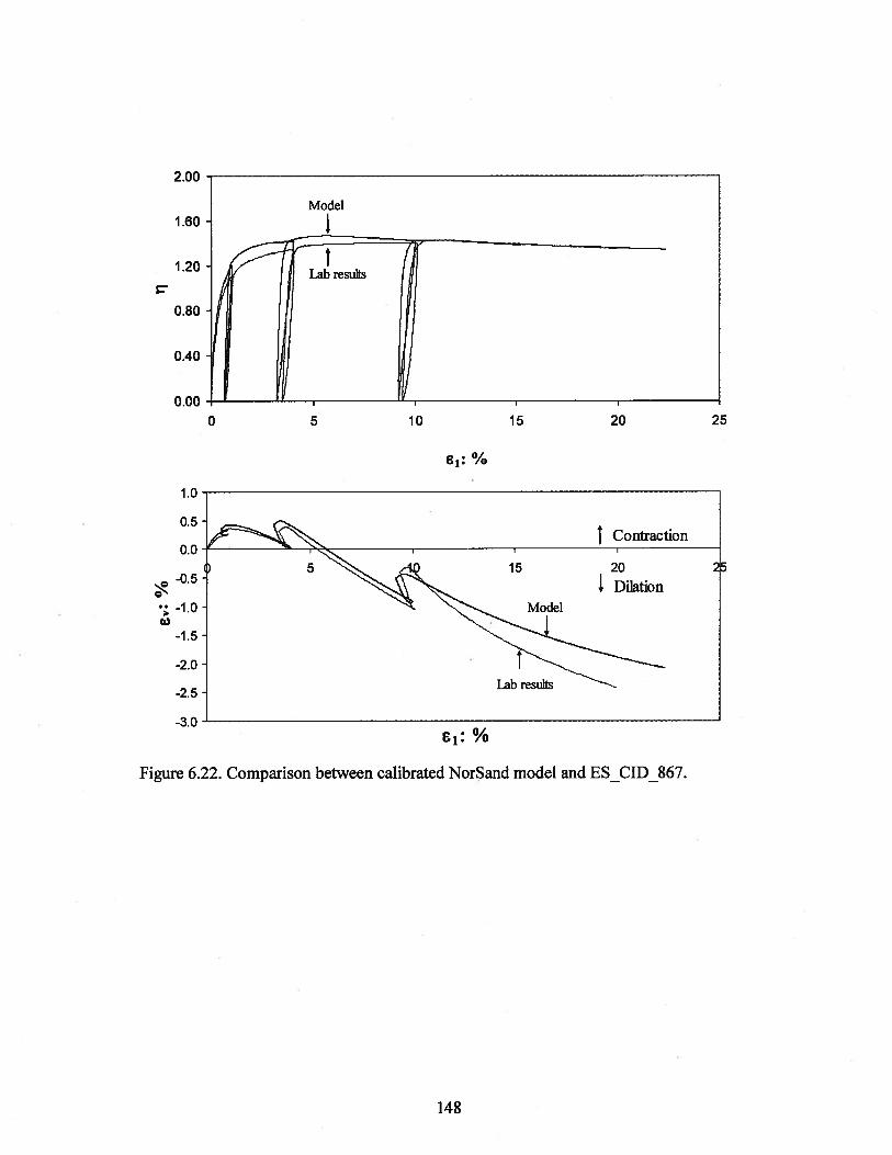
2.00
Model1.60 1
o.ooO1IO2’O 25
61: %
1.0 ——— ——________
0.5Contraction
t
-2.5 Lab results
-3.0s: %
Figure 6.22. Comparison between calibrated NorSand model and ES_CID_867.
148

1.0
w
0.5
0.0
-0.5
Figure 6.23. Zoom on the second ioop of comparison between calibrated NorSand modelwith elasto-plastic unloading and ES_CID_867.
Figure 6.24. Zoom on the second loop of comparison between calibrated NorSand modeland ES_CID_867 with plastic unloading.
8: %
1.0
0.5
0.0
-0.5e1: %
149

0.8
0.6
• 0.40
0.2
0.0
81: %
Figure 6.25. Zoom on the first ioop for ES_CID_867.
6.4. Summary
This chapter presented a triaxial monotonic calibration of the NorSand model to Erksak
sand and Fraser River sand. NorSand requires 8 parameters: 3 critical state parameters, 3
plasticity parameters, and 2 elasticity parameters. The unload-reload model presented in
Chapter 5 requires 3 additional parameters: H, Hr, and %2. An unload-reload calibration
was performed on Erksak sand using cyclic triaxial tests. It was found that Hr and %2 are
related to the monotonic parameters Hand ,j, respectively, such that Hr 4Hand 12 =
1.41i. Hr changes from a value of 4Hto a value ofHonce the yield surface before
unload-reload is exceeded. A constant L[ of 30 fits the unload plots on average.
0 0.5 1 1.5 2 2.5 3
150

7. PREDIcTIoNs OF FRASER RIVER SAND UI4LOAD-RELOAD
BEHAVIOUR
The parameters/relations from the monotonic calibration for Fraser River sand
supplemented by the parameters/relations derived from the unload-reload calibration for
Erksak sand were used to predict the two load-unload-reload triaxial tests on Fraser River
sand using the modified NorSand model developed earlier in Chapter 5. The two triaxial
tests modelled, FR_CID_0l and FR_CID_02 were described in Table 4.4. Test
FR_CID_0l is on a loose sample (pl9OkPa & = 0.012) while test FR CID_02 is on
a dense sample (p’=l98 kPa & yi = -0.156). Both samples were moist tamped.
7.1. Model parameters
As discussed previously in Chapter 6, three additional material parameters are needed
for the proposed unload-reload calibration: “Ha” and ‘H;’, the plastic hardening modulus
in unloading and reloading respectively and X2, the slope of a trend line through the
second peaks of the Dmjn versus yat Dmin data. The same value for H as used for Erksak
sand was assumed (i.e. H = 30). The relation Hr = 4H, derived for the Erksak Sand
calibration, was also used for the reloading portion of the stress path. Hr is used during
loading until the yield surface in existence prior to the current unload-reload is exceeded.
At this point Hr returns to the monotonic loading value of H. The value of X2 for Fraser
River sand was obtained by assuming the same ratio between %i and %2 for Fraser River
sand as obtained from the Erksak calibration. Table 7.1 is a summary of the unload-
reload parameters used for the predictions. The monotonic parameters were presented
previously in Table 6.5.
151

Table 7.1. Parameters used for Fraser River sand unload-reload predictions.
Parameter Erksak sand RemarkH 30 Plastic hardening parameter in
unloadingH,. 4H Plastic hardening parameter in
reloading
Z2 6.12 Slope of the line relating Dmjn toi at Dmjn defined for the secondpeaks
7.2. Model predictions
The updated NorSand model was run using the Fraser River monotonic calibration and
the unload-reload properties/relations derived from the Erksak unload-reload calibration.
No iteration to the input parameters to improve the fits was attempted. The true
measured and NorSand computed stress and strain responses are given in Figure 7.1 and
Figure 7.2 for the loose (FR_CID_01) and dense (FR_CLD_02) tests respectively.
The prediction for FR_CID_0 1 in both q —es and i —j shows slightly lower curves
than laboratory data in the range of 6j values greater than 2% (Figures 7.1 a-b). The
difference between the predictions and the laboratory data starts decreasing at higher
axial strains, i.e.> 15%. Although the predictions and laboratory data for the monotonic
parts of the curves are slightly different, they are very similar in the unload-reload parts.
The slopes of the predicted unload-reload loops are almost identical to those for the
laboratory data. It can be noticed that the area inside the loops is larger at higher axial
strains. The predictions simulate this behaviour.
The model generally predicts more contractive behaviour for FR_CID_01 compared to
laboratory data (Figures 7. ic). Both laboratory data and the predictions are very similar
up to si of around 5%. At higher axial strains, the difference between s from laboratory
152

data and predictions increases with a maximum difference of more than 1% at very high
axial strains.
Similar to FR_CID_01, the monotonic parts of q —8j and —j for the predictions for
FR_CID_02 are slightly lower compared to laboratory data (Figure 7.2a-b). The
difference between the two plots, i.e. laboratory data and predictions, decreases at higher
axial strains close to critical state. The slopes of the unload-reload loops are almost
identical for both the predictions and laboratory data.
The predictions are quite accurate in s, - s for FR CID 02. The maximum difference
between i values for the predictions and laboratory data in-
for FR_CID_02 is
around 0.5% at s = 25% (Figure 7.2c) However, this difference is much smaller at
lower 81 values and the predictions are very accurate. The unload response for the loop
at 8j = 5% is stiffer than the predictions while it is softer for the unload loop at j = 10%.
This is similar to observations for Erksak sand described in Section 6.3.
The area inside the unload-reload loops is larger for FR_CID_02 than that for
FR_CID_0 1. The model captures this behaviour accurately. FR_CID_02 has a higher H
value, and therefore a higher Hr. This yields a stiffer reloading response for FR_CID_02
and the area inside the unload-reload loops is increased.
The predictions for FR_CID_02 in the - plot better match laboratory data than
those for FR_CID_01 (Figures 7.lc & 7.2c). This is because most of the tests used in the
monotonic calibration for Fraser River sand were done on dense samples (see Section
6.2). Therefore, the derived parameters are expected to better fit dense samples. The
predictions are still accurate even for test FR_CIDO1 up to strain levels of around 5%.
In summary, it seems that the unload-reload parameters obtained from the calibration of
Erksak sand provide a reasonably good calibration for Fraser River sand. In q —8j and
17 —8j, the monotonic parts of the plots for the predictions for both tests are slightly lower
than those for laboratory data. However, the slopes of the unload-reload parts are very
153

similar. In a,, — 6j, test FR_CID_02 with the dense sample had better fits than test
FR_CIDO1 with the loose sample. This is expected as the calibration in Chapter 6 was
done using dense samples. Using a constant H value fits the unloading parts on average.
A constant I-Ia results in a simpler calibration although it is evident that unloading is
softer at higher strains.
For future work, other sets of unload-reload tests are needed to better understand the
factors that H depends on. The predictions could be further improved by including more
unload-reload tests on loose samples in the calibration and tests with more unload-reload
loops.
7.3. Discussion of model predictions
To understand the unload-reload behaviour of sands, special laboratory testing
programs that are not commonly performed in industry are required. However,
monotonic laboratory testing is part of the routine in industry. Hence, a model that can
simulate the unload-reload behaviour using unload-reload parameters that can be
correlated to monotonic parameters is of practical significance.
A challenge for any constitutive model is obtaining good quality laboratory information
to calibrate the model. Typically, the simpler the model calibration, the greater the utility
of the model for real engineering problems. This section has investigated whether the
standard monotonic calibration for NorSand, supplemented by relations observed
between the monotonic and three unload-reload parameters for Erksak sand, can be used
to accurately predict the behaviour of a different sand: in this instance Fraser River sand.
Three additional material parameters are needed for the unload-reload calibration: “He”
and H;’, the plastic hardening modulus in unloading and reloading respectively and “X2”,
the slope of a trend line through the second peaks of the Dmjn versus çt’ at Dmin data. From
the unload-reload calibration to Erksak sand presented in Chapter 6, it was shown that Hr
154

and X2 are correlated to the monotonic H and Xi , respectively (Hr 4H & X2 = l.4iXi).
A constant value ofH equal to 30 was shown to fit the unloading curves on average.
The predictions for Fraser River sand presented in this chapter suggest that using
correlations from the Erksak calibration gives quite good fits. The slopes of the predicted
unload-reload loops in q —and i —6j were very similar to those for laboratory data. The
dense sample gave reasonably accurate fits in — 6j plot. The predictions for the dense
sample were better than those for the loose sample. However, the fits for the loose sample
are still quite good up to axial strain of around 5%.
Similar to observation from Erksak data, Fraser River sand simulations show that the
code is not sensitive to changes in H,. because it has a high value of 4H (see Figure 6.19).
As in the Erksak calibration, H of 30 fits the data on average. Changing gives better
predictions. Figure 7.3 shows a model simulation for FR_CID_02 with constant equal
to.
The predictions with changing shown in Figure 7.2b better fit the laboratory data.
It can be seen both simulations (i.e. changing and constant ) are identical up to e of
around 5%. This is because the reloading loops in that range are pre-peak (i.e. start from
pre-peak conditions) and therefore both simulations are based on = 4.34. The later
reloading loops start from post-peak conditions and therefore % changes to 6.12 for the
simulation in Figure 7.2c. It is noteworthy that changing gives identical predictions as
constant,
for FR_CID_0 1 as it is a loose test that never reaches peak.
Overall, the results of the prediction are promising. The current correlation between
monotonic and unload-reload parameters was undertaken based on the triaxial tests for a
single sand, Erksak. It is likely that these correlations will be improved as the database of
triaxial tests with high resolution measurements of the unload reload behaviour expands.
However, where possible it is best to calibrate the unload-reload response directly. A few
triaxial tests with unload-reload loops should be done for more accurate results.
155

7.4. Summary
The standard monotonic calibration for NorSand, supplemented by relations observed
between the monotonic and the three unload-reload parameters for Erksak sand, was
successfully used to predict the cyclic behaviour of another sand: in this instance Fraser
River sand. The main finding of this chapter is that the unload-reload behaviour can be
simulated using unload-reload parameters that can be correlated to monotonic
parameters. It is likely that these correlations will be improved as the database of unload
reload tests expands.
156

(a) 600Test data
_______
500 1400
Predictioi
300
Fraser River sand200e0 =0.89
100 p’l9OkPa
0 I
0 5 10 15 20 25
6j ..%(b)
2.0
Test data1.6
1.2
0.8
0.4
0.0
0 5 10 15 20 25
8j %(c)
4.
Prediction
2
tatafcI
Dilative
0- I I
Figure 7.1. Predictions for Test FR_CID_0 1 (a) q—8j (b) i —si (c) s—8i.
157

(a)1000
_____
Test data800
c 600
400
Fraser River sand
= 0.72200
= 198 kPa0
0 5 10 15 20 2561: %(b)
2.0Test data
1.6
12
0.8
0.4
0.0
0 5 10 15 20 25
61: %(c)
IContractive°
Prediction
-4
-5
-6
Figure 7.2. Predictions for Test FR_CID_02 (a) q—ei (b) i —6j (c)
158

Nabth
E1: %
Figure 7.3. Model simulation for Test FR_CID_02 in 6—6i with constant,‘
of 4.34.
159

8. SUMMARY AND CONCLUSIONS
8.1. Context of Research
The behaviour of sands during loading has been studied in great detail. However, little
work has been devoted to understanding the response of sands in unloading. This is
surprising as the behaviour of sands in unloading is of great practical importance for
earthquake engineering.
An elastic material is expected to expand upon unloading in a conventional triaxial test.
Drained triaxial tests indicate that, contrary to the expected elastic behaviour, sand may
exhibit contractive behaviour when unloaded. Drained cyclic simple shear tests show
similar behaviour in unloading (Sriskandakumar, 2004). Therefore, it is clear that soil
behaviour in unloading is not wholly elastic. The drained behaviour of sands in
unloading was investigated in this work as well as strength and deformation
characteristics in reloading. A practical continuum model that accounts for inelastic
unloading (i.e. yields in unloading) was introduced.
The tendency to contract upon unloading during an earthquake could result in
liquefaction. Undrained cyclic simple shear tests show that the increase in pore water
pressure generated during the unloading cycle often exceeds that generated during
loading. A model that yields in unloading is needed to predict this behaviour.
160

8.2. Research Objectives
The main objectives of this research were:
1. Develop a theoretical understanding of stress-dilatancy in unloading. This
investigation includes the interaction between soil fabric and stress-dilatancy.
2. Utilize the theoretical understanding to guide development of unload-reload
behaviour, including yielding during unloading, into a constitutive model.
8.3. Methodology
The theoretical approach followed is based on Rowe’s stress-dilatancy (Rowe, 1962).
The introduced unload-reload model adopted the NorSand soil model (Jefferies, 1993;
Jefferies and Shuttle, 2005) as its starting point. The flow rule used in the model was
based on observations from a series of triaxial tests with unload-reload loops on Erksak
sand. Calibration of the model for monotonic and unload-reload stress path were
performed for Erksak sand. To determine whether the monotonic to unload-reload
relations observed from the Erksak unload-reload calibrations could be applied generally,
a prediction for unload-reload on Fraser River Sand was undertaken. First a monotonic
calibration of NorSand to Fraser River sand was done. Then the monotonic calibration on
Fraser River sand and the unload-reload parameters for Erksak sand were used to predict
the results of triaxial tests with load-unload-reload cycles on Fraser River sand.
8.4. Conclusions
The theoretical study of deformation characteristic of an assembly of rigid rods shows
that the observed soil contraction in unloading is to be expected. The relation between
stress and dilatancy during unloading depends on particle arrangement. As the
161

arrangement of particles is expected to change with cyclic loading, the stress-dilatancy
relation in reloading differs from that for first loading.
The study of ten drained conventional triaxial tests on Erksak sand, including between
one and three unload-reload loops, indicates that significant amounts of contraction can
occur during unloading. This is contrary to the dilatant elastic unloading response often
assumed in constitutive models of soil. This observed behaviour is consistent with the
results of the theoretical study.
Experimental observations indicate that unloading loops starting from pre-image stress
ratio are dominated by small amounts of dilation, while those starting from post-image
stress ratio are dominated by significant amounts of contraction. The effect of the
unload-reload loops on peak strength is small. This observed contraction in unloading
can be explained based on the saw-tooth model. The sawtooth model suggests that the
more soil dilates in loading, the more potential energy the soil stores. This energy is
available to be released as contraction in subsequent unloading, as observed
experimentally.
The results of the series of tests on Erksak sand show that soil becomes more dilatant in
post-peak reloading phases (i.e. reloading loops occurring post-peak). However, the
stress-dilatancy relation remains as in first loading for pre-peak reloading loops.
The NorSand constitutive model was extended to represent the experimentally observed
yielding during unloading. The introduced model uses non-associated flow in unloading.
Dilatancy in unloading is a function of s1ress ratio, , and the stress ratio (q/p at zero
dilatancy in unloading, M. Soil is assumed to yield in unloading on a vertical cap at
Dmgn. This assumption fits the framework of monotonic NorSand and is consistent with
observations from laboratory data. The cap contracts in unloading dragging the outer
yield surface with it. As a result the outer yield surface softens due to yield in unloading.
162

The resulting model requires the standard 8 NorSand monotonic parameters (T, 2, M,
H, Zic,, N, ‘r,and v). It also requires three additional unload-reload parameters introduced
in this work: “Ha” and “Hr”, the plastic hardening modulus in unloading and reloading
respectively and “X2”, the slope of a trend line through the second peaks (i.e. for post-
peak reloading phases) in Dmjn - çvplot. X2 is used to capture the effect of induced
changes in particles arrangement on stress-dilatancy when stress conditions exceed peak.
The results of the calibration show that the model captures the details of the behaviour
of sand under load-unload-reload cycles. H was significantly smaller than the
monotonic loading hardening, H, and the constant value of 30 provided good fits to the
experimental unload-reload data on average. The code is not sensitive to changes in H,.
because it has a high value of around 4H. %2was always observed to be higher than %
and for Erksak sand%2exceeded Xi by 40%. The calibrated model predicted the results
of triaxial tests with load-unload-reload cycles on Fraser River sand with good precision.
Overall, this thesis introduced stress-dilatancy relations for unloading and reloading
based on experimental observation, supported by the findings of an investigation done at
the micro-mechanical level. An elasto-plastic continuum model that yields in unloading
was proposed. It was shown that the unload-reload behaviour can be simulated using
unload-reload parameters that can be correlated to monotonic parameters.
8.5. Suggestions for Future Work
In summary, this research presents a practical model for load-unload-reload cycles on
sand that incorporate inelastic unloading. It accounts for induced changes in particle
arrangement. The model gives accurate predictions for triaxial Laboratory data. This
research is limited to a triaxial compression framework. For future research, the
proposed model can be implemented in a finite elements code and therefore it needs to be
163

validated for general stress path conditions. An example of this would be a stress path
with decreasing mean effective stress at constant shear stress.
164

REFERENCES
ASTM 2006a, “Standard test methods for maximum index density of soils using a
vibratory table (D4253-00-2006), In 2006 Annual Book of ASTM Standards, sect. 4,
Vol. 4.08, ASTM, Philadelphia.
ASTM 2006b, “Standard test methods for minimum index density of soils and calculation
of relative density (D4254-00-2006), In 2006 Annual Book of ASTM Standards, sect.
4, Vol. 4.08. ASTM, Philadelphia.
Been, K., and Jefferies, M., 1985, “State parameter for sands”, Geotechnique, Vol. 35,
No. 2, pp. 99-112.
Been, K., Jefferies, M., and Hachey, J., 1991, “Critical state of sands”, Geotechnique,
Vol. 41,No. 3,pp. 365-381.
Bishop, A. W., 1971, “Shear strength parameters for undisturbed and remoulded soil
specimens”, Proc. Roscoe Memorial Symp., Cambridge, 3-58.
Bolton, M. D., 1986, “Strength and dilatancy of sands”, Géotechnique, Vol. 36, No. 1,
pp. 65-78.
Byrne, P., Cheung, H., Yan, L., 1987, “Soil parameters for deformation analysis of sand
masses”, Canadian Geotechnical Journal, Vol.24, pp. 366-376.
Casagrande, A., 1936, “Characteristics of cohesionless soils affecting the stability of
earth fill”, Journal of Boston Society of Civil Engineers, Vol. 23, pp. 257-276.
165

Chillarige, AnnajiRao, V., Robertson, P., Morgenstem, N., and Christian, H., 1997,
“Evaluation of the in situ state of Fraser River sand”, Canadian Geotechnical
Journal, Vol. 34, No. 4, pp. 510-519.
Collins, I. F., 2005, “The concept of stored plastic work or frozen elastic energy in soil
mechnics”, Géotechnique, Vol. 55, No. 5, pp. 373-382.
Drucker, D. C., 1951, “A more fundamental approach to stress-strain relations”, Proc.
First US National Congress of Applied Mechanics, ASME, pp. 487-49 1.
Drucker, D. C., and Seereeram, D., 1987, “Remaining at yield during unloading and other
unconventional elasto-plastic response”, Journal of Applied Mechanics, Vol. 54, No.
1, pp. 22-26.
Duncan, J. M., and Chang, C., 1970, “Nonlinear analysis of stress and strain in soils”,
Journal of the Soil Mechanics and Foundations Division, Vol. 96, No. 5, pp. 1629-
1653.
Golder Associates, 1987, “Report on unload testing to assess initial fabric of Erksak
sand”, Golder Associates, Calgary, Alberta
Golder Associates. Erksak 330/0.7 triaxial tests, available at www.golder.com/liq.
Ghafghazi, M., and Shuttle, D., 2006, “Accurate determination of the critical state
friction angle from triaxial tests”, Proc. 59th Canadian Geotechnical Conference,
Vancouver, BC., Canada.
Ishihara, K., Okada, S., 1978, “Yielding of overconsolidated sand and liquefaction model
under cyclic stresses”, Soils and Foundations, Vol. 18, No. 1, pp. 57-72.
Jefferies, M., 1993, ‘NorSand; a simple critical state model for sand” Géotechnique, Vol.
43,No. “pp. 91-103.
166

Jefferies, M., 1997, “Plastic work and isotropic softening in unloading” Geotechnique,
Vol. 47, No. 5, pp. 1037-1042.
Jefferies, M., and Been, K., 2000, “Implications for critical state theory from isotropic
compression of sand” Geotechnique, Vol. 50, No. 4, pp. 419-429.
Jefferies, M., and Been, K., 2006, “Soil liquefaction: A critical state approach”, Taylor &
Francis, London and New York.
Jefferies, M., and Shuttle, D., 2002, “Dilatancy in general Cambridge-type models”
Géotechnique, Vol. 52, No. 9, pp. 625-638.
Jefferies, M., and Shuttle, D., 2005, “NorSand: Features, calibration and use”,
Geotechnical special publication No. 128, American Society of Civil Engineers,
United States, pp. 204-236.
Li, X., and Dafalias, Y., 2000, “Dilatancy for cohesionless soils” Geotechnique, Vol. 50,
No. 4, pp. 449-460.
Mitchell, J., and Soga, K., 2005, “Fundamentals of soil behavior”, 3’ edition, John Wiley
& sons, New Jersey, USA.
Nova, R., 1982, “A constitutive model for soil under monotonic and cyclic loading”, in
Soil Mechanics Transient and Cyclic Loads, Wiley, pp. 343-373.
Oda, M., 1972, “Initial fabrics and their relation to mechanical properties of granular
material”, Soils and Foundations, Vol. 12, No. 1, pp. 17-37.
Palmer, A. C., 1967, “Stress-strain relations for clays: Energy theory”, Géotechnique,
Vol. 17, No. 4, pp. 348-358.
Reynolds, 0., 1885, “On the dilatancy of media composed of rigid particles in contact,
with experimental illustrations”, Philosophical Magazine, Vol. 20, pp. 469-48 1.
167

Roscoe, K., Schofield, A., and Wroth, C., 1958, “On yielding of soils”, Géotechnique,
Vol. 8, No. 1, PP. 22-53.
Roscoe, K., and Burland, J., 1968, “On the generalised stress-strain behaviour of wet
clay”, Engineering Plasticity, Cambridge University Press, Cambridge, pp. 535-609.
Rowe, P. W., 1962, “The stress-dilatancy relation for static equilibrium of an assembly of
particles in contact’, Proc. of the Royal Society, A269, 500-527.
Rowe, P. W., 1969, “The relation between the shear strength of sands in triaxial
compression, plane strain and direct shear”, Géotechnique, Vol. 19, No. 1, pp. 75-86.
Schofield, A. N., and Wroth, C. P., 1968, “Critical state soil mechanics”, McGraw-Hill,
London.
Sasitharan, 5., 1989, “Stress path dependency of dilatancy and stress-strain response of
sand”, M.A.Sc Thesis, University of British Columbia, Vancouver, BC, Canada.
Sriskandakumar, 5., 2004, “Cyclic loading response of Fraser River sand for validation of
numerical models simulating centrifuge tests”, M.A. Sc Thesis, University of British
Columbia, Vancouver, BC, Canada.
Tatsuoka, F., and Ishihara, K., 1974, “Yielding of sand in triaxial compression”, Soils
and Foundations, Vol. 14, pp. 63-76.
Terzaghi, K., Peck, R., and Mesri, G., 1996, “Soil Mechanics in Engineering Practice”,3rd edition, John Wiley & sons, New York, USA.
Vaid, Y. ,and Sasitharan, 5., 1992, “The strength and dilatancy of sand”, Canadian
Geotechnical Journal, Vol. 29, No. 3, pp. 522-526.
Vesic, A. S., and Clough, G., W., 1968, “Behavior of granular materials under high
stresses”, Journal of the Soil Mechanics and Foundations Division, Vol. 94, pp. 661-
688.
168

Wijewickreme, D., Sriskandakumar, S., and Byrne, P., 2005, “Cyclic loading response of
loose air-pluviated Fraser River sand for validation of numerical models simulating
centrifuge tests”, Canadian Geotechnical Journal, Vol. 42, No. 2, pp. 550-561.
Wood, D. M., 1990, “Soil behaviour and critical state soil mechanics”, Cambridge
University Press, Cambridge, UK.
Yasufuku, N., Murata, H., and Hyodo, M., 1991, “Yield characteristics of anisotropically
consolidated sand under low and high stresses”, Soils and Foundations, Vol. 31, No.
1, pp. 95-109.
169

APPENDIX A: PREDICTION OF STRESS DILATANCY IN UNLOADING
It is assumed that stress-dilatancy in unloading can be represented by Equation A. 1.
This appendix presents a quantitative justification using the available data on Erksak sand
(Table 4.2). Figures A.1 to A.1O show a comparison between Equations A.1 to A.3 and
laboratory data.
D°=ii—M (A.l)
Where,
= 2iL —1.5 (A.2)
Where 27L is the last value of stress ratio from the previous loading phase. Plastic
dilatancy in unloading becomes constant at:
D =0.5—Ma (A.3)
Note that the fits for the unload/reload loops at low stress levels are not presented in the
following figures. Those loops are highly influenced by elasticity. Using plastic dilatancy
relation to fit those loops would give inaccurate results. It is assumed that the effect of
elasticity is negligible for the unload/reload loops at higher stress levels.
170

1 4 • Loading I
-s Unloading I
-- •Loading2
U -• •
• : -
- - - -
- :
-
- Model fit to UI
II -- 0.4
0.2
-1.5 -1 -0.5
D
0 0.5
Figure A. 1. Predicted and measured stress-dilatancy for ES_CID_860.
• Loading I1.6
a Unloading 1
Loading 2 -
x Unloading 2 - - )< -
z Loading 3 x - - -- a
U 0.8- -
- Model fit to UI -- - IandU2
• 0.6U
‘a 0.4K.;’ I,
0.2a’_,
-1.5 -I -0.5 0 0.5
D
Figure A.2. Predicted and measured stress-dilatancy for ES_CID_86 1.
171

• Loading 11.6 -
• Unloading 1
•‘z’;’ x Loading 2
• - x Unloading 2• __ ‘—
-- I Loading 3
• -‘- x
: - - - - -
X 0.8 • Unloading 3
- - 0.6 + Loading 4
:- - : x4 - - - Model fit to
t •0.4 • • U2 and U3
-1.5
L0.2 ‘a.
1.5
Figure A.3. Predicted and measured stress-dilatancy for ES_CID_862.
• Loading 1I
a Unloading 1 -
Loading2-
Unloading2 x
Loading 3 x0.8
—— ,.4
- -- ModelfittoUl j 0.6 4.
andU2
C’ E. .
•
-1.5 -1 -0.5 0 0.5 1
D
Figure A.4. Predicted and measured stress-dilatancy for ES_CID_866.
172

4 t?
D
Figure A.5. Predicted and measured stress-dilatancy for ES_CID_867.
D
Figure A.6. Predicted and measured stress-dilatancy for ES_CID_868.
• Loading I
• Unloading 1
Loading 2
x Unloading 2
Loading 3
• Unloading 3
+ Loading 4
-- Model fit for U2 and U3
...‘,•• - -
0.8
0.6•I_ •a : 04’
— —— ..
4;.,•
I -- ••
x
41E •
-2 -1.5 -1 -0.5 0 0.5 1
• Loading 1• Unloading 1e Loading 2x Unloading 2 x
X
x Loading 3 x X
- -- Model fitto UI andU2 X - -
0.6
;‘ 0.4a
0.2
x•
x
c-1.5 -1 -0.5 0 0.5 1
$C A
173

__
-_
_
- - . Loading 1Unloading I
x Unloading 2I - - + Zz Loading 3
xX
+ . Unloading 3
•‘- 0.8 +:,_ + Loading 4
- - X - -- Model fit to U3
- 0.6x> 0.4 -
ci’0.2
-I .- .
-1.5 -1 -0.5 0 0.5
D
Figure A.7. Predicted and measured stress-dilatancy for ES_CID_870.
1.4 - . Loading 1-
. Unloading ILoading 2
•a ‘1 - - - Model fit to Ui
0.6 -
-1.5 -1 -0.5
D
::
Figure A.8. Predicted and measured stress-dilatancy for ES_CID_87 1.
174

D
Figure A.9. Predicted and measured stress-dilatancy for ES_CID_872.
D
A I
1
Figure A. 10. Predicted and measured stress-dilatancy for ES_CID_873.
• Loading 1 4• Unloading I
Loading 2x Unloading 2x Loading3
- - - ModelfittoUlandU2 0.84,, 0.6
0.4
0.2
Es)
-1.5 -1 -0.5 0 0.5 1
• Loading I
• Unloading I
i Loading 2
x Unloading 2
x Loading 3
+ Unloading 3
- Loading 4
- -- Model fit to U2 and U3
c
_+1, xX
:“
)X
•. 0.4
+4*
_ —
I I - I
-2 -1.5 -1 -0.5 0 0.5
175

APPENDIX B: RESULTS OF THE UNLOAD-RELOAD CALIBRATION
FOR ERKSAK SAND
This appendix presents a comparison between the calibrated model results for Erksak
sand as compared to triaxial data. The load-unload-reload calibration used to produce
Figures B.1 to B.7 was introduced in Section 6.1.
2.00
1.60
1.20
0.80
0.40
0.00
-2
: %
Figure B. 1. Load-unload-reload calibration results compared to laboratory data forES_CID_860.
0 5 10 15 20 25
176

2.00 — —_____________________________________________
Model
1.60 1’
1.20 Labres
0.80 ,
LIII
0.40
0.00
0 5 10 15 20 25
Ei: %
1•I Contraction
oModel
—1
-2
-3
-4
-5
Figure B.2. Load-unload-reload calibration results compared to laboratory data forES_CID_86 1.
177

2.00Model
120
1sEfl
0.40
0.00 — I
0 5 10 15 20 25
e1: %
t Contraction
Figure B.3. Load-unload-reload calibration results compared to laboratory data forES_CID_862.
178

2.00
Model1.60
1.20
0.80
0 00
iai,resuits_f - I
0.40
0 5 10 15 20 25
ci: %
t Contraction
Mode.
Co
i1Di1aDilation
—1
Lab results
Figure B.4. Load-unload-reload calibration results compared to laboratory data forES_CID_866.
179

2.00 ——-——— — ——___________________________
Model1.60 1
1.20
10 15 20 25
E: %
1.0
0.5t Contraction
-25Labresults
-3.0ei: %
Figure B .5. Load-unload-reload calibration results, compared to laboratory data forES_CID_867.
180

Model
E1: %
0 5 10
2.00
1.60
1.20
0.80
0.40
0.00
2
I
0
15 20 25
CA)
Figure B.6. Load-unload-reload calibration results compared to laboratory data forES_CID_868.
181

2.00 Model
1.60
1.20
0.80
0.40
0.000 5 10 15 20 25
C1: %
2
t Contraction
0
I lilation-2
03-4
-6
-8
Figure B.7. Load-unload-reload calibration results compared to laboratory data forES_CID_873.
182

APPENDIX C: FRASER RIVER SAND MONOTONIC CALIBRATION
RESULTS
600
500
400
300
200
100
0
A monotonic calibration of NorSand for Fraser River sand was introduced in Section
6.2. The tests used in the calibration are presented in Table 4.5. Figures C. 1 to C.6 show
a comparison between the calibrated model results and laboratory data.
0 5 10 15 20 25
8: %
-2
-6
-8
-10
-12
1.0
0.9
0.8
0.7
0.6100 1000
p’: kPa
Figure C. 1. Monotonic calibration results compared to tests data for FR_CID_03
183

2000
0
Sa
0 5 10 15 20 25
6j. %2
0
-2
-4
-6
-8
-10
1.0
0.9
0.8
0.7
0.6
--
— — — —
100 1000
p’: kPa
Figure C.2. Monotonic calibration results compared to tests data for FR_CID_04.
1600
1200
800
400 FR_CID_04
184

2000
de=O.69
1
0
-1
-2C)
-3
-4
-5
C
C
0 5 10 15 20 25
81: %
1600
1200
800
400— FR_CID_05 p’ = 515 kPa
---- ---_
%%%%
—
— -
0.9
0.8
0.7
0.6100 1000 10000
p’ kPa
Figure C.3. Monotonic calibration results compared to tests data for FR_CID_05.
185

300
200
100
0
2
0
-2
-6
-8
-10
0 5 10 15 20 25
8j. %
.%
%%
SL%%
%%%
—--
100
p’: kPa
NorSandFR_CID_06
e0 = 0.75
p’ 5OkPa
I
1.0
0.9
0.8
0.710 1000
Figure C.4. Monotonic calibration results compared to tests data for FR_CID_06.
186

300
250
200
150NorSand e0 0.91100
_____
p’ 388 kPa50 FR_CU_01
00 5 10 15 20 25 30
81: %
400
rM
200
100.1I0
400
300
0
. 200Cs
100
0 100 200 300 400
p’: kPa
Figure C.5. Monotonic calibration results compared to tests data for FR_CU_0 1.
187

600
500
/orSd 082200
100FR_CU_02 p’ = 196 kPa
00 5 10 15 20 25 30
81. %
160
120
z80
40
-40
400
300
200
100
0 50 100 150 200 250 300 350 400
p’: kPa
Figure C.6. Monotonic calibration results compared to tests data for FR_CU_02
188

APPENDIX D: STEPS TO IMPLEMENT THE LOAD-UNLOAD-
RELOAD MODEL IN A CODE
Figures D.1 to D.3 show the steps that can be followed in coding the load-unload-
reload model.
8L) Addelastic strainsand move to
step 1U
1L)Applyplastic shear
strainincrement
2L) CalculateM and the
current plasticdilation rate
6L) Applyconsistencycondition toget the newstress state
5L) Harden!soften the
yield surface
4L) imposethe limit onthe maximumdilation rate
3L) Recoverplastic
volumetricstrains
Figure D. 1. A diagram illustrating loading in NorSand.
7L) Updatestrains and
state
189

5U) Soften theouter yield surface
6U) Add elasticstrains. Then move
to Step 1R forsubsequentreloading
4U) Recoverplastic volumetricstrain increments
from stressdilatancy and
update strains andstate
1U) Get thecurrent location ofthe internal cap for
the last yieldsurface in
loading/reloading.Ifp Pp’ skip
step 2U.
3U) Apply thehardening rule on
the inner yieldsurface (internalcap) and recover
the new stress state
2U) Recoverelastic strains.Yield surface doesnot change. If pbecomes = Poap goto 3U. Otherwise,go directly to 6U.
Figure D.2. Description of unloading in the model.
190

5R) Go to lUforsubsequentunloading
1R) Apply shearstrain increment
3R) Proceed as inloading starting
from 2L. Use X2 ifpeak is exceeded ina previous loading
2R) Recover elasticstrains until yieldsurface defined in
5U is exceeded
Figure D.3. Description of reloading in the model.
4R) If largest pastyield surface isexceeded use Hinstead of Hr
191

APPENDIX E: TRIAXIAL TESTING PROCEDURE
1. Introduction
This appendix briefly presents the triaxial testing procedure and sample preparation
methods followed to produce the results of the triaxial tests presented in Chapter 4. A
more comprehensive description of the testing procedure can be found in Golder, 1987.
The triaxial apparatus used was described in Section 2.2 (Figure 2.13). All tests
reported in Chapter 4 were displacement controlled. Load was applied by a 19mm
diameter stainless steel piston. The load was measured by a load cell. Cell pressure was
measured using a pressure transducer. Volume change was measured using a cylindrical
piston with a linear displacement transducer that was calibrated to measure volume
change.
2. Sample preparation
• Wet pluviation: A sample of air-dried sand is placed in a long neck flask. The flask
is then filled with de-aired water and placed under vacuum. The membrane mould
is filled with de-aired water and the flask is inverted with its neck 25mm above the
bottom of the mould. Sand then flows out of the flask. The side of the mould is
tapped to reach the desired void ratio.
• Most tamping: The sample is tamped in 6 layers. Distilled water is added to air
dried sand to yield water content of 5-6%. 6 equal weights, prepared to give the
desired void ratio, are tamped inside the mould using a tamper with adjustable
stops.
192

3. Testing procedure
• The lower platen is installed and the membrane (0.3mm thick) is attached using
the 0-rings. The split mould is mounted and vacuum is applied to keep the
membrane stretched.
• The sample is prepared using one of the previously described methods.
• The top platen is placed and the membrane is rolled around the platen and
attached with 0-rings. Vacuum is released and a negative pore pressure of 10-
2OkPa is applied. The mould is then removed.
• The sample diameter is measured at 5 locations and height is determined.
• The cell is filled with water. The loading piston is set in contact with the top
platen and then locked. The LVDT is zeroed.
• A cell pressure of 2OkPa is applied while the negative pore pressure is being
released. The change in volume is recorded.
• For moist tamped samples, carbon dioxide is bubbled through the sample for 3
hours. The sample is then flooded with de-aired water from bottom.
• The cell pressure and back pressure are increased gradually by 100 kPa and the
“B” value is measured. The piston is unlocked and the change in height due to
saturation is recorded. The change in volume is also recorded.
• The sample is consolidated hydrostatically by increasing the cell pressure in
increments. The change in height and volume are recorded.
• All transducers are zeroed and the sample is sheared under either drained or
undrained conditions.
• The drainage line is shut and the sample is frozen. The water content and void
ratio are determined using the frozen sample.
193