antonia kalaitzi measurement-based multipath ... · pdf filemeasurement-based multipath...
TRANSCRIPT
Tampere University of Technology
Department of Communications Engineering
Antonia Kalaitzi
Measurement-Based Multipath Characterization for
Indoor GPS Channels
Master of Science Thesis
Subject approved by the Faculty Council on
14th January, 2009
Examiners: Dr. Docent Elena-Simona Lohan
Professor Markku Renfors

Abstract
Tampere University of Technology
Master’s Degree Program in Radio Frequency ElectronicsDepartment of Communications EngineeringKalaitzi, Antonia: Measurement-Based Multipath Characterization for Indoor GPSChannelsMaster of Science Thesis, 69 pagesMay 2009Examiners: Dr. Docent Elena-Simona Lohan and Professor Markku RenforsKeywords: Global Posistioning System (GPS), Scatterer models, fading, In-phase andQuadrature carrier analysis, Pseudolites (PLs).
Due to the progress of the chip technology and the processing power, the recent GNSSreceivers can provide high positioning accuracy in Line of Sight (LOS) environments.However, in indoor environments (i.e, where LOS is absent) the signal experiences severeattenuation and distortion due to the effect of multipath propagation. In order to be ableto develop better methods to compensate the above mentioned multipath effects, it isimportant to characterize the indoor multipath channel characteristics such as the Timeof Arrival (TOA) distribution, the fading characteristics, the number of clusters and thenumber of paths per cluster. Although one can find several studies in the literature inwhich the TOA behavior is described in wireless indoor environments, no published studyon Pseudolite (PL)-based indoor environment is known, to the best of author’s knowledge.
This thesis makes several contributions, for characteristics both in PL and satellite basedindoor environments. The main contribution of this thesis is the validation of suitableTOA scatterer models to indoor PL-based environments. Secondly, the author suggests acriterion, called Return to low level (RLL), in order to identify the number of clusters andthe number of paths per cluster based on the correlator output of the incoming signal.Thirdly, an attempt is made to set some preliminary thresholds based on the plottedarea of the correlator output, in order to detect the presence of more than one path inpotential multipath scenarios. Finally, the author proposes a unified method for modelingboth small and large scale fading with the use of the Generalized Gamma distribution.
The results of this thesis show that the suggested models can accurately describe thetopology of the scatterers which are used to describe the TOA behavior. Moreover, itwas shown that the proposed RLL criterion can provide good estimates for the number ofclusters and the number of paths per cluster for different indoor environments. Regardingthe multipath identification problem, the results showed that the suggested method wasaccurate even for small Carrier to Noise Ratio (CNR) values. Last but not least, it wasfound that the Generalized Gamma distribution was able to describe the fading amplitudeof the incoming signal both in LOS and non LOS environments.
i

Preface
The present Master of Science Thesis, ”Measurement-Based Multipath Characterizationfor Indoor GPS Channels”, was done in the Department of Communications Engineering,Tampere University of Technology, Finland. This work was carried out in the projectFuture GNSS Applications and Techniques (FUGAT) funded by the Finnish FundingAgency for Technology and Innovation (Tekes), and in the project ”Digital ProcessingAlgorithms for Indoor positioning Systems” (ACAPO) funded by the Academy of Finland.
I would like to express my gratitude to my thesis supervisor Dr. Docent Elena SimonaLohan and Professor Markku Renfors for their valuable guidance, help and support dur-ing the thesis work. I would like also to thank Zahid Bhuiyan for his assistance untilI get familiar with the Latex, Adina Burian, Hu Xuan and Danai Skournetou for theirencouragement during my thesis work.
Finally, I express my gratitude to my family Ioanni, Anastasia, Anna and Georgio for theirhelp and support during my studies abroad.
Tampere, March 27th, 2009
Antonia Kalaitzi
Insinoorinkatu 60 D 31633720 TampereFinlandantonia.kalaitzi(at)tut.fiakalaitz(at)yahoo.grTel. +358 46 892 8335
ii

Contents
Abstract i
Preface ii
Contents iii
List of Abbreviations v
List of Symbols vii
1 Introduction 1
1.1 Short overview of the GNSS system . . . . . . . . . . . . . . . . . . . . . . 1
1.2 Pseudolites . . . . . . . . . . . . . . . . . . . . . . . . . . . . . . . . . . . . 4
1.3 Motivation for the research topic . . . . . . . . . . . . . . . . . . . . . . . . 5
1.4 Related research . . . . . . . . . . . . . . . . . . . . . . . . . . . . . . . . . 6
1.5 Thesis objectives . . . . . . . . . . . . . . . . . . . . . . . . . . . . . . . . . 7
1.6 Thesis contributions . . . . . . . . . . . . . . . . . . . . . . . . . . . . . . . 7
1.7 Thesis outline . . . . . . . . . . . . . . . . . . . . . . . . . . . . . . . . . . . 7
2 Transmission channel model 9
2.1 Propagation mechanisms . . . . . . . . . . . . . . . . . . . . . . . . . . . . . 9
2.1.1 Reflection . . . . . . . . . . . . . . . . . . . . . . . . . . . . . . . . . 9
2.1.2 Diffraction . . . . . . . . . . . . . . . . . . . . . . . . . . . . . . . . 9
2.1.3 Scattering . . . . . . . . . . . . . . . . . . . . . . . . . . . . . . . . . 9
2.1.4 Refraction . . . . . . . . . . . . . . . . . . . . . . . . . . . . . . . . . 10
2.2 Large scale fading . . . . . . . . . . . . . . . . . . . . . . . . . . . . . . . . 10
2.3 Small scale fading . . . . . . . . . . . . . . . . . . . . . . . . . . . . . . . . 11
2.4 Multipath channel parameters . . . . . . . . . . . . . . . . . . . . . . . . . . 11
2.4.1 Mean excess delay . . . . . . . . . . . . . . . . . . . . . . . . . . . . 11
2.4.2 Root mean square delay spread . . . . . . . . . . . . . . . . . . . . . 12
2.4.3 Coherence bandwidth . . . . . . . . . . . . . . . . . . . . . . . . . . 12
2.4.4 Doppler shift . . . . . . . . . . . . . . . . . . . . . . . . . . . . . . . 13
2.4.5 Coherence time . . . . . . . . . . . . . . . . . . . . . . . . . . . . . . 13
2.4.6 Time of arrival (TOA) . . . . . . . . . . . . . . . . . . . . . . . . . . 13
2.4.7 Angle of arrival (AOA) . . . . . . . . . . . . . . . . . . . . . . . . . 14
iii

CONTENTS iv
2.5 Indoor versus outdoor environment . . . . . . . . . . . . . . . . . . . . . . . 14
3 Channel modelling issues 16
3.1 Scatterer models . . . . . . . . . . . . . . . . . . . . . . . . . . . . . . . . . 16
3.1.1 Ring of scatterers (ROS) . . . . . . . . . . . . . . . . . . . . . . . . . 16
3.1.2 Disk of scatterers (DOS) . . . . . . . . . . . . . . . . . . . . . . . . . 17
3.1.3 Elliptical model . . . . . . . . . . . . . . . . . . . . . . . . . . . . . . 19
3.1.4 Circular model . . . . . . . . . . . . . . . . . . . . . . . . . . . . . . 21
3.1.5 Rayleigh model . . . . . . . . . . . . . . . . . . . . . . . . . . . . . . 23
3.1.6 Exponential model . . . . . . . . . . . . . . . . . . . . . . . . . . . . 25
3.1.7 Exponential model of type 2 . . . . . . . . . . . . . . . . . . . . . . 26
3.2 Shadowing/Fading models . . . . . . . . . . . . . . . . . . . . . . . . . . . . 27
3.2.1 Rayleigh distribution . . . . . . . . . . . . . . . . . . . . . . . . . . . 27
3.2.2 Rice distribution . . . . . . . . . . . . . . . . . . . . . . . . . . . . . 28
3.2.3 Weibull distribution . . . . . . . . . . . . . . . . . . . . . . . . . . . 28
3.2.4 Log-normal distribution . . . . . . . . . . . . . . . . . . . . . . . . . 29
3.2.5 Generalized Gamma distribution . . . . . . . . . . . . . . . . . . . . 30
3.2.6 Nakagami distribution . . . . . . . . . . . . . . . . . . . . . . . . . . 30
4 Description of measurement setup 32
4.1 PL-based measurement campaign . . . . . . . . . . . . . . . . . . . . . . . . 32
4.2 Satellite-based measurement campaign . . . . . . . . . . . . . . . . . . . . . 35
5 Selected methodology for indoor channel models 36
5.1 Evaluation of the pdf of TOA from the measurements . . . . . . . . . . . . 36
5.2 Large scale fading information . . . . . . . . . . . . . . . . . . . . . . . . . . 37
5.3 Distribution matching criteria . . . . . . . . . . . . . . . . . . . . . . . . . . 39
5.4 Return to low level (RLL) criterion . . . . . . . . . . . . . . . . . . . . . . . 43
5.5 In-phase and Quadrature carrier phase analysis . . . . . . . . . . . . . . . . 43
6 Results of the measurement data analysis 46
6.1 Measurement-based results about scatterer models . . . . . . . . . . . . . . 46
6.2 RLL-based multipath characterization . . . . . . . . . . . . . . . . . . . . . 49
6.3 Shadowing/Fading models results . . . . . . . . . . . . . . . . . . . . . . . . 49
6.4 I/Q-based multipath detection results . . . . . . . . . . . . . . . . . . . . . 56
7 Conclusions and future work 64
7.1 Conclusions . . . . . . . . . . . . . . . . . . . . . . . . . . . . . . . . . . . . 64
7.2 Future work . . . . . . . . . . . . . . . . . . . . . . . . . . . . . . . . . . . . 65
Bibliography 67

List of Abbreviations
2G Second Generation
3G Third Generation
AOA Angle Of Arrival
AWGN Additive White Gaussian Noise
BPSK Binary Phase Shift Keying
C/A Coarse/Acquisition
CDMA Code Division Multiple Access
cdf Cumulative density function
CNR Carrier to Noise Ratio
CS Commercial Service
DoD Department of Defense
EGNOS European Geostationary Navigation Overlay Service
ESA European Space Agency
EU European Union
FAA Federal Aviation Administration
FCC Federal Communications Commision
FDMA Frequency Division Muliple Access
FUGAT FUture GNSS Applications and Techniques
GEO Geostationary Earth Orbit
GNSS Global Navigation Satellite System
GLONASS GLObal NAvigation Satellite System
GPS Global Positioning Satellite
GSO Geosynchronous Orbit
HP High Precision
IMES Indoor MEssaging System
IRNSS Indian Regional Navigational Satellite System
I/Q In-phase and Quadrature
v

LIST OF ABBREVIATIONS vi
LOS Line Of Sight
MBOC Multiplexed Binary Offset Carrier
MEO Medium Earth Orbit
MSS Mobile Satellite Service
NLOS Non Line Of Sight
OS Open Service
PLs Pseudosatellites
PRN PseudoRandom Noise code
PRS Public Regulated Service
pdf probability density function
RHCP Right Hand Circular Polarization
QZSS Quasi-Zenith Satellite System
SMS Short Message Service
SNR Signal to Noise Ratio
SoL Safety of Life
SP Standard Precision
SSF Space Systems Finland
TOA Time Of Arrival
TUT Tampere University of Technology
WAAS Wide Area Augmentation System

List of Symbols
A Area of scatterer region
α Angle between the major axis of ellipse and the ray from the receiver
αm Semiminor axis of ellipse
Bcoh Coherence bandwidth
bm Semimajor axis of ellipse
β Exponential scatterer model factor
βw Weibull factor
c Speed of light
D Distance between transmitter and receiver
Do Reference distance away from the transmitter
e Generalized Gamma factor
Fs Sampling rate
Fτ (·) Cumulative density function of time of arrival
f Frequency of the electromagnetic wave
fτ (·) Probability density function of time of arrival
fD Doppler shift
fc Carrier frequency
fRayl(·) Rayleigh distribution
fRice(·) Rice distribution
fWeibull(·) Weibull distribution
flogn(·) Log-normal distribution
fGenGamma(·) Generalized Gamma distribution
fNaka(·) Nakagami distribution
g Generalized Gamma factor
γ Pathloss exponent
h Correlator output
I0 Modified 0th order Bessel function
vii

LIST OF SYMBOLS viii
J Correlation envelope
KRice Rician factor
λ Wavelength
µ Mean
m Nakagami factor
Nc Coherent integration length
N Total number of bins
P Mean power level
PT Total power of multipath components
Po Reference mean power level
R Radius of the cell
Rx Receiver
Rr Radius of scatterer model
r Signal level
σ Rayleigh scatterer model factor
σRayl Variance for Rayleigh distribution
σRice Variance for Rice distribution
σLogn Variance for Log-normal distribution
σD Exponential of type 2 model factor
Ts Resolution delay
Tcoh Coherence time
Tx Transmitter
τ Time delay
τm Maximum time delay
τ Mean excess delay
τrms Root mean square delay spread
υs Satellite speed
υr Receiver speed
Wc Cluster width
X Envelope of the incoming fading signal
φ Phase difference between the LOS and the first multipath component

Chapter 1
Introduction
This chapter gives an introduction to the thesis, starting with the Global NavigationSatellite System (GNSS) overview and moving on with the motivation to investigate thecurrent research topic. Finally, the first Chapter ends up by stating the objective, thecontributions and the outline of the thesis.
1.1 Short overview of the GNSS system
The GNSS is an umbrella term for a system of systems including the USA’s Global Po-sitioning System (GPS), the Russia’s GLObal NAvigation Satellite System (GLONASS),the global navigation system built by the European Union (EU) and European SpaceAgency (ESA) GALILEO and the China’s COMPASS [1]. The rest of the existing satel-lite systems are regional and they are used to enhance the performance of the existingGPS, apart from the Indian Regional Navigational Satellite System (IRNSS).
The GPS is a satellite radio navigation system developed by the Department of Defense(DoD) of the USA. The first version of the GPS was called TRANSIT and it consistedof six satellites that could provide worldwide coverage every 90 min and accuracy of 200m. TRANSIT’s technology was strongly related to the Soviet Union’s satellite technologyand it could estimate the position on the ground by measuring the Doppler shift of thesignal. TRANSIT was effective, but it was limited by low accuracy and lack of 24-houravailability [2]. Very soon the DoD decided to develop an improved satellite system andcame up with the GPS which its first operational satellite system was launched in 1978.The GPS now consists of 32 satellites with the 30 operational satellites of the followingtypes [3]: 15 satellites of Block IIA, 12 satellites of Block IIR and 3 satellites of BlockIIR-M. The satellites are distributed in 6 orbital planes with an inclination of 55o relativelyto the equatorial plane, the orbit is nearly circular with a radius equal to 26650 km and aperiod of 12 hours. The satellites on Blocks IIA and IIR send the standard GPS signals,the Coarse/Acquisition (C/A) code on the L1 band with center frequency equal to 1575.42MHz and the P(Y) code for DoD-authorized users only, on the L1 and L2 bands (1227.60MHz). The satellites of Block IIR-M send military signals on L1 and L2 (L1M and L2M)bands and a civil signal on L2 (L2C) band. The GPS is based on Code Division MultipleAccess (CDMA) technique to send different signals on the same radio frequency modulatedby the Binary Shift Phase Keying (BPSK) modulation [4]. The accuracy in civilian GPShas been enhanced from 100 m to 10 m.
1

CHAPTER 1. INTRODUCTION 2
The GLONASS is a radio-based satellite navigation system initially created for militarypurposes. It is the Soviet’s second generation satellite navigation system. The developmentof the GLONASS started in 1976 with a goal of global coverage by the end of 1991. Startingin 1982 and completing the constellation in 1995, the GLONASS felt into decay due to thecollapse of the Russian economy. By 2001 only 8 out of 26 satellites remained in GLONASSorbit. In order to change this situation, Russia decided to restore the systems by 2011 [4].The second updated and current generation of satellites known also as GLONASS-M willbe ready by 2011, the GLONASS-K satellites are the third generation satellites and theGLONASS-KM the fourth generation respectively. By the year 2025 the total number ofsatellites composing the GLONASS constellation will be equal to 24 in total, separated inthree orbital planes with ascending nodes 120o apart and of altitude equal to 19100 km.The orbital period will be 11 hours and 15 min. Each satellite will be able to transmit twotypes of signal: the Standard Precision (SP) signal and the High Precision (HP) signal.The HP signal is mainly used for military purposes. All satellites transmit the sameSP signal, however, each satellite transmits on a different frequency using the FrequencyDivision Multiple Access technique (FDMA). The accuracy of GLONASS navigation basedon the SP signal is 50 to 70 m, while for the HP signal it is 10 m [4].
The European satellite navigation system GALILEO is expected to be fully operationalby the 2013. It will consist of 30 satellites at the altitude of 23222 km, positioned on threecircular Medium Earth Orbit (MEO) planes at a nominal average orbit of 29601.297 km,and at an inclination of the orbital planes of 56o with reference to the equatorial plane. TheEuropean GNSS approach began with the European Geostationary Navigation OverlayService (EGNOS), which provides civil complementary signals to GPS and CLONASSsince the mid-2005 [4]. Once the GALILEO system is completed it will be able to providethe following services:
• The Open Service (OS) will be free for every user. The OS signals will be broadcastin two bands, at 1164 - 1214 MHz (E5 band) and at 1563 - 1591 MHz (E1 band).Receivers will be able to achieve higher accuracy comparable to what the civilianGPS C/A service provides today.
• The Commercial Service (CS) will be available only with a user fee and it providesan accuracy better than 1 m. The CS can also be improved by ground stationsenhancing the accuracy even more to 10 cm.
• The Public Regulated Service (PRS) and Safety of Life service (SoL) will both pro-vide accuracy comparable to the OS. It will be mainly connected with safety-securityapplications.
In 1980 China decided to build an independent satellite system that is expected to befully operational by 2010. China sent three COMPASS navigation test satellites intoorbit between 2000 and 2003. The launch of the two BEIDOU (COMPASS first version)satellites, scheduled in 2007 and covered the whole China and regions around it. The finalconstellation of the GLOBAL satellite system COMPASS will consist of 5 GeostationaryEarth Orbit (GEO) satellites and no more than 30 MEO satellites. By the end of the 2010COMPASS should be able to provide the following services [5], [6]:

CHAPTER 1. INTRODUCTION 3
1. Global Services:
• The OS will be free for every user, providing accuracy equal to 10 m and timingaccuracy within 50 ns.
• The Authorized Service for authorized users ensuring high reliability in com-munications services even in severe conditions, providing timing accuracy of 10ns.
2. Regional Services:
• Wide area differential service, providing accuracy equal to 1 m.
• Short Message Service (SMS) between the COMPASS network and the wireless2G or 3G networks.
Apart from the GNSS there are also other operational satellite systems that do not provideglobal coverage, they are also known as regional satellite systems and they are the followingfour:
1. The Japan’s Quasi-Zenith future Satellite System (QZSS): The QZSS, developedby the Japan aerospace exploration space agency, serves as enhancement of GPSin Japan. The constellation consists of three satellites inclined in elliptical orbitwith different orbital planes. It was designed so as to guarantee that at any timeat least one of the three satellites is close to the zenith over Japan. The QZSSwill make use of the Indoor MEssaging System (IMES) using PseudoRandom Noisecodes (PRN), operated in the GPS L1 center frequency 1575.42 MHz. The IMESwas initially developed to provide indoor positioning accuracy where the GPS or theGNSS signal was not available. An agreement between Japan and USA in Novemberof 2008, ensures that GPS and QZSS will be interoperable and compatible at L1-C/Aand L1C (center frequency 1575.42 MHz), L2C (1227.6 MHz), L5 (1176.45 MHz).The signals of the QZSS will be available in western Pacific Ocean region over Japan.The first satellite out of the three in total satellites will be launched in 2010 [7].
2. The IRNSS: It is expected to be completed by 2012, it is an independent seven-satellite constellation that will be totally constructed and controlled by the Indiangovernment. Three of the satellites in the constellation will be placed in GEO (knownalso as GAGAN) and the remaining four in GeoSynchronous Orbits (GSO) inclinedat 29o to the equatorial plane. IRNSS system provides dual frequency, S and L5band usage with a targeted position accuracy of less than 10 m within India and lessthan 20 m within a region extending approximately 2000 km around it [8].
3. The EGNOS: It is regarded as the first step of Europe’s contribution to the GNSS.It is a satellite-based augmentation system consisting of three GEO satellites and anetwork of ground stations. The EGNOS signal is transmitted by two Inmarsat-3satellites, one over the eastern part of the Atlantic Ocean, the other over the IndianOcean, and the ESA Artemis satellite above Africa. It is able to provide OS for free,for every user promising accuracy of 2 m while it addresses the needs for all modes oftransport including civil aviation, maritime and land users. By 2010 it will be ableto provide SoL applications, while it will be integrated to GALILEO system whenthe later one is ready [9].

CHAPTER 1. INTRODUCTION 4
4. The Wide Area Augmentation System (WAAS): It was created by the Federal Avia-tion Administration (FAA) to augment GPS with additional signals increasing relia-bility, accuracy and availability for the users of USA. It consists of 25 ground stationsand a number of GEO satellites broadcasting signal in GPS band. The WAAS hasmanaged to enhance accuracy from 10 m to 3 m. Each of the 25 ground stationsreceives the signal coming from all the GPS satellites in view. Then the data aresent to the master control from which a satellite message is transmitted to the oneof the GEO satellites. In turn the receiving satellite broadcasts the information toWAAS users [1].
1.2 Pseudolites
Pseudolites, known also as pseudosatellites (PLs), are ground-based GPS transmitters andthey are used when satellite’s signals are not available or when extra ranging signals areneeded. For example regions located in the North Europe with low angle of view to GEOsatellites suffer from reduced GPS coverage. A solution to the above problem can befound with the use of the PLs installed at different elevated locations in either outdoor orindoor environments [10]. The PL idea is older than the GPS system itself. Before thefirst GPS satellites were launched the effectiveness of GPS concept was tested with PLspositioned on high hills in Arizona [11]. Other applications of the PLs apart from theaugmentation of the GPS are the aircraft landing (Horley and Morley, 1997), the Marsexploration (Lemaster and Rock, 1999) and other precision approach applications.
Basically there are two types of PLs, those which are able to receive and transmit rangingsignals in L1/L2 GPS frequencies using either the C/A or the P(Y) code and they areknown as transceivers and those which are not able to generate their own broadcast signalbut they simply act like a mirror and they bounce GPS signals to the receivers, the lasttype of PLs is known as synchrolytes [12]. A problem commonly met in PLs is the so callednear/far problem, that happens when the receiver is either too close to the transmitter orfar away from it. In case the receiver is too close to the PL, the signals coming from otherPLs are blocked, while when the receiver is far away from the PL the transmitted signalcannot be detected. In the present thesis work we did not have to deal with the near/farproblem since only one PL was used in the measurements as it will be discussed later onin the description of measurement setup in Chapter 4. The type of the PL used in all themeasurement scenarios was a transceiver.
Last but not least, PL mutipath has different characteristics compared to the GPS signals.The multipath from PLs is not only a result from reflections taken place on surfaces close tothe transmitter but from the PL itself. For that reason special multipath-limiting antennascan be used to both transmitters and receivers for the elimination of the multipath causedfrom the PL itself. Moreover, in case both the transmitter and receiver are stationarythen multipath effect cannot be mitigated and the noise level of the received signal can beincreased [13]. For all the above reasons special attention is given on multipath effect intelematics applications which include PLs. In the present thesis only the transmitter waskept stationary while the receiver was moving during the measurement’s procedure. ThePLs used in the present thesis work were provided by the Space Systems Finland (SSF).

CHAPTER 1. INTRODUCTION 5
1.3 Motivation for the research topic
In 2003 the Federal Communications Commission (FCC) adopts a stance on Enhanced911 (E-911) requirements for Mobile Satellite Service (MSS) [14]. The requirements setby the FCC, concerning the location information provided with a call made from mobilephones, boosted the interest of the researchers for the development of better wirelesspositioning systems, both cellular and satellite-based. The increased sensitivity of therecent GNSS receivers, based on the progress of chip technology and processing power,has led to high pseudorange accuracy in Line Of Sight (LOS) conditions [15]. On the otherhand, positioning of users located in dense built-up cities and in indoor environments is notso accurate due to the multipath effect which is more severe in such kind of environments,causing the degradation of the positioning services in GNSS applications [16].
In outdoor environments despite the atmospheric effects, there is almost always a directpath between the satellites (at least four satellites are needed for position accuracy) andan outdoor receiver. In indoor environments or in dense and overcrowded towns thisis not the case, while the signal propagates it faces reflections from different scatterersto its way from the transmitting to the receiving antenna. The above procedure is alsoknown as multipath fading phenomenon. Multipath signals are considered undesirable inGNSS technology while they destroy the correlation function shape used for time delayestimation [16]. In addition, multipath propagation causes the fluctuation of the signal’samplitude, phase, angle of arrival (AOA) and time of arrival (TOA) while it travels fromthe transmitter to the receiver. For all the above reasons a characterization of the indoormultipath channel is needed.
Many studies have been carried out in wireless communications and in many differentenvironments in order to estimate the behaviour of TOA of the multipath components.Based on the geometry of the scatterers, in [17] it was proposed an Elliptical and a Circularmodel to describe the topology of the scatterers for indoor and outdoor environments,respectively. In [18] a Rayleigh and an Exponential scatterer model are proposed, inorder to describe the probability density function (pdf) of TOA for both microcellular andmacrocellular environments. In [19] it was proposed the Ring of scatterers and the Diskof scatterers to model the topology of the scatterers around the receiver. All the existingscatterer models have never been applied before this thesis, to the author’s knowledge, onPL-based data.
Furthermore, based on the need for multipath identification in order to describe differentenvironments, the combination of the multipath components grouped in clusters is pro-posed in [20]. Concerning the fluctuation of the envelope of the signal over time, differentstatistical models have been applied for GPS indoor environments. In [21] satellite-basedmeasurements for indoor environment were analyzed, in [22] high bandwidth GPS datawas analyzed in order to characterize fading and multipath characteristics in indoor envi-ronment. The fading behaviour for different indoor environments was investigated in [23]and in [24], based on both PL and satellite measurements. In another important studyin [25] multipath identification was proposed for GPS signals based on the In-phase andQuadrature (I/Q) diagram of the correlator output.

CHAPTER 1. INTRODUCTION 6
1.4 Related research
In [26] a method to extract the large scale fading information from the measurements wasproposed. The basic idea of the method is to average the power of the incoming signalevery 10-80 wavelengths according to the type of the environment. Concerning the L1 bandat the center frequency (1575.14 MHz), 10-80λ corresponds to less than 1 ms, however toour measurements we extended the averaging step up to 100 ms. Until the present thesisthe large scale fading was tested for values 50 ms and 200 ms only [23]. Based on themodified method to evaluate the large scale fading information we managed to encompassboth small and large scale fading in order to apply the Generalized Gamma distribution asit was proposed in [27]. The Generalized Gamma distribution is used to model the fadingeffects. The severity of small and large scale fading can be described from the parametersused in the Generalized Gamma distribution. The results of our measurements in caseof LOS and Non Line Of Sight (NLOS) environments were in accordance with the valuesfound in [28]. In fact, the Generalized Gamma distribution includes also the Rayleigh caseand in case of NLOS scenario, the parameters found for best match with our measurementswere identical to Rayleigh case [28]. Apart from the Generalized Gamma distribution wealso applied the Weibull, the Rice, the Rayleigh and the Nakagami-m distribution in orderto model small scale fading and both small and large scale fading together.
Regarding the scatterer models, the Exponential distribution scatterer model was ableto describe the best the pdf of TOA for indoor PL-based scenarios. The factors thatthe Exponential scatterer model should take into account were: the distance between thetransmitter and the receiver, the radius of the cell and a factor β based on the under-testtype of environment. The model provided in [18] and the assumptions in case of indoorenvironments were proved to be in accordance with our measurement environments as well.A simple Exponential model based only on a factor related to the type of the environmentused, was also tested and performed as well as the Exponential scatterer model, which isin addition of the models reported in [18].
A criterion based on the correlator output of the incoming signal with the local PRN codewas tested to identify the number of clusters and the number of paths per cluster as statedin [20]. The results of our measurements were limited to identify paths of total length lessthan 18.3 m, even though the delay resolution of Ts = 61 ns provided by the samplingrate of Fs = 16.36 MHz used in our measurements was better than those reported in [22].In [22] it was used a delay resolution of approximately 97 ns.
In [22] and [25] it was observed the distortion of the LOS correlation peak due to multipath.In [22] it was proposed a method to reduce the multipath effect. The receiver correlatesthe incoming signal with an internally generated code by using the early and the latecorrelator. The assumed correlator spacing affect the identification of the multipath effectand can be unreliable especially in the presence of noise. On the other hand, in [25] themultipath effect was detected based on the area plotted from the real versus the imaginarycomponent of the correlator output. Based on the same idea we tried to set some thresholdsin order to identify multipath components in case of fading and static channels. Since theidea is new in itself, we could not compare our results with existing results in literature.

CHAPTER 1. INTRODUCTION 7
1.5 Thesis objectives
All the above-mentioned references show that there has been a significant research intereston indoor channel modeling based on GNSS and PL signals, and that there are still severalresearch challenges to be addressed, such as: which are the suitable scatterer models forGNSS/PL signals and which are the statistical characteristics of multipaths (e.g., in termsof fading, multipath delays, etc.).
As a part of the Future GNSS Applications and Techniques (FUGAT) project and ”DigitalProcessing Algorithms for Indoor positioning Systems” (ACAPO) project, the objective ofthis thesis has been to analyze the different measurement data captured from satellites andPLs in various indoor scenarios. The FUGAT and ACAPO projects are research projects,carried out in the Tampere University of Technology (TUT). This thesis covers only asmall part of the research areas of the above projects.
1.6 Thesis contributions
The contributions of the thesis are given below:
• Implementation of existing scatterer models for wireless communications on PL-based measurements.
• Multipath characterization of different indoor environments, identification of numberof clusters and number of multipath components per cluster for PL-based measure-ments.
• Implementation of statistical distributions on PL and satellite-based measurementsin order to evaluate the severity of small and large scale fading.
• An effort to detect the presence of more than one path in the channel, based on theI/Q area of the correlator output.
1.7 Thesis outline
The thesis consists of seven Chapters. The structure of the thesis is given below:
Chapter 1 introduces the motivation of the research topic, related research studies andthe contributions of the present work.
Chapter 2 describes the channel’s characteristics in wireless communications and it givesan overview of signal’s propagation mechanisms and fading.
Chapter 3 presents the scatterer models existing in literature in order to predict the pdfof TOA. Statistical distributions are presented able to describe the behaviour of fading.
Chapter 4 describes the setup of different indoor measurement campaigns based on bothPLs and satellites.
Chapter 5 describes the methodology followed in order to apply the scatterer models andthe statistical distributions. Moreover, it introduces the concepts of the Return to LowLevel criterion and the I/Q area implementation of the correlator output.

CHAPTER 1. INTRODUCTION 8
Chapter 6 presents the results of the thesis. After an overview of the existing scatterermodels and a discussion about their suitability indoors, the Rayleigh and the Exponentialdistribution scatterer models are selected for curve matching. The Exponential distribu-tion scatterer model as well as a simple Exponential model, with parameters set accordingto the environment are proved to be the most suitable for NLOS characterization. Ad-ditionally, fading channel models are applied to describe the behaviour of the small scaleand large scale fading phenomena in both PL and satellite-based measurement scenarios.The parameters of the Generalized Gamma distribution are proved to be a good indicatorof the fading’s severity. Moreover, Rayleigh and Weibull distributions are able to describethe small scale fading. Finally, multipath identification is introduced based on the I/Qdiagram of the correlator output of the received signal with the local PRN code.
Chapter 7 draws the conclusions from this research and makes recommendations forfuture work.

Chapter 2
Transmission channel model
Any wireless system consists of a transmitter, a receiver and a transmission medium.Satellite-based and PL-based navigation systems use air interface as the transmission chan-nel, in which the signal can travel from the transmitter to the receiver over a simple LOSor over multiple reflective paths which is also referred as multipath propagation [29]. Mul-tipath propagation causes fluctuations in the amplitude, the phase, the TOA as well asthe AOA of the received signal. Large scale fading represents the average signal powerattenuation due to motion over large areas. Small scale fading represents the changes inthe amplitude and in the phase of the transmitted signal as a result of small changes inthe spatial separation between the transmitter and the receiver [30]. Basically there arefour types of propagation mechanisms, reflection, diffraction, scattering and refraction.
2.1 Propagation mechanisms
2.1.1 Reflection
Reflection occurs whenever an electromagnetic wave is incident on a smooth surface thenpart of the wave will be reflected. The grazing angle is equal to the reflection angle.When reflection occurs the wave may also be partially refracted, the effect of reflectionand refraction depends on the material’s characteristics, the wave’s polarization, the angleof the incident wave and its frequency [31].
2.1.2 Diffraction
Diffraction occurs when the path of the electromagnetic wave is blocked by an obstaclewith relative sharp edge compared to the wavelength. The diffracted waves are present inthe space and even behind the obstacle. At high frequencies diffraction depends on thegeometry of the object, the amplitude, the phase and the polarization of the incident wave[31]. For the L1 band at center frequency 1575.14 MHz the wavelength is equal to 0.1904m, since λ = c
fwhere c = 3 108 m
sthe speed of light.
2.1.3 Scattering
Scattering occurs when an electromagnetic wave is incident on a rough or irregular surface.The resulting reflections occur in many different directions.
9

CHAPTER 2. TRANSMISSION CHANNEL MODEL 10
2.1.4 Refraction
Refraction occurs whenever an electromagnetic wave is incident on a smooth surface thenpart of the wave will be absorbed by the surface’s material. When refraction occurs thewave may also be partially reflected, the effect of refraction depends on the material’scharacteristics, the wave’s polarization, the incidental wave’s angle and its frequency.
Below in Figure 2.1 are shown the basic propagation mechanisms.
Tx
Scattering
Refraction
Rx
Reflection
Reflection
Diffraction
Figure 2.1: Propagation mechanisms.
2.2 Large scale fading
Large scale fading represents the mean signal power attenuation due to motions over largedistances. This phenomenon is basically affected by obstacles such as hills, forests andbuildings between the transmitter and the receiver. In this case the receiver is beingrepresented as being shadowed by such high obstacles. In overall, the effect of the largescale fading can be expressed through the attenuation of the signal over the distance.Studies are divided into the large scale path loss models and shadow fading models.
In shadow fading models, large scale fading is usually described by Log-normal distribution[29], while the large scale path loss model is given from the Equation below:
10log(Po
P) = 10γlog(
Do
D) (2.1)
where P and Po are the local average power level at distances D and Do respectively, awayfrom the transmitter. The parameter γ used in the formula is called pathloss exponent

CHAPTER 2. TRANSMISSION CHANNEL MODEL 11
and its value is different for different environments. In free space the pathloss exponent isequal to 2 while for denser environments it gets values higher than 2.
2.3 Small scale fading
Due to the multipath effect as the receiver moves over short distances the signal strengthvaries rapidly [32]. This feature is called small scale fading or multipath fading and it canbe explained as following: the instantaneous received signal strength is the sum of thesignals which are reaching the receiver from different directions and with different phasesdue to multipath propagation. Rayleigh and Rician distribution are the most commonlyused small scale distributions in NLOS and LOS scenarios respectively.
The factors which affect the small scale fading are the following [30]:
1. Multipath propagation: It causes different replicas of the transmitted signal toreach the receiver with different amplitude, different phase and different TOA. Therandom phases and amplitudes of the arriving multipath components cause rapidfluctuations to the signal’s strength over time.
2. Receiver’s speed: The motion of the receiver about the transmitter causes randomfrequency modulation to the arriving multipath components.
3. Surrounding objects’ speed: The effect of the speed of the surrounding objectsis the same as in case of the receiver’s speed.
4. Bandwidth of the transmitted signal: The bandwidth of the signal can makethe severity of distortion, which the signal will experience when it passes throughthe multipath channel, to vary.
In order to understand better the effect of the above factors on the small scale fading wehave first to introduce some basic parameters in order to describe and compare differentmultipath channels.
2.4 Multipath channel parameters
2.4.1 Mean excess delay
Assuming the multipath channel has the multipath delay profile as the one shown in theFigure 2.2:
We define as mean excess delay τ :
τ =
K∑
i=1
P (τi)τi
PT
(2.2)
where P (τi) is the relative power of the multipath component at ith delay τi and PT is
the total power of all taps K in total (PT =K
∑
i=1
P (τi)).

CHAPTER 2. TRANSMISSION CHANNEL MODEL 12
Figure 2.2: Delay profile.
2.4.2 Root mean square delay spread
The Root Mean Square (RMS) delay spread is the square root of the second central momentof the power delay profile and it is given from the Equation below:
τrms =
√
√
√
√
1
PT
K∑
i=1
P (τi)τ2i − τ2 (2.3)
where τ is the mean excess delay coming from Equation 2.2. The RMS delay spread takesinto account the mean power level as well as the mean delay of the multipath components.Based on the RMS delay spread a channel is being characterized as narrowband when theRMS delay spread is shorter than the symbol duration. While on the other hand a channelis being characterized as wideband when the RMS delay spread is much larger than thesymbol duration [30].
2.4.3 Coherence bandwidth
The RMS delay spread can be used to define the coherence bandwidth of the channel. Weregard as coherence bandwidth Bcoh, the maximum transmission bandwidth over which thechannel can be assumed to be approximately constant in frequency. The relation betweenthe Bcoh and the RMS delay spread is given below:
Bcoh ∼ 1
τrms(2.4)
If the bandwidth of the signal is smaller than the coherence bandwidth of the channelthen the channel is being characterized as flat fading, in that case all the frequencies ofthe signal experience the same fading. On the other hand, in case the bandwidth of thesignal is larger than the coherence bandwidth of the channel then the channel is beingcharacterized as frequency selective and different frequencies of the transmitted signalexperience different fading.

CHAPTER 2. TRANSMISSION CHANNEL MODEL 13
2.4.4 Doppler shift
The motion of the satellites introduces frequency modulation on the carrier and the codeof the received signal. The frequency modulation due to Doppler shift is expressed fromthe following formula:
fD = fcυs
c(2.5)
where fD is the Doppler shift, fc is the carrier frequency of the transmitted signal, υs isthe speed of the satellite and c is the speed of light. Thus, for a satellite speed equal to3900 m
sat the center frequency of L1 band, the Doppler shift is equal to 20.48 kHz.
This phenomenon results in the Doppler spectrum where the exact shape of the spectrumdepends on the relative amplitudes and on the arriving angles of the incoming multipathcomponents.
Even in case where PLs are used instead of the satellites then Doppler shift remains dueto the motion of the receiver and the Equation 2.5 is transformed to:
fD = fcυr
ccos(ψ) (2.6)
where ψ is the angle between the direction where the motion takes place and the directionof the arrival multipath components in a horizontal plane. The Doppler shift can be eitherpositive or negative depending whether the receiver is moving towards or away from thetransmitting antenna [30]. In case of a pedestrian user with speed equal to 1 m
sand ψ = 0
at L1 center frequency, the Doppler shift is equal to 5.25 Hz.
2.4.5 Coherence time
We regard as coherence time Tcoh, the time duration over which the channel impulseresponse is time invariant. The Doppler shift and coherence time are inversely proportionalto each other.
Tcoh ∼ 1
fD(2.7)
If the coherence time of the channel is less compared to the transmitted symbol durationthen the fading is being described as fast fading, on the other hand when the coherencetime of the channel is bigger compared to the transmitted symbol duration then the fadingis being described as slow fading.
2.4.6 Time of arrival (TOA)
Due to the NLOS error accurate location positioning is still an issue [19]. In most envi-ronments both indoor and outdoor due to the lack of LOS path between the receiver andthe transmitter the measured signal path is always larger that the true LOS path, thatis because of the propagation mechanisms that take place on the signal’s way before itreaches the receiver. For that reason the knowledge of the TOA in accurate positioningsystems is of great importance. Several different scatterer models have been developed inorder to provide the pdf of the TOA [17], [18], [19]. The geometry of the models will bepresented in Chapter 3.

CHAPTER 2. TRANSMISSION CHANNEL MODEL 14
2.4.7 Angle of arrival (AOA)
Another important issue especially in beamforming localization applications is the knowl-edge of the AOA of the multipath components. Below it is shown an example of jointpdf of the TOA and AOA for a typical outdoor environment where the radius of the cellis assumed to be 1000 m and the distance between the receiver and the transmitter isassumed to be 500 m [17].
24
68
x 10−6
−200
−100
0
100
2002.5
3
3.5
4
4.5
5
5.5
Time of Arrival [s] Angle of Arrival [deg]
pd
f (T
OA
/AO
A)
Figure 2.3: Joint TOA/AOA pdf for outdoor environment.
2.5 Indoor versus outdoor environment
In outdoor environment, despite the atmospheric effects and the attenuation they cause,the direct path LOS between the receiver and the satellite is most of the times strongerin amplitude than the NLOS path. The outdoor NLOS signal is delayed compared to theoutdoor LOS and the maximum excess delay can be valued up to 100 µs (or 102.3 chipsdelay) [15]. On the other hand, in indoor environment the LOS can be absent, in additionto that there have been detected cases where the NLOS signal has stronger amplitudethan the LOS. The excess delay in indoor environments is typically less than 1 µs (or1.023 chips delay) [15].
Moreover, the Doppler shift caused by the motion of the receiver in outdoor environmentscan be detected while in indoor environments due to the small accelerations in user’s mo-tions the Doppler shift cannot be easily detected. The result of the above privilege inoutdoor environments is the implementation of more accurate positioning systems com-pared to indoors.
According to [20] the multipath rays arrive at the receiver grouped in clusters. The numberof the multipath components as well as the total amount of clusters differ from outdoorto indoor environment.

CHAPTER 2. TRANSMISSION CHANNEL MODEL 15
In the present thesis the computation of the total amount of clusters as well as the totalamount of multipaths per cluster was done for indoor PL-based environments only, thereason for excluding the satellite-based measurements will be explained in Chapter 5.

Chapter 3
Channel modelling issues
The present Chapter presents the geometry of the scatterer models found in the literature,able to describe the pdf of TOA. Since each model is based on different geometry ofscatterers all the required information is given concerning the type of the environment thatthe model can be applied. Apart from the scatterer models the present Chapter describesthe main statistical distributions able to describe the large and small scale fading. Thepdf and the parameters used for each distribution are discussed and shown in details.
3.1 Scatterer models
3.1.1 Ring of scatterers (ROS)
The ROS model assumes a distribution of scatterers around a ring whose center is thereceiver (denoted as Rx in the following figures). More precisely, the present model assumesa uniform distribution of scatterers within the range [0,2π] around the receiver. The ROSmodel assumes that the scatterers are located on a ring centered about the Rx with aradius equal to Rr. It is mainly a sparse distribution of scatterers around the Rx. TheROS model is applicable in cases where the transmitter (denoted as Tx in the followingfigures) is placed higher than the Rx which is near the ground and surrounded by the localscatterers [33]. The geometry of the ROS model it is shown in the Figure 3.1 and it canbe basically applied to macrocellular environments.
The pdf of TOA of an arriving multipath signal component from a single reflection is givenby the Equation 3.1:
fτ (τ) =τc−Rr
cRrDΩτ
D
c≤ τ ≤ D + 2Rr
c(3.1)
where Rr is the radius of the scatterers around the Rx and c the speed of light. Thereal distance between the Tx and the Rx is denoted as D, but the measured propagationdistance is always larger than the D due to multipath, where D is equal to:
D =
√
((xRx − xTx)2 + (yRx − yTx)2) (3.2)
The value for the variable Ωτ in Equation 3.1 is coming from below:
16

CHAPTER 3. CHANNEL MODELLING ISSUES 17
Figure 3.1: Geometry of the ROS model.
Ωτ =
√
1 − [(D − τc)(D + τc− 2Rr)
2DRr+ 1]2 (3.3)
3.1.2 Disk of scatterers (DOS)
The DOS model is mainly applicable for macrocellural environments. Since the scatteringeffects cannot be described in details they can be modeled on average and this is thepurpose of this model. In this model it is assumed that the scatterers are located ona solid circular disk around the Rx of radius Rr. The assumption for the density ofscatterers may differ from environment to environment, from macrocell to picocell, fromsparse environment to dense environment. The most common approaches concerning thedensity of the scatterers are given in [34], [35] and [36]. Despite the different density models,the Gaussian [36] and the uniform distribution [34] do not provide different results [36].The present DOS model assumes a dense uniform distribution of scatterers around theRx. In Figure 3.2 we can see the geometry of the model.
The pdf of TOA of an arriving multipath component from the Tx to the Rx according to[19] is equal to:
fτ (τ) =Nτ (τ)
cLτ (τ)(3.4)
The parameters Nτ and Lτ are coming from the Equations 3.5 and 3.7,
Nτ (τ) = (−τc2 +D2)(τc− 2Rr) (3.5)
.√
(D + 2Rr − τc)(D − 2Rr + τc)
−2(2τc4 − 3τc2D2 +D4)arctan(Qτ )
Qτ =(τc+D)tan(1
2arccos(τc2+D2−2τcRr
2D(τc−Rr) ))√τc2 −D2
(3.6)

CHAPTER 3. CHANNEL MODELLING ISSUES 18
Figure 3.2: Geometry of the DOS model.
The measured distance in the DOS model is equal to:
Lτ (τ) = 4πR2r(τc−D)
32 (τc+D)
32 (3.7)
In overall, the Figure 3.3 shows the pdf of TOA for different radius for both ROS andDOS models. As we can see for the ROS model the peaks of the pdf of TOA are near thecorresponding LOS distance (D) and the NLOS distance (D + 2Rr, as it was assumed).On the other hand, for the DOS model the multipath pdf of TOA gets high values nearthe LOS distance (D) only.
2 2.5 3 3.5 4 4.5 5 5.5 6 6.5 70
0.005
0.01
0.015
0.02
0.025
0.03
0.035
0.04
Delay [microseconds]
pd
f o
f T
OA
ROS model D=1000m Rr=300mDOS model D=1500m Rr=300mROS model D=800m Rr=200mDOS model D=1300m Rr=300m
Figure 3.3: The pdf of TOA for both ROS and DOS models for different parameters.
There are also other types of scattering models applicable in macrocellural environmentssuch as the Gausssian scattering model which takes into account the variance and themean value of TOA [19]. The formulas used to extract the pdf of TOA for the Gausssianscatterer model are not presented here since they are used in algorithms applicable forNLOS mitigation [19].

CHAPTER 3. CHANNEL MODELLING ISSUES 19
3.1.3 Elliptical model
The Elliptical scattering model assumes an ellipse for the position of the scatterers inwhich the transmitter and the receiver are located at its both foci [37]. This scatteringmodel was proposed for microcellular environments where the antenna height is low andmultipath components are likely to come from points very close to the Rx and the Tx. Theassumed geometry of the Elliptical scattering model is the one shown in the Figure 3.4.The major axis of the ellipse is given from the equation cτm where τm is the maximumdelay associated with the scatterers within the ellipse and c is the speed of light. TheElliptical model considers only those multipath components that arrive at the receiverwith maximum delay of τm, neglecting paths with greater path delays than that. Theprevious assumption can be valid since multipath components that arrive with multipathdelays larger than τm, have less power from those which arrive with path delays smallerthan τm. The attenuation on the power of the multipath components with large pathdelays is due to the greater path loss they experience. Thus, a large value for τm can makethe model perform very well.
The assumptions valid for this model are the following [17]:
• The signals are propagating in the horizontal plane.
• The scatterers are considered as omnidirectional reradiating elements.
• The signals arriving in the transmitter have interacted with only one scatterer.
Figure 3.4: Geometry for the Elliptical model.
Here, the semiminor and semimajor axes of the ellipse are defined as follows:
am =cτm2
(3.8)
bm =1
2
√
c2τ2m −D2 (3.9)

CHAPTER 3. CHANNEL MODELLING ISSUES 20
where D is the distance between the Rx and the Tx. The pdf of TOA even for a simplecase of uniform scatterer density is very difficult to evaluate, for that reason we are goingto derive the pdf throught the cumulative density function (cdf) of TOA. Thus, workingon the area shown in the Figure 3.5 the cdf is given as follows:
Figure 3.5: Region of scatterers needed for the cdf calculation of TOA.
Fτ (τ) =Aτ (τ)
A(3.10)
where A is the area of the scatterer region and Aτ the intersection area as a function ofthe delay τ . Taking the derivative of the above equation with respect to τ we come upwith:
d
dτFτ (τ) =
1
A
d(Aτ (τ))
dτ(3.11)
HereAτ is the scatterer region for a certain delay τ . The intersection area can be consideredin case of the Elliptical model as a small ellipse whose area is given from the Equation3.12.
Aτ (τ) = πaτ bτ =πτc
4
√
(τ2c2 −D2) (3.12)
The parameters aτ and bτ correspond to the semiminor and semimajor axis of the ellipsefor time delay equal to τ . As we said before for the pdf of TOA we need to extract thederivative of cdf, so the derivative of the intersection region with respect to the τ is shownbelow:
d
dτ(Aτ (τ)) =
πc(2τ2c2 −D2)
4√
(τ2c2 −D2)(3.13)
Finally, after some calculations that are explained analytically in [17], the pdf of TOA iscoming from Equation 3.14:

CHAPTER 3. CHANNEL MODELLING ISSUES 21
fτ (τ) =
c(2τ2c2−D2)
4αmbm
√τ2c2−D2
Dc≤ τ ≤ τm
0 else(3.14)
The Figure 3.7 shows typical examples of pdf of the TOA for the Elliptical model.
3.1.4 Circular model
The Circular scattering model is applicable to macrocellural environments where the heightof the antennas is high enough and takes into account a uniform pdf of scatterers lyingaround the receiver [17]. Since the antenna heights are high enough the present modelassumes no signal scattering source from locations next to the Tx. Only one case is beingexamined here, the case where the distance between the transmitter and the receiver ismuch bigger from the radius of the scatterers. The extraction of the pdf of TOA is morecomplex than it was in the Elliptical scatterer model, but we should first represent thegeometry of the model in Figure 3.6. The same assumptions as those used for the Ellipticalmodel are also valid here.
Figure 3.6: Geometry of Circular model.
In order to provide the pdf of TOA we must first calculate the intersection area of theellipse and the circular scatterer region, where the major axis of the ellipse is equal to cτ[17]. The derivative of the uniform scatterer density function with respect to τ will givethe necessary pdf, Equation 3.15.
fτ (τ) =1
A
d(Aτ (τ))
dτ(3.15)
As we can see from the Figure 3.6 the common area of the ellipse and the circular scattererregion is divided into two subareas A1 and A2. The angle between the major axis of theellipse and the ray from the receiver is denoted as α and it is given in the Equation 3.16.
α = arccos(D2 + 2Rrτc− τ2c2
2RrD) (3.16)

CHAPTER 3. CHANNEL MODELLING ISSUES 22
where D is the distance between the transmitter and the receiver and Rr is the radius ofthe circular scatterer region. Now since we know α we can define the whole intersectionarea as a function of τ coming up to Equation 3.17:
Aτ (τ) = R2rα+
D2 − τ2c2
4(3.17)
.[−πτc√τ2c2 −D2
+Dsin(α)
τc−Dcos(a)+
2τc√τ2c2 −D2
.atan(
√τ2c2 −D2tan(α
2 )
τc−D)]
Finally, the pdf of TOA for the circular scatterer model is shown in the Equation 3.18:
fτ (τ) =c
πR2r
(3.18)
.πτ2c2k2 − τck2
2 + πk2k21 + τck2
1 + τck21 − 2Rrk
21
4k1k2
+τ2c2k0k4 + τck0k
21
2k24 + 2k2
0k21
+τ2c2 + k2
1
2k1
.atan(k0k1
k4) − Rr − τc
(4R2rD
2 − k23)
(1/2)
.(2R2r +
τck21k4(1 + k2
0)
2k24 + 2k2
0k21
)
where the k’s values are coming from following Equations:
k0 = tan(1
2acos(
−τ2c2 +D2 + 2Rrcτ
2RrD)) (3.19)
k1 =√
τ2c2 −D2 (3.20)
k2 =√
D2 − 4R2r − τ2c2 + 4Rrτc (3.21)
k3 = −τ2c2 +D2 + 2Rrτc (3.22)
k4 = D − τc (3.23)
The Equation 3.18 for the pdf of TOA is valid when the following condition is beingsatisfied,
D
c≤ τ ≤ D + 2Rr
c(3.24)
In total, the pdf of TOA for both the Elliptical and the Circular models is presented inthe Figure 3.7.

CHAPTER 3. CHANNEL MODELLING ISSUES 23
As we can see in the Figure 3.7, for the Elliptical model the pdf is high enough for smallvalues of the assumed time delay. Increasing the distance between the receiver and thetransmitter the delay increases as well. The upper limit for the representation of pdf asa function of the time delay is given from the factor τm (denoted as taum in the Figure3.7). On the other hand, the Circular model depends on the distance and the radius ofthe scatterer region. The radius of the region affects the maximum value for the delay ofTOA, more precisely the larger the radius the higher the delay.
3 3.5 4 4.5 5 5.5 6 6.5 70
0.1
0.2
0.3
0.4
0.5
0.6
0.7
0.8
0.9
1
Delay [microseconds]
pdf o
f TO
A
Elliptical D=1000m tau
m=6microsec
Elliptical D=1150m taum
=7microsec
Circular D=900m Rr=200mCircular D=990m Rr=300m
Figure 3.7: The pdf of TOA for both Elliptical and Circular scatterer models for differentparameters.
3.1.5 Rayleigh model
It is a geometrically based statistical model that assumes the scatterers are randomlyand non uniformly distributed around the transmitter and within a circle that its areais determined by the antenna’s radiation pattern. It is suitable for outdoor microcellularpropagation environments according to [18]. In this model the transmitter is assumed tobe located in the center of a circular area with the mobile receiver in it as well. ApplyingRayleigh distribution for the scatterers we get the pdf of TOA for the present model. Theassumption that both the transmitter and the mobile receiver are located inside a circle,is valid since multipath components originate from both of them in case of microcellularenvironments. Before going on to the geometry of the model and the derivation of thepdf of TOA, there are some further assumptions for this model that we have to take intoaccount [18]. The first assumption is the fact that we regard every scatterer as an omni-directional reradiating element. Another assumption is that during the propagation pathof a multipath component only one bounce it is assumed. Last but not least, interferencecaused from neighbour cells is neglected. The geometry of the model is shown in theFigure 3.8.
As we can see from the Figure 3.8 the density of the scatterers decreases away from thetransmitter. This assumption is valid in small towns where the density of the buildingsand the scatterers reduces while we are moving away from the center of the town [18].The scatterers that contribute to the same time delay are within an ellipse. The ellipse isexpressed in polar coordinates from the Equation 3.25. The transmitter and the mobilereceiver are both located at the foci of an ellipse inside a cell of radius R. The term cτ

CHAPTER 3. CHANNEL MODELLING ISSUES 24
Figure 3.8: Geometry of Rayleigh and Exponential scatterer model.
expresses the major axis of the ellipse. Inside the circle the ellipse remains for maximumtime equal to 2R−D
c, when that time exceeds the intersection area becomes part of the
ellipse. This model can be applied in cases where either Rayleigh or Exponential distri-bution of scatterers has been assumed [18]. The joint pdf of fpϕ(p, ϕ) expressed in polar
coordinates is given from the equation 3.26, where NR = 1− e−R2
2σ2 . Finally, the cdf of theellipse is coming from the Equation 3.27.
p =c2τ2 −D2 − 2
2cτ + 2RDcosϕ(3.25)
fpϕ(p, ϕ) =p
2πNRσ2e
−p2
2σ2 (3.26)
Fτ (τ) =
2∫ π
0
∫ R
0c2τ2
−D2
2cτ+2Dcos(ϕ)fpϕ(p,ϕ) dpdϕ
∫ 2π
0
∫ R
0 fpϕ(p,ϕ) dpdϕτ ≤ 2R−D
c
2∫ π
a
∫ R
0 fpϕ(p,ϕ) dpdϕ+2∫ α
0
∫ R
0c2τ2
−D2
2cτ+2Dcos(ϕ)fp,ϕ dpdϕ
∫ 2π
0
∫ R
0 fpϕ(p,ϕ) dpdϕτ > 2R−D
c
(3.27)
where a in the Figure 3.8 is equal to:
a = arccos(c2τ2 −D2 − 2Rcτ
2RD) (3.28)
Replacing Equation 3.26 into Equation 3.27 and taking the derivative with respect to τwill give the following pdf of TOA for the Rayleigh model:
fτ (τ) =
∫ π
0 e
C1(cτ+Dcosϕ)2 (
C′
1(cτ+Dcosϕ)2
− 2cC1(cτ+Dcosϕ)3
) dϕ
π(e−R2
2σ2 −1)
τ ≤ 2R−Dc
∫ α
0 e
C1(cτ+Dcosϕ)2 (
C′
1(cτ+Dcosϕ)2
− 2cC1(cτ+Dcosϕ)3
) dϕ
π(e−R2
2σ2 −1)
τ > 2R−Dc
(3.29)

CHAPTER 3. CHANNEL MODELLING ISSUES 25
where C1 is coming from Equation 3.30 and C ′1 is coming from Equation 3.31. The factor
σ depends on the type of the environment we test and it can take any value, in specialcase where the R ≤ σ the pdf of TOA remains the same [18].
C1 =−(c2τ2 −D2)2
8σ2(3.30)
C ′1 =
−(c2τ2 −D2)c2τ
2σ2(3.31)
3.1.6 Exponential model
This model assumes an Exponential distribution of scatterers around the transmitter andit is applicable to indoor environments. The pdf of TOA is derived assuming in polarcoordinate system a distribution of the form, see Equation 3.32.
fp(p) =β
NEe−βρ (3.32)
where NE = 1−e−βR is the normalization constant, ρ belongs to [0, R] and β is a constant.The resulting pdf of TOA for the Exponential scatterer model is given below:
fτ (τ) =
∫ π
0 eC2
cτ+Dcosϕ (C′
2cτ+Dcosϕ
− cC2(cτ+Dcosϕ)2
) dϕ
π(e−Rβ−1)τ ≤ 2R−D
c∫ β
0 eC2
cτ+Dcosϕ (C′
2cτ+Dcosϕ
− cC2(cτ+Dcosϕ)2
) dϕ
π(e−Rβ−1)τ > 2R−D
c
(3.33)
where the values for the parameters C2 and C ′2 are coming from the Equations 3.34, 3.35.
C2 = −β (c2τ2 −D2)
2(3.34)
C ′2 = −βc2τ (3.35)
1 1.5 2 2.5 3 3.5 4 4.5 5 5.5 60
0.01
0.02
0.03
0.04
0.05
0.06
0.07
0.08
0.09
Delay [microseconds]
pdf o
f TO
A
Rayleigh R=1000m D=200m sigma=0.2/RRayleigh R=900m D=180m sigma=0.3/RExponential R=80m D=16m beta=0.8/RExponential R=80m D=16m beta=0.5/R
Figure 3.9: The pdf of TOA for both Rayleigh and Exponential scatterer models fordifferent parameters.

CHAPTER 3. CHANNEL MODELLING ISSUES 26
The pdf of TOA for both models is shown in the Figure 3.9, where the parameter σ ofthe Rayleigh model is denoted as sigma, and the parameter β of the Exponential modelis denoted as beta. In both scatterer models the pdf of TOA at the receiver decreases asthe time increases from the minimum to maximum path delay.
3.1.7 Exponential model of type 2
Among the scatterer models we found in the literature we also tested the suitability ofa simple exponential form as shown in the Equation 3.36, where τ is the time delay inchips (1 chip is equal to 1
1.023∗106 s) and σD is a parameter that is defined according to themeasurement’s environment.
fτ (τ) = e− τ
σD (3.36)
In overall, the characteristics of the scatterer models found in the literature are presentedin the Tables 3.1 and 3.2,
Table 3.1: Scatterer models and their attributes (1)
Scatterer model Main parameters Antenna heights
ROS D, Rr Tx higher than RxDOS D, Rr Tx same as Rx
Elliptical D, τm Tx same as RxCircular D, Rr Tx same as RxRayleigh D, R, σ Tx same as Rx
Exponential D, R, β Tx same as Rx
Table 3.2: Scatterer models and their attributes (2)
Scatterer model Scatterer Type of Omnidirectionaldistribution environment scatterers
ROS Uniform Macrocellular -DOS Uniform Macrocellular -
Elliptical Uniform Microcellular YesCircular Unifrom Macrocellular YesRayleigh Rayleigh Macrocellular Yes
Exponential Exponential Microcellular Yes
The Tables 3.1 and 3.2 show the main attributes of the scatterer models we just presented.As we can see from the Table 3.1 the radius of the cell for the Exponential and the Rayleighscatterer model is denoted as R and it is different from the Rr. The main difference is thatboth the Exponential and the Rayleigh scatterer models assume that both the Tx andthe Rx are located in the cell of radius R. On the other hand, the rest scatterer modelsassume a circular region of radius Rr around the receiver where the scatterers are located.In addition, from the Table 3.1 we can see that the heights for the transmitting and thereceiving antennas are assumed to be equal to each other for the Exponential scatterermodel. Nevertheless, the Exponential model could accurately describe the behavior of the

CHAPTER 3. CHANNEL MODELLING ISSUES 27
TOA, as we will see in Chapter 6, in our measurements where the transmitting antenna wasplaced higher compared to the receiving antenna. The measurement set up is describedin Chapter 4 that follows.
3.2 Shadowing/Fading models
Several statistical distributions have been proposed to model the mobile satellite propa-gation link in terms of fading. The rapid fluctuations in the signal’s envelope over shortdistances, small scale fading, is modeled as Rayleigh, Nakagami, Rice or Weibull distri-bution [38]. On the other hand, the signal power variation over larger distances, largescale fading, can be modeled with the Log-normal distribution. Finally, the GeneralizedGamma distribution can be used to model both small and large scale fading [28].
A brief overview of the statistical distributions used to model small scale and large scalefading are presented in the following subsections.
3.2.1 Rayleigh distribution
Rayleigh distribution represents small scale rapid amplitude fluctuations in cases whereLOS is absent.
0 2 4 6 80
0.1
0.2
0.3
0.4
0.5
0.6
0.7
0.8
peak amplitude
Rayleigh distribution
sigma
Rayl=0.8
sigmaRayl
=1
sigmaRayl
=1.5
sigmaRayl
=2
Figure 3.10: Rayleigh distribution for different values of σRayl.
The envelope of the signal r that undergoes Rayleigh fading can be represented by thefollowing Equation [39]:
fRayl(r) =r
σ2Rayl
exp(− r2
2σ2Rayl
) (3.37)
where σ2Rayl =
√
2πmean(
√
I2 +Q2), I and Q are considered as the In-phase and Quadra-
ture components of the fading envelope X. An example of Rayleigh distributions for dif-ferent values of σRayl is given in the Figure 3.10 where the σRayl is denoted as sigmaRayl.

CHAPTER 3. CHANNEL MODELLING ISSUES 28
3.2.2 Rice distribution
Rice distribution models the fading when a LOS path exists in addition to the scatteredpaths. In that case the amplitude of the signal undergoes Rician distribution and it canbe represented from the Equation bellow [39]:
fRice(r) =r
σ2Rice
exp(−(r2 + µ2Rice)
2σ2Rice
)I0(rµRice
σ2Rice
) (3.38)
Above σ2Rice is the variance of the signal and it is coming from the In-phase and Quadrature
components of the received signal as: σ2Rice = (var(I) + var(Q))/2, while the value for
the µRice is coming as: µRice =√
mean(I)2 +mean(Q)2. The I0 is the modified Besselfunction of 0th order with the following Equation:
I0(x) =∞
∑
k=0
(−1)k
k!(k + 1)(ix
2)2k (3.39)
where i is the imaginary unit. The Rician factor KRice (i.e, the ratio of LOS to multipath
power) is equal to: KRice =µ2
Rice
2σ2Rice
An example of Rician distributions for different values of µRice is presented in the Fig-ure 3.11, the µRice is denoted as muRice. When µRice is equal to zero then the Rician
0 1 2 3 4 5 6 7 80
0.1
0.2
0.3
0.4
0.5
0.6
0.7
peak amplitude
Rice distribution
mu
RICE=0
muRice
=1
muRice
=2
muRice
=4
Figure 3.11: Rice distribution for different values of µRice.
distribution is identical to Rayleigh distribution.
3.2.3 Weibull distribution
Weibull distribution can be used to describe the multipath fading especially in case ofindoor environment. The Weibull distributed envelope is given below [40]:
fWeibull(r) =βw
Ωrβw−1 exp(−r
βw
Ω) (3.40)
where r = X2
βw and Ω = E⟨
rβw⟩
, the parameter X represents the fading amplitude of theincoming signal and the operator E 〈·〉 represents the expectation of the rβw . Examples of

CHAPTER 3. CHANNEL MODELLING ISSUES 29
0 1 2 3 4 5 6 7 80
0.1
0.2
0.3
0.4
0.5
0.6
0.7
0.8
peak amplitude
Weibull distribution
beta
W=1.4
betaW
=1.6
betaW
=2
betaW
=2.5
Figure 3.12: Weibull distribution for different values of βw.
Weibull distribution for different values of βw are shown in Figure 3.12, the βw is denotedas betaw. The Weibull distribution is equal to Rayleigh distribution for βw = 2. Accordingto [40] the values of the parameter βw can describe the severity of fading: when the βw
decreases the fading increases.
3.2.4 Log-normal distribution
0 1 2 3 4 5 6 7 80
0.1
0.2
0.3
0.4
0.5
0.6
0.7
peak amplitude
PD
F
Log−normal distribution
sigma
logn=0.8
sigmalogn
=1
sigmalogn
=1.5
sigmalogn
=2
Figure 3.13: Log-normal distribution for different values of σlogn.
The Log-normal distribution is often used to model large scale variations of the signal ina multipath environment. The Log-normal distributed signal is given by [23]:
flogn(r) =1
r√
2πσlogn
exp(−(log10(r) − µlogn)2
2σ2logn
) (3.41)
where σlogn is the standard deviation of the log10 of the fading amplitude of the incomingsignal and µlogn is the mean value of the log10 of the fading amplitude. The envelope ofthe fading signal can be expressed in terms of its In-phase and Quadrature componentsas
√
I2 +Q2. Assuming the µlogn is equal to 1 then the plots we get for the pdf of a

CHAPTER 3. CHANNEL MODELLING ISSUES 30
Log-normal distribution for different values of σlogn is shown below in the Figure 3.13, theσlogn is denoted as sigmalogn.
3.2.5 Generalized Gamma distribution
The Generalized Gamma distribution can be used to model both large and small scalefading [27]. The distribution in that case is given as below:
fGenGamma(r) =grge−1
bgeΓ(e)exp−( r
b)g
(3.42)
where b =
√
E[X2] Γ(e)
Γ( ge+2g
)and Γ(·) is the gamma function. The parameters e and g are the
distribution’s parameters and both determine the severity of fading [28]. In case of indoorand LOS environment the range for e is set 1.2-3.5 while for the parameter g that rangeis set to 0.7-1.6. When g = 2 and e = 1 the Generalized Gamma distribution is identicalto Rayleigh distribution and represents a NLOS multipath environment [28]. Below in theFigure 3.14, the Generalized Gamma distribution is shown for different values of e and g.
0 1 2 3 4 5 6 7 80
0.05
0.1
0.15
0.2
0.25
0.3
0.35
0.4
0.45
0.5
peak amplitude
PD
F
Generalized Gamma distribution
g=2.5 e=0.8g=2 e=1g=1 e=1.5g=0.9 e=3.5
Figure 3.14: Generalized gamma distribution for different values of e and g.
3.2.6 Nakagami distribution
The Nakagami-m distribution is a general fading distribution applicable in wireless com-munications [41].
The pdf of a Nakagami-m fading signal is given from the Equation below:
fNaka(r) =2
Γ(r)(
m
µNaka
)mr2m−1exp(− mr2
µNaka
) (3.43)
where µNaka is the mean of the envelope power of the fading signal, m is the Nakagami-mfactor and Γ(·) is the gamma function. An estimate for the m factor can be given from the
data’s information, so m can be evaluated as: m =µ2
Naka
mean(X2−mean(X2))2[23], where X2 is
the envelope power of the fading signal. As we can see the m factor is strongly dependent

CHAPTER 3. CHANNEL MODELLING ISSUES 31
0 1 2 3 4 5 6 7 80
0.2
0.4
0.6
0.8
1
1.2
1.4
peak aplitude
PD
F
Nakagami−m distribution
m=1 mu
Naka=1
m=1.5 muNaka
=2
m=2 muNaka
=3
m=2 muNaka
=1
Figure 3.15: Nakagami-m distribution for different values of µNaka and m.
of the mean value of the fading envelope, so for high noise levels in the data the estimationof the m factor may be inaccurate.
In the Figure 3.15 it is given the pdf of the expected Nakagami-m fading signal for differentvalues of µNaka (denoted as muNaka) and the m factor. For m equal to 1 the Nakagami-mdistribution is identical to Rayleigh distribution.
Apart from this Nakagami-m distribution there also other types of Nakagami distributions.The Nakagami-q distribution [41], known also as Hoyt distribution. Another type ofNakagami distribution is the Nakagami-n distribution [41] which is also known as Riciandistribution. Despite the availability of different Nakagami distributions in land-mobilecommunications the fading is being described with the use of the Nakagami-m distribution.For that reason the present thesis investigates only the implementation of the Nakagami-mdistribution on both small and large scale fading.

Chapter 4
Description of measurement setup
This chapter presents the measurement’s campaign description. It starts with the sin-gle PL-based measurement campaign and continues with the satellite-based measurementcampaign. These measurements were captured with the help of Space Systems Finlandand u-Nav Microelectronics that provided the PLs, the GPS receivers and the equipmentto store the wireless and the reference signal.
4.1 PL-based measurement campaign
During March and May of 2005 two measurement campaigns were held in Tampere Uni-versity of Technology, Finland. A single PL was used as a transmitter in both campaigns,while two synchronized GPS receivers with sampling rate equal to Fs = 16367600 Hz werecapturing the signal. One receiver was connected to the PL via cable (reference signal)and the second receiver was connected to an indoor antenna measuring the signal comingfrom the air (wireless signal). The reference signal was used to remove the possible codeand frequency drifts and the navigation data from the wireless signal.
The radiation patterns of helix antenna (transmit antenna) used in the measurements wasa Right Hand Circular Polarization (RHCP), where the main beam is within ±30o/35o
from the antenna pointing direction. The receiving antenna used in the measurementswas omnidirectional antenna and the PL PRN code in all sets of measurements was 32.The measurements were held in 3 different environments, a large hall (length about fewhundreds of meters, width about 30 m) in the University building, a sports hall and amain entrance hall. The different scenarios are described below in more details:
• Large Corridor scenario: The measurements took place in the main corridor at thebase floor of the Tietotalo building in TUT. Here, the receiver was moving away fromthe transmitter. In this set, it is more likely that the receiver started in a positionout of the main beam and then it moves inside the main beam. There were manystudents moving around in the Tietotalo corridor at the time of the measurements,contributing to further attenuation/scattering of the wireless signal, see Figure 4.1.
• Sports Hall scenario: The measurements were held in the sports hall of Festia build-ing in TUT, with the receiver movement inside the transmitter’s antenna main beam.The schematic representation of the measurement set is shown in Figure 4.2. Theantenna positioning was kept the same as during the Large Corridor scenario but themovement of the receiver was in the area of 15 to 20 m away from the transmitter.
32

CHAPTER 4. DESCRIPTION OF MEASUREMENT SETUP 33
50 o Tx
Rx
12 o
45 o
Antenna pointing direction
L = 5.1 m
M = 5.2 m M = 20 m
Moving receiver
Figure 4.1: Large Corridor scenario, Left: Photo of the environment from the PL antennaplace. Right: Schematic of the receiver’s motion.
Tx
Rx
35 o
Antenna pointing direction
L = 7 m
M = 9 m M = 6 m
Moving receiver
Figure 4.2: Sports Hall scenario, Left: Photo of the environment from the PL antennaplace. Right: Schematic of the receiver’s motion.

CHAPTER 4. DESCRIPTION OF MEASUREMENT SETUP 34
• Main Hall, LOS scenario: The measurements were held in the university’s mainentrance hall in Festia building, see Figure 4.3. The transmitting antenna was placedin the second floor at a height approximately of 5.5 m and the receiving antenna wasmoving at a distance of around 15 m. In this measurement, the pointing directionof the transmitting antenna was not perfectly parallel to the ground.
Rx
Moving receiver
Antenna pointing direction
Antenna beam
Sports field
Tx antenna
Figure 4.3: Main Hall, LOS scenario, Left: Photo of the environment from the PL antennaplace. Right: Schematic of the receiver’s motion.
Rx
Moving receiver
Antenna pointing direction
Antenna beam
Fiesta Main hall
Tx antenna
1st level
Ground level
Obstructions
Figure 4.4: Main Hall, NLOS scenario, Left: Photo of the environment from the PLantenna place. Right: Schematic of the receiver’s motion.
• Main Hall, NLOS scenario: The environment here was the same as for the previousmeasurement scenario, see Figure 4.4, with the difference that the receiver’s move-ment was almost always behind the thin grey wall shown in the right plot of theFigure 4.4. The wall was not perfectly perpendicular on the transmitter’s antenna

CHAPTER 4. DESCRIPTION OF MEASUREMENT SETUP 35
pointing direction. Also, from the two sides of the wall (left and right) there wereopen air spaces, which means that even if the measurements were taken behind thewall, there can be still LOS conditions (however, to make the differentiation withthe Main Hall LOS scenario we will refer to this set as NLOS).
4.2 Satellite-based measurement campaign
Figure 4.5: Room scenario, Left: Photo of the office. Right: Two GPS receivers synchro-nized to a common clock.
Measurements related to satellite-to-indoor were undertaken by the TUT and the u-Navmicroelectronics, Finland. The satellite-based measurement campaign took place in Marchof 2004 in a typical office environment (Room scenario) of about 5 m2 area and without anywindows, see Figure 4.5. In front of the room there was a small corridor with large windows,although the LOS was more probable to be absent. The duration of the measurement was1 to 3 min in order to provide reliable statistics [42].
The indoor signal is expected to be rather weak and full of noise. For that reason longcoherent and non-coherent integration is required. Thus, the increase in the noise levelcan be compensated by choosing coherent integration more than 20 ms.

Chapter 5
Selected methodology for indoorchannel models
In this chapter the methodology used to compute the pdf of TOA from the PL-basedmeasurements before we apply the scatterer models on the NLOS region, is presented.Moreover, we compare different criteria found in literature in order to choose those thatcan provide us reliable results on pdf matching. Concerning the shadowing we presentthe way to extract the shadowing information for different lengths of coherent integration,based on the method described in [26]. Furthermore, in order to characterize the indoorGPS multipath channel, a method to analyze the multipath components, in terms ofnumber of clusters and number of multipaths per cluster is presented here. This methodis based on the output of the correlation function of the incoming signal with the C/Acode and on two threshold levels, selected according to the signal characteristics. Finally,a concept based on I/Q area for multipath identification is discussed.
5.1 Evaluation of the pdf of TOA from the measurements
In order to be able to provide the pdf of TOA concerning the satellite and the PL data,the following method was followed. Based on the normalized envelope J of the correlationfunction after 1 ms, a threshold was computed via 2.5 ∗ median(J). For example, incase of the Large Corridor scenario 408 correlator outputs were used with 1601 sampleseach. The median value for every correlator was calculated over the area determined fromthe first sample until the sample where the global maximum of the envelope was met.Every correlator output had each global maximum at different position than the rest. Themedian value was calculated over 785 samples (on average for the 408 correlator outputs)before the global maximum. Then, for all the local maxima higher than the threshold, apath indicator was built (the path indicator is 1 if there is a local maxima higher thanthe threshold at a particular sample, and equal to 0 otherwise). The threshold choice andpath indicator are shown in the Figure 5.1. The definition of the initial thresholds wasdone empirically. Then, the average over the paths indicators gives an estimate of theTOA pdf. Since we have computed the pdf of TOA of the data we have to define theregion where we can apply the pdf of TOA coming from the scatterer models.
Based on the PL-based measurements that region is defined in the Figure 5.2. The startingpoint for the matching region is the first maximum peak we get after the LOS path (first
36

CHAPTER 5. SELECTED METHODOLOGY FOR INDOOR CHANNEL MODELS37
−20 −15 −10 −5 0 5 10 15 200
0.2
0.4
0.6
0.8
1
Delay [Chips]
No
n−
co
h A
cf
Method to compute the pdf of TOA
Non−coh envelope JThreshold 2.5*median(J)
−20 −15 −10 −5 0 5 10 15 200
0.2
0.4
0.6
0.8
1
Delay [Chips]
TOA indicator based on the threshold
Figure 5.1: Illustration of the way to compute the pdf of TOA, Large Corridor scenario(PL-based). Left: Threshold choice. Right: Path indicator values.
arriving path is assumed to be LOS here). There is a gap between the LOS and the firstmaximum multipath peak component as a result of the 2 chip width of the main peakcorrelation envelope (i.e., closely spaced multipaths are not taken into account in thismodel because they were not distinguishable in the averaged TOA pdf curves). In theexample of Figure 5.2, the NLOS region is defined between 1.187 and 6.187 chips delay,which corresponds to 1.160 and 6.048 µs respectively. The upper limit was defined basedon the assumption that it is not likely to get any multipath component more than fewchips away from the LOS, due to the geometry of the environment.
Unfortunately, for the satellite-based measurements we were not able to identify the NLOSregion as happened in case of the PLs, as seen in Figure 5.3. Most probably, because thenoise level was much higher than for PL data. Thus, the scatterer models were appliedonly in case of PL-based measurements. Chapter 6 presents the results coming from thepdf of TOA matching.
5.2 Large scale fading information
As it has been already discussed in Section 2.2, the fading in wireless communicationsis being categorized into two different types, fast and slow fading. In order to removethe effect of the fast fading and to analyze the characteristics of slow fading, differentmethods have been proposed. In [43] it was proposed a method to remove the multipathfading. The measured signal was averaged over certain distances based on the under-testtype of environment. The results of the method are verified from measurements donein both macrocellular and microcellural environments. In order to present the statisticaldistributions for large scale fading, this thesis work is based on the methodology proposedby [26]. According to [26] measurement recordings at GPS band are passed through a filterable to average out the fast fading and let only the slow fading. Such kind of filter wasimplemented using an integrate and dump unit which could average the signal power over10-80λ (1.904-15.236 m for L1 center frequency) depending on the type of the environment.In PL-based data as well as in satellite-based data a similar model was used in order toextract the shadowing information. Averaging the signal power over different lengths of

CHAPTER 5. SELECTED METHODOLOGY FOR INDOOR CHANNEL MODELS38
−1 0 1 2 3 4 5 6 7 8 90
0.05
0.1
0.15
0.2
0.25
0.3
0.35
0.4
0.45
0.5
Delay [Chips]
am
plit
ud
e
Large Corridor scenario
LOS
first maximum after the LOS
Region where to apply thescatterer models
Figure 5.2: NLOS region where the scatterer models were applied, Large Corridor scenario(PL-based).
−1 0 1 2 3 4 5 6 7 8 90
0.01
0.02
0.03
0.04
0.05
0.06
0.07
0.08
0.09
Delay [Chips]
am
plit
ud
e
Room scenario
LOS
Figure 5.3: NLOS region not found in satellite-based data, Room scenario.
coherent integration (Nc) and then providing the histogram of the large scale fading datafor each Nc we were able to evaluate the performance of each statistical distribution.
The Figure 5.4 shows the histogram of averaged LOS amplitude (i.e., shadowing effect),based on the method we just described over different lengths of Nc. The statistical dis-tributions will be compared with the following shadowing curves over different Nc values.Their performance will be evaluated based on the criteria that will be discussed in thefollowing section. The case where Nc = 1 ms corresponds to small scale fading. WhenNc increases, the small scale fading converges towards the large scale fading. The decisionto represent the shadowing over different lengths of Nc is of great importance, because allthe conclusions before this thesis (see [23] and [24]) were based on the extraction of thelarge scale fading information only after 50 ms or 200 ms coherent integration. A modifiedmethod of the existing methods to extract the shadowing information is proposed wherethe statistical distributions will be applied for different values of Nc.

CHAPTER 5. SELECTED METHODOLOGY FOR INDOOR CHANNEL MODELS39
Overall the modifications done in the method used before this thesis, for the extraction ofthe large scale fading information are the following:
• The power of the fading signal is used instead of the envelope of the signal.
• We average the signal power over different lengths of coherent integration from 1 msup to 5000 ms with a step of 100 ms.
• We consider small scale fading the case where Nc = 1 ms and large scale fading thecase where 1 ms < Nc ≤ 5000 ms. While we encompass both small and large scalefading together when: 1 ms ≤ Nc ≤ 5000 ms
0.1 0.2 0.3 0.4 0.5 0.6 0.7 0.8 0.90
0.02
0.04
0.06
0.08
0.1
0.12
0.14
0.16
peak amplitude
PD
F
Large Corridor scenario
Nc=50msNc=100msNc=150msNc=200ms
Figure 5.4: Histogram of shadowing for different lengths of coherent integration. LargeCorridor scenario (PL-based).
In the Figure 5.4 we can see similarities in the histogram of the data for different Nc values.Since the wavelength of the signal at the central frequency of the L1 band is equal to 0.19m, averaging the power of the signal over 1.5 107 m up to 6 107 m which corresponds to50 ms and 200 ms respectively, does not provide any different information.
5.3 Distribution matching criteria
In what follows we discuss about the metrics used for pdf matching. Basically there werefour eligible criteria in order to evaluate the pdf matching between the measurement’sresults and the models [44]:
• Root Mean Square Error (RMSE) criterion:
The RMSE between the theoretical and the measured distribution will be given bythe following Equation:
S =
√
√
√
√
1
N
N∑
i=1
(p(i) − q(i))2 (5.1)

CHAPTER 5. SELECTED METHODOLOGY FOR INDOOR CHANNEL MODELS40
where p(i) is the i-th pdf value of the measured data, q(i) is the pdf value comingfrom the fitted theoretical model, and N is the number of bins in the measuredhistogram.
• Kullback-Leibler divergence (KL divergence) criterion:
The KL divergence metric follows the Equation below:
D(p||q) =N
∑
i=1
p(i)log(p(i)
q(i)) (5.2)
• Entropy criterion:
The matching between the measured and the theoretical pdf will be based on theEquation below:
E = −N
∑
i=1
p(i)log2(q(i)) (5.3)
• Weighted Mean Error (WME) metric:
x =
N∑
i=1
ω(i)p(i)
N∑
i=1
ω(i)
(5.4)
where the weight vector will be calculated from the Euclidean distance formula:
ω(i) = |p(i) − q(i)|2 (5.5)
A simple Matlab procedure was used to check which criterion among the four is bestsuitable for our measurements. Firstly, we produced 1000 random data following Rayleighdistribution. Then, we added on the Rayleigh envelope additive white Gaussian noise(AWGN) with different signal to noise ratio (SNR) values. The choice of the AWGN isan approximation used to describe the effect of noise sources and external interferences inGPS receivers [22]. The values for the SNR were chosen according to the carrier to noiseratio (CNR) values found in the different scenarios. More precisely, the minimum CNR wecan get is equal to 35.979 dB-Hz for the Room scenario (sat 10) and the maximum CNRwe can get is equal to 56.944 dB-Hz for the Sports Hall LOS scenario. The bandwidth usedis equal to 1 kHz in all the five scenarios, so the expected SNR values are within the range6-27 dB. The Figure 5.5 shows the histogram of the different distributions we applied inorder to evaluate the performance of the criteria. The initial Rayleigh envelope is denotedas ’Rayleigh’ and the noisy Rayleigh distribution is denoted as ’Data’, the SNR value wasset equal to 5 dB. The m factor for the Nakagami-m distribution was set to 0.95 (whenm=1, Rayleigh case). The values of the four criteria are coming as the mean value over200 iterations. The results of the performance for the four different criteria are shown inthe Figure 5.6. As we can see only the WME criterion gives for all the SNR values as bestmatch the Chi2nc distribution. While all the rest criteria: the RMSE criterion, the KLdivergence criterion and the Entropy criterion give as best match both the Rayleigh and

CHAPTER 5. SELECTED METHODOLOGY FOR INDOOR CHANNEL MODELS41
0.5 1 1.5 2 2.5 3 3.5 40
0.2
0.4
0.6
0.8
1
1.2
1.4
peak amplitude
No
rma
lize
d P
DF
RayleighDataNakagami−mLog−normalChi2cChi2nc
Figure 5.5: Different distributions to apply the competitive criteria for evaluation.
5 10 15 20 25 300.02
0.04
0.06
0.08
0.1
0.12
0.14
0.16
0.18
0.2
SNR [dB]
RM
SE
va
lue
RMSE Criterion
RMSE RaylRMSE NakamRMSE lognRMSE Chi2cRMSE Chi2nc
5 10 15 20 25 300
0.05
0.1
0.15
0.2
0.25
SNR [dB]
KL
div
erg
en
ce v
alu
e
KL divergence criterion
KL RaylKL NakamKL lognKL Chi2cKL Chi2nc
5 10 15 20 25 3010
12
14
16
18
20
22
SNR [dB]
Ent
ropy
val
ue
Entropy Criterion
entropy Raylentropy Nakamentropy lognentropy chi2centropy Chi2nc
5 10 15 20 25 300.1
0.2
0.3
0.4
0.5
0.6
0.7
0.8
0.9
SNR [dB]
WM
E v
alue
Weigthed ME Criterion
WME RaylWME NakamWME lognWME chi2cWME Chi2nc
Figure 5.6: Performance over different SNR values, Upper plots: RMSE and KL divergencecriterion. Lower plots: Entropy and WME criterion.
the Nakagami-m distribution. In order to evaluate the performance of the four criteria weshould better focus on the Rayleigh and the Nakagami-m distribution for different SNRvalues.
CHAPTER 5. SELECTED METHODOLOGY FOR INDOOR CHANNEL MODELS42
In the Figure 5.7 we focus on the performance of the criteria based on the Rayleighand the Nakagami-m distribution. As we can see from the Figure 5.5 only the Rayleighand the Nakagami-m distribution are very close to the data, thus we focus on those twodistributions to evaluate the performance of the criteria. Moreover, since the m factor ofthe Nakagami-m distribution is very close to 1 it would be interesting to identify whichdistribution describes best the data in the presence of noise, according to the four criteria.In case of the RMSE and the KL divergence criteria, as seen in the upper plots of the Figure5.7, for small SNR up to 7 dB both the Nakagami-m and the Rayleigh distributions candescribe the data. For higher SNR values both criteria provide the Rayleigh distributionas best match. On the other hand, based on the lower plots of the Figure 5.7 the WMEcriterion provides the Rayleigh distribution as best match when the SNR is more than 15dB and the Entropy criterion provides both the Rayleigh and the Nakagami-m distributionsas best match for different SNR values. It is clear that the RMSE and the KL divergencecriteria provide reliable information even in the presence of noise based on the plots of theFigure 5.7.
5 10 15 20 25 300.03
0.032
0.034
0.036
0.038
0.04
0.042
0.044
SNR [dB]
RM
SE
va
lue
RMSE Criterion
RayleighNakagami m=0.95
5 10 15 20 25 300.034
0.035
0.036
0.037
0.038
0.039
0.04
0.041
0.042
0.043
SNR [dB]
KL
div
erg
en
ce
va
lue
KL divergence criterion
RayleighNakagami, m=0.95
5 10 15 20 25 3010
10.5
11
11.5
12
12.5
SNR [dB]
En
tro
py
valu
e
Entropy Criterion
RayleighNakagami, m=0.95
5 10 15 20 25 300.25
0.3
0.35
0.4
0.45
SNR [dB]
WM
E v
alu
e
Weigthed ME Criterion
RayleighNakagami, m=0.95
Figure 5.7: Nakagami-m and Rayleigh over different SNR values, Upper plots: RMSE andKL divergence criterion. Lower plots: Entropy and WME criterion..

CHAPTER 5. SELECTED METHODOLOGY FOR INDOOR CHANNEL MODELS43
5.4 Return to low level (RLL) criterion
Since the multipath components arrive to the receiver grouped in clusters [20], based onthe RLL criterion we can define the number of clusters and the number of multipathcomponents per cluster for any kind of environment. One cluster is defined to be one lobeof the crosscorrelation function that lies between two RLL values. The lobe values arethe local maxima higher than a threshold, while the low level is defined according to asecond threshold. Then, the multipath separation is done based on the cluster width Wc.In order to evaluate the number of paths the present criterion takes into account the factthat lobe width of the correlation envelope of the C/A code in the single path case is equalto 2 chips.
−5 0 5 100
0.1
0.2
0.3
0.4
0.5
0.6
0.7
0.8
0.9
1
Delay spacing with respect to LOS [chips]
co
rre
lato
r o
utp
ut
RLLThresholds
Figure 5.8: RLL criterion and the thresholds used for identification of clusters.
Furthermore, the following assumptions were done:
• Wc ≤ 2 chips: One path per cluster is detected.
• 2 chips < Wc ≤ 4 chips: Two paths per cluster are detected.
• 2n chips < Wc ≤ 2(n+ 1) chips: n+1 paths per cluster are detected.
Two thresholds were selected according to the signal plus noise level: the lowest thresholdwas set to 1.5 ∗ median(J), while the highest threshold was set to 2.5 ∗ median(J), Jbeing the correlation envelope (between the received signal and the reference C/A code).The RLLs are defined as the values that cross the lowest threshold. Then, for each localmaximum higher than the maximum threshold, we define a cluster window width equalto the distance between the two nearest RLL values to the considered local maximum, seeFigure 5.8.
5.5 In-phase and Quadrature carrier phase analysis
Although researchers have improved the positioning accuracy in navigation systems byimproving the methods able to detect and correct the effects of multipath there are still

CHAPTER 5. SELECTED METHODOLOGY FOR INDOOR CHANNEL MODELS44
some limitations, especially in indoor environments as we already discussed in Chapter 2.An emerging study investigates the phase variations of the incoming carrier in the presenceof multipath in GPS signals. Knowing the fact that the autocorrelation peak of a GPSsignal gives a perfect triangle one can estimate the severity of the multipath effect basedon the resulted non-perfect triangle shape, see Figure 5.9.
−2 −1.5 −1 −0.5 0 0.5 1 1.5 20
0.2
0.4
0.6
0.8
1
1.2
1.4
1.6
1.8
Delay [Chips]
am
plitu
de
LOSReceived signalReflected signal
−2 −1 0 1 20
0.2
0.4
0.6
0.8
1
Delay [Chips]
am
plit
ud
e
Ideal autocorrelation
Figure 5.9: Right: Perfect triangle, autocorrelation function. Left: Distorted triangle inthe presence of multipath effect.
Assuming w(t) is the ideal output (where no multipath is present) of the correlationfunction between the incoming signal and the local code, then in case of multipath theexpected output will be of the form: s(t) = aejφw(t− τ), where φ is the phase differencebetween the LOS and the first multipath arriving component, a is the attenuated amplitudeof the multipath component and τ is the time delay. After that short explanation in arich multipath environment the correlator output will be of the form: h(t) = w(t) + s(t),where h(t) corresponds to the received signal, w(t) corresponds to the LOS and the s(t)corresponds to the reflected signal as denoted in the left plot of the Figure 5.9.
The In-phase (real component) and the Quadrature (complex component) of the correlatoroutput can help us predict the presence of multipath. In fact the energy stored in the In-phase and the Quadrature component can help us estimate the severity of multipath effect.The energy stored in the imaginary component shows the presence of multipath with theonly exceptions when φ = 0 or φ = π and the real component of the correlator outputis negative. For that reason a way to estimate the multipath effect is based on the plotcoming from the real component versus the imaginary component of the correlator output.The area computed between two consecutive zero imaginary values gives the attenuationof the reflected signal [25]. In the presence of noise the plot of the imaginary componentversus the real component of the correlator output is not so much informative, since thearea between two consecutive zero imaginary values cannot be easily evaluated.
As we just mentioned, in case where the CNR is low then it is not easy to evaluate thearea between two consecutive zero imaginary values, see Figure 5.10. The plots in theFigure 5.10 shows the imaginary part versus the real part of the correlator output in casewhere the CNR is equal to 45 dB-Hz. In the left plot of the Figure 5.10 it is shown the realversus the imaginary part of the correlator output in case only one path is present, while

CHAPTER 5. SELECTED METHODOLOGY FOR INDOOR CHANNEL MODELS45
−1 −0.8 −0.6 −0.4 −0.2 0 0.2 0.4−0.1
−0.05
0
0.05
0.1
0.15
0.2
0.25
0.3
Real part of the correlator output
Ima
gin
ary
pa
rt o
f th
e c
orr
ela
tor
ou
tpu
t
Single path channel
−0.6 −0.4 −0.2 0 0.2 0.4−0.1
−0.05
0
0.05
0.1
0.15
0.2
0.25
Real part of the correlator output
Ima
gin
ary
pa
rt o
f th
e c
orr
ela
tor
ou
tpu
t
2−path channel
Figure 5.10: Imaginary versus the real component of the correlator output in the presenceof noise. Left: Single path channel. Right: 2-path channel.
in the right plot of the Figure 5.10 it is shown the real versus the imaginary part of thecorrelator output in case 2 paths are present. The assumed power levels of the multipathcomponents were set equal to 0 dB and -3 dB respectively. The path spacing between theconsecutive multipaths was set to 1 chip delay.
In the present work we tried to make some conclusions and set some thresholds based onthe area coming from the real and the imaginary component of the correlator output ofthe incoming signal with the local generated code, in the presence of noise.
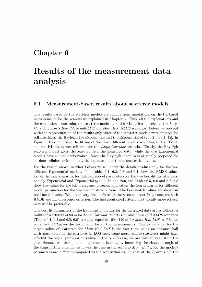
Chapter 6
Results of the measurement dataanalysis
6.1 Measurement-based results about scatterer models
The results based on the scatterer models are coming from simulations on the PL-basedmeasurements for the reasons we explained in Chapter 5. Thus, all the explanations andthe conclusions concerning the scatterer models and the RLL criterion refer to the LargeCorridor, Sports Hall, Main hall LOS and Main Hall NLOS scenarios. Before we proceedwith the representation of the results only three of the scatterer models were suitable forpdf matching, the Rayleigh the Exponential and the Exponential of type 2 model [45]. InFigure 6.1 we represent the fitting of the three different models according to the RMSEand the KL divergence criterion for the Large Corridor scenario. Clearly, the Rayleighscatterer model gives the least fit with the measured data, while the two Exponentialmodels have similar performance. Since the Rayleigh model was originally proposed foroutdoor cellular environments, the explanation of this mismatch is obvious.
For the reason above, in what follows we will show the detailed values only for the twodifferent Exponential models. The Tables 6.1, 6.2, 6.3 and 6.4 show the RMSE valuesfor all the four scenarios, for different model parameters for the two best-fit distributions,namely Exponential and Exponential type 2. In addition, the Tables 6.5, 6.6 and 6.7, 6.8show the values for the KL divergence criterion applied on the four scenarios for differentmodel parameters for the two best fit distributions. The best match values are shown inbold-faced letters. We notice very little differences between the best fit parameters withRMSE and KL divergence criterion. The first mentioned criterion is typically more robust,so it will be preferable.
The best fit parameters of the Exponential models for the measured data are as follows: aradius of scatterers of 80 m for Large Corridor, Sports Hall and Main Hall NLOS scenarios(Tables 6.1, 6.2 and 6.5, 6.6), a radius equal to 100−120 m for Main Hall LOS. A β factorequal to 0.1/R gives the best match for all the measurements. One explanation for thelarger radius of scatterers for Main Hall LOS is the fact that, being an entrance hallwith glass doors at the entrance, in LOS case, some more remote scatterers might haveaffected the signal propagation (while in the NLOS case, we are further away from theglass doors). Another possible explanation is that, by increasing the elevation angle ofthe transmitting antenna, as it was the case in the scenario Main Hall LOS, the model’sparameters are different compared to the rest scenarios. In case of the Sports Hall, the
46

CHAPTER 6. RESULTS OF THE MEASUREMENT DATA ANALYSIS 47
0 10 20 30 40 50 600
0.01
0.02
0.03
0.04
0.05
0.06
0.07
0.08
0.09
[s]
TO
A p
df re
sid
ua
l
KL divergence criterion, Large corridor scenario
ExponentialExponential type 2Rayleigh
0 10 20 30 40 50 600.5
1
1.5
2
2.5
3
3.5
4
4.5x 10
−3
[s]
TO
A p
df
resi
du
al
RMSE criterion, Large corridor scenario
ExponentialExponential type 2Rayleigh
Figure 6.1: Performance of the Rayleigh, Exponential and Exponential type 2 model interms of KL divergence and RMSE criterion, Large Corridor scenario.
RMSE values are slightly higher. The fact that the receiver was always inside the mainbeam of the antenna (i.e., typical LOS condition) is probably less suitable to be modeledby the scatterer models. For the Exponential type 2 model, the best fit values for the σfactor, are between 5 and 7 chips.
Table 6.1: Comparison of Exponential scatterer model in terms of RMSE.
Scenario R=80 m, D=8 m R=100 m, D=10 m R=120 m, D=30 mβ=0.1/R β =0.1/R β =0.1/R
Large Corridor 0.0012 0.0013 0.0015Sports Hall 0.0013 0.0015 0.0018
Main Hall, LOS 0.0016 0.0013 0.0012
Main Hall, NLOS 0.0011 0.0012 0.0015
Table 6.2: Comparison of Exponential scatterer model in terms of RMSE.
Scenario R=80 m, D=8 m R=100 m, D=20 m R=140 m, D=14 mβ =3/R β =1/R β=0.1/R
Large Corridor 0.0429 0.0179 0.0017Sports Hall 0.0424 0.0175 0.0021
Main Hall, LOS 0.0434 0.0187 0.0013Main Hall, NLOS 0.0429 0.0179 0.0017
In the case of Sports Hall and Main Hall LOS scenarios, the Exponential model of type2 gives more accurate results (i.e., lower KL divergence values) than the Exponentialscatterer model, which seems to point out towards the fact that the simple Exponentialmodel of type 2 is more adequate for scenarios with strong LOS components. Last but notleast, it has been observed that the Exponential scatterer model has been independent upto some point of the distance between receiver and transmitter (i.e., distances between 8and 20 m gave similar results, which is explained by the fact that during the measurements,the Tx-Rx distance was varied within this interval).

CHAPTER 6. RESULTS OF THE MEASUREMENT DATA ANALYSIS 48
Table 6.3: Comparison of Exponential of type 2 model in terms of RMSE.
Scenario σ=0.1 chip σ=1 chip σ=5 chips
Large Corridor 0.0587 0.0128 0.0013Sports Hall 0.0582 0.0123 0.0012
Main Hall, LOS 0.0590 0.0136 0.0017Main Hall, NLOS 0.0587 0.0127 0.0011
Table 6.4: Comparison of Exponential of type 2 model in terms of RMSE.
Scenario σ=6 chips σ=7 chips σ=10 chips
Large Corridor 0.0012 0.0013 0.0017Sports Hall 0.0014 0.0016 0.0021
Main Hall, LOS 0.0014 0.0012 0.0013Main Hall, NLOS 0.0011 0.0013 0.0018
Table 6.5: Comparison of Exponential scatterer model in terms of KL divergence.
Scenario R=80 m, D=8 m R=100 m, D=10 m R=120 m, D=30 mβ=0.1/R β =0.1/R β =0.1/R
Large Corridor 0.0077 0.0094 0.0128Sports Hall 0.0067 0.0106 0.0155
Main Hall, LOS 0.0103 0.0071 0.0072Main Hall, NLOS 0.0054 0.0076 0.0113
Table 6.6: Comparison of Exponential scatterer model in terms of KL divergence.
Scenario R=80 m, D=8 m R=100 m, D=20 m R=140 m, D=14 mβ =3/R β =1/R β=0.1/R
Large Corridor 12.3188 1.7148 0.0162Sports Hall 11.9871 1.6339 0.0201
Main Hall, LOS 13.0271 1.8877 0.0083Main Hall, NLOS 12.2322 1.6921 0.0151
Table 6.7: Comparison of Exponential of type 2 model in terms of KL divergence.
Scenario σ=0.1 chip σ=1 chip σ=5 chips
Large Corridor 25.4102 0.8114 0.0083Sports Hall 24.7985 0.7596 0.0062
Main Hall, LOS 26.7161 0.9224 0.0130Main Hall, NLOS 25.2524 0.7961 0.0057
Table 6.8: Comparison of Exponential of type 2 model in terms of KL divergence.
Scenario σ=6 chips σ=7 chips σ=10 chips
Large Corridor 0.0080 0.0098 0.0174Sports Hall 0.0080 0.0113 0.0215
Main Hall, LOS 0.0083 0.0070 0.0088Main Hall, NLOS 0.0059 0.0081 0.0163

CHAPTER 6. RESULTS OF THE MEASUREMENT DATA ANALYSIS 49
6.2 RLL-based multipath characterization
Since the multipath components arrive to the receiver grouped in clusters [20], the abovescenarios were tested also in order to define the number of clusters and multipaths percluster according to the RLL criterion.
The multipath related results are shown in the Tables 6.9 and 6.10. As we can see, allthe four scenarios have a maximum number of clusters equal to 2. We remark that themultipath resolution was limited by the sampling rate (about 16 samples per chip forthe given Fs). The distance between samples (in meters) is therefore about 18.328 m andmultipath components spaced with a separation of less than this value cannot be detected.
Table 6.9: Number of clusters and maximum number of paths to all the four PL-basedscenarios.
Scenario Average number Average number of pathsof clusters per cluster
Large Corridor 1.2569 2.1101Sports Hall 1.2661 1.9174
Main Hall, LOS 1.2905 3.0245Main Hall, NLOS 1.1529 1.6116
Table 6.10: Number of clusters and maximum number of paths to all the four PL-basedscenarios.
Scenario Maximum number of paths Maximum numberper cluster of clusters
Large Corridor 6 2Sports Hall 5 2
Main Hall, LOS 6 2Main Hall, NLOS 5 2
The maximum average number of clusters is met in scenario Main Hall LOS (see Table6.9) which it is in accordance with [15], which states that for large elevation angles theaverage number of clusters is increasing. The scenario Main Hall NLOS has the minimumaverage number of clusters. However, being given the similarities of the measured indoorenvironments, the differences in number of paths and paths per clusters are not large.
6.3 Shadowing/Fading models results
Two scenarios of the PL-based measurements were chosen with two satellite-based mea-surements in order to evaluate the severity of small and large scale fading on them. Bothlarge and small scale fading can be studied together since for Nc = 1 ms we can provide theinformation of the small scale fading and for higher values of Nc up to 5000 ms (the stepwas equal to 100 ms), we can provide the large scale fading information. The extractionof the shadowing information for Nc > 1 ms was based on the method we described inSection 5.2. Thus, in what follows when we mention both small and large scale fading we

CHAPTER 6. RESULTS OF THE MEASUREMENT DATA ANALYSIS 50
refer to: 1 ms ≤ Nc ≤ 5000 ms, while when we mention small scale we refer only to:Nc = 1 ms.
Based on both small and large scale fading, below in the Table 6.11 we show the resultsof the PDF matching for the Large Corridor and the Main Hall NLOS scenarios.
Table 6.11: Distributions fitting for small and large scale fading, based on RMSE and KLdivergence criteria for both scenarios.
Large Corridor Main Hall, NLOSRMSE KL divergence RMSE KL divergence
Rayleigh 0.0355 0.9181 0.0320 0.8266
Nakagami 0.0340 0.8928 0.0321 0.8754Log-normal 0.0330 0.8765 0.0327 0.8790Weibull 0.0362 0.9298 0.0325 0.8449Rice 0.0400 1.1771 0.0323 0.8748GenGamma 0.0330 0.8392 0.0325 0.8449
The parameters for the Generalized Gamma distribution for the Large Corridor scenariowere set to g = 1 and e = 1.4 in order to get the best match. For the Weibull distributionthe value for the βw was set equal to 2.1 (close to Rayleigh distribution). As we can seefrom the table 6.11 both criteria give as best match over the Nc the Generalized Gammadistribution, the RMSE gives also the Log-normal distribution as best match. As wealready discussed the Generalized Gamma distribution is able to model both small andlarge scale fading, the values of the parameters set for e and g are in accordance withthe [28] for LOS environments. The Large Corridor scenario is a LOS environment, forverification see the schematic in Chapter 4. According to the [24] for the same scenariothe best distribution to describe the large scale fading for Nc = 200 ms was the Nakagamidistribution but the comparison was done based on the CDF distributions and for theextraction of the shadowing information it was used only the envelope of the fading signal.
Regarding the Main Hall NLOS scenario the best match distribution is the Rayleigh.That is enhanced also from the fact that the new parameters for the Generalized Gammadistribution of this scenario were set to e=1 and g=2 (Rayleigh case) in order to provideminimum mean value over differentNc (0.0325 according to RMSE criterion). According to[28] in case of NLOS scenario the same parameters for the Generalized Gamma distributionwere tested in order to model both the fast and slow fading. Indeed, the Main HallNLOS scenario is a NLOS scenario and the GPS receiver was seen as shadowed from thetransmitting antenna. For the same scenario the value βw for the Weibull distribution wasset to 2 (Rayleigh case) in order to provide minimum mean value over the Nc. At thispoint it is worth mentioning that based on [40] for the Weibull distribution the severity offading decreases as the βw increases. Thus, in case of the Main Hall NLOS scenario, whereβw is smaller the fading is much more increased compared to the Large Corridor scenario.The above conclusion can be confirmed by the schematic and the receiver’s movement forthe Main Hall NLOS scenario in Chapter 4. In overall, the Figures 6.2 and 6.3 presentdifferent distributions used for both large scale and small scale fading for the two PL-based scenarios. More precisely, the Figures 6.2 and 6.3 show the PDF distributions overdifferent Nc values for the two scenarios.
Concerning the satellite-based measurements both criteria for the Room scenario give theGeneralized Gamma as best distribution, as seen in Table 6.12. The parameters for theGeneralized Gamma distribution were set to g=0.1 and e = 100− 130. Those parameters

CHAPTER 6. RESULTS OF THE MEASUREMENT DATA ANALYSIS 51
0 1000 2000 3000 4000 50000
0.01
0.02
0.03
0.04
0.05
0.06
0.07
Nc [ms]
RM
SE
va
lue
Large Corridor scenario
RayleighNakagami−mLog−normalWeibullRiceGenGamma
0 1000 2000 3000 4000 50000
0.01
0.02
0.03
0.04
0.05
0.06
Nc [ms]
RM
SE
va
lue
Main Hall NLOS scenario
RayleighNakagami−mLog−normalWeibullRiceGenGamma
Figure 6.2: Both fading phenomena over different values of Nc based on the RMSE cri-terion, Left: Large corridor scenario (PL-based). Right: Main Hall NLOS scenario (PL-based).
0 1000 2000 3000 4000 50000
0.5
1
1.5
2
2.5
Nc [ms]
KL
div
erg
en
ce v
alu
e
Large Corridor scenario
RayleighNakagami−mLog−normalWeibullRiceGenGamma
0 1000 2000 3000 4000 50000
0.5
1
1.5
2
Nc [ms]
KL
div
erg
en
ce
va
lue
Main Hall NLOS scenario
RayleighNakagami−mLog−normalWeibullRiceGenGamma
Figure 6.3: Both fading phenomena over different values of Nc based on the KL divergencecriterion, Left: Large corridor scenario (PL-based). Right: Main Hall NLOS scenario (PL-based).

CHAPTER 6. RESULTS OF THE MEASUREMENT DATA ANALYSIS 52
are out of the ranges for LOS or NLOS scenarios based on [28]. The low CNR meanvalues met in this scenario compared to the PL-based scenarios, maybe an explanation forthat. More precisely, CNRwireless = 35.979 dB −Hz for the Room scenario (sat 10) andCNRwireless = 36.132 dB −Hz for the Room scenario (sat 18). The total behaviour ofthe PDF distributions over different Nc values are shown in the Figures 6.4 and 6.5.
Table 6.12: Distributions fitting for small and large scale fading, based on RMSE and KLdivergence criteria for Room scenario.
Room scenario (sat 10) Room scenario (sat 18)RMSE KL divergence RMSE KL divergence
Rayleigh 0.0751 1.6486 0.0687 1.5393Nakagami 0.0771 1.6575 0.0709 1.5556Log-normal 0.0683 1.4292 0.0617 1.3382Weibull 0.0761 1.6631 0.0696 1.5481Rice 0.0833 2.2154 0.0770 2.0835GenGamma 0.0671 1.2505 0.0608 1.1756
0 1000 2000 3000 4000 50000
0.02
0.04
0.06
0.08
0.1
0.12
Nc [ms]
RM
SE
va
lue
Room scenario (sat 10)
RayleighNakagami−mLog−normalWeibullRiceGenGamma
0 1000 2000 3000 4000 50000
0.5
1
1.5
2
2.5
3
Nc [ms]
KL
div
erg
en
ce v
alu
eRoom scenario (sat 10)
RayleighNakagami−mLog−normalWeibullRiceGenGamma
Figure 6.4: Both fading phenomena over different values of Nc for the Room scenario (sat10), Left: Based on the RMSE criterion. Right: Based on the KL divergence criterion.
As we can see in the Figures 6.4 and 6.5 the Rice distribution is far away from the PDF ofthe measurements, according to the two criteria. But in case of the RMSE the Nakagamiand the Weibull distribution show same performance. The parameter βw of the Weibulldistribution reduces to 1.9 providing us the information that in the Room scenario fadingis even more severe compared to the PL-based measurements.
Concerning the small scale fading and keeping the same parameters for the GeneralizedGamma and the Weibull distribution for the different scenarios, we get the following re-sults. Based on the Table 6.13 the multipath fading of the Large Corridor scenario hasWeibull distribution but since the value of the βw is very close to the Rayleigh distributionthen the results for this scenario are in accordance with [24], which states that Rayleighdistribution is the best match for the Large Corridor scenario. For the Main Hall NLOS

CHAPTER 6. RESULTS OF THE MEASUREMENT DATA ANALYSIS 53
0 1000 2000 3000 4000 50000
0.02
0.04
0.06
0.08
0.1
0.12
Nc [ms]
RM
SE
va
lue
Room scenario (sat 18)
RayleighNakagami−mLog−normalWeibullRiceGenGamma
0 1000 2000 3000 4000 50000
0.5
1
1.5
2
2.5
3
Nc [ms]
KL
dive
rgen
ce v
alue
Room scenario (sat 18)
RayleighNakagami−mLog−normalWeibullRiceGenGamma
Figure 6.5: Both fading phenomena over different values of Nc for the Room scenario (sat18), Left: Based on the RMSE criterion. Right: Based on the KL divergence criterion.
0 0.2 0.4 0.6 0.8 10
0.02
0.04
0.06
0.08
0.1
peak amplitude
No
rma
lize
d P
DF
Large Corridor scenario
RayleighNakagami−mLog−normalWeibullRiceGenGammaMeasurements
0 0.2 0.4 0.6 0.80
0.02
0.04
0.06
0.08
0.1
0.12
peak amplitude
No
rma
lize
d P
DF
Main Hall NLOS
RayleighNakagami−mLog−normalWeibullRiceGenGammaMeasurements
Figure 6.6: Normalized PDF for small scale fading (Nc = 1 ms), Left: Large corridorscenario (PL-based). Right: Main Hall NLOS scenario (PL-based).

CHAPTER 6. RESULTS OF THE MEASUREMENT DATA ANALYSIS 54
scenario the best distribution to describe the multipath fading is the Nakagami distri-bution. The m-factor of the Nakagami distribution is equal to 1.07, very close to theRayleigh distribution. Thus, small scale fading in PL-based measurements can be clearlydescribed from the Rayleigh distribution. The PDF of the two scenarios are shown in theFigure 6.6. Finally, based on the satellite measurements the conclusions are almost the
Table 6.13: Distributions fitting for small scale fading, based on RMSE and KL divergencecriteria for both scenarios
Large Corridor Main Hall, NLOSRMSE KL divergence RMSE KL divergence
Rayleigh 0.0034 0.0163 0.0031 0.0041Nakagami 0.0046 0.0146 0.0027 0.0036
Log-normal 0.0103 0.1092 0.0134 0.1300Weibull 0.0033 0.0138 0.0032 0.0040Rice 0.0037 0.0160 0.0032 0.0040GenGamma 0.0205 0.2296 0.0032 0.0040
same as in PL-based measurements. Clearly, the best fit are the Weibull and the Rayleighdistribution for small scale fading. In the Room scenario the Weibull factor βw was setequal to 1.9 which is very close to Rayleigh distribution.
0 0.05 0.1 0.150
0.05
0.1
0.15
0.2
0.25
0.3
0.35
0.4
0.45
peak amplitude
Nor
mal
ized
PD
F
Room scenario (sat 10)
RayleighNakagami−mLog−normalWeibullRiceGenGammaMeasurements
0 0.05 0.1 0.150
0.05
0.1
0.15
0.2
0.25
0.3
0.35
peak amplitude
No
rma
lize
d P
DF
Room scenario (sat 18)
RayleighNakagami−mLog−normalWeibullRiceGenGammaMeasurements
Figure 6.7: Normalized PDF for small scale fading (Nc = 1 ms), Left: Room scenario(sat 10). Right: Room scenario (sat 18).
The CNR mean levels over 1 ms for each scenario are shown in the Figure 6.8. Clearly, theRoom scenario has high levels of noise. That is also an explanation according to [46] whythe Nakagami-m distribution cannot provide good matching with the small scale fadingfor the Room scenario. The m factor of the Nakagami-m distribution is coming from thecomputation of the mean and the variance of the wireless signal (see Section 3.2), whichin the presence of noise its computation might be inaccurate.

CHAPTER 6. RESULTS OF THE MEASUREMENT DATA ANALYSIS 55
Table 6.14: Distributions fitting for small scale fading, based on RMSE and KL divergencecriteria for Room scenario
Room scenario (sat 10) Room scenario (sat 18)RMSE KL divergence RMSE KL divergence
Rayleigh 0.0052 0.0248 0.0045 0.0191
Nakagami 0.0543 0.3685 0.0537 0.3709Log-normal 0.0176 0.0514 0.0184 0.0591Weibull 0.0032 0.0235 0.0035 0.0193Rice 0.0102 0.0342 0.0091 0.0279GenGamma 0.0704 0.5428 0.0503 0.3348
0 1 2 3 4 5 6
x 104
30
35
40
45
50
55
60
Time [ms]
CN
R [d
B−
Hz]
Main Hall NLOS scenariomean(Ref. Cable) = [56.913 45.042] dB
ReferenceIndoor
0 1 2 3 4 5 6
x 104
30
35
40
45
50
55
60
Time [ms]
CN
R [
dB
−H
z]
Large Coridor scenariomean(Ref. Indoor) = [56.861 46.498] dB
ReferenceIndoor
0 1 2 3 4 5 6
x 104
10
15
20
25
30
35
40
45
50
Time [ms]
CN
R [d
B−
Hz]
Room scenario (sat 10)mean(Ref. Indoor) = [39.795 35.979] dB
ReferenceIndoor
0 1 2 3 4 5 6
x 104
5
10
15
20
25
30
35
40
45
50
Time [ms]
CN
R [d
BH
z]
Room scenario (sat 18)mean(Ref. Cable)= [42.446 36.132] dB
ReferenceIndoor
Figure 6.8: CNR mean values for both the reference and the wireless signal for all the fourscenarios.

CHAPTER 6. RESULTS OF THE MEASUREMENT DATA ANALYSIS 56
6.4 I/Q-based multipath detection results
As we already discussed in Chapter 5, the purpose of this work is to draw some preliminaryconclusions (since the investigation based on the carrier phase is new in itself) and setsome first thresholds. Variables such as the CNR, the path spacing in case of multipathscenarios, the power levels of the multipath components, and the type of the PRN usedfor autocorrelation are going to be tested and see the effect of those on the area plottedfrom the imaginary versus the real component of the correlator output. Concerning thepath spacing, the type of the PRN used for autocorrelation and the power levels of themultipath components, there is still much research to be done and it is left for future work.
In case of the PRN code it can either be a BPSK-modulated real code (denoted as PRNreal) or a BPSK-modulated complex code (denoted as PRN complex). The frequency usedfor the carrier is equal to 1575.42 MHz and the spreading factor was set equal to 1023.The idea here is to create the circumstances that the signal may face to a real situationand see the effects on the area plotted from the imaginary versus the real component.For that reason we generated in matlab a GPS signal passing through a static channel(time invariant channel) and a Rayleigh channel (time variant channel). The correlatoroutput of the distorted signal with the local PRN code is used for investigation. Basically,two main scenarios were created with two subscenarios each based on the multipath profileused for investigation. The two main scenarios are characterized from the type of the PRNcode used: PRN real and PRN complex. Those two scenarios were tested for two differentmultipath profiles. The first multipath profile was characterized by multipath componentsof power levels equal to: 0 dB, -1 dB, -2 dB and -3 dB (denoted as 1 dB multipath profile),including the 1-path, 2-path, 3-path and 4-path multipath scenarios respectively. Thefirst arriving component is always assumed stronger than the rest three. For the secondmultipath profile the power levels of the multipath components were assumed to be: 0dB, -3 dB, -6 dB and -9 dB (denoted as 3 dB multipath profile), where the next arrivingsignal is half power of the previous one. The CNR were set from 20-120 dB-Hz whileboth scenarios were tested under a fading and a static channel. The conclusions will bebased on the calculated area plotted from the imaginary versus the real component ofthe correlator output for both the static and the fading channel. Apart from the areacomposed from the imaginary and the real component, the normalized area was computedas well. The normalized area is plotted from the imaginary versus the real component overthe maximum value
√
I2 +Q2. An example of the calculated area and the normalizedarea for both static and fading channels is shown in the Figures 6.9 and 6.10. For thisexample, the CNR was set to 80 dB-Hz, the path spacing is equal to 1 chip delay andthe 1 dB multipath profile was used for the assumed 3-path scenario. In the Figure 6.9 wecan see the area coming from the imaginary versus the real component of the correlatoroutput for the fading and the static channel when the PRN code used is real. On the otherhand, in the Figure 6.10 we can see the area coming from the imaginary versus the realcomponent of the correlator output for the fading and the static channel when the PRNcode used is complex.
In the same way, in the Figure 6.11 we show the results for the calculated area and thenormalized area when we plot the imaginary versus the real component of the correlatoroutput, for both fading and static channels. The total number of points used for eachmultipath scenario and for each CNR value was equal to 200, while the evaluated areais coming as the mean value over the 200 random points. The results are based on theassumption that the local code was PRN real. Moreover, it was assumed 1 dB multipathprofile and the path spacing between consecutive paths was set equal to 1 chip delay. As

CHAPTER 6. RESULTS OF THE MEASUREMENT DATA ANALYSIS 57
we can see, in case of the fading channel there can be a threshold that can show us thepresence of one multipath component. The choice of the threshold was done empiricallybased on the upper plots of the Figure 6.11. More precisely, the value of the thresholdfor the results based on the area only, was set equal to 0.02 and in case of the normalizedarea the threshold value was set equal to 0.05. For the static channel we could not setany threshold to show us the presence of one multipath component according to the lowerplots of the Figure 6.11.
Keeping the path spacing constant and the multipath profile the same we shifted from thereal to the complex BPSK modulated PRN. The same procedure was repeated concerningthe computations of the areas coming from both static and fading channels. The samethresholds we defined even in case where the PRN complex was used. The related plots forboth static and fading channels are shown in the Figure 6.12. Different values of CNR upto 120 dB-Hz were also tested in order to verify the fact that the noise level does not haveany effect on the total performance of the two channels for different multipath scenarios.
−0.2 0 0.2 0.4 0.6−0.2
0
0.2I/Q diagram, Fading channel
I
Q
−0.5 0 0.5 1 1.5 2−0.5
0
0.5I/Q normalized diagram, Fading channel
I normal.
Q n
orm
al.
−0.5 0 0.5 1 1.5 2 2.5−5
0
5x 10
−3 I/Q diagram, Static channel
I
Q
−0.1 0 0.1 0.2 0.3 0.4 0.5 0.6−1
0
1x 10
−3 I/Q normalized diagram, Static channel
I normal.
Q n
orm
al.
Figure 6.9: Examples of the area and the normalized area for both static and fadingchannels (1 dB multipath profile, PRN real, path spacing:1 chip delay, 3-path scenario,CNR:80 dB-Hz).
Since we saw the results of the areas computations for both static and fading channels incase of 1 dB multipath profile, it is time to provide the same plots for the 3 dB multipathprofile. Keeping the path spacing the same and equal to 1 chip delay we got the resultsbased on the area computations for both fading and static channels for either PRN realor complex. The information for the different scenarios is shown in the Figures 6.13 and6.14. According to the plots of the Figures 6.13 and 6.14, we noticed that in case of the 3dB multipath profile the threshold value can be kept the same as before in order to providethe information for the presence of more than one multipath component in multipathscenarios. The same observation we can make when the PRN complex code is used, seeFigures 6.13 and 6.14 again. For the static channel even in case where the power levelsof the multipath components differ half power to each other it is still difficult to define athreshold that can show us the presence of one multipath component. At this point wehave to mention that we did not present the plots based on the normalized area since theydo not provide any further useful information.
If we increase the path spacing between consecutive multipath components from 1 chipdelay to 3 chips delay and keep the 3 dB multipath profile the same, we get the plots of the

CHAPTER 6. RESULTS OF THE MEASUREMENT DATA ANALYSIS 58
−0.2 0 0.2 0.4 0.6 0.8 1 1.2−0.5
0
0.5
1I/Q diagram, Fading channel
I
Q
−0.2 0 0.2 0.4 0.6 0.8 1 1.2−0.5
0
0.5
1I/Q normalized diagram, Fading channel
I normal.
Q n
orm
al.
−0.5 0 0.5 1 1.5−0.02
0
0.02I/Q diagram, Static channel
I
Q
−0.1 0 0.1 0.2 0.3 0.4 0.5 0.6 0.7−0.01
0
0.01I/Q normalized diagram, Static channel
I normal.
Q n
orm
al.
Figure 6.10: Examples of the area and the normalized area for both static and fadingchannels (1 dB multipath profile, PRN complex, path spacing:1 chip delay, 3-path scenario,CNR:80 dB-Hz).
Figure 6.15. Based on the results of the Figure 6.15 we can see that the initial thresholdvalue should be reduced in order to estimate correctly the presence of more than one pathsin multipath scenarios. As we can observe when the path spacing increases, the computedvalues for the area are getting smaller for the multipath scenarios. To the same conclusionwe come up even when the PRN complex code is used, see Figure 6.15. Thus, regardlessthe type of the PRN code used, in order to be able to provide reliable results for thepresence of more than one paths in case of multipath scenarios with the use of the initialthreshold values, the path spacing between consecutive multipath components should bekept minimum. For the static channel even when we increased the path spacing from 1chip delay to 3 chips delay, we could not set any threshold to provide us the informationfor the presence of more than one multipath components in case of multipath scenarios.The conclusion is the same either we are based on the results coming from the area’s orthe normalized area’s computations.
Following on, after we defined the thresholds for the presence of one multipath component,we next proceeded with the verification of those thresholds. For that reason we generateddifferent correlator outputs under fading multipath channel and we applied the thresholdswe set based on the area’s and the normalized area’s results. More precisely, in case of1-path scenario the calculated area should be less or less equal than 0.02 (the thresholdvalue). In case of 2-path scenario the calculated area should be greater than 0.02 in orderto provide correct results. The same conditions were applied also in case of the 3-pathscenario and the 4-path scenario. In the same way we proceeded with the threshold basedon the normalized area for the four different multipath scenarios. The success of theresults will be expressed in percentage, in total there were 800 random points (200 foreach multipath scenario).
Based on the Figure 6.16 we can see the effect of the path spacing in case of 1 dB multipathprofile. As we already noticed, in case the path spacing increases between consecutive pathsthe ability to predict correctly the presence of one path in multipath scenarios fails. Thefailure is even greater for the 3 dB multipath profile, see Figure 6.17. Thus, in case the 3chips delay is used as path spacing, the ability to predict correctly the presence of morethan one path in case of multipath scenarios fails more when the consecutive components

CHAPTER 6. RESULTS OF THE MEASUREMENT DATA ANALYSIS 59
1 1.5 2 2.5 3 3.5 40
0.02
0.04
0.06
0.08
0.1
0.12
0.14
0.16
0.18
paths
am
plitu
de
Fading Channel (PRN real)I/Q area based, 1dB multipath profile, path spacing=1 chips delay
CNR=20 dB−HzCNR=40 dB−HzCNR=60 dB−HzCNR=80 dB−HzCNR=100 dB−HzCNR=120 dB−Hz
1 1.5 2 2.5 3 3.5 40
0.05
0.1
0.15
0.2
0.25
0.3
0.35
0.4
paths
am
plitu
de
Fading Channel (PRN real)I/Q normal. area based, 1 dB multipath profile, path spacing=1 chip delay
CNR=20 dB−HzCNR=40 dB−HzCNR=60 dB−HzCNR=80 dB−HzCNR=100 dB−HzCNR=120 dB−Hz
1 1.5 2 2.5 3 3.5 40.4
0.6
0.8
1
1.2
1.4
1.6
1.8
2
2.2
2.4x 10
−5
paths
am
plitu
de
Static Channel, (PRN real)I/Q area based, 1 dB multipath profile, path spacing=1 chip delay
CNR=20 dB−HzCNR=40 dB−HzCNR=60 dB−HzCNR=80 dB−HzCNR=100 dB−HzCNR=120 dB−Hz
1 1.5 2 2.5 3 3.5 45
5.5
6
6.5
7
7.5
8x 10
−6
paths
am
plitu
de
Static Channel, (PRN real)I/Q normalized area based, 1 dB multipath profile, path spacing=1 chip delay
CNR=20 dB−HzCNR=40 dB−HzCNR=60 dB−HzCNR=80 dB−HzCNR=100 dB−HzCNR=120 dB−Hz
Figure 6.11: Area and normalized area results for different CNR values, Upper plots:Fading multipath channel. Lower plots: Static multipath channel.(1 dB multipath profile,PRN real, path spacing:1 chip delay)

CHAPTER 6. RESULTS OF THE MEASUREMENT DATA ANALYSIS 60
1 1.5 2 2.5 3 3.5 40
0.02
0.04
0.06
0.08
0.1
0.12
0.14
0.16
0.18
paths
am
plitu
de
Fading Channel, PRN complexI/Q area based, 1 dB multipath profile, path spacing=1 chip delay
CNR=20 dB−HzCNR=40 dB−HzCNR=60 dB−HzCNR=80 dB−HzCNR=100 dB−HzCNR=120 dB−Hz
1 1.5 2 2.5 3 3.5 40
0.05
0.1
0.15
0.2
0.25
0.3
0.35
paths
am
plitu
de
Fading Channel, PRN complexI/Q normal. area based, 1 dB multipath profile, path spacing= 1chip delay
CNR=20 dB−HzCNR=40 dB−HzCNR=60 dB−HzCNR=80 dB−HzCNR=100 dB−HzCNR=120 dB−Hz
1 1.5 2 2.5 3 3.5 40.005
0.01
0.015
0.02
0.025
0.03
paths
am
plitu
de
Static Channel, PRN complexI/Q area based, 1 dB multipath profile, path spacing=1 chip delay
CNR=20 dB−HzCNR=40 dB−HzCNR=60 dB−HzCNR=80 dB−HzCNR=100 dB−HzCNR=120 dB−Hz
1 1.5 2 2.5 3 3.5 45
5.5
6
6.5
7
7.5
8
8.5
9
9.5
10x 10
−3
paths
am
plitu
de
Static Channel, PRN complexI/Q normal. area based, 1 dB multipath profile, path spacing= 1 chip delay
CNR=20 dB−HzCNR=40 dB−HzCNR=60 dB−HzCNR=80 dB−HzCNR=100 dB−HzCNR=120 dB−Hz
Figure 6.12: Area and normalized area results for different CNR values, Upper plots:Fading multipath channel. Lower plots: Static multipath channel.(1 dB multipath profile,PRN complex, path spacing:1 chip delay)
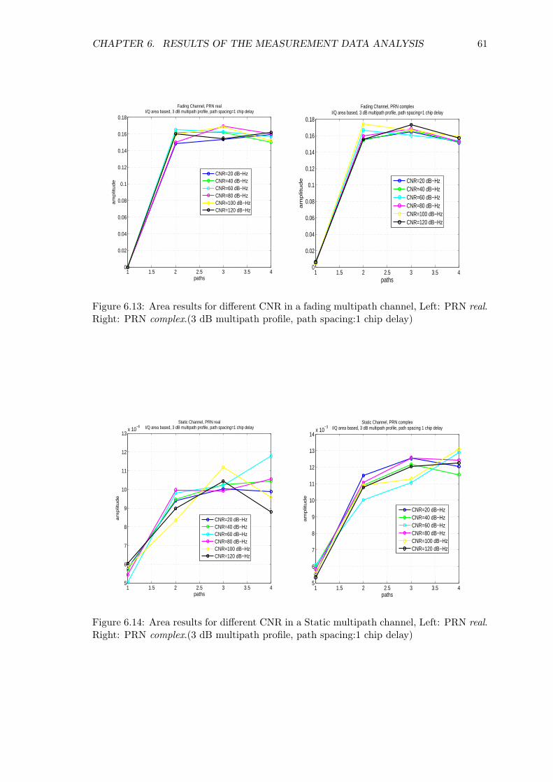
CHAPTER 6. RESULTS OF THE MEASUREMENT DATA ANALYSIS 61
1 1.5 2 2.5 3 3.5 40
0.02
0.04
0.06
0.08
0.1
0.12
0.14
0.16
0.18
paths
am
plit
ud
e
Fading Channel, PRN realI/Q area based, 3 dB multipath profile, path spacing=1 chip delay
CNR=20 dB−HzCNR=40 dB−HzCNR=60 dB−HzCNR=80 dB−HzCNR=100 dB−HzCNR=120 dB−Hz
1 1.5 2 2.5 3 3.5 40
0.02
0.04
0.06
0.08
0.1
0.12
0.14
0.16
0.18
paths
am
plitu
de
Fading Channel, PRN complexI/Q area based, 3 dB multipath profile, path spacing=1 chip delay
CNR=20 dB−HzCNR=40 dB−HzCNR=60 dB−HzCNR=80 dB−HzCNR=100 dB−HzCNR=120 dB−Hz
Figure 6.13: Area results for different CNR in a fading multipath channel, Left: PRN real.Right: PRN complex.(3 dB multipath profile, path spacing:1 chip delay)
1 1.5 2 2.5 3 3.5 45
6
7
8
9
10
11
12
13x 10
−6
paths
am
plit
ud
e
Static Channel, PRN realI/Q area based, 3 dB multipath profile, path spacing=1 chip delay
CNR=20 dB−HzCNR=40 dB−HzCNR=60 dB−HzCNR=80 dB−HzCNR=100 dB−HzCNR=120 dB−Hz
1 1.5 2 2.5 3 3.5 45
6
7
8
9
10
11
12
13
14x 10
−3
paths
am
plit
ud
e
Static Channel, PRN complexI/Q area based, 3 dB multipath profile, path spacing 1 chip delay
CNR=20 dB−HzCNR=40 dB−HzCNR=60 dB−HzCNR=80 dB−HzCNR=100 dB−HzCNR=120 dB−Hz
Figure 6.14: Area results for different CNR in a Static multipath channel, Left: PRN real.Right: PRN complex.(3 dB multipath profile, path spacing:1 chip delay)

CHAPTER 6. RESULTS OF THE MEASUREMENT DATA ANALYSIS 62
1 1.5 2 2.5 3 3.5 40
0.01
0.02
0.03
0.04
0.05
0.06
0.07
0.08
0.09
paths
am
plit
ud
e
Fading Channel,PRN realI/Q area based, 3 dB multipath profile, path spacing 3 chips delay
CNR=20 dB−HzCNR=40 dB−HzCNR=60 dB−HzCNR=80 dB−HzCNR=100 dB−HzCNR=120 dB−Hz
1 1.5 2 2.5 3 3.5 40
0.01
0.02
0.03
0.04
0.05
0.06
0.07
0.08
0.09
paths
am
plit
ud
e
Fading Channel, PRN complexI/Q area based, 3 dB multipath profile, path spacing= 3 chips delay
CNR=20 dB−HzCNR=40 dB−HzCNR=60 dB−HzCNR=80 dB−HzCNR=100 dB−HzCNR=120 dB−Hz
Figure 6.15: Area results for different CNR in a Fading multipath channel (3 dB multipathprofile, path spacing:3 chips delay), Left: PRN real. Right: PRN complex.
differ more in power. This latter conclusion concerns the results based on the normalizedarea.
20 40 60 80 100 12091
91.5
92
92.5
93
93.5
94
94.5
95
95.5
CNR [dB−Hz]
% s
ucce
ss
Fading Channel, PRN real1 dB multipath profile, path spacing=1 chip delay
based on I/Q area thresholdbased on I/Q normalized area threshold
20 40 60 80 100 12070
70.5
71
71.5
72
72.5
73
73.5
74
74.5
75
CNR [dB−Hz]
% s
ucce
ss
Fading Channel, PRN real1 dB multipath profile, path spacing= 3 chips delay
based on the I/Q area thresholdbased on the I/Q normalized area threshold
Figure 6.16: Percentage of success based on area and normalized area threshold for differentCNR values (PRN real, 1 dB multipath profile), Left: Path spacing:1 chip delay. Right:Path spacing:3 chips delay.
In overall, from the results based on the fading channel we saw that we can set empiricalthresholds able to describe the presence of more than one paths in multipath scenarios. Incase of the static channel we could not set any threshold either based on the area’s or thenormalized area’s computations of the correlator output. Thus, the following conclusionsare valid for the fading channel only:
• Based on the path spacing, we saw that keeping the path spacing minimum between

CHAPTER 6. RESULTS OF THE MEASUREMENT DATA ANALYSIS 63
20 40 60 80 100 12091
91.5
92
92.5
93
93.5
94
94.5
95
95.5
96
CNR [dB−Hz]
% s
ucce
ss
Fading Channel, PRN real3 dB multipath profile, path spacing 1 chip delay
based on I/Q area thresholdbased on I/Q normalized area threshold
20 40 60 80 100 12066
67
68
69
70
71
72
73
74
75
CNR [dB−Hz]
% s
ucce
ss
Fading Channel, PRN real3 dB multipath profile, path spacing 3 chips delay
based on I/Q area thresholdBased on I/Q normalized area threshold
Figure 6.17: Percentage of success based on area and normalized area threshold for differentCNR values (PRN real, 3 dB multipath rpofile), Left: Path spacing:1 chip delay. Right:Path spacing:3 chips delay.
consecutive paths we can provide more reliable results for the presence of more thanone paths in multipath scenarios.
• Based on the power levels of the consecutive paths when the path spacing increases,the success to predict correclty the presence of more than one path in multipathscenarios is getting worse when the power levels differ more.
• The PRN code used (either real or complex BPSK modulated) did not provide dif-ferent results.
• Regardless the path spacing and the power levels of the consecutive multipath com-ponents, the results based on the area are more reliable compared to the normalizedarea’s results. This is valid for all the CNR values we used in the simulations.

Chapter 7
Conclusions and future work
The conclusions of the thesis work and the contributions to the multipath identificationconcerning GPS signals and possible future research topics are presented in this Chapter.Basically the conclusions and the future work will be based on the four main issues thatthis work tried to investigate: scatterer models applied for indoor GPS signals, identifica-tion of total number of clusters and number of multipath components per cluster for GPSindoor environments based on the RLL criterion, small scale and large scale fading charac-terization for GPS signals for both indoor and outdoor environments, and I/Q area-basedmultipath detection.
7.1 Conclusions
Regarding the scatterer models, the Exponential distribution scatterer model was able todescribe the pdf of TOA for indoor PL-based scenarios. The factors that the Exponentialscatterer model took into account were: the distance between the transmitter and thereceiver, the radius of the cell and a factor β dependent of the under-test type of environ-ment. The Exponential scatterer model was proposed for indoor environments and indeedit was able to model the pdf of TOA for all the four PL-based indoor environments. Forall the four scenarios, the radius of the assumed cell was 80-100 m and the β factor equalto 0.1 over that radius. Any small change on the distance between the transmitter andthe receiver did not provide much difference to the results. Apart from the Exponentialscatterer model, we also tested a simple Exponential model (denoted as Exponential modelof type 2 in Chapter 3) dependent of only the σD factor. The σD factor was valued as 5-7chips delay for the four PL-based scenarios. The Elliptical scatterer model, although itwas applicable for indoor environments, in our case it could not provide any match withthe measured pdf of TOA. That was because the model took into account a maximumtime delay τm, see Chapter 3 again. In case of indoor environments the appropriate valuesfor the maximum time delay, as they were found in the literature, was in terms of ns butfor our measurements the maximum time delay was in terms of µs. The high noise levelsto the correlator output may be an explanation for that.
The RLL criterion based on the correlator output of the incoming signal with the local PRNcode was tested to identify the number of clusters and the number of paths per cluster forPL-based indoor environments. Even though the model did not take into account closelyspaced multipaths, we identified 2 clusters for all the four scenarios and 2-3 paths percluster. Moreover, we observed the effect of the elevation angle on the average number of
64

CHAPTER 7. CONCLUSIONS AND FUTURE WORK 65
clusters in case of the Main Hall scenario. The results of our measurements were limitedto identify enough paths even though the delay resolution (Ts = 61 ns) provided by thesampling rate (Fs = 16.36 MHz) used in our measurements was good enough.
Regarding the large scale fading, we presented a modified way to extract the large scalefading information based on the power of the incoming fading envelope for different coher-ent integration lengths. Based on the modified method to evaluate the large scale fadinginformation we managed to encompass both small and large scale fading in order to applythe Generalized Gamma, the Rice, the Rayleigh, the Nakagami-m, the Log-normal andthe Weibull distribution. As it was expected, in case of both small and large scale fading,the Generalized Gamma distribution provided best match. The parameters used for theGeneralized Gamma distribution for our measurements in case of LOS and NLOS, werein accordance with the values found in the literature. More precisely, for the Main HallNLOS scenario the appropriate parameters for the Generalized Gamma distribution were:e = 1 and g = 2. On the other hand, for the Large Corridor scenario the values for theGeneralized Gamma distribution were equal to: e = 1.4 and g = 1. Concerning the smallscale fading the Weibull and the Rayleigh distributions performed really good to describethe pdf of the measurements for both PL-based and satellite-based scenarios. In accor-dance with that were also the results of earlier studies for the same PL-based scenariosconcerning the fit of the Rayleigh distribution. The Nakagami-m distribution in case ofsatellite-based scenarios did not provide good match since the noise level was higher thanthe rest PL-based scenarios.
Finally, concerning the observation of the distorted LOS correlation peak due to multipath.Based on the method we described in Chapter 5, we tried to detect the multipath effectbased on the area plotted from the real versus the imaginary component of the correlatoroutput. Modeling both static and fading channels, in case of the static channel we couldnot set any threshold to provide the presence of more than one path in multipath scenarios.The PRN code used (either real or complex BPSK modulated) did not provide differentresults. Concerning the path spacing between consecutive paths, we saw that keeping thepath spacing minimum we could provide more reliable results for the presence or not ofmore than one path for multipath scenarios. Last but not least, regardless of the pathspacing and the power levels of the consecutive multipath components, the results basedon the area were more reliable even for small CNR values.
7.2 Future work
Based on the statistical distributions results and the modified method proposed to encom-pass both small and large scale fading, the performance of the combined distributions thatthey were proposed in [23] for different lengths of Nc could be further tested . Moreover,since the Generalized Gamma distribution did not provide best match to the satellite-based data, or at least the parameters we found for e and g were out of the ranges for LOSand NLOS scenarios. The satellite-based measurements could be tested for parametersapplied in case of NLOS environments with smaller Nc values.
In this thesis the scatterer models and the RLL criterion were applied only for PL-basedmeasurements in indoor environments due to the low CNR found in the satellite-basedscenarios. Based on new measurement data with higher CNR values, both in satellite andPL environments, other scatterer models can be tested and evaluated. Due to the geom-etry of the satellite-based measurements, the models that assume local scatterers around

CHAPTER 7. CONCLUSIONS AND FUTURE WORK 66
the receiver may be more reliable to provide the correct pdf of TOA. Recommendablescatterer models for that, are the ROS scatterer model, the DOS scatterer model and theCircular scatterer model. All the three just mentioned scatterer models are applicable tomacrocellular environments and they assume that the scatterers are located in an areaaround the receiver.
Finally, based on the I/Q area-based multipath detection study, a better way to improvethe evaluation of the plotted area can provide us better thresholds concerning the presenceof one, two, three or even four paths in multipath scenarios. Till now we could identifythe presence of more than one path in multipath scenarios without being able to providethe accurate number of them. Moreover, based on the factors able to affect the results ofthe area’s computations or the normalized area’s computations we could study further thefollowing parameters:
• The effect of the path spacing between consecutive multipath components. Theconclusions till now concerning the path spacing are based either for 1 chip delay or3 chips delay.
• The effect of the coherent integration length (Nc). In the present work the coherentintegration length was constant and equal to 10 ms.
• The power levels of the multipath components providing different values betweenconsecutive paths, excluding the 1 dB multipath profile and the 3 dB multipath profile.
• The Multiplexed Binary Offset Carrier (MBOC) modulated PRN code could betested and evaluated in case of fading and static channels.
Last but not least, based on the measurements the evaluation of the area plotted fromthe imaginary versus the real component of the correlator output in case of PL-basedand satellite-based scenarios could be compared and discussed with the RLL results (forPL-based measurements).
Bibliography
[1] G. W. Hein, J. A. Avila Rodriguez, S. Wallner, B. Eissfeller, T. Pany, and P. Hartl.Envisioning a future GNSS system of systems, Part 1. InsideGNSS, pages 58–67,January/February 2007.
[2] Smithsonian National Air and Space Museum. http://www.nasm.si.edu/gps. [Ac-cessed January 2009].
[3] G. Pistoia. Battery operated devices and systems. Elsevier publications, 2008.
[4] B. Eissfeller, G. Ameres, V. Kropp, and D. Sanroma. Performance of GPS, GLONASSand Galileo. Eissfeller et al., pages 185–199, 2007.
[5] Sidereus 2008. COMPASS satellite navigation system development. China satellitenavigation project center, November 2008.
[6] S. Dong, H. Wu, X. Li, S. Guo, and Q. Yang. The Compass and its time referencesystem. BIPM and IOP Publishing LTd, pages 47–50, December 2008.
[7] A. Dempster. QZSS’s Indoor Messaging System, GNSS Friend or Foe? Inside GNSS,pages 37–40, January/February 2009.
[8] N. Salama. Global Positioning, Technologies and Performance. Wiley and Sons Inc.,April 2008.
[9] European Space Agency (ESA). http://www.esa.int/. [Accessed January 2009].
[10] Naviva a business unit of Space Systems Finland (SSF) Oy.http://www.naviva.fi/pseudolites/. [Accessed February 2009].
[11] H. S. Cobb. GPS Pseudolites: Theory Design and Applications. Ph.D. dissertation,Stanford University California, September 1997.
[12] V. Badea and R. Eriksson. Indoor Navigation with Pseudolites. Master Thesis,University of Linkoping Sweden, January 2005.
[13] L. Dai, J. Wang, T. Tsujii, and C. Rizos. Pseudolite-based inverted positioning andits applications. 5 th Int. Symp. on Satellite Navigation Technology and Applications,pages 24–27, 2001.
[14] Federal Communications Commission. http://www.fcc.gov/pshs/services/911-services. Public safety and Homeland security bureau, [Accessed January 2009].
[15] G. Hein, M. Paonni, V. Kropp, and A. Teuber. GNSS Indoors Fighting the Fadingpart 1. Inside GNSS, pages 43–52, March/April 2008.
67

BIBLIOGRAPHY 68
[16] M. Sahmoudi and R. Jr. Landry. Multiptath Mitigation Techniques Using Maximum-Likelihood Principle. Inside GNSS, pages 24–29, November/December 2008.
[17] R. Ertel and J. Reed. Angle and Time of Arrival Statistics for Circular and EllipticalScattering Models. Selected Areas in Communications, 17(11):1829–1840, November1999.
[18] L. Jiang and S. Y. Tan. Geometrically Based Statistical Channel Models for Out-door and Indoor Propagation Environments. Transactions on Vehicular Technology,56(6):3587–3593, November 2007.
[19] S. Al-Jazzar, J. Caffery, and H. R. You. A Scattering Model Based Approach to NLOSMitigation in TOA Location Systems. IEEE Vehicular Technology Conference, 2002.
[20] A. Saleh and R. Valenzuela. A Statistical Model for Indoor Multipath Propagation.Selected Areas in Communications, SAc-5:128–137, February 1987.
[21] A. Lakhzouri, E. S. Lohan, I. Saastamoinen, and M. Renfors. Interference and Indoorchannel Propagation Modeling Based on GPS Satellite Signal Measurements. In Proc.of ION-GPS, September 2005.
[22] J. R. A. Watson. High-Sensitivity GPS L1 Signal Analysis for Indoor Channel Mod-eling. Master Thesis, University of Calgary Kanada, April 2005.
[23] A. K. M. Najmul Islam. CNR Estimation and Indoor Channel Modeling of GPSSignals. Master Thesis, Tampere University of Technology Finland, March 2008.
[24] A. K. M. Islam, E. Lohan, A. Lahkouri, E. Pajala, H. Laitinen, and M. Renfors.Indoor fading distributions for GPS-based pseudolite signals. IEEE Satellite andSpace Communications, 2007.
[25] O. Mubarak and A. Dempster. Carrier phase analysis to mitigate multipath effect.IGNSS symposium, December 2007.
[26] P. Taaghol and R. Tafazolli. Correlation model for shadow fading in landmobilesatellite systems. IEEE Electronics Letters, 33(15):1287–1289, July 1997.
[27] A. J. Coulson, A. G. Williamson, and R.G Vaughan. Improved fading distributionfor mobile radio. IEEE Proc. Commun., 145(3):197–202, June 1998.
[28] S. Wyne, A. F. Molisch, P. Almers, G. Eriksson, J. Karedal, and F. Tufvesson. Sta-tistical Evaluation of Outdour-to-Indoor Office MIMO Measurements at 5.2GHz. inVTC 2005, pages 146–150, 2005.
[29] B. Sklar. Rayleigh Fading Channels in Mobile Digital Communications Systems, PartI:Characterization. IEEE Communications Magazine, pages 90–100, July 1997.
[30] T. S. Rappaport. Wireless Communications, Principles and Practice. Prentice Hall,2002.
[31] T. S. Sarkar. Smart Antennas. Willey Series in Microwave and Optical Engineering,2003.
[32] A. Alighanbari and C. D. Sarris. High Order S-MRTD Time-Domain Modeling ofFading, Characteristics of wireless channels. IEEE Antennas and Propagation SocietyInternational Symposium, 2006.

BIBLIOGRAPHY 69
[33] S. Al-Jazzar, J. Caffery, and H. You. Scattering-Model-Based methods for TOALocation in NLOS Environments. Transactions on Vehicular Technology, 56(2):583–593, March 2007.
[34] P. Petrus, J. Reed, and T. Rappaport. Geometrical-based statistical macrocell chan-nel model for mobile environments. IEEE Transactions on Vehicular Technology,50(3):495–502, March 2002.
[35] R. Janaswamy. Angle and time of arrival statistics for the Gaussian scatter densitymodel. IEEE Transactions on Wireless Commun., 1(3):488–497, July 2002.
[36] S. Mahhoud, Z. Hussain, and P. O’Shea. Geometrical model for mobile radio channelwith hyperbolically distributed scatterers. Proc. ICCS, 1:17–20, November 2002.
[37] J. C. Liberti and T. S. Rappaport. A geometrically based model for line-of-sightmultipath radio channels. in Proc. IEEE Vehicular Technology Conf., pages 844–848,April 1996.
[38] Bensty, Sondi, and Huang. Handbook of speech processing. Springer, 2008.
[39] J. Proakis. Digital Communications. McGraw-Hill New York USA, 1995.
[40] N. Sagias, D. Zogas, G. Karagiannidis, and G. Tombras. Channel Capacity andSecond-Order Statistics in Weibull Fading . IEEE Communications letters, pages377–379, June 2004.
[41] M. K. Simon and M. S. Alouini. Digital Communication over Fading Channels. Wileyseries in Telecommunications and Signal Processing, 2000.
[42] A. Lahkouri, E. Lohan, I. Saastamoinen, and M. Renfors. On Second Order Statisticsof the Satellite-to-Indoor channel Based on Field Measurements. IEEE 16th Interna-tional Symposium on Personal, Indoor and Mobile Radio Communications, 2005.
[43] M. Gudmundson. Correlation model for shadow fading in mobile radio systems. IEEEElectronics Letters, 27(23):2145–2146, November 1991.
[44] Bensty, Sondi, and Huang. Handbook of speech processing. Springer, 2008.
[45] A. Kalaitzi and E. S. Lohan. Multipath Characterization via Scatterer Models andReturn-to-low Level Concept for Pseudolite Indoor Channels. ESA Workshop Ra-diowave Propagation Models, Tools and Data for Space Systems, 3-5 December 2008.
[46] A. Lakhzouri, E. S. Lohan, I. Saastamoinen, and M. Renfors. Measurement andCharacterization of Satellite-to-Indoor Radio Wave Propagtion Channel. ENC-GNSS,July 2005.