ants & eigenanatomy - brainmapping.org · imaging (dti), and decreases in cortical thickness,...
TRANSCRIPT

ANTs & Eigenanatomy
Brian Avants Penn Image Computing and Sciences LaboratoryUniversity of Pennsylvania, Philadelphia, PA.
July 18, 2013
Joint work with PICSL, Ben Kandel, Lyle Ungar, Paramveer Dhillon, M. Farah, M.Grossman, H Hurt, J Kim & many more
Wednesday, July 17, 13

Wednesday, July 17, 13

My work: Medical imaging analytics to produce scientifically/clinically relevant
measurements from difficult data.
Wednesday, July 17, 13

My work: Medical imaging analytics to produce scientifically/clinically relevant
measurements from difficult data.
... large data sets,
Wednesday, July 17, 13

My work: Medical imaging analytics to produce scientifically/clinically relevant
measurements from difficult data.
... large data sets,babies,
Wednesday, July 17, 13

My work: Medical imaging analytics to produce scientifically/clinically relevant
measurements from difficult data.
... large data sets,babies,stroke,
Wednesday, July 17, 13

My work: Medical imaging analytics to produce scientifically/clinically relevant
measurements from difficult data.
... large data sets,babies,stroke,
brain injury,
Wednesday, July 17, 13
My work: Medical imaging analytics to produce scientifically/clinically relevant
measurements from difficult data.
... large data sets,babies,stroke,
brain injury,severe neurodegeneration ...
Wednesday, July 17, 13

Brain Registration @ UPENN
We developed Advanced Normalization Tools (ANTs) to improve imaging science and healthcare through open source mathematical software. We contribute to this & other software to improve standardization & reproducibility.
We use ANTs to study (often basic) questions about (a) the human lifespan, (b) evolution, (c) pharmaceutical intervention, (d) longitudinal change and structural/functional network relationships with (e) cognition, (f) disease and (g) normal variation in the environment.
We also promote open science.
History: Implementation
Thompson 1917Horn 1980
Gee 1994
Bajcsy 1988
Miller 1996 Guimond 1999 Ashburner 2000
(PICSL) ANTsMM 7 / 56
White matter and thickness atrophy rates significantly correlated ( p < 0.009, permutation).
Volume to Disc (or square)
InSANE
12 months6 months1 month
Code set at x-1
Code set at x+1Code set at x
7
7
ARTICLES
Corey T. McMillan, PhDBrian Avants, PhDDavid J. Irwin, MDJon B. Toledo, MDDavid A. Wolk, MDVivianna M. Van Deerlin,
MD, PhDLeslie M. Shaw, PhDJohn Q. Trojanoswki,
MD, PhDMurray Grossman, MD,
EdD
Correspondence toDr. McMillan:[email protected]
Editorial, page 126
Supplemental data atwww.neurology.org
Supplemental Data
Can MRI screen for CSF biomarkers inneurodegenerative disease?
ABSTRACT
Objective: Alzheimer disease (AD) and frontotemporal lobar degeneration (FTLD) may have over-lapping clinical presentations despite distinct underlying neuropathologies, thus making in vivodiagnosis challenging. In this study, we evaluate the utility of MRI as a noninvasive screening pro-cedure for the differential diagnosis of AD and FTLD.
Methods: We recruited 185 patients with a clinically diagnosed neurodegenerative disease con-sistent with AD or FTLDwho had a lumbar puncture and a volumetric MRI. A subset of 32 patientshad genetic or autopsy-confirmed AD or FTLD. We used singular value decomposition to decom-pose MRI volumes and linear regression and cross-validation to predict CSF total tau (tt) andb-amyloid (Ab1-42) ratio (tt/Ab) in patients with AD and patients with FTLD. We then evaluatedaccuracy of MRI-based predicted tt/Ab using 4 converging sources including neuroanatomicvisualization and categorization of a subset of patients with genetic or autopsy-confirmed ADor FTLD.
Results: Regression analyses showed that MRI-predicted tt/Ab is highly related to actual CSFtt/Ab. In each group, both predicted and actual CSF tt/Ab have extensively overlapping neuro-anatomic correlates: low tt/Ab consistent with FTLD is related to ventromedial prefrontal regionswhile high tt/Ab consistent with AD is related to posterior cortical regions. MRI-predicted tt/Ab is75% accurate at identifying underlying diagnosis in patients with known pathology and in clini-cally diagnosed patients with known CSF tt/Ab levels.
Conclusion: MRI may serve as a noninvasive procedure that can screen for AD and FTLD pathol-ogy as a surrogate for CSF biomarkers. Neurology! 2013;80:132–138
GLOSSARYAb 5 b-amyloid; AD 5 Alzheimer disease; FTLD 5 frontotemporal lobar degeneration; GM 5 gray matter; ROI 5 region ofinterest; SVD 5 singular value decomposition; tt 5 total tau.
There is urgent need to improve in vivo diagnosis of neurodegenerative conditions like Alzheimerdisease (AD) and frontotemporal lobar degeneration (FTLD) because of potential treatments target-ing the underlying abnormal proteinopathies. Despite distinct biochemical abnormalities, AD andFTLD often share similar clinical features and thus clinical diagnosis alone is unreliable.1 CSFbiomarkers based on a ratio of total tau (tt) and b-amyloid (Ab1-42) (tt/Ab) provide a highlysensitive and specific in vivo diagnostic tool for discriminating between AD and FTLD.2–4 In ourautopsy series, tt/Ab yields 90% sensitivity and 97% specificity.4 Despite reasonable diagnosticaccuracy, a lumbar puncture is often viewed by patients as invasive. In the setting of a clinical trialwhere repeated monitoring of endpoints such as CSF biomarkers may be important, an alternativebiomarker that provides equivalent diagnostic accuracy, but is more appealing to patients, would beideal. Volumetric MRI may serve this role since patients with autopsy- or CSF-defined AD andFTLD have relatively distinct neuroanatomic profiles of gray matter (GM) neurodegeneration.5–7
We present a novel screening method for discriminating between AD and FTLD based onMRI-predicted tt/Ab CSF values in individuals. This approach yields a single, biologically
From the Department of Neurology (C.T.M., D.J.I., D.A.W., M.G.), Center for Neurodegenerative Disease Research (D.J.I., J.B.T., V.M.V.D.,L.M.S., J.Q.T.), Department of Radiology (B.A.), Penn Memory Center (D.A.W.), and Department of Pathology & Laboratory Medicine (V.M.V.D., L.M.S., J.Q.T.), University of Pennsylvania, Philadelphia.
Go to Neurology.org for full disclosures. Funding information and disclosures deemed relevant by the authors, if any, are provided at the end of thearticle.
132 © 2013 American Academy of Neurology
ª 2013 American Academy of Neurology. Unauthorized reproduction of this article is prohibited.
Symmetric di!eomorphic image registration withcross-correlation: Evaluating automated labeling
of elderly and neurodegenerative brain
B.B. Avants a,*, C.L. Epstein b, M. Grossman c, J.C. Gee a
a Department of Radiology, University of Pennsylvania, 3600 Market Street, Philadelphia, PA 19104, United Statesb Department of Mathematics, University of Pennsylvania, Philadelphia, PA 19104, United States
c Department of Neurology, University of Pennsylvania, Philadelphia, PA 19104, United States
Received 11 November 2006; received in revised form 23 May 2007; accepted 6 June 2007Available online 23 June 2007
Abstract
One of the most challenging problems in modern neuroimaging is detailed characterization of neurodegeneration. Quantifying spatialand longitudinal atrophy patterns is an important component of this process. These spatiotemporal signals will aid in discriminatingbetween related diseases, such as frontotemporal dementia (FTD) and Alzheimer’s disease (AD), which manifest themselves in the sameat-risk population. Here, we develop a novel symmetric image normalization method (SyN) for maximizing the cross-correlation withinthe space of di!eomorphic maps and provide the Euler–Lagrange equations necessary for this optimization. We then turn to a carefulevaluation of our method. Our evaluation uses gold standard, human cortical segmentation to contrast SyN’s performance with a relatedelastic method and with the standard ITK implementation of Thirion’s Demons algorithm. The new method compares favorably withboth approaches, in particular when the distance between the template brain and the target brain is large. We then report the correlationof volumes gained by algorithmic cortical labelings of FTD and control subjects with those gained by the manual rater. This comparisonshows that, of the three methods tested, SyN’s volume measurements are the most strongly correlated with volume measurements gainedby expert labeling. This study indicates that SyN, with cross-correlation, is a reliable method for normalizing and making anatomicalmeasurements in volumetric MRI of patients and at-risk elderly individuals.Published by Elsevier B.V.
Keywords: Di!eomorphic; Deformable image registration; Human cortex; Dementia; Morphometry; Cross-correlation
1. Introduction
Frontotemporal dementia (FTD) prevalence may behigher than previously thought and may rival Alzheimer’sdisease (AD) in individuals younger than 65 years (Ratnav-alli et al., 2002). Because FTD can be challenging to detectclinically, it is important to identify an objective method tosupport a clinical diagnosis. MRI studies of individualpatients are di"cult to interpret because of the wide rangeof acceptable, age-related atrophy in an older cohort sus-ceptible to dementia. This has prompted MRI studies that
look at both the rate and the anatomic distribution ofchange (Chan et al., 2001; Fox et al., 2001; Studholmeet al., 2004; Kertesz et al., 2004; Avants et al., 2005a; Ball-maier et al., 2004).
Manual, expert delineation of image structures enablesin vivo quantification of focal disease e!ects and serves asthe basis for important studies of neurodegeneration (Stud-holme et al., 2004). Expert structural measurements fromimages also provide the gold-standard of anatomical eval-uation. The manual approach remains, however, severelylimited by the complexity of labeling 2563 or more voxels.Such labor is both time consuming and expensive to sup-port, while the number of individual experts available forsuch tasks is limited. A third significant di"culty is the
1361-8415/$ - see front matter Published by Elsevier B.V.doi:10.1016/j.media.2007.06.004
* Corresponding author.E-mail address: [email protected] (B.B. Avants).
www.elsevier.com/locate/media
Available online at www.sciencedirect.com
Medical Image Analysis 12 (2008) 26–41
Dementia induces correlated reductions in white matter integrity andcortical thickness: A multivariate neuroimaging study with sparsecanonical correlation analysis
Brian B. Avants a,⁎, Philip A. Cook a, Lyle Ungar b, James C. Gee a, Murray Grossman c
a Penn Image Computing and Science Laboratory, Department of Radiology, University of Pennsylvania, Philadelphia, PA 19104-6389, USAb Penn Image Computing and Science Laboratory, Department of Computer Science, University of Pennsylvania, Philadelphia, PA 19104-6389, USAc Penn Image Computing and Science Laboratory, Department of Neurology, University of Pennsylvania, Philadelphia, PA 19104-6389, USA
a b s t r a c ta r t i c l e i n f o
Article history:Received 6 October 2009Revised 6 January 2010Accepted 12 January 2010Available online 18 January 2010
Key words:DementiaMultivariateCorrelationDiffusion tensorCortical thicknessADFTDCanonical correlation
We use a new, unsupervised multivariate imaging and analysis strategy to identify related patterns ofreduced white matter integrity, measured with the fractional anisotropy (FA) derived from diffusion tensorimaging (DTI), and decreases in cortical thickness, measured by high resolution T1-weighted imaging, inAlzheimer's disease (AD) and frontotemporal dementia (FTD). This process is based on a novelcomputational model derived from sparse canonical correlation analysis (SCCA) that allows us toautomatically identify mutually predictive, distributed neuroanatomical regions from different imagingmodalities. We apply the SCCA model to a dataset that includes 23 control subjects that are demographicallymatched to 49 subjects with autopsy or CSF-biomarker-diagnosed AD (n=24) and FTD (n=25) with bothDTI and T1-weighted structural imaging. SCCA shows that the FTD-related frontal and temporal degenerationpattern is correlated across modalities with permutation corrected pb0.0005. In AD, we find significantassociation between cortical thinning and reduction in white matter integrity within a distributed parietaland temporal network (pb0.0005). Furthermore, we show that—within SCCA identified regions—significantdifferences exist between FTD and AD cortical-connective degeneration patterns. We validate these distinct,multimodal imaging patterns by showing unique relationships with cognitive measures in AD and FTD. Weconclude that SCCA is a potentially valuable approach in image analysis that can be applied productively todistinguishing between neurodegenerative conditions.
© 2010 Elsevier Inc. All rights reserved.
Introduction
Neuroimaging studies suggest that frontotemporal dementia(FTD) leads to decreases in cortical thickness and white matterintegrity, and these may reflect degraded cortical and white matterneural networks underlying language, social and executive function-ing. Alzheimer's disease (AD) also induces large-scale neurodegen-eration that, in contrast to FTD, may reflect episodic memory loss.However, the distinguishing, integrated effects of these diseases onthe cortical and white matter networks underlying these behavioralchanges have not been established.
FTD is an early-onset neurodegenerative condition with anaverage age of onset in the sixth decade of life (Hodges et al.,2003; Neary and Snowden, 1996; Grossman, 2006). The disease isdue to a disorder of tau metabolism (Lee et al., 2001) or theaccumulation of a ubiquinated protein known as TDP-43 (Neumannet al., 2006). The condition is almost as common as AD in individuals
less than 65 years of age (Rosso et al., 2003; Knopman et al., 2004;Cairns et al., 2006). Survival is typically 8 years from onset (Hodgeset al., 2003; Cairns et al., 2006; Xie et al., 2008). Developing bio-markers for early detection of disease and assessment of treatment isof great significance because of the development of therapiesspecifically for this condition.
One common, inexpensive, non-invasive tool in diagnosis of FTD isclinical measurement of cognitive abilities and behavior. Diagnosis ofFTD consequently includes observation of syndromes such as primaryprogressive aphasia (PPA) and/or a disorder of social comportmentand personality together with limited executive resources (McKhannet al., 2001; Neary et al., 1998). Recent studies have begun todemonstrate longitudinal decline on language and cognitivemeasuresin clinical (Blair et al., 2007; Libon et al., 2009b) and pathologicallydefined (Grossman et al., 2008) populations. However, whenvalidated against autopsy defined series, clinical diagnostic assess-ment may be inaccurate in up to 30% of cases (Forman et al., 2006).Most of the missed diagnoses are uncommon, young-onset presenta-tions of AD. Thus, comparative studies of patients with neurodegen-erative conditions are needed to demonstrate the specificity of amethod for accurate diagnosis.
NeuroImage 50 (2010) 1004–1016
⁎ Corresponding author.E-mail address: [email protected] (B.B. Avants).
1053-8119/$ – see front matter © 2010 Elsevier Inc. All rights reserved.doi:10.1016/j.neuroimage.2010.01.041
Contents lists available at ScienceDirect
NeuroImage
j ourna l homepage: www.e lsev ie r.com/ locate /yn img
Geodesic estimation for large deformation anatomical shapeaveraging and interpolation
Brian Avants and James C. Gee*
University of Pennsylvania, Philadelphia, PA 19104, United States
Available online 11 September 2004
The goal of this research is to promote variational methods for
anatomical averaging that operate within the space of the underlying
image registration problem. This approach is effective when using the
large deformation viscous framework, where linear averaging is not
valid, or in the elastic case. The theory behind this novel atlas building
algorithm is similar to the traditional pairwise registration problem,
but with single image forces replaced by average forces. These group
forces drive an average transport ordinary differential equation
allowing one to estimate the geodesic that moves an image toward
the mean shape configuration. This model gives large deformation
atlases that are optimal with respect to the shape manifold as defined
by the data and the image registration assumptions. We use the
techniques in the large deformation context here, but they also pertain
to small deformation atlas construction. Furthermore, a natural,
inherently inverse consistent image registration is gained for free, as
is a tool for constant arc length geodesic shape interpolation. The
geodesic atlas creation algorithm is quantitatively compared to the
Euclidean anatomical average to elucidate the need for optimized
atlases. The procedures generate improved average representations of
highly variable anatomy from distinct populations.
D 2004 Elsevier Inc. All rights reserved.
Keywords: Atlas creation; Nonrigid image registration; Inverse consistent;
Geodesic averaging; Morphometry
Introduction
Anatomical atlases have tremendous value in today’s medicalenvironment where large databases are mined for diagnostic,research, and pedagogical information. High-resolution atlases are
an instance of anatomy upon which teaching or surgical planningis based (Kikinis et al., 1996; Miller et al., 1993; Yelnik et al.,2003). Surgical procedures may employ atlas-based image
registration for planning the placement of deep-brain stimulators(Dawant et al., 2003). Average anatomical atlases provide a least-biased coordinate system for surgical planning, functional local-
ization studies (Ashburner and Friston, 1996), or for studyingstructure–function relationships (Letovsky et al., 1998). They alsooperate as a reference frame for understanding the normal
variation of anatomy (Talairach and Tournoux, 1988) and as aprobabilistic space into which functional or structural features aremapped (Le Briquer and Gee, 1997). Genomics researchers
currently build atlases to investigate the relationship of genotypeto phenotype (Mackenzie-Graham et al., 2004), which is a majorfocus of the Allen Brain Institute (Allen Brain Atlas). Perform-ance of algorithms based on manipulating empirical information,
such as active shape (Cootes et al., 1995), should also benefitfrom use of an average model.
Computerized atlases based on magnetic resonance (MR)
images may compile either average shape (Le Briquer and Gee,1997), average intensity, or both (Guimond et al., 2000) within asingle image. The Euclidean shape space, shown in Fig. 1, is often
assumed for these models leading to the use of linear averaging ofthe transformations and intensity to produce the atlases. Deviationsfrom the mean shape or intensity may then be captured separately
by statistical models such as principal components (Cootes et al.,1995; Le Briquer and Gee, 1997). Average intensities aretraditionally found by first computing transformations from ananatomical instance to a population data set. The averages of these
displacement fields, which take a member of the population to theremainder of the data, represent an average in the sense ofanatomical positions. This average transformation must then be
inverted to gain the average shape (Guimond et al., 2000).However, positional differences are not explicitly minimized inthe registration problem, typically because one promotes smooth-
ness by using differential measures in the face of ill-posedproblems (Tikhonov and Arsenin, 1977).
One difficulty with this approach is that the process ofaveraging transformations may destroy the optimal properties of
the individual transformations. For example, the average of largedeformation displacement fields, each of which satisfies theminimization of a well-defined variational energy, may no longer
1053-8119/$ - see front matter D 2004 Elsevier Inc. All rights reserved.
doi:10.1016/j.neuroimage.2004.07.010
* Corresponding author. University of Pennsylvania, 3600 Market
Street, Suite 370, Philadelphia, PA 19104. Fax: +1 619 349 8552.
E-mail addresses: [email protected] (B. Avants)[email protected] (J.C. Gee).
Available online on ScienceDirect (www.sciencedirect.com.)
www.elsevier.com/locate/ynimg
NeuroImage 23 (2004) S139–S150
Lagrangian frame di!eomorphic image registration:Morphometric comparison of human and chimpanzee cortex
Brian B. Avants *, P. Thomas Schoenemann, James C. Gee
Departments of Bioengineering, Radiology and Anthropology, University of Pennsylvania, Philadelphia, PA 19104-6389, United States
Received 30 September 2004; received in revised form 9 February 2005; accepted 4 March 2005Available online 3 June 2005
Abstract
We develop a novel Lagrangian reference frame di!eomorphic image and landmark registration method. The algorithm uses thefixed Langrangian reference frame to define the map between coordinate systems, but also generates and stores the inverse map fromthe Eulerian to the Lagrangian frame. Computing both maps allows facile computation of both Eulerian and Langrangian quan-tities. We apply this algorithm to estimating a putative evolutionary change of coordinates between a population of chimpanzee andhuman cortices. Inter-species functional homologues fix the map explicitly, where they are known, while image similarities guide thealignment elsewhere. This map allows detailed study of the volumetric change between chimp and human cortex. Instead of basingthe inter-species study on a single species atlas, we di!eomorphically connect the mean shape and intensity templates for each group.The human statistics then map di!eomorphically into the space of the chimpanzee cortex providing a comparison between species.The population statistics show a significant doubling of the relative prefrontal lobe size in humans, as compared to chimpanzees.! 2005 Elsevier B.V. All rights reserved.
Keywords: Di!eomorphic; Deformable image registration; Primate cortex; Evolution; Morphometry
1. Introduction
The relationship between the primate and the humanbrain has intrigued researchers in evolution, biology andmedicine since at least the 19th century (Huxley et al.,1874; Thompson, 1917) and remains an area of active re-search (Deacon, 1997; Schoenemann et al., 2004; Essen,2004a). Understanding functional and anatomical inter-species correspondences is fundamental to connectinghuman and animal research. Chimpanzee language, dis-ease and behavioral studies are often used as a startingpoint for understanding human medical conditions.These studies become more valuable as our ability to re-late them to human subjects increases. Volumetric med-ical image registration permits one to make inter-speciesneuroanatomical comparisons between subjects by using
known functional and structural constraints. Further-more, di!eomorphic transformations (Miller et al.,2002) between species (Essen et al., 2001) may aid inunderstanding the evolutionary process.
Di!eomorphisms permit comparisons under thehypothesis that the topology of the deforming anatomymust be preserved. Transformations are di!erentiableand guaranteed to be one-to-one and onto: for every po-sition in one image, there is a single corresponding posi-tion in the second image. These properties also meanthat the transformations may be composed. If we havea transformation taking I to J and a transformation tak-ing J to K, we also have both I to K and K to I throughcomposition. The di!eomorphic framework also sup-plies a rigorous mathematical metric between anato-mies, a valuable quantitative measure of the distancebetween images.
Landmarking is an invaluable tool for gaining ana-tomically correct image registrations in cases where
1361-8415/$ - see front matter ! 2005 Elsevier B.V. All rights reserved.doi:10.1016/j.media.2005.03.005
* Corresponding author.E-mail address: [email protected] (B.B. Avants).
www.elsevier.com/locate/media
Medical Image Analysis 10 (2006) 397–412
Characterization of sexual dimorphism in the human corpus callosumAbraham Dubb,* Ruben Gur,1 Brian Avants,2 and James Gee3
Departments of Bioengineering, Psychiatry, and Radiology, University of Pennsylvania, Philadelphia, PA 19104-6389, USA
Received 11 December 2002; revised 2 May 2003; accepted 8 May 2003
Abstract
Despite decades of research, there is still no agreement over the presence of gender-based morphologic differences in the human corpuscallosum. We approached the problem using a highly precise computational technique for shape comparison. Starting with a prospectivelyacquired sample of cranial MRIs of healthy volunteers (age ranges 18–84), the variations of individual callosa are quantified with respectto a reference callosum shape in the form of Jacobian determinant maps derived from the geometric transformations that map the referencecallosum into anatomic alignment with the subject callosa. Voxelwise t tests performed over the determinant values demonstrated thatfemales had a larger splenium than males (P ! 0.001 uncorrected for multiple comparisons) while males possessed a larger genu (P !0.001). In addition, pointwise Pearson plots using age as a correlate showed a different pattern of age-related changes in male and femalecallosa, with female splenia tending to expand more with age, while the male genu tended to contract. Our results demonstrate significantmorphologic differences in the corpus callosum between genders and a possible sex difference in the neuro-developmental cycle.© 2003 Elsevier Inc. All rights reserved.
1. Introduction
Differences in higher cortical functioning between malesand females have been the target of considerable investiga-tion for a number of decades. Cognitive and functionalimaging studies have suggested a greater degree of hemi-spheric lateralization in males compared to females, whilefemales displayed increased bilateral hemispheric activityfor a variety of cognitive tasks (Harshman and Remington,1976; McGlone, 1980; Bryden, 1979; Kimura and Harsh-man, 1984; Shaywitz et al., 1995). These studies seem tosuggest enhanced interhemispheric communication in fe-males and have motivated investigation into sexual dimor-phism of the corpus callosum. The corpus callosum is thebrain’s largest white-matter tract and the primary means ofcommunication between the two cerebral hemispheres,prompting investigators to hypothesize that differences incallosal size exist between males and females. Most inves-tigators have examined the shape and size of the mid-
sagittal section of the callosum as a surrogate for the struc-ture’s overall shape. To date, however, no consensus hasbeen reached on the presence of such gender-based differ-ences in the callosum. De Lacoste and Holloway (1982)reported in 1982 that the female splenium was more bulbousthan the tubual male splenium. Follow-up studies by DeLacoste et al. (1986), Yoshi et al. (1986), and Allen et al.(1991) all found increased size in the female splenium. Incontrast, Weis and colleagues (Weis et al., 1989), Going andDixson (1990), and Witelson (1985) all reported no suchdifferences between the callosa of males and females.
One possible reason for this prevailing controversy maybe the lack of standards in callosal analysis. While cross-sectional area and callosal length are the more traditionalindices reported in gender studies, there is little agreementover how to normalize these indices. Furthermore, grossdimensional measures will miss regional shape variations incallosa. Some investigators have divided the callosa intopartitions and compared the area of corresponding partitionsbetween study groups (Witelson, 1985). The difficulty hereis that the selection of the partitioning method is arbitraryand subpartition size differences may escape detection.
We used template deformation morphometry (TDM)(Machado and Gee, 1998; Machado et al., 2000; Davatzikos
* Corresponding author.E-mail address: [email protected] (A. Dubb).1 E-mail address: [email protected] (R. Gur).2 E-mail address: [email protected] (B. Avants).3 E-mail address: [email protected] (J. Gee).
NeuroImage 20 (2003) 512–519 www.elsevier.com/locate/ynimg
1053-8119/03/$ – see front matter © 2003 Elsevier Inc. All rights reserved.doi:10.1016/S1053-8119(03)00313-6
Generating Template Functional Connectivity Networks via
Prior Based Eigenanatomy
June 19, 2013
Abstract
We present a new framework for prior-constrained sparse decomposition of matrices derivedfrom neuroimaging data and apply this method to functional network analysis of a clinicallyrelevant population. Matrix decomposition methods are powerful dimensionality reductiontools that can aid interpretability of large-scale datasets. However, the unconstrained natureof the optimization algorithms may make it di�cult to interpret results in a specific applicationdomain. For instance, approaches like Group Independent Component Analysis (ICA) requirepost-hoc methods to derive subject specific networks and to identify the anatomical associationof the derived independent components. ICA approaches also average subject specific networkcharacteristics and may be di�cult to interpret at an individual level or in terms of the graph-based metrics that have recently gained popularity in fMRI analysis. The traditional seedROI-based approach to deriving networks from BOLD fMRI overcomes these problems but hasshortcomings of its own. Seed-based approaches may “over-average” within a region and maybe sensitive to ROI placement, co-registration errors and the specific ROI boundaries.
In this paper, we propose a novel approach which integrates ideas from the matrix decom-position and the ROI paradigms. We formulate our novel solution in terms of prior-constrained`1 penalized (sparse) principal component analysis. Like ICA, our approach seeks to identifya data-driven matrix decomposition of a matrix. However, our approach, Prior Based Eige-nanatomy (p-Eigen), also constrains the individual components by a spatial anatomical prior.Consequently, p-Eigen leads to statistically refined definitions of ROIs based on local covari-ance structure of the data matrix. p-Eigen provides a principled way of incorporating priorinformation in the form of probabilistic or binary ROIs while still allowing the data to softlymodify the original ROI definitions.
When applied to functional neuroimaging data, this allows us to construct subject specificnetworks with reduced sensitivity to ROI placement. We evaluate our method within a classi-fication paradigm. We show that p-Eigen graph metrics significantly aid classification of earlyMild Cognitive Impairment (MCI) as well as prediction of Delayed Recall when compared tometrics derived from standard registration-based ROI definitions, totally data driven ROIs anda model based on standard demographics plus hippocampal volume. Our results also revealunique relationship between default mode network (DMN) and hippocampus network structureand psychometric measurements of memory.
1 Introduction and Related Work
The presence of large and diverse neuroimaging datasets has brought the importance of data analysistechniques into focus. These issues are particularly salient in BOLD fMRI where recent papers
1
Neuroinformatics for Genome-Wide 3D GeneExpression Mapping in the Mouse Brain
Lydia Ng, Sayan D. Pathak, Chihchau Kuan, Christopher Lau, Hongwei Dong,Andrew Sodt, Chinh Dang, Brian Avants, Paul Yushkevich, James C. Gee,
David Haynor, Ed Lein, Allan Jones, and Mike Hawrylycz
Abstract—Large-scale gene expression studies in the mammalian brain offer the promise of understanding the topology, networks,and, ultimately, the function of its complex anatomy, opening previously unexplored avenues in neuroscience. High-throughput
methods permit genome-wide searches to discover genes that are uniquely expressed in brain circuits and regions that controlbehavior. Previous gene expression mapping studies in model organisms have employed in situ hybridization (ISH), a technique that
uses labeled nucleic acid probes to bind to specific mRNA transcripts in tissue sections. A key requirement for this effort is thedevelopment of fast and robust algorithms for anatomically mapping and quantifying gene expression for ISH. We describe a
neuroinformatics pipeline for automatically mapping expression profiles of ISH data and its use to produce the first genomic scale3D mapping of gene expression in a mammalian brain. The pipeline is fully automated and adaptable to other organisms and tissues.
Our automated study of more than 20,000 genes indicates that at least 78.8 percent are expressed at some level in the adult C56BL/6Jmouse brain. In addition to providing a platform for genomic scale search, high-resolution images and visualization tools for expression
analysis are available at the Allen Brain Atlas web site (http://www.brain-map.org).
Index Terms—Bioinformatics (genome or protein) databases, data mining, registration, segmentation, information visualization.
Ç
1 INTRODUCTION
SEVERAL high-throughput efforts are underway to system-atically analyze gene expression patterns in the mam-
malian central nervous system (CNS) [1], [2], [3]. Theseprojects strive to gain insight into temporal and spatialexpression of specific genes throughout CNS developmentand in the adult brain. Advances in genomic sequencingmethods, high-throughput technology [4], [5], [6], [7], andbioinformatics through robust image processing [8], [9] nowenable the neuroscience community to study nervoussystem function at the genomic scale. Central to theseneuro-genomics efforts is understanding gene transcriptionin the context of the spatial anatomy and connectivity of thenervous system [10].
Of the several techniques presently available for explor-ing large-scale gene expression [1], [11], [12], in situhybridization (ISH) is one of the most compelling becauseof its ability to study the anatomic localization of specific
gene expression in the brain [13]. Perhaps more so than
other currently available biotechnologies, ISH offers the
promise of cellular level specificity and microstructural
identification, two major interests of modern neurobiology.
However, in order to localize expression patterns in the
brain, it is critical to establish a universal coordinate system
and a compatible anatomic ontology for the brain, ideally
with multiple hierarchical levels, and methods of data
presentation that facilitate comparison of the expression
patterns of multiple genes [14], [15].The Allen Brain Atlas (ABA) informatics pipeline
addresses the challenge of automating the mapping of
3D gene expression patterns on a genomic scale. The
primary goal of the pipeline is to acquire and process data
on the expression of individual genes in a fashion that will
enable online anatomic structural search, visualization, and
data mining of ISH imagery. A secondary goal is to develop
tools to facilitate visual and computational discovery. In
this paper, we describe the ABA informatics platform and
methodology and some of the publicly available tools and
illustrate the power of the method via genomic level pattern
searches.The ABA informatics automated pipeline, illustrated in
Fig. 1, consists of modules supporting the following
functions:
. image preprocessing, including tile stitching anddirect compression into JPEG2000 format,
. image storage and indexing,
. access to a novel online digital reference atlas for theadult C56Bl/6J mouse brain [16],
382 IEEE/ACM TRANSACTIONS ON COMPUTATIONAL BIOLOGY AND BIOINFORMATICS, VOL. 4, NO. 3, JULY-SEPTEMBER 2007
. L. Ng, S.D. Pathak, C. Kuan, C. Lau, H. Dong, A. Sodt, C. Dang, E. Lein,A. Jones, and M. Hawrylycz are with the Allen Institute for Brain Science,551 North 34th Street, Suite 200, Seattle, WA 98103.E-mail: {lydian, sayanp, leonardk, chrisl, hongweid, andrews, chinhda, edl,allanj, mikeh}@alleninstitute.org.
. B. Avants, P. Yuskevich, and J. Gee are with the Department of Radiology,University of Pennsylvania, 3600 Market Street, Suite 370, Philadelphia,PA 19104-2644.E-mail: [email protected], [email protected],[email protected].
. D. Haynor is with the Department of Radiology, University ofWashington, Box 356004, Seattle, WA 98195-6004.E-mail: [email protected].
Manuscript received 21 Mar. 2006; revised 30 June 2006; accepted 10 Sept.2006; published online 12 Jan. 2007.For information on obtaining reprints of this article, please send e-mail to:[email protected], and reference IEEECS Log Number TCBB-0083-0306.Digital Object Identifier no. 10.1109/TCBB.2007.1035.
1545-5963/07/$25.00 ! 2007 IEEE Published by the IEEE CS, CI, and EMB Societies & the ACM
Behavioral/Cognitive
Regional and Hemispheric Variation in Cortical Thickness inChimpanzees (Pan troglodytes)
William D. Hopkins1,2 and Brian B. Avants3
1Division on of Developmental and Cognitive Neuroscience, Yerkes National Primate Research Center, Atlanta, Georgia 30322, 2Neuroscience Institute andLanguage Research Center, Georgia State University, Atlanta, Georgia 30302, and 3Department of Radiology, University of Pennsylvania, Philadelphia,Pennsylvania 19104-6389
Recent advances in structural magnetic resonance imaging technology and analysis now allows for accurate in vivo measurement ofcortical thickness, an important aspect of cortical organization that has historically only been conducted on postmortem brains. In thisstudy, for the first time, we examined regional and lateralized cortical thickness in a sample of 71 chimpanzees for comparison withpreviously reported findings in humans. We also measured gray and white matter volumes for each subject. The results indicated thatchimpanzees showed significant regional variation in cortical thickness with lower values in primary motor and sensory cortex comparedwith association cortex. Furthermore, chimpanzees showed significant rightward asymmetries in cortical thickness for a number ofregions of interest throughout the cortex and leftward asymmetries in white but not gray matter volume. We also found that total andregion-specific cortical thickness was significantly negatively correlated with white matter volume. Thus, chimpanzees with greater whitematter volumes had thinner cortical thickness. The collective findings are discussed within the context of previous findings in humansand theories on the evolution of cortical organization and lateralization in primates.
IntroductionIn modern structural brain imaging protocols, cortical volume(CV) is a main measure of interest from the standpoint of under-standing disease progression, development, and aging. CV ismade up of cortical thickness, surface area, and the white matter(WM) that underlies connectivity between regions. In terms ofbrain evolution, the human brain is approximately three timeslarger than that of chimpanzees, the closest living relative tohumans (Rilling and Insel, 1999b; Semendeferi and Damasio,2000; Semendeferi et al., 2001; Schoenemann, 2006; Sherwoodet al., 2012). In addition, humans have disproportionateincreases in gray and particularly white matter volume com-pared with other primates (Rilling and Insel, 1999a;Schoenemann et al., 2005; Rogers et al., 2010). It has beensuggested that the relative increase in white matter volumeand gyrification are prominent in brain regions, such as theprefrontal cortex (PFC) and temporal lobes, that are thoughtto underlie certain human cognitive specializations (Deacon,1997; Semendeferi et al., 1998; Rilling and Seligman, 2002;Roth and Dicke, 2005; Schoenemann et al., 2005).
An important aspect of cortical organization that has not beenexamined from a comparative primate perspective is corticalthickness. Studies of postmortem human brains have shown thatthere are significant regional and lateralized differences in corti-cal thickness. For instance, in postmortem material, corticalthickness varies from !2– 4 mm across the human cerebrum,with thinner cortex found in primary motor and sensory regionscompared with thicker cortex in association cortex (Rabinowiczet al., 1999). Recent advances in in vivo imaging technologies usedwith human brains have largely validated these findings (Luderset al., 2006b), when derived from T1-weighted structural mag-netic resonance imaging (MRI) scans (Luders et al., 2006b). Interms of lateralization, small but significant asymmetries in cor-tical thickness have been found in the human brain includingleftward biases for the precentral gyrus (PreCG), middle frontal,anterior temporal, and superior parietal lobes (SPLs). Significantrightward biases have been reported for inferior posterior tem-poral lobe and inferior frontal gyrus (IFG) (Luders et al., 2006a)with some evidence that these effects are influenced by gender(Im et al., 2006).
Cortical thickness is relatively conserved in primate brain or-ganization (Changizi, 2001; Sherwood and Hof, 2007; Gorrie etal., 2008). Whether thickness varies in relation to different corti-cal regions and lateralization in closely related primates, such aschimpanzees, is virtually unknown but may provide importantinformation on primate brain evolution and the mechanismsthat underlie human cognitive and motor specializations. Theaim of this study was to quantify regional and lateralized varia-tion in cortical thickness in chimpanzees. In addition, we alsocomputed the surface area and cortical gray and white mattervolumes. Seldon (2005) and others (Giedd et al., 1999; Sowell et
Received June 25, 2012; revised Jan. 24, 2013; accepted Jan. 31, 2013.Author contributions: W.D.H. designed research; W.D.H. and B.A. performed research; W.D.H. and B.A. analyzed
data; W.D.H. and B.A. wrote the paper.Acknowledgement: This research was supported by NIH Grants NS-42867, NS-73134, HD-56232, and HD-60563
to W.D.H. and MH-80892 and EB06266 to B.V. We thank Yerkes National Primate Research Center veterinary staff forassistance in MR imaging. American Psychological Association guidelines for the treatment of animals were fol-lowed during all aspects of this study.
The authors declare no competing financial interests.Correspondence should be addressed to William D. Hopkins, Neuroscience Institute, Georgia State University,
P.O. Box 5030, Atlanta, GA 30302. E-mail: [email protected]:10.1523/JNEUROSCI.2996-12.2013
Copyright © 2013 the authors 0270-6474/13/335241-08$15.00/0
The Journal of Neuroscience, March 20, 2013 • 33(12):5241–5248 • 5241
Longitudinal eigenanatomy reveals white matter and cortical network
decline in behavioral variant frontotemporal lobar degeneration
Brian B. Avants .... Murray GrossmanDepts. of Radiology and Neurology
3600 Market St. Suite 320, University of PennsylvaniaPhiladelphia, PA [email protected]
Ph: (215) 662 7649; Fax: (215) 349 8552
Abstract
The behavioral variant of FTLD (bvFTLD) progressively disrupts executive function and social comport-ment. Cerebrospinal fluid (CSF) biomarkers that measure tau protein levels are capable of accurately dif-ferentiating FTLD from other disorders during life. Longitudinal progression in bvFTLD is relatively rapidand involves deterioration of both cortical and connective white matter tissue. The rate of decline in bothtissues is likely related to changes in clinical symptoms. For the first time, we employ a novel dimensionalityreduction method, longitudinal sparse canonical correlation analysis for neuroimaging (LSCCAN), to studychanges in white matter integrity and cortical thickness in a CSF-confirmed bvFTLD cohort. We use LSC-CAN as a minimally supervised method to automatically extract longitudinally sensitive regions from meandi↵usion (derived from di↵usion tensor imaging) and from T1 neuroimaging. We then use mixed-e↵ectsmodels to quantify annualized change in these white matter and gray matter structures. After adjusting forcovariates, change rates in bvFTLD range between X and Y% per year in contrast to 0-0.5% in controls.The most significantly atrophying cortical thickness network in bvFTLD primarily focuses in the saliencynetwork. In white matter, the networks involve FIXME. Finally, we relate our longitudinally sensitive brainregions to psychometric scores at baseline. This work establishes, for the first time, the relationship betweenindividualized change in cognition with patient-specific brain atrophy measurements. We also contribute anovel multivariate imaging-based representation of bvFTLD progression that has the potential to improvedetection power in clinical cohorts and the e↵ectiveness of longitudinal imaging studies.
Preprint submitted to Elsevier June 19, 2013
Democratic approaches and cubist analytics for imaging science:How does normal variation in the social environment affect the brain?
Brian B. AvantsPenn Image Computing and Sciences LabUniversity of Pennsylvania, Philadelphia, PA.Joint work with B Kandel, Paramveer Dhillon, Martha Farah, Gwen Lawson, Jeffrey T. Duda, Corey T. McMillan, Murray Grossman, James C. Gee, JJ Wang, H. Hurt
ADVANCEDNORMALIZATION TOOLSHIGH PERFORMANCE METHODS FOR NORMALIZATION, SEGMENTATION & COMPUTATIONAL ANATOMY
let’s start an open-source project!*
#1stnava874 commits / 188,090 ++ / 108,288 --
07/09 01/10 07/10 01/11 07/11 01/12 07/12 01/13
20
#2ntustison559 commits / 93,370 ++ / 66,691 --
07/09 01/10 07/10 01/11 07/11 01/12 07/12 01/13
20
#3hjmjohnson204 commits / 41,324 ++ / 27,159 --
07/09 01/10 07/10 01/11 07/11 01/12 07/12 01/13
20
#4jeffduda25 commits / 4,453 ++ / 1,592 --
07/09 01/10 07/10 01/11 07/11 01/12 07/12 01/13
20
#5songgang16 commits / 3,243 ++ / 924 --
07/09 01/10 07/10 01/11 07/11 01/12 07/12 01/13
20
#6yarikoptic8 commits / 52 ++ / 51 --
07/09 01/10 07/10 01/11 07/11 01/12 07/12 01/13
20
#7baowu8 commits / 62 ++ / 40 --
07/09 01/10 07/10 01/11 07/11 01/12 07/12 01/13
20
#8mgstauffer7 commits / 1,052 ++ / 235 --
07/09 01/10 07/10 01/11 07/11 01/12 07/12 01/13
20
Contributors Commits Code Frequency Punchcard
May 30th 2009 ‐ June 29th 2013Commits to master, excluding merge commits
stnavastnava
stnava / ANTs
CommitsCommits
July October 2010 April July October 2011 April July October 2012 April July October 2013 April0
20
40
ExploreExplore GistGist BlogBlog HelpHelp
7 6 UnwatchUnwatch StarStar ForkFork
Search or type a commandThis repositoryThis repository ??
*on registration (focus didn’t last)
“I am a main co-author (contributed about 45,000 lines of code) of SPM” - John Ashburner
As is common in science, the first big breakthrough in our understanding ... [came from] an improvement in measurement. Daniel Kahnemann, Thinking, Fast and Slow (2011)
Bajcsy 1988
Lineage in computational anatomy
D. Thompson
R. Bajcsy Grenander
SzeliskiJ. C. Gee M.I. MillerMazziotta, Toga
Horn & Schunk
J.P. Thirion Viola & Wells
Rueckert
B. Fischl
P.Thompson
1917
1980s
Early 1990s
Late1990s
2000s
Ashburner Davatzikos
F. Beg
V. I. Arnold
Pre-history Darwin, Galton
A N T s
Superior/middle/inferior temporal gyrus, insula, temporal pole, amygdala, parahippocampal gyrus, hippocampus.
Longitudinal: Mixed-Effects Analysis w/Multimodality Eigenanatomy
Wednesday, July 17, 13

ADVANCEDNORMALIZATION TOOLSHIGH PERFORMANCE METHODS FOR NORMALIZATION, SEGMENTATION & COMPUTATIONAL ANATOMY
Wednesday, July 17, 13
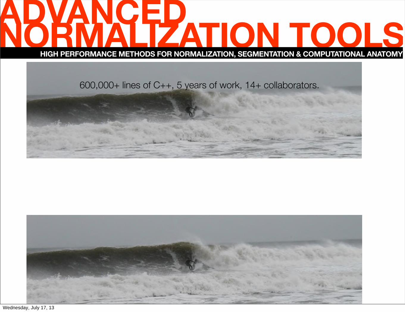
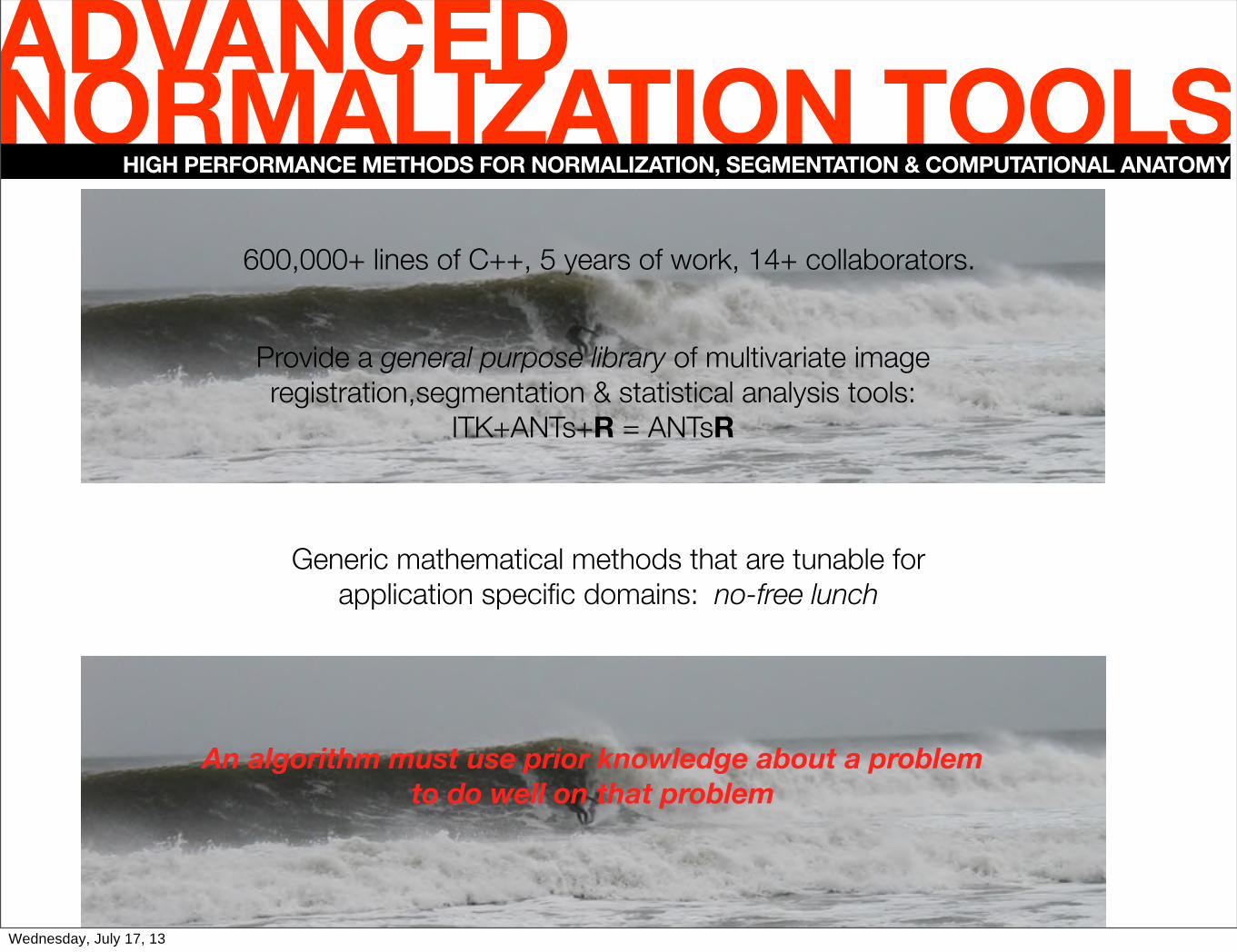
600,000+ lines of C++, 5 years of work, 14+ collaborators.
ADVANCEDNORMALIZATION TOOLSHIGH PERFORMANCE METHODS FOR NORMALIZATION, SEGMENTATION & COMPUTATIONAL ANATOMY
Wednesday, July 17, 13

600,000+ lines of C++, 5 years of work, 14+ collaborators.
Provide a general purpose library of multivariate image registration,segmentation & statistical analysis tools:
ITK+ANTs+R = ANTsR
Generic mathematical methods that are tunable for application specific domains: no-free lunch
ADVANCEDNORMALIZATION TOOLSHIGH PERFORMANCE METHODS FOR NORMALIZATION, SEGMENTATION & COMPUTATIONAL ANATOMY
Wednesday, July 17, 13
600,000+ lines of C++, 5 years of work, 14+ collaborators.
Provide a general purpose library of multivariate image registration,segmentation & statistical analysis tools:
ITK+ANTs+R = ANTsR
Generic mathematical methods that are tunable for application specific domains: no-free lunch
An algorithm must use prior knowledge about a problem to do well on that problem
ADVANCEDNORMALIZATION TOOLSHIGH PERFORMANCE METHODS FOR NORMALIZATION, SEGMENTATION & COMPUTATIONAL ANATOMY
Wednesday, July 17, 13

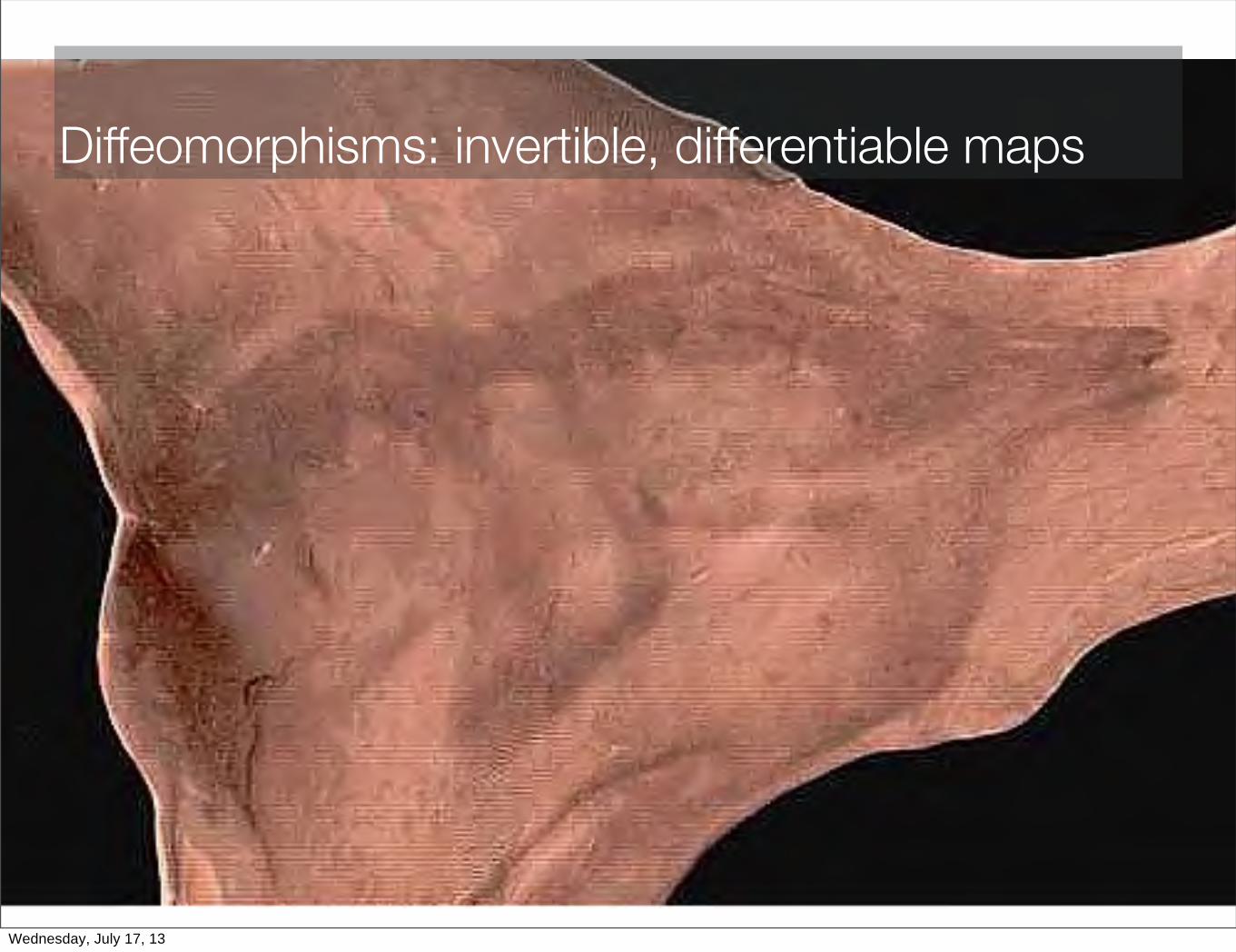
Diffeomorphisms: invertible, differentiable maps
Wednesday, July 17, 13
Diffeomorphisms: invertible, differentiable maps
Wednesday, July 17, 13

Diffeomorphisms: invertible, differentiable maps
Defines a metric
Wednesday, July 17, 13

Diffeomorphisms: invertible, differentiable maps
Defines a metric
Infinite-dimensional = flexible
Wednesday, July 17, 13

ANTs-SyN captures large brain differences
v4
Wednesday, July 17, 13
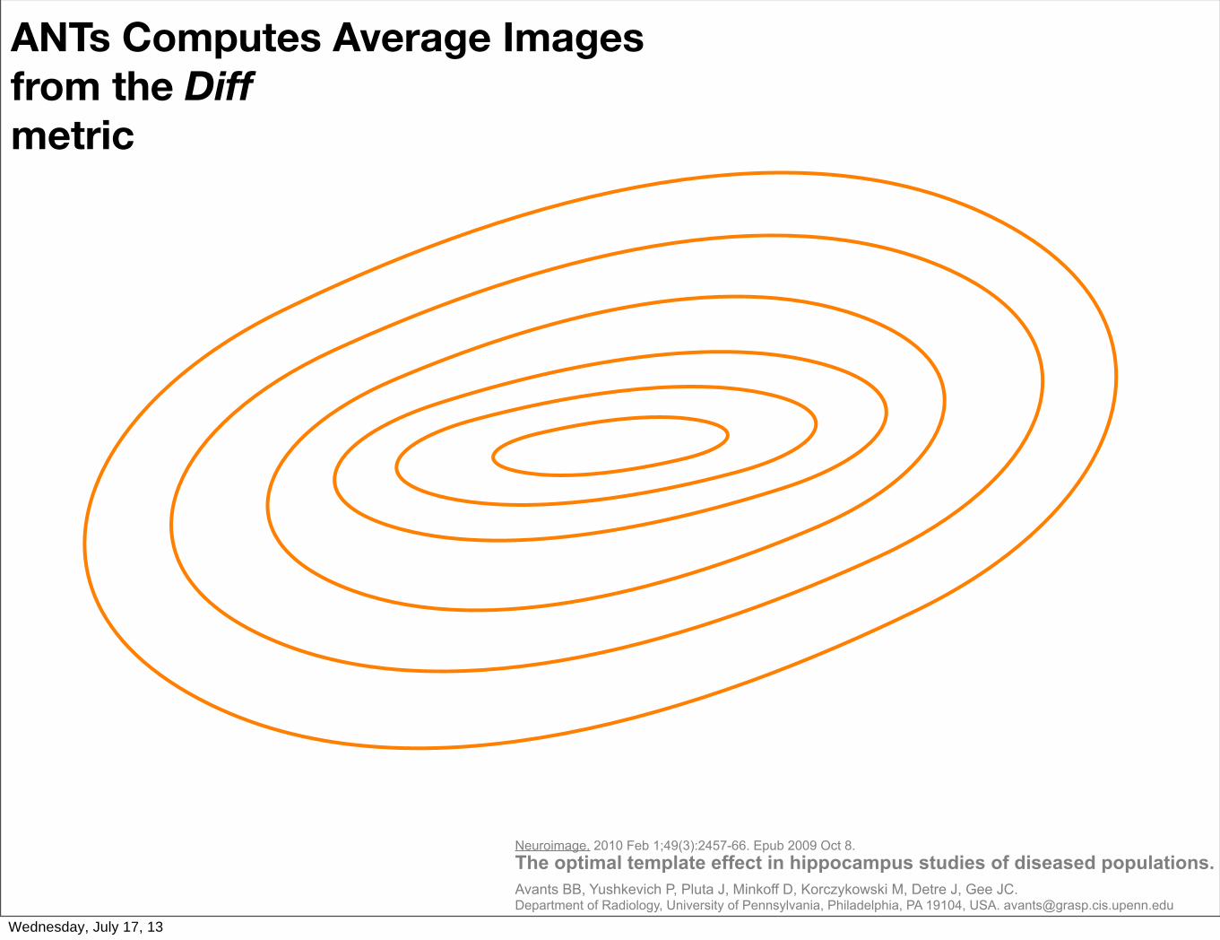
Neuroimage. 2010 Feb 1;49(3):2457-66. Epub 2009 Oct 8.The optimal template effect in hippocampus studies of diseased populations.Avants BB, Yushkevich P, Pluta J, Minkoff D, Korczykowski M, Detre J, Gee JC.Department of Radiology, University of Pennsylvania, Philadelphia, PA 19104, USA. [email protected]
ANTs Computes Average Imagesfrom the Diff metric
Wednesday, July 17, 13
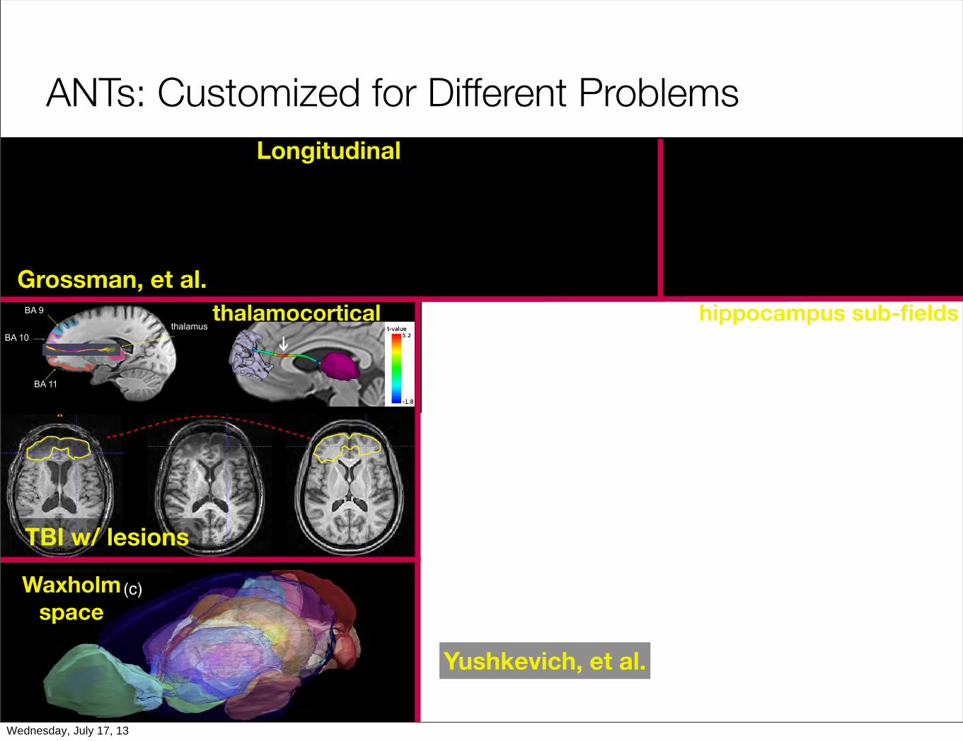
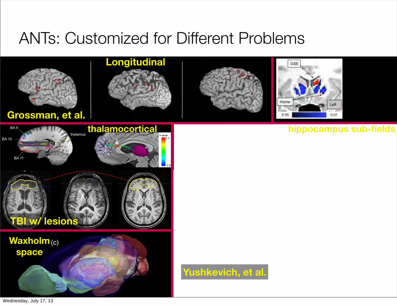
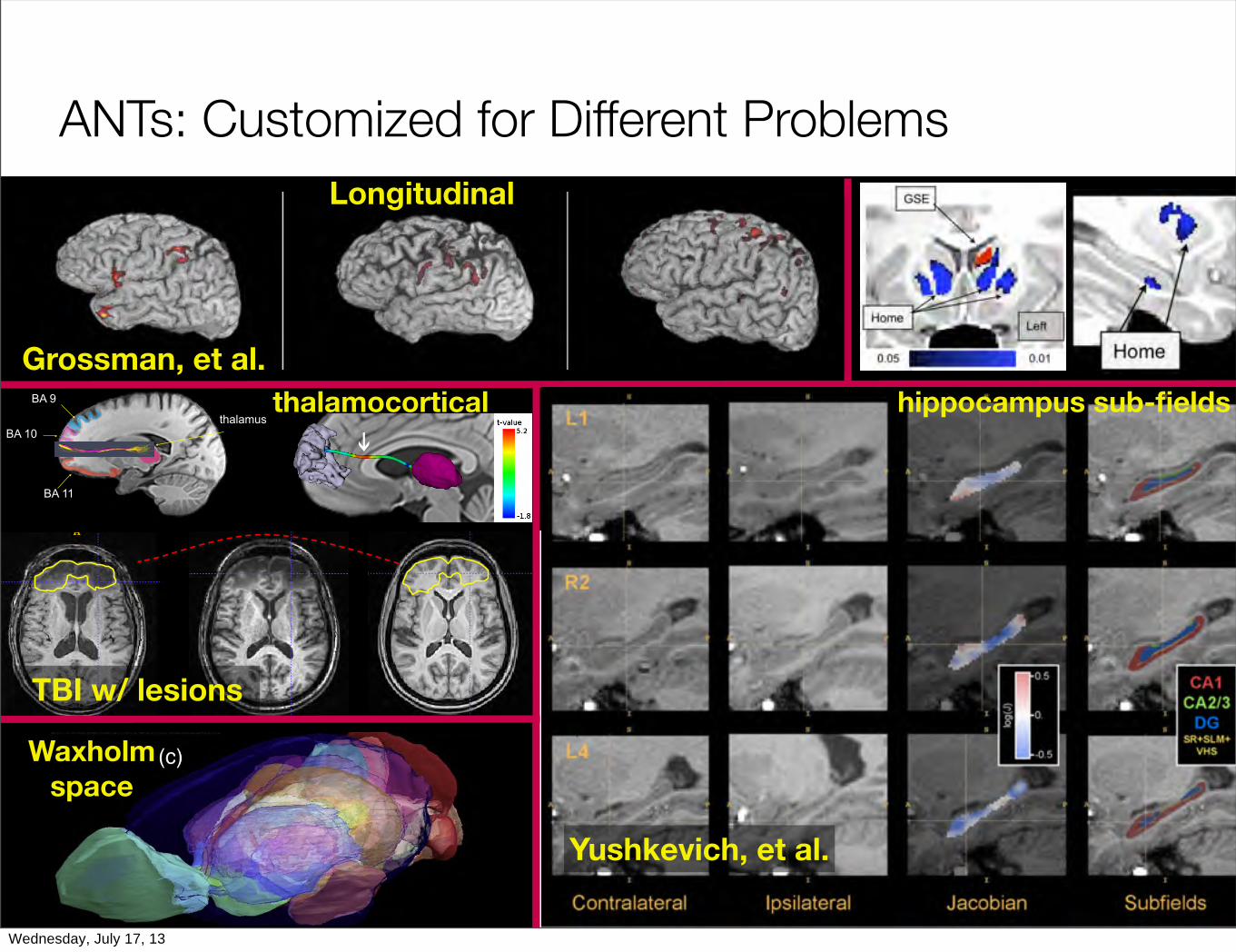
ANTs: Customized for Different Problems
Yushkevich, et al.
Grossman, et al.
TBI w/ lesions
Longitudinal
thalamocortical hippocampus sub-fields
Waxholmspace
Wednesday, July 17, 13

ANTs: Customized for Different Problems
Yushkevich, et al.
Grossman, et al.
TBI w/ lesions
Longitudinal
thalamocortical hippocampus sub-fields
Waxholmspace
Wednesday, July 17, 13
ANTs: Customized for Different Problems
BA 9
BA 10
BA 11
thalamus
Yushkevich, et al.
Grossman, et al.
TBI w/ lesions
Longitudinal
thalamocortical hippocampus sub-fields
Waxholmspace
Wednesday, July 17, 13

ANTs: Customized for Different Problems
BA 9
BA 10
BA 11
thalamus
Yushkevich, et al.
Grossman, et al.
TBI w/ lesions
Longitudinal
thalamocortical hippocampus sub-fields
Waxholmspace
Wednesday, July 17, 13
ANTs: Customized for Different Problems
BA 9
BA 10
BA 11
thalamus
Yushkevich, et al.
Grossman, et al.
TBI w/ lesions
Longitudinal
thalamocortical hippocampus sub-fields
Waxholmspace
Wednesday, July 17, 13

ANTs: Customized for Different Problems
BA 9
BA 10
BA 11
thalamus
Yushkevich, et al.
Grossman, et al.
TBI w/ lesions
Longitudinal
thalamocortical hippocampus sub-fields
Waxholmspace
Wednesday, July 17, 13
ANTs: Customized for Different Problems
BA 9
BA 10
BA 11
thalamus
Yushkevich, et al.
Grossman, et al.
TBI w/ lesions
Longitudinal
thalamocortical hippocampus sub-fields
Waxholmspace
Wednesday, July 17, 13

Part 1b: ANTs in Independent Evaluation
Wednesday, July 17, 13

“Would you like to participate in an unbiased evaluation of deformable registration?”
- Arno Klein, Nov 2008
Klein Evaluation 2009
Wednesday, July 17, 13

“Would you like to participate in an unbiased evaluation of deformable registration?”
- Arno Klein, Nov 2008
Klein Evaluation 2009
One of the most cited neuroimage papers since 2008
Wednesday, July 17, 13

Arno’s Algorithm Fight Club
Wednesday, July 17, 13

Open-Access Labeled Datasets
Wednesday, July 17, 13

Klein Evaluation Results
Wednesday, July 17, 13

Klein Evaluation Results
Wednesday, July 17, 13
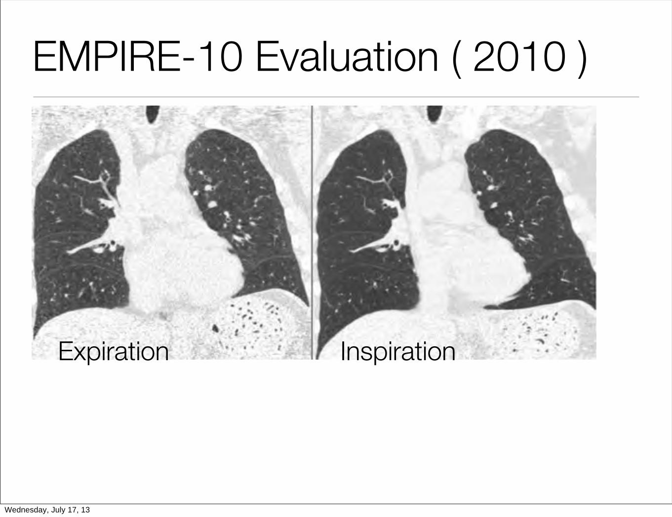
EMPIRE-10 Evaluation ( 2010 )
Expiration Inspiration
Wednesday, July 17, 13

EMPIRE-10 Evaluation ( 2010 )
• Register pairs of thoracic CT volumes
Expiration Inspiration
Wednesday, July 17, 13

EMPIRE-10 Evaluation ( 2010 )
• Register pairs of thoracic CT volumes• Part of MICCAI 2010 Grand Challenges: http://empire10.isi.uu.nl
Expiration Inspiration
Wednesday, July 17, 13

EMPIRE-10 Evaluation ( 2010 )
• Register pairs of thoracic CT volumes• Part of MICCAI 2010 Grand Challenges: http://empire10.isi.uu.nl
• First round offline competition finished on June 21, 2010
Expiration Inspiration
Wednesday, July 17, 13

EMPIRE-10 Evaluation ( 2010 )
• Register pairs of thoracic CT volumes• Part of MICCAI 2010 Grand Challenges: http://empire10.isi.uu.nl
• First round offline competition finished on June 21, 2010• ANTS by picsl gsyn : 1st place among 34 teams
Expiration Inspiration
Wednesday, July 17, 13

EMPIRE-10 Evaluation
boundaries fissures landmarks jacobian
Wednesday, July 17, 13

EMPIRE-10 Evaluation
boundaries fissures landmarks jacobian
Wednesday, July 17, 13

SATA 2012: Multi-Atlas ChallengeAtlas 1 Atlas k. . .
Registration and Warping
Registration and Warping
Candidate Segmentation
Candidate Segmentation
Joint Label Fusion
Consensus Segmentation
Target Image
Landman, Warfield
Wednesday, July 17, 13

SATA 2012: Multi-Atlas ChallengeAtlas 1 Atlas k. . .
Registration and Warping
Registration and Warping
Candidate Segmentation
Candidate Segmentation
Joint Label Fusion
Consensus Segmentation
Target Image
Landman, Warfield
segmentation
Wednesday, July 17, 13

SATA 2012: Multi-Atlas ChallengeAtlas 1 Atlas k. . .
Registration and Warping
Registration and Warping
Candidate Segmentation
Candidate Segmentation
Joint Label Fusion
Consensus Segmentation
Target Image
Landman, Warfield
segmentation
Wednesday, July 17, 13
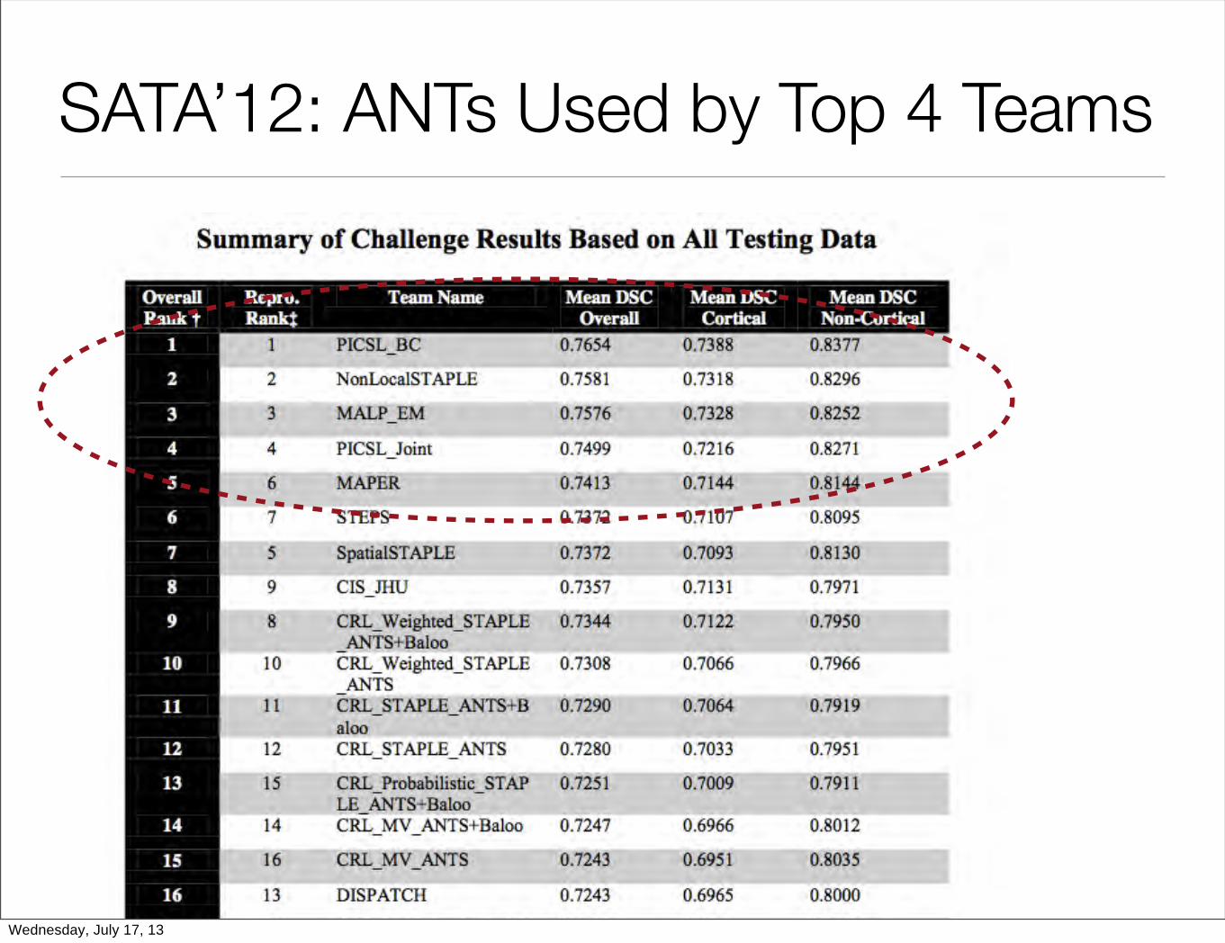
SATA’12: ANTs Used by Top 4 Teams
Wednesday, July 17, 13

SATA’12: ANTs Used by Top 4 Teams
Wednesday, July 17, 13

SATA Challenge MICCAI 2013:ANTs Provides Standardized Registration
1,600 registrations
1600 “easy” registrations
Wednesday, July 17, 13

SATA Challenge MICCAI 2013:ANTs Provides Standardized Registration
7,000+ multivariate registrations (challenging)
Expected Results for challenge participants ~ Dice = 0.8+
1,600 registrations
1600 “easy” registrations
Wednesday, July 17, 13

SATA Challenge MICCAI 2013:ANTs Provides Standardized Registration
7,000+ multivariate registrations (challenging)
Expected Results for challenge participants ~ Dice = 0.8+
1,600 registrations
1600 “easy” registrations
13,000+ 4D registrations (very challenging)
Wednesday, July 17, 13
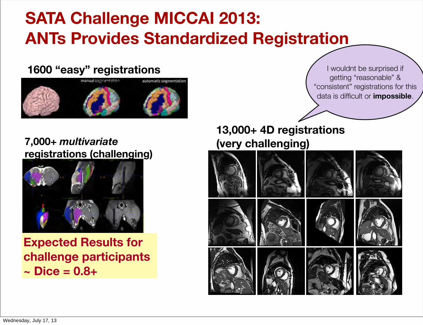
SATA Challenge MICCAI 2013:ANTs Provides Standardized Registration
7,000+ multivariate registrations (challenging)
Expected Results for challenge participants ~ Dice = 0.8+
I wouldnt be surprised if getting “reasonable” &
“consistent” registrations for this data is difficult or impossible.
1,600 registrations
1600 “easy” registrations
13,000+ 4D registrations (very challenging)
Heart orientation varies between individuals
Wednesday, July 17, 13
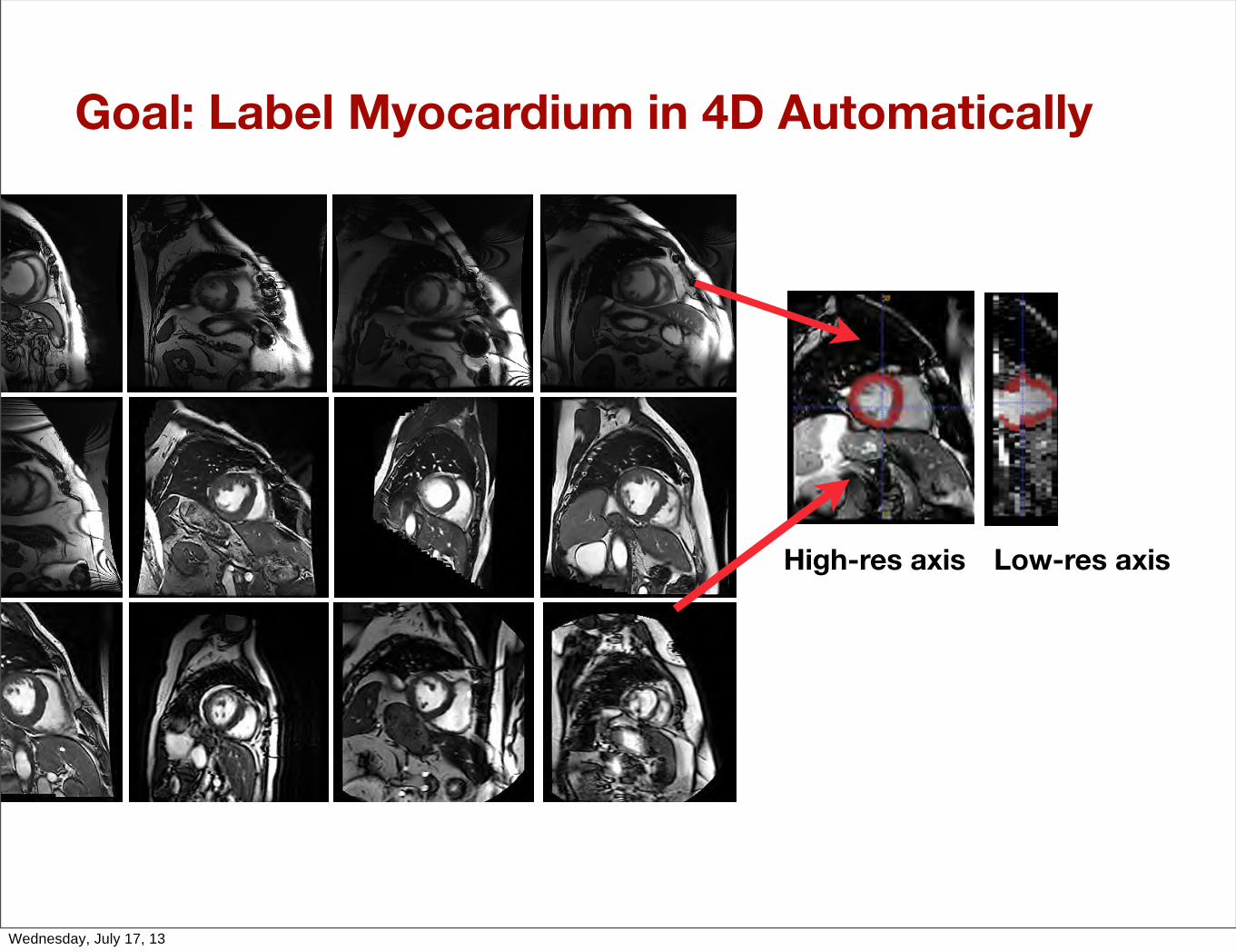
Goal: Label Myocardium in 4D Automatically
High-res axis Low-res axis
Wednesday, July 17, 13

Goal: Label Myocardium in 4D Automatically
High-res axis Low-res axis
Wednesday, July 17, 13
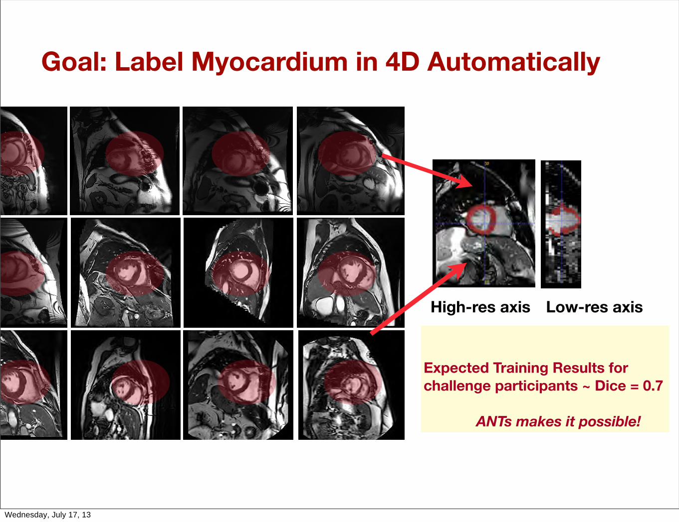
Goal: Label Myocardium in 4D Automatically
High-res axis Low-res axis
Expected Training Results for challenge participants ~ Dice = 0.7
ANTs makes it possible!
Wednesday, July 17, 13

Goal: Label Myocardium in 4D Automatically
High-res axis Low-res axis
Expected Training Results for challenge participants ~ Dice = 0.7
ANTs makes it possible!
Maximum efficiency with minimum wasted effort: ITKv4, Code ReuseWednesday, July 17, 13

Goal: Label Myocardium in 4D Automatically
High-res axis Low-res axis
Expected Training Results for challenge participants ~ Dice = 0.7
ANTs makes it possible!
Maximum efficiency with minimum wasted effort: ITKv4, Code Reuse
over 20,000 registrations performed in a short time period - most on problems we had not seen before
Wednesday, July 17, 13
Part 2: Ants - Integrated Method Set for Large-Scale MM-Image Quantification
Wednesday, July 17, 13

DiReCTcortical thickness
Dog Monkey Adolescent Human Middle-Aged HumanChimpRat Neurodegeneration4 Week Old Human
Mean Thickness: rat=1.7mm dog=2.0mm, monkey=3.0mm, chimp=3.5mm, adol=3.4mm, mid-age=3.0mm, ndgen=2.6mm
Dog Monkey Adolescent Human Middle-Aged HumanChimpRat Neurodegeneration4 Week Old Human
Mean Thickness: rat=1.7mm dog=2.0mm, monkey=3.0mm, chimp=3.5mm, adol=3.4mm, mid-age=3.0mm, ndgen=2.6mm
Relatively ThickerRelatively Thinner
Goal: Easily Customizable, Reliable Software for Any Modality, Species, Data Type etc.
Wednesday, July 17, 13

DiReCTcortical thickness
“easy” data
Dog Monkey Adolescent Human Middle-Aged HumanChimpRat Neurodegeneration4 Week Old Human
Mean Thickness: rat=1.7mm dog=2.0mm, monkey=3.0mm, chimp=3.5mm, adol=3.4mm, mid-age=3.0mm, ndgen=2.6mm
Dog Monkey Adolescent Human Middle-Aged HumanChimpRat Neurodegeneration4 Week Old Human
Mean Thickness: rat=1.7mm dog=2.0mm, monkey=3.0mm, chimp=3.5mm, adol=3.4mm, mid-age=3.0mm, ndgen=2.6mm
Relatively ThickerRelatively Thinner
Goal: Easily Customizable, Reliable Software for Any Modality, Species, Data Type etc.
Wednesday, July 17, 13

N4 = N3++
Atropos
ANTs Big Three: Registration, Segmentation, Bias Correction
Wednesday, July 17, 13

N4 = N3++
Atroposprior
knowledge
Maximum efficiency with minimum wasted effort. - Jigaro Kano
ANTs Big Three: Registration, Segmentation, Bias Correction
Wednesday, July 17, 13

N4 = N3++
Atroposprior
knowledge
Maximum efficiency with minimum wasted effort. - Jigaro Kano
ITKv4, Slicer, NiPy, NeuroDebian, InVicro, AmGen, Pfizer ....
ANTs Big Three: Registration, Segmentation, Bias Correction
Wednesday, July 17, 13

Initial N4bias correction
Registration-based skull stripping
N4 bias correction(segmentation step)
Input anatomical MRI
Output thickness mapyes
no
T1 template
Convergence or > n iterations?
Atropos 3-tissuesegmentation
DiReCT
Registration mask (optional)
Brain prior CSF prior GM prior WM prior
N4 tissue maskcalculation
antsAtroposN4.shantsBrainExtraction.sh
antsCorticalThickness.sh
antsMultivariateTemplateConstruction.sh
The ANTs Cortical Thickness Pipeline
Hopkins & Avants, J of NSci, 2013
postcentral gyri compared with all other cortical regions (Fig. 4). Inaddition, a significant two-way interaction was found between sexand region F(11,759) ! 2.28, p " 0.009 (Fig. 4). Subsequent post hocanalysis indicated no significant differences between males and fe-males for any of the regions.
Adjusted thickness measuresLuders et al. (2006b) found that regionaland sex differences in cortical thickness canbe influenced when adjustments are madefor variation in brain volume. To addressthis specific issue, we conducted a secondanalysis examining sex and regional varia-tion after adjusting for total gray and whitematter volume. For this analysis, we reranthe mixed-model ANOVA using the thick-ness values as the repeated measure whilesex was the between group factor, but weincluded brain volume as a covariate. As be-fore, we found a significant main effect forregion F(11,759) ! 242.18, p " 0.001 and asignificant two-way interaction between sexand region F(11,759) ! 3.57, p " 0.001. Maleswere found to have thicker cortex than fe-males for the precentral and postcentral gyrias well as the superior parietal lobe. In con-trast, females were found to have thickerdorsal PFC than males.
Lateralization in cortical thicknessWe next considered asymmetries in eachof the regions. After adjusting ! for mul-tiple comparisons, one sample t tests onthe AQ scores revealed significant right-ward asymmetries in cortical thickness for10 of the 12 regions including orbital and
dorsal prefrontal cortex, precentral and postcentral gyri, superiorparietal lobe, supramarginal gyrus, superior temporal gyrus,middle temporal gyrus, inferior frontal gyrus, and posterior su-perior temporal gyrus (Table 1). The rightward asymmetries in
Figure 4. Mean cortical thickness of the left and right hemispheres. Color bar indicates variation in cortical thickness throughout cortex. Top, Left and right lateral view. Bottom, Left and rightmedial views.
Figure 5. Mean cortical thickness (#SE) for male and female chimpanzees for each of the 12 regions. Bolded labels indicatesignificant male-female differences at p " 0.05 after adjustment for overall brain volume.
Hopkins and Avants • Cortical Thickness in Chimpanzees J. Neurosci., March 20, 2013 • 33(12):5241–5248 • 5245
Wednesday, July 17, 13

Initial N4bias correction
Registration-based skull stripping
N4 bias correction(segmentation step)
Input anatomical MRI
Output thickness mapyes
no
T1 template
Convergence or > n iterations?
Atropos 3-tissuesegmentation
DiReCT
Registration mask (optional)
Brain prior CSF prior GM prior WM prior
N4 tissue maskcalculation
antsAtroposN4.shantsBrainExtraction.sh
antsCorticalThickness.sh
antsMultivariateTemplateConstruction.sh
The ANTs Cortical Thickness Pipeline
Wednesday, July 17, 13

HOME @ Age 4 weeks ~ CSF, WM, GM Volume ?
Cohort: 17 low-SES African-American females who were imaged @ age 4 weeks. T2, DTI, BOLD, T1 neuroimaging, swaddling, etc.
Analyses
22 24 26 28 30
20
22
24
26
28
30
32
TOT 8 fold cross−validation predicted Home vs real Home
crossValHomere
alH
ome
● ●
●
●
●
●
●
●
●
●
●
●
●
●
●
Local atlas
Probability maps 24 T2 subjects (bias field corrected)
Wednesday, July 17, 13

1200+ images, Many Scanners => 2 failuresIXI Kirby NKI Oasis
Templates for each data source: Ages 8 - 80Wednesday, July 17, 13

ANTs: Map Anatomy to Other Modalitiesfrom JJ Wang’sPediatric Templateof Perfusion
Wednesday, July 17, 13

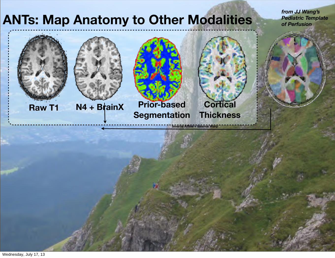
ANTs: Map Anatomy to Other Modalities
CorticalThickness
Raw T1 N4 + BrainX Prior-basedSegmentation
Inverse Affine + Inverse Warp
from JJ Wang’sPediatric Templateof Perfusion
Wednesday, July 17, 13
ANTs: Map Anatomy to Other Modalities
CorticalThickness
Raw T1 N4 + BrainX Prior-basedSegmentation
Inverse Affine + Inverse Warp
from JJ Wang’sPediatric Templateof Perfusion
Wednesday, July 17, 13
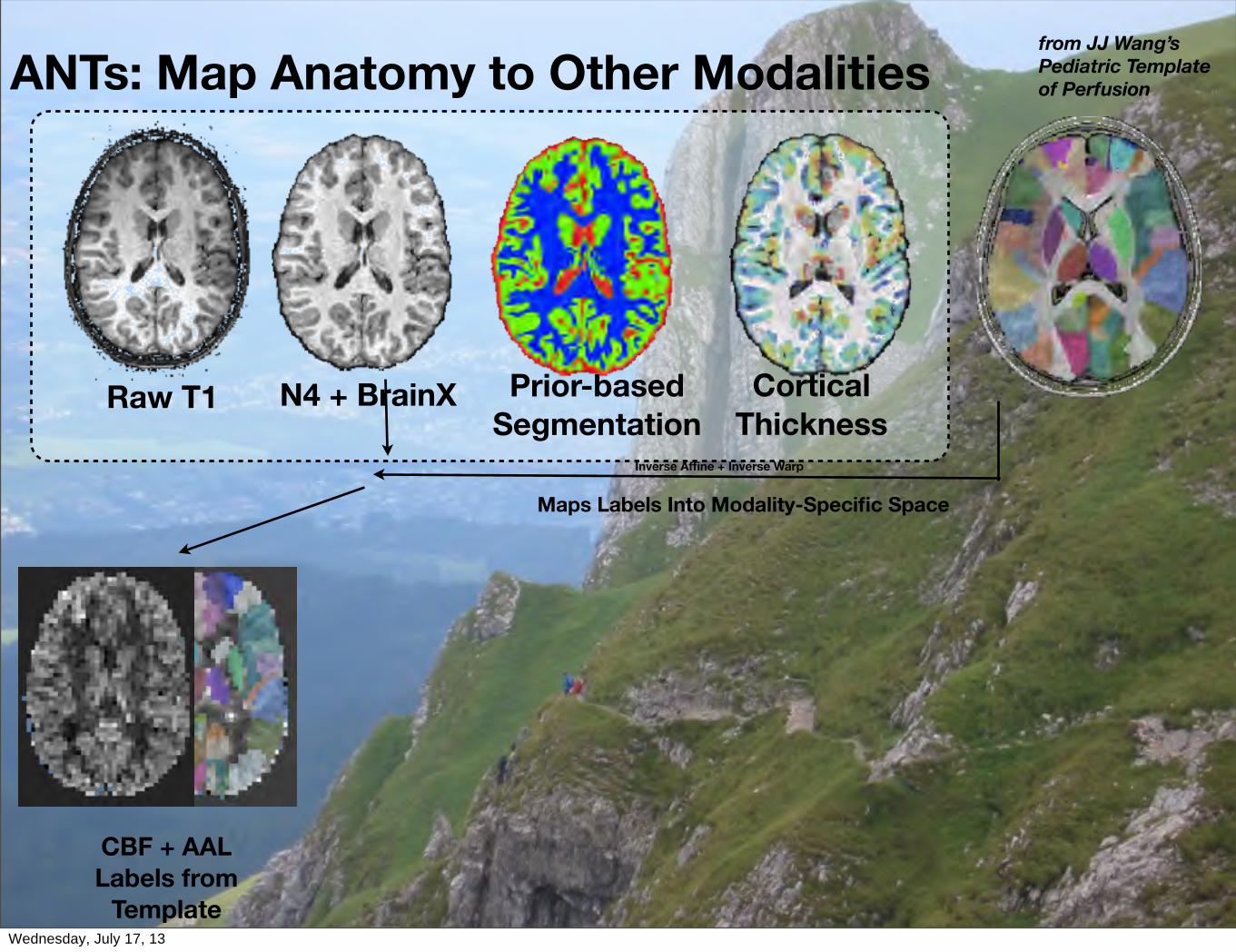
ANTs: Map Anatomy to Other Modalities
CorticalThickness
Raw T1 N4 + BrainX Prior-basedSegmentation
Inverse Affine + Inverse Warp
Maps Labels Into Modality-Specific Space
CBF + AALLabels from
Template
from JJ Wang’sPediatric Templateof Perfusion
Wednesday, July 17, 13

ANTs: Map Anatomy to Other Modalities
CorticalThickness
Raw T1 N4 + BrainX Prior-basedSegmentation
Inverse Affine + Inverse Warp
BOLD + AALLabels from
Template
Maps Labels Into Modality-Specific Space
CBF + AALLabels from
Template
from JJ Wang’sPediatric Templateof Perfusion
Wednesday, July 17, 13

ANTs: Map Anatomy to Other Modalities
CorticalThickness
Raw T1 N4 + BrainX Prior-basedSegmentation
Inverse Affine + Inverse Warp
FA from DTI + AALLabels from Template
BOLD + AALLabels from
Template
Maps Labels Into Modality-Specific Space
CBF + AALLabels from
Template
from JJ Wang’sPediatric Templateof Perfusion
Wednesday, July 17, 13

ANTs: Map Anatomy to Other Modalities
CorticalThickness
Raw T1 N4 + BrainX Prior-basedSegmentation
Inverse Affine + Inverse Warp
MTR + AALFA from DTI + AALLabels from Template
BOLD + AALLabels from
Template
Maps Labels Into Modality-Specific Space
CBF + AALLabels from
Template
from JJ Wang’sPediatric Templateof Perfusion
Wednesday, July 17, 13
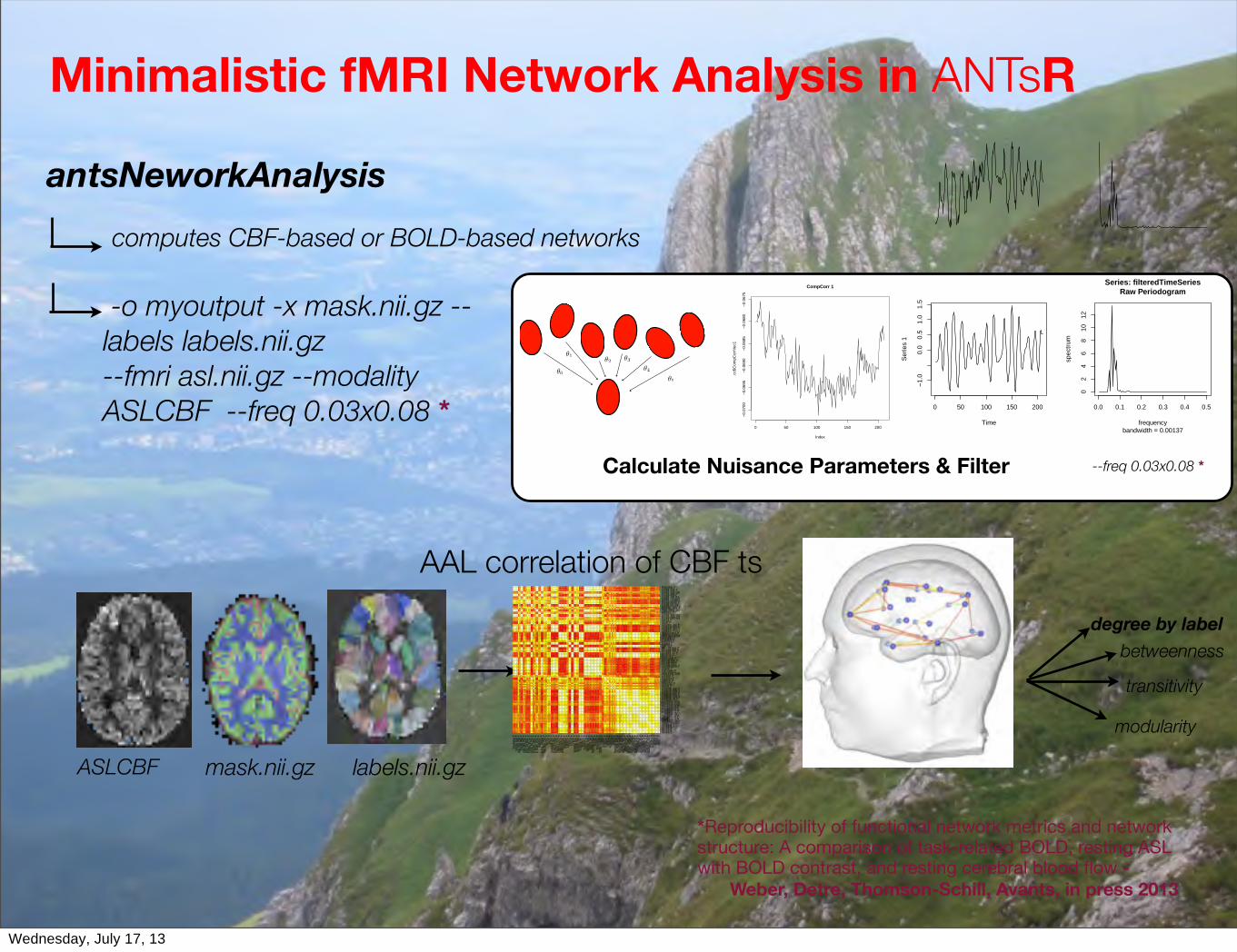
antsNeworkAnalysiscomputes CBF-based or BOLD-based networks
-o myoutput -x mask.nii.gz --labels labels.nii.gz --fmri asl.nii.gz --modality ASLCBF --freq 0.03x0.08 *
*Reproducibility of functional network metrics and network structure: A comparison of task-related BOLD, resting ASL with BOLD contrast, and resting cerebral blood flow -
Weber, Detre, Thomson-Schill, Avants, in press 2013
Calculate Nuisance Parameters & Filter
✓5
✓4
✓3✓2✓1
✓0
0 50 100 150 200
−0.0
700
−0.0
695
−0.0
690
−0.0
685
−0.0
680
−0.0
675
CompCorr 1
Index
cc$C
ompC
orrV
ec1
Time
myT
imeS
erie
s
0 50 100 150 200
−2−1
01
0.0 0.1 0.2 0.3 0.4 0.5
05
1015
frequency
spec
trum
Series: myTimeSeriesRaw Periodogram
bandwidth = 0.00137
Time
Serie
s 1
0 50 100 150 200
−1.0
0.0
0.5
1.0
1.5
0.0 0.1 0.2 0.3 0.4 0.5
02
46
810
12
frequency
spec
trum
Series: filteredTimeSeriesRaw Periodogram
bandwidth = 0.00137
Prec
entra
l_R
Prec
entra
l_L
Fron
tal_
Sup_
RFr
onta
l_Su
p_L
Fron
tal_
Sup_
Orb
_RFr
onta
l_Su
p_O
rb_L
Fron
tal_
Mid
_RFr
onta
l_M
id_L
Fron
tal_
Mid
_Orb
_RFr
onta
l_M
id_O
rb_L
Fron
tal_
Inf_
Ope
r_R
Fron
tal_
Inf_
Ope
r_L
Fron
tal_
Inf_
Tri_
RFr
onta
l_In
f_Tr
i_L
Fron
tal_
Inf_
Orb
_RFr
onta
l_In
f_O
rb_L
Rol
andi
c_O
per_
RR
olan
dic_
Ope
r_L
Supp
_Mot
or_A
rea_
RSu
pp_M
otor
_Are
a_L
Olfa
ctor
y_R
Olfa
ctor
y_L
Fron
tal_
Sup_
Med
ial_
RFr
onta
l_Su
p_M
edia
l_L
Fron
tal_
Med
_Orb
_RFr
onta
l_M
ed_O
rb_L
Rec
tus_
RR
ectu
s_L
Insu
la_R
Insu
la_L
Cin
gulu
m_A
nt_R
Cin
gulu
m_A
nt_L
Cin
gulu
m_M
id_R
Cin
gulu
m_M
id_L
Cin
gulu
m_P
ost_
RC
ingu
lum
_Pos
t_L
Hip
poca
mpu
s_R
Hip
poca
mpu
s_L
Para
Hip
poca
mpa
l_R
Para
Hip
poca
mpa
l_L
Amyg
dala
_RAm
ygda
la_L
Cal
carin
e_R
Cal
carin
e_L
Cun
eus_
RC
uneu
s_L
Ling
ual_
RLi
ngua
l_L
Occ
ipita
l_Su
p_R
Occ
ipita
l_Su
p_L
Occ
ipita
l_M
id_R
Occ
ipita
l_M
id_L
Occ
ipita
l_In
f_R
Occ
ipita
l_In
f_L
Fusi
form
_RFu
sifo
rm_L
Post
cent
ral_
RPo
stce
ntra
l_L
Parie
tal_
Sup_
RPa
rieta
l_Su
p_L
Parie
tal_
Inf_
RPa
rieta
l_In
f_L
Supr
aMar
gina
l_R
Supr
aMar
gina
l_L
Angu
lar_
RAn
gula
r_L
Prec
uneu
s_R
Prec
uneu
s_L
Para
cent
ral_
Rob
ule_
RPa
race
ntra
l_R
obul
e_L
Cau
date
_RC
auda
te_L
Puta
men
_RPu
tam
en_L
Pallid
um_R
Pallid
um_L
Thal
amus
_RTh
alam
us_L
Hes
chl_
RH
esch
l_L
Tem
pora
l_Su
p_R
Tem
pora
l_Su
p_L
Tem
pora
l_Po
le_S
up_R
Tem
pora
l_Po
le_S
up_L
Tem
pora
l_M
id_R
Tem
pora
l_M
id_L
Tem
pora
l_Po
le_M
id_R
Tem
pora
l_Po
le_M
id_L
Tem
pora
l_In
f_R
Tem
pora
l_In
f_L
Cer
ebel
um_C
rus1
_RC
ereb
elum
_Cru
s1_L
Cer
ebel
um_C
rus2
_RC
ereb
elum
_Cru
s2_L
Cer
ebel
um_3
_RC
ereb
elum
_3_L
Cer
ebel
um_4
_5_R
Cer
ebel
um_4
_5_L
Cer
ebel
um_6
_RC
ereb
elum
_6_L
Cer
ebel
um_7
b_R
Cer
ebel
um_7
b_L
Cer
ebel
um_8
_RC
ereb
elum
_8_L
Cer
ebel
um_9
_RC
ereb
elum
_9_L
Cer
ebel
um_1
0_R
Cer
ebel
um_1
0_L
Verm
is_1
_2Ve
rmis
_3Ve
rmis
_4_5
Verm
is_6
Verm
is_7
Verm
is_8
Verm
is_9
Verm
is_1
0
Vermis_10Vermis_9Vermis_8Vermis_7Vermis_6Vermis_4_5Vermis_3Vermis_1_2Cerebelum_10_LCerebelum_10_RCerebelum_9_LCerebelum_9_RCerebelum_8_LCerebelum_8_RCerebelum_7b_LCerebelum_7b_RCerebelum_6_LCerebelum_6_RCerebelum_4_5_LCerebelum_4_5_RCerebelum_3_LCerebelum_3_RCerebelum_Crus2_LCerebelum_Crus2_RCerebelum_Crus1_LCerebelum_Crus1_RTemporal_Inf_LTemporal_Inf_RTemporal_Pole_Mid_LTemporal_Pole_Mid_RTemporal_Mid_LTemporal_Mid_RTemporal_Pole_Sup_LTemporal_Pole_Sup_RTemporal_Sup_LTemporal_Sup_RHeschl_LHeschl_RThalamus_LThalamus_RPallidum_LPallidum_RPutamen_LPutamen_RCaudate_LCaudate_RParacentral_Robule_LParacentral_Robule_RPrecuneus_LPrecuneus_RAngular_LAngular_RSupraMarginal_LSupraMarginal_RParietal_Inf_LParietal_Inf_RParietal_Sup_LParietal_Sup_RPostcentral_LPostcentral_RFusiform_LFusiform_ROccipital_Inf_LOccipital_Inf_ROccipital_Mid_LOccipital_Mid_ROccipital_Sup_LOccipital_Sup_RLingual_LLingual_RCuneus_LCuneus_RCalcarine_LCalcarine_RAmygdala_LAmygdala_RParaHippocampal_LParaHippocampal_RHippocampus_LHippocampus_RCingulum_Post_LCingulum_Post_RCingulum_Mid_LCingulum_Mid_RCingulum_Ant_LCingulum_Ant_RInsula_LInsula_RRectus_LRectus_RFrontal_Med_Orb_LFrontal_Med_Orb_RFrontal_Sup_Medial_LFrontal_Sup_Medial_ROlfactory_LOlfactory_RSupp_Motor_Area_LSupp_Motor_Area_RRolandic_Oper_LRolandic_Oper_RFrontal_Inf_Orb_LFrontal_Inf_Orb_RFrontal_Inf_Tri_LFrontal_Inf_Tri_RFrontal_Inf_Oper_LFrontal_Inf_Oper_RFrontal_Mid_Orb_LFrontal_Mid_Orb_RFrontal_Mid_LFrontal_Mid_RFrontal_Sup_Orb_LFrontal_Sup_Orb_RFrontal_Sup_LFrontal_Sup_RPrecentral_LPrecentral_R
transitivity
modularity
betweennessdegree by label
mask.nii.gz labels.nii.gz ASLCBF
--freq 0.03x0.08 *
Minimalistic fMRI Network Analysis in ANTsR
AAL correlation of CBF ts
Wednesday, July 17, 13

ASL-CBF Network Connectivity Relates to Subjective SES
MacArthur Ladder ~ age + gender + brain-volume + IQ + globalCBF + ThicknessAtRegion + degreeOfNetworkAtRegion
Wednesday, July 17, 13

ASL-CBF Network Connectivity Relates to Subjective SES
MacArthur Ladder ~ age + gender + brain-volume + IQ + globalCBF + ThicknessAtRegion + degreeOfNetworkAtRegion
n=49, 20 male, 29 female, age 11.4 +/- 2.5each subject imaged with 3T T1 MRI, PCASL
Wednesday, July 17, 13

ASL-CBF Network Connectivity Relates to Subjective SES
MacArthur Ladder ~ age + gender + brain-volume + IQ + globalCBF + ThicknessAtRegion + degreeOfNetworkAtRegion
n=49, 20 male, 29 female, age 11.4 +/- 2.5each subject imaged with 3T T1 MRI, PCASL
Anticipated Salience Networkto relate to Ladder
Wednesday, July 17, 13

ASL-CBF Network Connectivity Relates to Subjective SES
MacArthur Ladder ~ age + gender + brain-volume + IQ + globalCBF + ThicknessAtRegion + degreeOfNetworkAtRegion
n=49, 20 male, 29 female, age 11.4 +/- 2.5each subject imaged with 3T T1 MRI, PCASL
Network connectivity q-value: Ladder ~ Degree
Left Insula: 0.009 - Salience (+)Left Anterior Cingulum: 0.002 - Salience (-)Left Precuneus 0.002 - DMN
Anticipated Salience Networkto relate to Ladder
Wednesday, July 17, 13

Part 3: Eigenanatomy
Wednesday, July 17, 13

Structural & Functional Eigenanatomy
Wednesday, July 17, 13

Structural & Functional Eigenanatomy
PCA, CCA or regression with anatomical constraints.
Wednesday, July 17, 13

Structural & Functional Eigenanatomy
“Voxels that change together should hang together”
PCA, CCA or regression with anatomical constraints.
Wednesday, July 17, 13

Structural & Functional Eigenanatomy
“Voxels that change together should hang together”
“Clustering before hypothesis-testing, not hypothesis-testing then clustering”
PCA, CCA or regression with anatomical constraints.
Wednesday, July 17, 13

Structural & Functional Eigenanatomy
“Voxels that change together should hang together”
We have been studying this set of methods so that we may standardize its use in clinical studies/trials, etc.
“Clustering before hypothesis-testing, not hypothesis-testing then clustering”
PCA, CCA or regression with anatomical constraints.
Incarnations for functional data, structural data and longitudinal data.
Wednesday, July 17, 13

The Eigenanatomy Objective Function
Related to Ng+ ’09, Varoquax IPMI ’11, various Stanford work.
Regularizes non-negative sparse PCA objective with anatomical priors.
The simplest such ‘additive’ objective:
We contribute a novel and efficient “deflation” based algorithm for optimization of the objective. (implemented in ANTs!)
Subject’s time series matrix or a population matrix
Tunable Parameter, controls strength of prior.
ith Prior ROI vector.ith eigenvector or p-Eigen optimized prior ROI. Sparsity Parameter
v⇤i = argmax
vi,kvik=1vi
> �X>X+ ⇥ ·mim
>i
�vi � �⇥vi⇥1
Neuroimage 2013, submitted
PCA
Wednesday, July 17, 13

The Eigenanatomy Objective Function
Related to Ng+ ’09, Varoquax IPMI ’11, various Stanford work.
Regularizes non-negative sparse PCA objective with anatomical priors.
The simplest such ‘additive’ objective:
We contribute a novel and efficient “deflation” based algorithm for optimization of the objective. (implemented in ANTs!)
Subject’s time series matrix or a population matrix
Tunable Parameter, controls strength of prior.
ith Prior ROI vector.ith eigenvector or p-Eigen optimized prior ROI. Sparsity Parameter
v⇤i = argmax
vi,kvik=1vi
> �X>X+ ⇥ ·mim
>i
�vi � �⇥vi⇥1
Neuroimage 2013, submitted
PCA Anatomical Prior
Wednesday, July 17, 13

a method that addresses a major complaint about ICA
Wednesday, July 17, 13

Eigenanatomy for functional MRI:Diagnose MCI from DMN connectivity
Neuroimage 2013, submitted
Instead of ....
Wednesday, July 17, 13

Eigenanatomy for functional MRI:Diagnose MCI from DMN connectivity
Neuroimage 2013, submitted
Instead of ....
Wednesday, July 17, 13

Eigenanatomy for functional MRI:Diagnose MCI from DMN connectivity
Neuroimage 2013, submitted
Instead of .... p-Eigen modified ROIs (λ=0.5)
Wednesday, July 17, 13
Eigenanatomy for functional MRI:Diagnose MCI from DMN connectivity
Neuroimage 2013, submitted
Instead of .... p-Eigen modified ROIs (λ=0.5)
Network Measures Derived from p-Eigen perform:
Significantly better than hippocampal volume based features.
Significantly better than using either true AAL ROIs or using standard SPCA ROIs based network measures as features.
Wednesday, July 17, 13

Eigenanatomy DTI & Cortical ParcellationNeuroimage 2013, submitted
Instead of ....
Wednesday, July 17, 13

Eigenanatomy DTI & Cortical ParcellationNeuroimage 2013, submitted
Instead of ....
Wednesday, July 17, 13

Eigenanatomy DTI & Cortical ParcellationNeuroimage 2013, submitted
Instead of ....
Wednesday, July 17, 13

Eigenanatomy DTI, Cortex & PowerBrain 2013, submitted
Wednesday, July 17, 13

Eigenanatomy DTI, Cortex & PowerBrain 2013, submitted
We contrast diagnostic power of:
Wednesday, July 17, 13

Eigenanatomy DTI, Cortex & PowerBrain 2013, submitted
We contrast diagnostic power of:
global measures such as ventricular volume
Wednesday, July 17, 13

Eigenanatomy DTI, Cortex & PowerBrain 2013, submitted
We contrast diagnostic power of:
global measures such as ventricular volume
anatomical volumes of interest (VOIs) (e.g., hippocampus)
Wednesday, July 17, 13

Eigenanatomy DTI, Cortex & PowerBrain 2013, submitted
We contrast diagnostic power of:
global measures such as ventricular volume
anatomical volumes of interest (VOIs) (e.g., hippocampus)
Eigenanatomy “VOIs.”
Wednesday, July 17, 13

Eigenanatomy DTI, Cortex & PowerBrain 2013, submitted
We contrast diagnostic power of:
global measures such as ventricular volume
anatomical volumes of interest (VOIs) (e.g., hippocampus)
Eigenanatomy “VOIs.”
Generalizabilty of single modality or multiple modality model.
Wednesday, July 17, 13

Eigenanatomy DTI, Cortex & PowerBrain 2013, submitted
We contrast diagnostic power of:
global measures such as ventricular volume
anatomical volumes of interest (VOIs) (e.g., hippocampus)
Eigenanatomy “VOIs.”
Generalizabilty of single modality or multiple modality model.
After training, identify which approach has best power in test data.
Wednesday, July 17, 13

Eigenanatomy DTI, Cortex & PowerBrain 2013, submitted
Power of Neuroimaging Biomarkers McMillan et al. ! 30!
Table 3. Summary of test prediction results: Power (minimum sample size) and
classification accuracy for MRI, DTI, Global, and multimodal combination of measures.
Modality Method Minimum N AUC P Sensitivity Specificity Youden-J
Volumetric MRI
Data-Driven 28 0.745 0.007 69 86 55
Anatomical 83 0.692 0.034 92 50 42
DTI
Data-Driven 20 0.804 0.001 51 100 51
Anatomical 227 0.581 0.375 36 86 22
Global
GM Volume 201 0.626 0.164 46 86 32
Ventricular Volume 377 0.625 0.082 56 79 35
Multimodal
Data-Driven 22 0.864 0.000 92 79 71
Anatomical 79 0.663 0.073 62 79 41
Multi-modality Eigenanatomy regions for DTI & Thickness include: left parietal cortex, bilateral precuneus, left/right SLF, & body & genu of the corpus callosum. min-sample-size = 22 in test set vs 79 for traditional VOIs.
In training set - differences between approaches was greatly reduced.
Results: Multi-modality Eigenanatomy performs best!
Wednesday, July 17, 13
●
●
●
●
●
●
●●
●
●
●
●
●
●
●
●
●
●
●
●
●
●
●
●
●
●
●
● ●●
●
●
●
●
●●
●
●
●
●
●
●
●
●
●●
●
●
●
●
●
●
●
−2.0 −1.5 −1.0 −0.5 0.0 0.5 1.0
−30
−20
−10
010
2030
Residualized thickness vs cognitive stimulation
Home4CogStim
Res
idua
lized
Thi
ckne
ss ●●
●
●
●
●●
●
●
●
●
●
●
●
●
●●
●
●
●
● ●
●
●●
●
●
● ●
●
●
●●
●
●
●●
●
●
●
●●
●
●
●
●
●
●
●
●
●
●
●
−2.0 −1.5 −1.0 −0.5 0.0 0.5 1.0
−40
−20
020
40
Residualized thickness vs cognitive stimulation
Home4CogStim
Res
idua
lized
Thi
ckne
ss
●
●
●
●
●
●
●
●
●
●●
●
●
●
●
●
●
●
●
●
●
●
●
●●
●
●
●
●
●
●
●
●
●
●
●●
●
●
●
●
●
●
●
●●
●
●
●
●
●
●
●
−2.0 −1.5 −1.0 −0.5 0.0 0.5 1.0
−40
−20
020
40
Residualized thickness vs cognitive stimulation
Home4CogStim
Res
idua
lized
Thi
ckne
ss
R Orbitofronal vs CogStim R Mid-temporal vs CogStim L Ant Mid-temporal vs CogStim
L in
ferio
r tem
pora
l
Bila
tera
l fus
iform
gyr
us
Residualized cortical thickness against age 4 environmental stimulation for 3 most significant regions
Left
infe
rior t
empo
ral
Age 4 cognitive stimulation Age 4 cognitive stimulationAge 4 cognitive stimulation
Early Environmenal Stimulation & Cortical Thickness
LR
Lateral inferior temporal gyrus †Lateral inferior temporal gyrus
Lateral inferior temporal gyrus
Bilateral fusiform gyrus
Wednesday, July 17, 13

●
●
●
●
●
●
●●
●
●
●
●
●
●
●
●
●
●
●
●
●
●
●
●
●
●
●
● ●●
●
●
●
●
●●
●
●
●
●
●
●
●
●
●●
●
●
●
●
●
●
●
−2.0 −1.5 −1.0 −0.5 0.0 0.5 1.0
−30
−20
−10
010
2030
Residualized thickness vs cognitive stimulation
Home4CogStim
Res
idua
lized
Thi
ckne
ss ●●
●
●
●
●●
●
●
●
●
●
●
●
●
●●
●
●
●
● ●
●
●●
●
●
● ●
●
●
●●
●
●
●●
●
●
●
●●
●
●
●
●
●
●
●
●
●
●
●
−2.0 −1.5 −1.0 −0.5 0.0 0.5 1.0
−40
−20
020
40
Residualized thickness vs cognitive stimulation
Home4CogStim
Res
idua
lized
Thi
ckne
ss
●
●
●
●
●
●
●
●
●
●●
●
●
●
●
●
●
●
●
●
●
●
●
●●
●
●
●
●
●
●
●
●
●
●
●●
●
●
●
●
●
●
●
●●
●
●
●
●
●
●
●
−2.0 −1.5 −1.0 −0.5 0.0 0.5 1.0
−40
−20
020
40
Residualized thickness vs cognitive stimulation
Home4CogStim
Res
idua
lized
Thi
ckne
ss
R Orbitofronal vs CogStim R Mid-temporal vs CogStim L Ant Mid-temporal vs CogStim
L in
ferio
r tem
pora
l
Bila
tera
l fus
iform
gyr
us
Residualized cortical thickness against age 4 environmental stimulation for 3 most significant regions
Left
infe
rior t
empo
ral
Age 4 cognitive stimulation Age 4 cognitive stimulationAge 4 cognitive stimulation
Early Environmenal Stimulation & Cortical Thickness
LR
Lateral inferior temporal gyrus †Lateral inferior temporal gyrus
Lateral inferior temporal gyrus
Bilateral fusiform gyrusRelated to
Verbal Comprehension
Wednesday, July 17, 13

Conclusions
Wednesday, July 17, 13

Conclusions
“Talk is cheap, show me the code.” stnava.github.io.com/ANTs
Wednesday, July 17, 13

Conclusions
“Talk is cheap, show me the code.” stnava.github.io.com/ANTs
ANTs may be used for robust, large-scale analysis of multiple image types. Free & Open-Source.
Wednesday, July 17, 13

Conclusions
“Talk is cheap, show me the code.” stnava.github.io.com/ANTs
ANTs may be used for robust, large-scale analysis of multiple image types. Free & Open-Source.
Eigenanatomy is a powerful prior-based dimensionality reduction tool.
Wednesday, July 17, 13

Conclusions
“Talk is cheap, show me the code.” stnava.github.io.com/ANTs
ANTs: solid software foundation for translational applications & i-biomarkers
v4
ANTs
ANTs may be used for robust, large-scale analysis of multiple image types. Free & Open-Source.
Eigenanatomy is a powerful prior-based dimensionality reduction tool.
Wednesday, July 17, 13
Acknowledgments
James Gee
ParamveerDhillon
Nick Tustison
Gang Song
Phil Cook
Corey McMillan
Jeff Duda
Ben Kandel
Murray Grossman
grant acknowledgments: 5R01DA022807, 1R01MH080892, 5R01EB006266-04the Dana Foundation
Wednesday, July 17, 13

We can compare apples and oranges ...
Wednesday, July 17, 13

We can compare apples and oranges ...
Wednesday, July 17, 13
We can compare apples and oranges ...
Wednesday, July 17, 13

ITKv4 Registration: Encapsulated & Generalized
Wednesday, July 17, 13

ITKv4 Registration: Encapsulated & Generalized
Metrics
Wednesday, July 17, 13
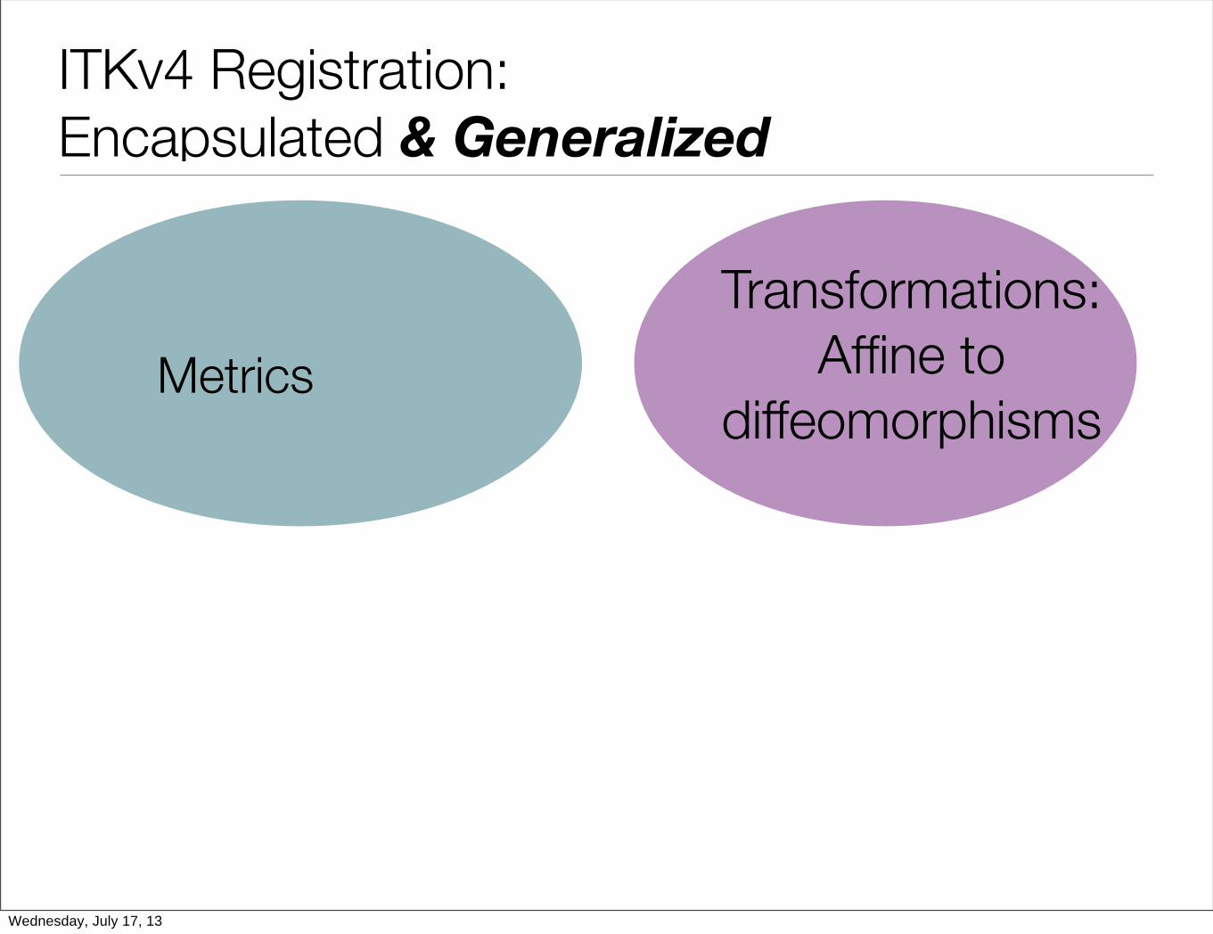
ITKv4 Registration: Encapsulated & Generalized
Metrics Transformations:
Affine to diffeomorphisms
Wednesday, July 17, 13
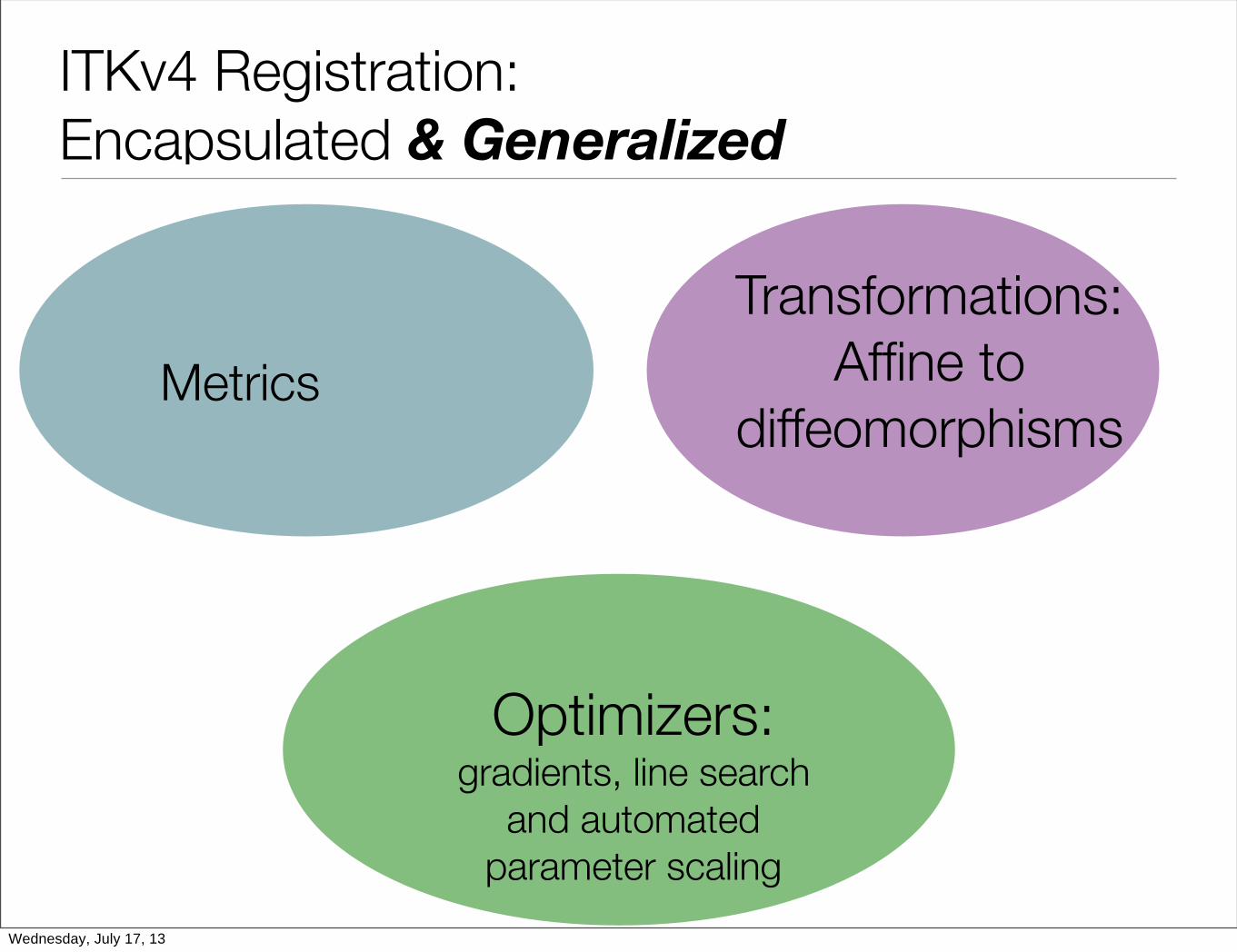
ITKv4 Registration: Encapsulated & Generalized
Metrics Transformations:
Affine to diffeomorphisms
Optimizers:gradients, line search
and automated parameter scaling
Wednesday, July 17, 13

ITKv4 Registration: Encapsulated & Generalized
Metrics Transformations:
Affine to diffeomorphisms
Optimizers:gradients, line search
and automated parameter scaling
●
●
●●
●
●
●●
●
●
●
●
●
●
●
●
●
●●
●
●
●
●
●
●
●
● ●
●●
●
●
●
●
●
●
●
●
●
●●
●
●
●
●
●
●
●
● ●
●
●
●
●
●
●●
●
●
●
●
●
●
●
●
●●
●
●
●
●
●
●
●
●
●
●
●
●
●
●
●
●
● ● ●
●
●
●
●
●
●
5 10 15 20
05
1015
2025
30
Predicting AnimalTotal from Brain
Predicted
Rea
l
Wednesday, July 17, 13
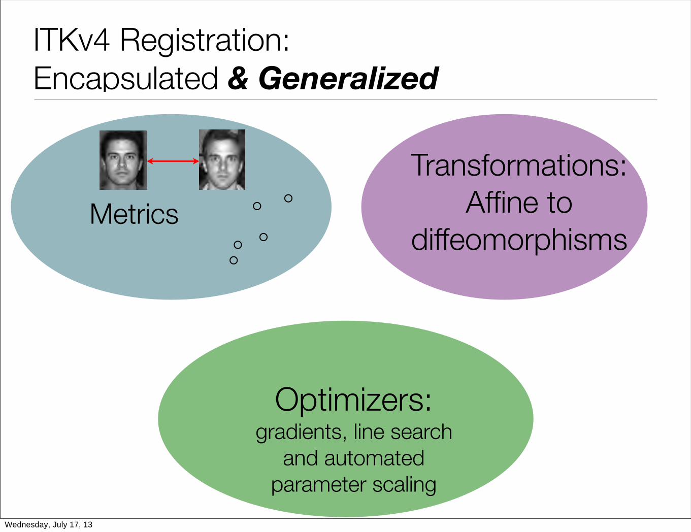
ITKv4 Registration: Encapsulated & Generalized
Metrics Transformations:
Affine to diffeomorphisms
Optimizers:gradients, line search
and automated parameter scaling
●
●
●●
●
●
●●
●
●
●
●
●
●
●
●
●
●●
●
●
●
●
●
●
●
● ●
●●
●
●
●
●
●
●
●
●
●
●●
●
●
●
●
●
●
●
● ●
●
●
●
●
●
●●
●
●
●
●
●
●
●
●
●●
●
●
●
●
●
●
●
●
●
●
●
●
●
●
●
●
● ● ●
●
●
●
●
●
●
5 10 15 20
05
1015
2025
30
Predicting AnimalTotal from Brain
Predicted
Rea
l
RGB
Wednesday, July 17, 13

ITKv4 Registration: Encapsulated & Generalized
Metrics Transformations:
Affine to diffeomorphisms
Optimizers:gradients, line search
and automated parameter scaling
Key Advance: all metrics are multi-threaded, may be computed from sparse or dense samples and used with low or high-dimensional transformations + generic pixel types.
●
●
●●
●
●
●●
●
●
●
●
●
●
●
●
●
●●
●
●
●
●
●
●
●
● ●
●●
●
●
●
●
●
●
●
●
●
●●
●
●
●
●
●
●
●
● ●
●
●
●
●
●
●●
●
●
●
●
●
●
●
●
●●
●
●
●
●
●
●
●
●
●
●
●
●
●
●
●
●
● ● ●
●
●
●
●
●
●
5 10 15 20
05
1015
2025
30
Predicting AnimalTotal from Brain
Predicted
Rea
l
RGB
Wednesday, July 17, 13

Diffeomorphisms: invertible, differentiable maps
Wednesday, July 17, 13

Diffeomorphisms: invertible, differentiable maps
couvette’s viscometerWednesday, July 17, 13