anu daa i1t unit

- 1 -

UNIT – I Analysis of Algorithm: IN T R OD UC T IO N – AN ALY Z IN G CO N T RO L ST R UC T UR E S- AV E R AG E

C AS E AN A LY S IS-SO LV IN G RE C UR R E N C ES .

ALGORITHM

Informal Definition:

An Algorithm is any well-defined computational procedure that takes some value

or set of values as Input and produces a set of values or some value as output. Thus algorithm is

a sequence of computational steps that transforms the i/p into the o/p.

Formal Definition:

An Algorithm is a finite set of instructions that, if followed, accomplishes a

particular task. In addition, all algorithms should satisfy the following criteria.

1. INPUT Zero or more quantities are externally supplied.

2. OUTPUT At least one quantity is produced.

3. DEFINITENESS Each instruction is clear and unambiguous.

4. FINITENESS If we trace out the instructions of an algorithm, then for all cases, the

algorithm terminates after a finite number of steps.

5. EFFECTIVENESS Every instruction must very basic so that it can be carried out, in

principle, by a person using only pencil & paper.

Issues or study of Algorithm:

How to device or design an algorithm creating and algorithm.

How to express an algorithm definiteness.

How to analysis an algorithm time and space complexity.

How to validate an algorithm fitness.

Testing the algorithm checking for error.

Algorithm Specification:

Algorithm can be described in three ways.

1. Natural language like English:

When this way is choused care should be taken, we

should ensure that each & every statement is definite.

2. Graphic representation called flowchart:

This method will work well when the algorithm

is small& simple.

3. Pseudo-code Method:

- 2 -

In this method, we should typically describe algorithms as program,

which resembles language like Pascal & algol.

Pseudo-Code Conventions:

1. Comments begin with // and continue until the end of line.

2. Blocks are indicated with matching braces and.

3. An identifier begins with a letter. The data types of variables are not explicitly declared.

4. Compound data types can be formed with records. Here is an example,

Node. Record

data type – 1 data-1;

.

.

.

data type – n data – n;

node * link;

Here link is a pointer to the record type node. Individual data items of a record

can be accessed with and period.

5. Assignment of values to variables is done using the assignment statement.

<Variable>:= <expression>;

6. There are two Boolean values TRUE and FALSE.

Logical Operators AND, OR, NOT

Relational Operators <, <=,>,>=, =, !=

7. The following looping statements are employed.

For, while and repeat-until

While Loop:

While < condition > do

<statement-1>

.

.

.

<statement-n>

- 3 -

For Loop:

For variable: = value-1 to value-2 step step do

<statement-1>

.

.

.

<statement-n>

repeat-until:

repeat

<statement-1>

.

.

.

<statement-n>

until<condition>

8. A conditional statement has the following forms.

If <condition> then <statement>

If <condition> then <statement-1>

Else <statement-1>

Case statement:

Case

: <condition-1> : <statement-1>

.

.

.

: <condition-n> : <statement-n>

: else : <statement-n+1>

9. Input and output are done using the instructions read & write.

10. There is only one type of procedure:

Algorithm, the heading takes the form,

Algorithm Name (Parameter lists)

- 4 -

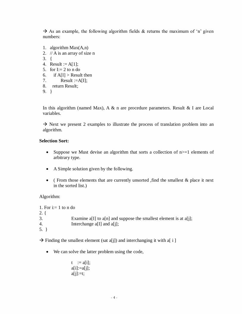
As an example, the following algorithm fields & returns the maximum of „n‟ given

numbers:

1. algorithm Max(A,n)

2. // A is an array of size n

3.

4. Result := A[1];

5. for I:= 2 to n do

6. if A[I] > Result then

7. Result :=A[I];

8. return Result;

9.

In this algorithm (named Max), A & n are procedure parameters. Result & I are Local

variables.

Next we present 2 examples to illustrate the process of translation problem into an

algorithm.

Selection Sort:

Suppose we Must devise an algorithm that sorts a collection of n>=1 elements of

arbitrary type.

A Simple solution given by the following.

( From those elements that are currently unsorted ,find the smallest & place it next

in the sorted list.)

Algorithm:

1. For i:= 1 to n do

2.

3. Examine a[I] to a[n] and suppose the smallest element is at a[j];

4. Interchange a[I] and a[j];

5.

Finding the smallest element (sat a[j]) and interchanging it with a[ i ]

We can solve the latter problem using the code,

t := a[i];

a[i]:=a[j];

a[j]:=t;

- 5 -

The first subtask can be solved by assuming the minimum is a[ I ];checking a[I]

with a[I+1],a[I+2]…….,and whenever a smaller element is found, regarding it as

the new minimum. a[n] is compared with the current minimum.

Putting all these observations together, we get the algorithm Selection sort.

Theorem:

Algorithm selection sort(a,n) correctly sorts a set of n>=1 elements .The result remains

is a a[1:n] such that a[1] <= a[2] ….<=a[n].

Selection Sort:

Selection Sort begins by finding the least element in the list. This element is

moved to the front. Then the least element among the remaining element is found out and put

into second position. This procedure is repeated till the entire list has been studied.

Example:

LIST L = 3,5,4,1,2

1 is selected , 1,5,4,3,2

2 is selected, 1,2,4,3,5



Proof:

We first note that any I, say I=q, following the execution of lines 6 to 9,it is the

case that a[q] Þ a[r],q<r<=n.

Also observe that when „i‟ becomes greater than q, a[1:q] is unchanged. Hence,

following the last execution of these lines (i.e. I=n).We have a[1] <= a[2]

<=……a[n].

We observe this point that the upper limit of the for loop in the line 4 can be

changed to n-1 without damaging the correctness of the algorithm.

Algorithm:

1. Algorithm selection sort (a,n)

2. // Sort the array a[1:n] into non-decreasing order.

3.

4. for I:=1 to n do

5.

6. j:=I;

7. for k:=i+1 to n do

8. if (a[k]<a[j])

9. t:=a[I];

10. a[I]:=a[j];

11. a[j]:=t;

- 6 -

12.

13.

Recursive Algorithms:

A Recursive function is a function that is defined in terms of itself.

Similarly, an algorithm is said to be recursive if the same algorithm is invoked in

the body.

An algorithm that calls itself is Direct Recursive.

Algorithm „A‟ is said to be Indirect Recursive if it calls another algorithm which

in turns calls „A‟.

The Recursive mechanism, are externally powerful, but even more importantly,

many times they can express an otherwise complex process very clearly. Or these

reasons we introduce recursion here.

The following 2 examples show how to develop a recursive algorithms.

In the first, we consider the Towers of Hanoi problem, and in the

second, we generate all possible permutations of a list of characters.

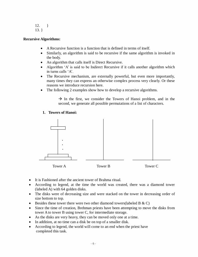
1. Towers of Hanoi:

.

.

.

Tower A Tower B Tower C

It is Fashioned after the ancient tower of Brahma ritual.

According to legend, at the time the world was created, there was a diamond tower

(labeled A) with 64 golden disks.

The disks were of decreasing size and were stacked on the tower in decreasing order of

size bottom to top.

Besides these tower there were two other diamond towers(labeled B & C)

Since the time of creation, Brehman priests have been attempting to move the disks from

tower A to tower B using tower C, for intermediate storage.

As the disks are very heavy, they can be moved only one at a time.

In addition, at no time can a disk be on top of a smaller disk.

According to legend, the world will come to an end when the priest have

completed this task.

- 7 -

A very elegant solution results from the use of recursion.

Assume that the number of disks is „n‟.

To get the largest disk to the bottom of tower B, we move the remaining „n-1‟

disks to tower C and then move the largest to tower B.

Now we are left with the tasks of moving the disks from tower C to B.

To do this, we have tower A and B available.

The fact, that towers B has a disk on it can be ignored as the disks larger than the

disks being moved from tower C and so any disk scan be placed on top of it.

Algorithm:

1. Algorithm TowersofHanoi(n,x,y,z)

2. //Move the top „n‟ disks from tower x to tower y.

3.

.

.

.

4.if(n>=1) then

5.

6. TowersofHanoi(n-1,x,z,y);

7. Write(“move top disk from tower “ X ,”to top of tower “ ,Y);

8. Towersofhanoi(n-1,z,y,x);

9.

10.

2. Permutation Generator:

Given a set of n>=1elements, the problem is to print all possible permutations of this

set.

For example, if the set is a,b,c ,then the set of permutation is,

(a,b,c),(a,c,b),(b,a,c),(b,c,a),(c,a,b),(c,b,a)

It is easy to see that given „n‟ elements there are n! different permutations.

A simple algorithm can be obtained by looking at the case of 4 statement(a,b,c,d)

The Answer can be constructed by writing

1. a followed by all the permutations of (b,c,d)

2. b followed by all the permutations of(a,c,d)

3. c followed by all the permutations of (a,b,d)

4. d followed by all the permutations of (a,b,c)

Algorithm:

Algorithm perm(a,k,n)

- 8 -

if(k=n) then write (a[1:n]); // output permutation

else //a[k:n] ahs more than one permutation

// Generate this recursively.

for I:=k to n do

t:=a[k];

a[k]:=a[I];

a[I]:=t;

perm(a,k+1,n);

//all permutation of a[k+1:n]

t:=a[k];

a[k]:=a[I];

a[I]:=t;

Performance Analysis:

1. Space Complexity:

The space complexity of an algorithm is the amount of money it needs to run

to compilation.

2. Time Complexity:

The time complexity of an algorithm is the amount of computer time it needs

to run to compilation.

Space Complexity:

Space Complexity Example:

Algorithm abc(a,b,c)

return a+b++*c+(a+b-c)/(a+b) +4.0;

The Space needed by each of these algorithms is seen to be the sum of the following

component.

1.A fixed part that is independent of the characteristics (eg:number,size)of the inputs and

outputs.

The part typically includes the instruction space (ie. Space for the code), space for simple

variable and fixed-size component variables (also called aggregate) space for constants, and

so on.

2. A variable part that consists of the space needed by component variables whose size is

dependent on the particular problem instance being solved, the space needed by

- 9 -

referenced variables (to the extent that is depends on instance characteristics), and the

recursion stack space.

The space requirement s(p) of any algorithm p may therefore be written as,

S(P) = c+ Sp(Instance characteristics)

Where „c‟ is a constant.

Example 2:

Algorithm sum(a,n)

s=0.0;

for I=1 to n do

s= s+a[I];

return s;

The problem instances for this algorithm are characterized by n,the number of

elements to be summed. The space needed d by „n‟ is one word, since it is of

type integer.

The space needed by „a‟a is the space needed by variables of tyepe array of

floating point numbers.

This is atleast „n‟ words, since „a‟ must be large enough to hold the „n‟

elements to be summed.

So,we obtain Ssum(n)>=(n+s)

[ n for a[],one each for n,I a& s]

Time Complexity:

The time T(p) taken by a program P is the sum of the compile time and the

run time(execution time)

The compile time does not depend on the instance characteristics. Also we may

assume that a compiled program will be run several times without recompilation .This

rum time is denoted by tp(instance characteristics).

The number of steps any problem statemn t is assigned depends on the kind of

statement.

For example, comments 0 steps.

Assignment statements 1 steps.

[Which does not involve any calls to other algorithms]

Interactive statement such as for, while & repeat-until Control part of the statement.

- 10 -

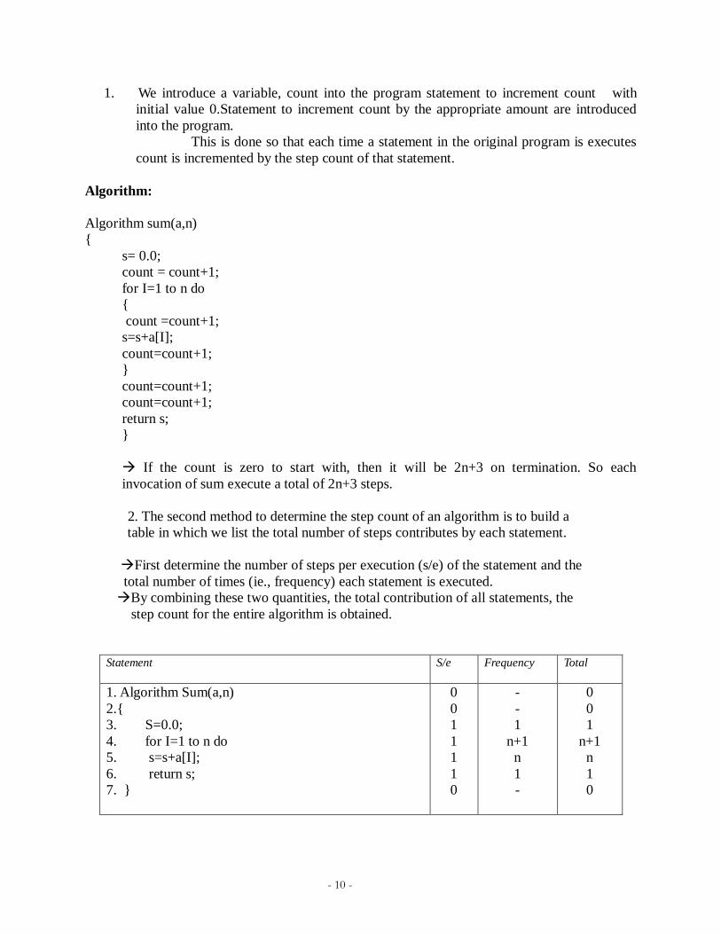
1. We introduce a variable, count into the program statement to increment count with

initial value 0.Statement to increment count by the appropriate amount are introduced

into the program.

This is done so that each time a statement in the original program is executes

count is incremented by the step count of that statement.

Algorithm:

Algorithm sum(a,n)

s= 0.0;

count = count+1;

for I=1 to n do

count =count+1;

s=s+a[I];

count=count+1;

count=count+1;

count=count+1;

return s;

If the count is zero to start with, then it will be 2n+3 on termination. So each

invocation of sum execute a total of 2n+3 steps.

2. The second method to determine the step count of an algorithm is to build a

table in which we list the total number of steps contributes by each statement.

First determine the number of steps per execution (s/e) of the statement and the

total number of times (ie., frequency) each statement is executed.

By combining these two quantities, the total contribution of all statements, the

step count for the entire algorithm is obtained.

Statement S/e Frequency Total

1. Algorithm Sum(a,n)

2.

3. S=0.0;

4. for I=1 to n do

5. s=s+a[I];

6. return s;

7.

0

0

1

1

1

1

0

-

-

1

n+1

n

1

-

0

0

1

n+1

n

1

0

- 11 -

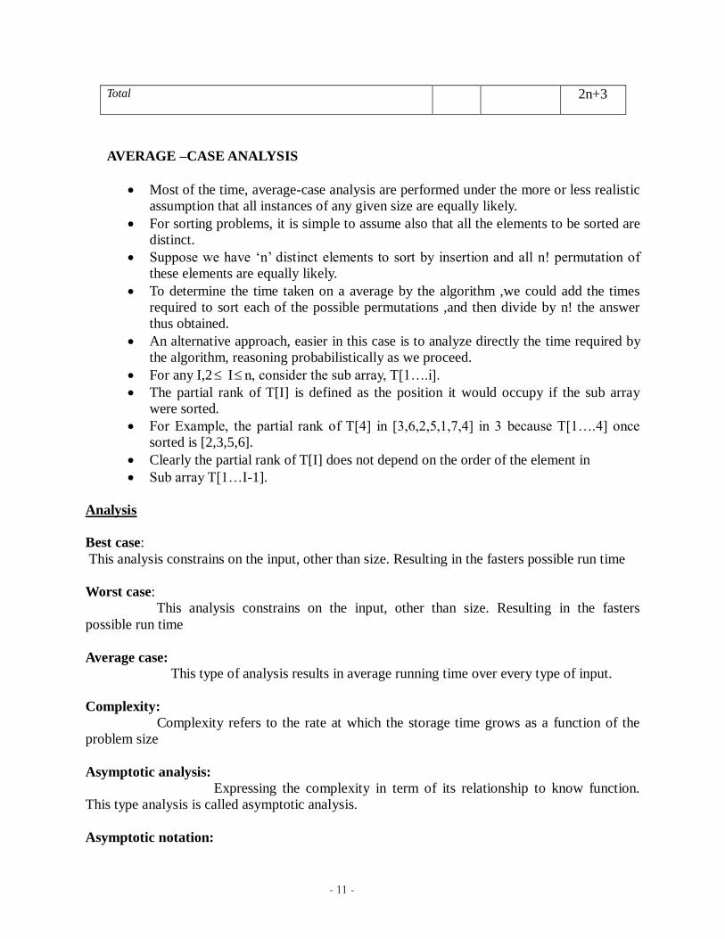
Total 2n+3

AVERAGE –CASE ANALYSIS

Most of the time, average-case analysis are performed under the more or less realistic

assumption that all instances of any given size are equally likely.

For sorting problems, it is simple to assume also that all the elements to be sorted are

distinct.

Suppose we have „n‟ distinct elements to sort by insertion and all n! permutation of

these elements are equally likely.

To determine the time taken on a average by the algorithm ,we could add the times

required to sort each of the possible permutations ,and then divide by n! the answer

thus obtained.

An alternative approach, easier in this case is to analyze directly the time required by

the algorithm, reasoning probabilistically as we proceed.

For any I,2 I n, consider the sub array, T[1….i].

The partial rank of T[I] is defined as the position it would occupy if the sub array

were sorted.

For Example, the partial rank of T[4] in [3,6,2,5,1,7,4] in 3 because T[1….4] once

sorted is [2,3,5,6].

Clearly the partial rank of T[I] does not depend on the order of the element in

Sub array T[1…I-1].

Analysis

Best case:

This analysis constrains on the input, other than size. Resulting in the fasters possible run time

Worst case:

This analysis constrains on the input, other than size. Resulting in the fasters

possible run time

Average case:

This type of analysis results in average running time over every type of input.

Complexity:

Complexity refers to the rate at which the storage time grows as a function of the

problem size

Asymptotic analysis:

Expressing the complexity in term of its relationship to know function.

This type analysis is called asymptotic analysis.

Asymptotic notation:

- 12 -

Big ‘oh’: the function f(n)=O(g(n)) iff there exist positive constants c and no such that

f(n)≤c*g(n) for all n, n ≥ no.

Omega: the function f(n)=Ω(g(n)) iff there exist positive constants c and no such that f(n) ≥

c*g(n) for all n, n ≥ no.

Theta: the function f(n)=ө(g(n)) iff there exist positive constants c1,c2 and no such that c1 g(n)

≤ f(n) ≤ c2 g(n) for all n, n ≥ no.

Recursion:

Recursion may have the following definitions:

-The nested repetition of identical algorithm is recursion.

-It is a technique of defining an object/process by itself.

-Recursion is a process by which a function calls itself repeatedly until some specified condition

has been satisfied.

When to use recursion:

Recursion can be used for repetitive computations in which each action is stated in terms

of previous result. There are two conditions that must be satisfied by any recursive procedure.

1. Each time a function calls itself it should get nearer to the solution.

2. There must be a decision criterion for stopping the process.

In making the decision about whether to write an algorithm in recursive or non-recursive form, it

is always advisable to consider a tree structure for the problem. If the structure is simple then use

non-recursive form. If the tree appears quite bushy, with little duplication of tasks, then recursion

is suitable.

The recursion algorithm for finding the factorial of a number is given below,

Algorithm : factorial-recursion

Input : n, the number whose factorial is to be found.

Output : f, the factorial of n

Method : if(n=0)

f=1

else

f=factorial(n-1) * n

if end

algorithm ends.

The general procedure for any recursive algorithm is as follows,

1. Save the parameters, local variables and return addresses.

- 13 -

2. If the termination criterion is reached perform final computation and goto step 3

otherwise perform final computations and goto step 1

3. Restore the most recently saved parameters, local variable and return address and goto

the latest return address.

Iteration v/s Recursion:

Demerits of recursive algorithms:

1. Many programming languages do not support recursion; hence, recursive mathematical

function is implemented using iterative methods.

2. Even though mathematical functions can be easily implemented using recursion it is

always at the cost of execution time and memory space. For example, the recursion tree

for generating 6 numbers in a Fibonacci series generation is given in fig 2.5. A Fibonacci

series is of the form 0,1,1,2,3,5,8,13,…etc, where the third number is the sum of

preceding two numbers and so on. It can be noticed from the fig 2.5 that, f(n-2) is

computed twice, f(n-3) is computed thrice, f(n-4) is computed 5 times.

3. A recursive procedure can be called from within or outside itself and to ensure its proper

functioning it has to save in some order the return addresses so that, a return to the proper

location will result when the return to a calling statement is made.

4. The recursive programs needs considerably more storage and will take more time.

Demerits of iterative methods :

Mathematical functions such as factorial and Fibonacci series generation can be easily

implemented using recursion than iteration.

In iterative techniques looping of statement is very much necessary.

Recursion is a top down approach to problem solving. It divides the problem into pieces or

selects out one key step, postponing the rest.

- 14 -

Iteration is more of a bottom up approach. It begins with what is known and from this constructs

the solution step by step. The iterative function obviously uses time that is O(n) where as

recursive function has an exponential time complexity.

It is always true that recursion can be replaced by iteration and stacks. It is also true that stack

can be replaced by a recursive program with no stack.

SOLVING RECURRENCES :-( Happen again (or) repeatedly)

The indispensable last step when analyzing an algorithm is often to solve a recurrence

equation.

With a little experience and intention, most recurrence can be solved by intelligent

guesswork.

However, there exists a powerful technique that can be used to solve certain classes of

recurrence almost automatically.

This is a main topic of this section the technique of the characteristic equation.

1. Intelligent guess work:

This approach generally proceeds in 4 stages.

1. Calculate the first few values of the recurrence

2. Look for regularity.

3. Guess a suitable general form.

4. And finally prove by mathematical induction(perhaps constructive induction).

Then this form is correct.

Consider the following recurrence,

0 if n=0

T(n) = 3T(n ÷ 2)+n otherwise

First step is to replace n ÷ 2 by n/2

- 15 -

It is tempting to restrict „n‟ to being ever since in that case n†2 = n/2, but recursively

dividing an even no. by 2, may produce an odd no. larger than 1.

Therefore, it is a better idea to restrict „n‟ to being an exact power of 2.

First, we tabulate the value of the recurrence on the first few powers of 2.

n 1 2 4 8 16 32

T(n) 1 5 19 65 211 665

* For instance, T(16) = 3 * T(8) +16

= 3 * 65 +16

= 211.

* Instead of writing T(2) = 5, it is more

useful to write T(2) = 3 * 1 +2.

Then,

T(A) = 3 * T(2) +4

= 3 * (3 * 1 +2) +4

= (32 * 1) + (3 * 2) +4

* We continue in this way, writing „n‟ as an explicit power of 2.

n T(n)

1 1

2 3 * 1 +2

22 3

2 * 1 + 3 * 2 + 2

2

23 3

3 * 1 + 3

2 * 2 + 3 * 2

2 + 2

3

24 3

4 * 1 + 3

3 * 2 + 3

2 * 2

2 + 3 * 2

3 + 2

4

25 3

5 * 1 + 3

4 * 2 + 3

3 * 2

2 + 3

2 * 2

3 + 3 * 2

4 + 2

5

The pattern is now obvious.

T(2k ) = 3

k2

0 + 3

k-12

1 + 3

k-22

2+…+3

12

k-1 + 3

02

k.

= ∑ 3k-i

2i

= 3k ∑ (2/3)

i

= 3k * [(1 – (2/3)

k + 1) / (1 – (2/3)]

= 3k+1

– 2k+1

Proposition: (Geometric Series)

- 16 -

Let Sn be the sum of the first n terms of the geometric series a, ar, ar2….Then

Sn = a(1-rn)/(1-r), except in the special case when r = 1; when Sn = an.

= 3k * [ (1 – (2/3)

k+1) / (1 – (2/3))]

= 3k * [((3

k+1 – 2

k+1)/ 3

k+1) / ((3 – 2) / 3)]

3 k+1

– 2k+1

3

= 3k * ----------------- * ----

3 k+1

1

3 k+1

– 2k+

1

= 3k * -----------------

3k+1-1

= 3k+1

– 2k+1

* It is easy to check this formula against our earlier tabulation.

EG : 2

0 n=0

tn = 5 n=1

3tn-1 + 4tn-2, otherwise

tn = 3tn-1 – 4tn-2 = 0 General function

Characteristics Polynomial, x2 – 3x – 4 = 0

(x – 4)(x + 1) = 0

Roots r1 = 4, r2 = -1

General Solution, fn = C1r1n + C2 r2

n (A)

n=0 C1 + C2 = 0 (1)

n=1 C1r1 + C2r2 = 5 (2)

Eqn 1 C1 = -C2

sub C1 value in Eqn (2)

-C2r1 + C2r2 = 5

C2(r2 – r1) = 5

5

C2 = -------

- 17 -

r2 – r1

5

= ------

-1 + 4

= 5 / (-5) = -1

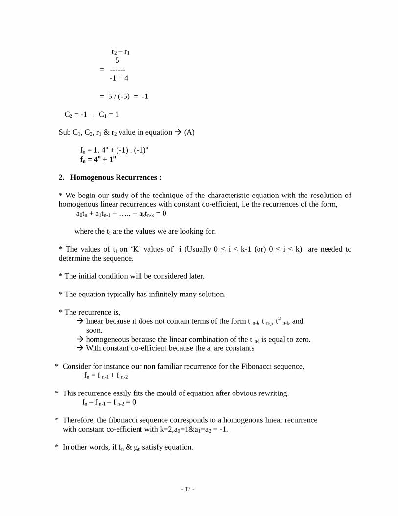
C2 = -1 , C1 = 1

Sub C1, C2, r1 & r2 value in equation (A)

fn = 1. 4n + (-1) . (-1)

n

fn = 4n + 1

n

2. Homogenous Recurrences :

* We begin our study of the technique of the characteristic equation with the resolution of

homogenous linear recurrences with constant co-efficient, i.e the recurrences of the form,

a0tn + a1tn-1 + ….. + aktn-k = 0

where the ti are the values we are looking for.

* The values of ti on „K‟ values of i (Usually 0 ≤ i ≤ k-1 (or) 0 ≤ i ≤ k) are needed to

determine the sequence.

* The initial condition will be considered later.

* The equation typically has infinitely many solution.

* The recurrence is,

linear because it does not contain terms of the form t n-i, t n-j, t2 n-i, and

soon.

homogeneous because the linear combination of the t n-i is equal to zero.

With constant co-efficient because the ai are constants

* Consider for instance our non familiar recurrence for the Fibonacci sequence,

fn = f n-1 + f n-2

* This recurrence easily fits the mould of equation after obvious rewriting.

fn – f n-1 – f n-2 = 0

* Therefore, the fibonacci sequence corresponds to a homogenous linear recurrence

with constant co-efficient with k=2,a0=1&a1=a2 = -1.

* In other words, if fn & gn satisfy equation.

- 18 -

k

So ∑ ai f n-i = 0 & similarly for gn & fn

i=0

We set tn = C fn + d gn for arbitrary constants C & d, then tn is also a solution to

equation.

* This is true because,

a0tn + a1tn-1 + … + aktn-k

= a0(C fn +d gn) + a1(C fn-1 + d gn-1) + …+ ak(C fn-k + d gn-k)

= C(a0 fn + a1 fn-1 + … + ak fn-k)+

d(a0 gn + a1 gn-1 + … + ak gn-k)

= C * 0 + d * 0

= 0.

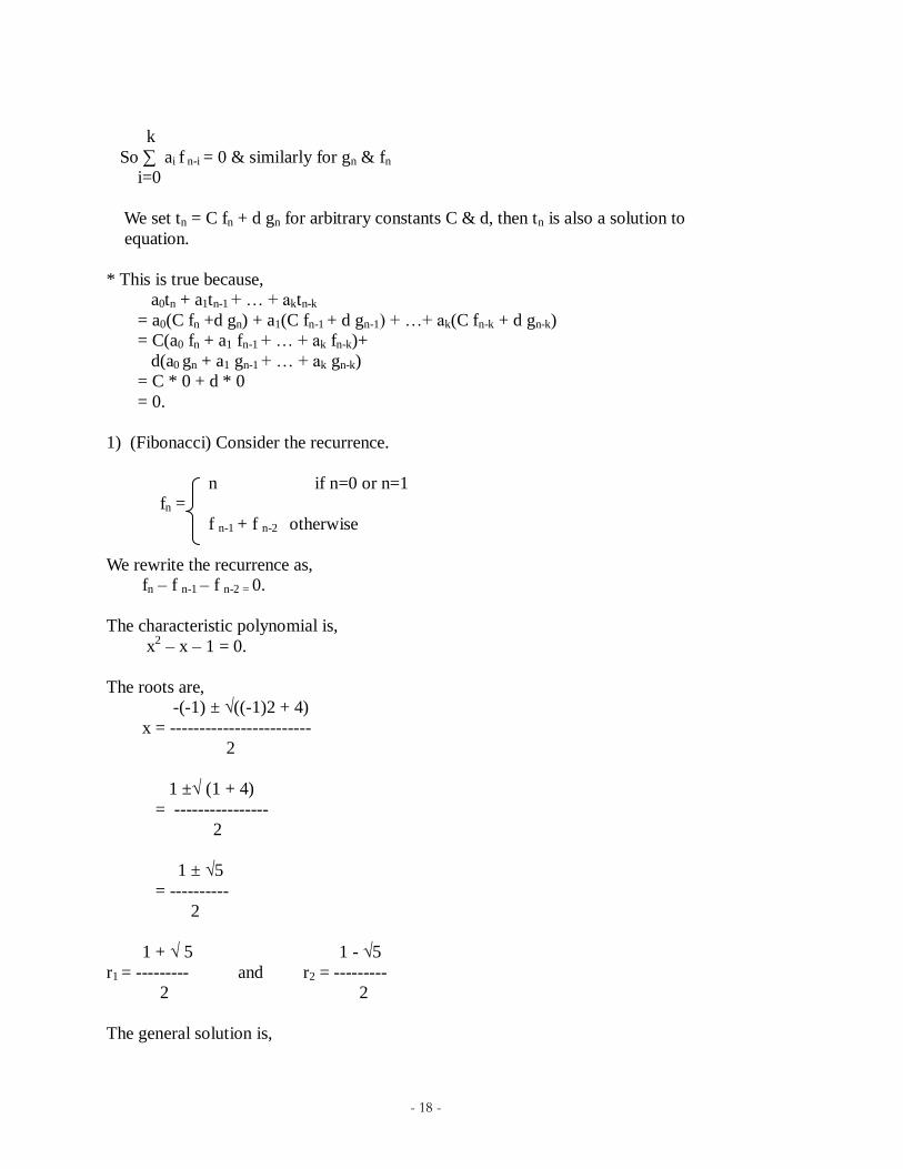
1) (Fibonacci) Consider the recurrence.

n if n=0 or n=1

fn =

f n-1 + f n-2 otherwise

We rewrite the recurrence as,

fn – f n-1 – f n-2 = 0.

The characteristic polynomial is,

x2 – x – 1 = 0.

The roots are,

-(-1) ± √((-1)2 + 4)

x = ------------------------

2

1 ±√ (1 + 4)

= ----------------

2

1 ± √5

= ----------

2

1 + √ 5 1 - √5

r1 = --------- and r2 = ---------

2 2

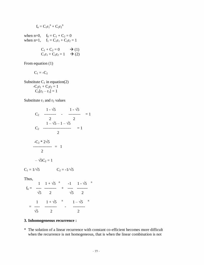
The general solution is,

- 19 -

fn = C1r1n + C2r2

n

when n=0, f0 = C1 + C2 = 0

when n=1, f1 = C1r1 + C2r2 = 1

C1 + C2 = 0 (1)

C1r1 + C2r2 = 1 (2)

From equation (1)

C1 = -C2

Substitute C1 in equation(2)

-C2r1 + C2r2 = 1

C2[r2 – r1] = 1

Substitute r1 and r2 values

1 - √5 1 - √5

C2 --------- - --------- = 1

2 2

1 – √5 – 1 – √5

C2 --------------------- = 1

2

-C2 * 2√5

-------------- = 1

2

– √5C2 = 1

C1 = 1/√5 C2 = -1/√5

Thus,

1 1 + √5 n -1 1 - √5

n

fn = ---- --------- + ---- --------

√5 2 √5 2

1 1 + √5 n 1 – √5

n

= ---- --------- - ---------

√5 2 2

3. Inhomogeneous recurrence :

* The solution of a linear recurrence with constant co-efficient becomes more difficult

when the recurrence is not homogeneous, that is when the linear combination is not

- 20 -

equal to zero.

* Consider the following recurrence

a0tn + a1 t n-1 + … + ak t n-k = bn p(n)

* The left hand side is the same as before,(homogeneous) but on the right-hand side

we have bnp(n), where,

b is a constant

p(n) is a polynomial in „n‟ of degree „d‟.

Example(1) :

Consider the recurrence,

tn – 2t n-1 = 3n (A)

In this case, b=3, p(n) = 1, degree = 0.


(x – 2)(x – 3) = 0

The roots are, r1 = 2, r2 = 3

The general solution,

tn = C1r1n + C2r2

n

tn = C12n + C23

n (1)

when n=0, C1 + C2 = t0 (2)

when n=1, 2C1 + 3C2 = t1 (3)

sub n=1 in eqn (A)

t1 – 2t0 = 3

t1 = 3 + 2t0

substitute t1 in eqn(3),

(2) * 2 2C1 + 2C2 = 2t0

2C1 + 3C2 = (3 + 2t0)

-------------------------------

-C2 = -3

C2 = 3

Sub C2 = 3 in eqn (2)

C1 + C2 = t0

C1 + 3 = t0

C1 = t0 – 3

Therefore tn = (t0-3)2n + 3. 3

n

= Max[O[(t0 – 3) 2n], O[3.3

n]]

- 21 -

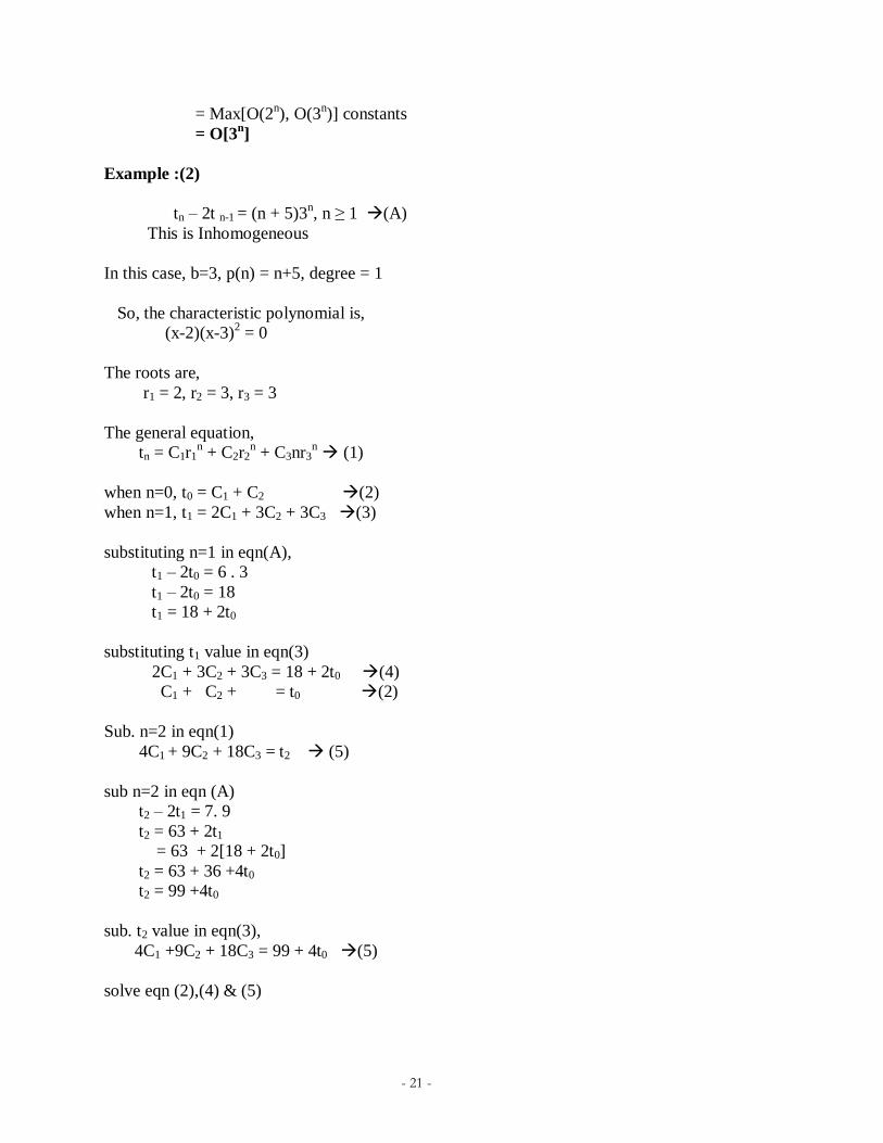
= Max[O(2n), O(3

n)] constants

= O[3n]

Example :(2)

tn – 2t n-1 = (n + 5)3n, n ≥ 1 (A)

This is Inhomogeneous

In this case, b=3, p(n) = n+5, degree = 1

So, the characteristic polynomial is,

(x-2)(x-3)2 = 0

The roots are,

r1 = 2, r2 = 3, r3 = 3

The general equation,

tn = C1r1n + C2r2

n + C3nr3

n (1)

when n=0, t0 = C1 + C2 (2)

when n=1, t1 = 2C1 + 3C2 + 3C3 (3)

substituting n=1 in eqn(A),

t1 – 2t0 = 6 . 3

t1 – 2t0 = 18

t1 = 18 + 2t0

substituting t1 value in eqn(3)

2C1 + 3C2 + 3C3 = 18 + 2t0 (4)

C1 + C2 + = t0 (2)

Sub. n=2 in eqn(1)

4C1 + 9C2 + 18C3 = t2 (5)

sub n=2 in eqn (A)

t2 – 2t1 = 7. 9

t2 = 63 + 2t1

= 63 + 2[18 + 2t0]

t2 = 63 + 36 +4t0

t2 = 99 +4t0

sub. t2 value in eqn(3),

4C1 +9C2 + 18C3 = 99 + 4t0 (5)

solve eqn (2),(4) & (5)

- 22 -

n=0, C1 + C2 = t0 (2)

n=1, 2C1 + 3C2 + 3C3 = 18 + 2t0 (4)

n=2, 4C1 + 9C2 + 18C3 = 99 + 4t0 (5)

(4) * 6 12C1 + 18C2 +18C3 = 108 + 2t0 (4)

(5) 4C1 + 9C2 + 18C3 = 99 + 4t0 (5)

------------------------------------------------

8C1 + 9C2 = 9 + 8t0 (6)

(2) * 8 8C1 + 8C2 = 8t0 (2)

(6) 8C1 + 9C2 = 9 +8t0 (6)

--------------------------

-C2 = -9

C2 = 9

Sub, C2 = 9 in eqn(2)

C1 + C2 = t0

C1 + 9 = t0

C1 = t0-9

Sub C1 & C2 in eqn (4)

2C1 + 3C2 + 3C3 = 18 + 2t0

2(t0-9) + 3(9) + 3C3 = 18 + 2t0

2t0 – 18 + 27 + 3C3 = 18 + 2t0

2t0 + 9 + 3C3 = 18 + 2t0

3C3 = 18 – 9 + 2t0 – 2t0

3C3 = 9

C3 = 9/3

C3 = 3

Sub. C1, C2, C3, r1, r2, r3 values in eqn (1)

tn = C12n + C23

n + C3.n.3

n

= (t0 – 9)2n + 9.3

n + 3.n.3

n

= Max[O[(t0-9),2n], O[9.3

n], O[3.n.3

n]]

= Max[O(2n), O(3

n), O(n3

n)]

tn = O[n3n]

Example: (3)


1 if n=0

tn =

4t n-1 – 2n otherwise

- 23 -

tn – 4t n-1 = -2n (A)

In this case , c=2, p(n) = -1, degree =0

(x-4)(x-2) = 0


The general solution ,

tn = C1r1n + C2r2

n

tn = C14n + C22

n (1)

when n=0, in (1) C1 + C2 = 1 (2)

when n=1, in (1) 4C1 + 2C2 = t1 (3)

sub n=1 in (A),

tn – 4t n-1 = -2n

t1 – 4t0 = -2

t1 = 4t0 – 2 [since t0 = 1]

t1 = 2

sub t1 value in eqn (3)

4C1 + 2C2 = 4t0 – 2 (3)

(2) * 4 4C1 + 4C2 = 4

----------------------------

-2C2 = 4t0 - 6

= 4(1) - 6

= -2

C2 = 1

-2C2 = 4t0 - 6

2C2 = 6 – 4t0

C2 = 3 – 2t0

3 – 2(1) = 1

C2 = 1

Sub. C2 value in eqn(2),

C1 + C2 = 1

C1 + (3-2t0) = 1

C1 + 3 – 2t0 = 1

C1 = 1 – 3 + 2t0

C1 = 2t0 - 2

= 2(1) – 2 = 0

C1 = 0

Sub C1 & C2 value in eqn (1)

tn = C14n + C22

n

- 24 -

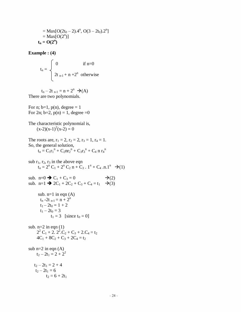
= Max[O(2t0 – 2).4n, O(3 – 2t0).2

n]

= Max[O(2n)]

tn = O(2n)

Example : (4)

0 if n=0

tn =

2t n-1 + n +2n otherwise

tn – 2t n-1 = n + 2n (A)

There are two polynomials.

For n; b=1, p(n), degree = 1

For 2n; b=2, p(n) = 1, degree =0


(x-2)(x-1)2(x-2) = 0

The roots are, r1 = 2, r2 = 2, r3 = 1, r4 = 1.

So, the general solution,

tn = C1r1n + C2nr2

n + C3r3

n + C4 n r4

n

sub r1, r2, r3 in the above eqn

tn = 2n C1 + 2

n C2 n + C3 . 1

n + C4 .n.1

n (1)

sub. n=0 C1 + C3 = 0 (2)

sub. n=1 2C1 + 2C2 + C3 + C4 = t1 (3)

sub. n=1 in eqn (A)

tn -2t n-1 = n + 2n

t1 – 2t0 = 1 + 2

t1 – 2t0 = 3

t1 = 3 [since t0 = 0]

sub. n=2 in eqn (1)

22 C1 + 2. 2

2.C2 + C3 + 2.C4 = t2

4C1 + 8C2 + C3 + 2C4 = t2

sub n=2 in eqn (A)

t2 – 2t1 = 2 + 22

t2 – 2t1 = 2 + 4

t2 – 2t1 = 6

t2 = 6 + 2t1

- 25 -

t2 = 6 + 2.3

t2 = 6 + 6

t2 = 12

4C1 + 8C2 + C3 + 2C4 = 12 (4)

sub n=3 in eqn (!)

23 C1 + 3.2

3.C2 + C3 + 3C4 = t3

3C1 + 24C2 + C3 + 3C4 = t3

sub n=3 in eqn (A)

t3 – 2t2 = 3 + 23

t3 – 2t2 = 3 + 8

t3 – 2(12) = 11

t3 – 24 = 11

t3 = 11 + 24

t3 = 35

8C1 + 24C2 + C3 + 3C4 = 35 (5)

n=0, solve; C1 + C3 = 0 (2)

n=1,(2), (3), (4)&(5) 2C1 + 2C2 + C3 + C4 = 3 (3)

n=2, 4C1 + 8C2 + C3 + 2C4 = 12 (4)

n=3, 8C1 + 24C2 + C3 + 3C4 = 35 (5)

---------------------------------------

-4C1 – 16C2 – C4 = -23 (6)

solve: (2) & (3)

(2) C1 + C3 = 0

(3) 2C1 + C3 + 2C2 + C4 = 3

---------------------------------

-C1 – 2C2 – C4 = -3 (7)

solve(6) & (7)

(6) -4C1 – 16C2 – C4 = -23

(7) -C1 – 2C2 – C4 = -3

---------------------------------

-3C1 – 14C2 = 20 (8)

4. Change of variables: * It is sometimes possible to solve more complicated recurrences by making a

change of variable.

* In the following example, we write T(n) for the term of a general recurrences,

and ti for the term of a new recurrence obtained from the first by a change of variable.

- 26 -

Example: (1)


1 , if n=1

T(n) =

3T(n/2) + n , if „n‟ is a power of 2, n>1

Reconsider the recurrence we solved by intelligent guesswork in the previous

section, but only for the case when „n‟ is a power of 2

1

T(n) =

3T(n/2) + n

* We replace „n‟ by 2i.

* This is achieved by introducing new recurrence ti, define by ti = T(2i)

* This transformation is useful because n/2 becomes (2i)/2 = 2

i-1

* In other words, our original recurrence in which T(n) is defined as a function of

T(n/2) given way to one in which ti is defined as a function of t i-1, precisely

the type of recurrence we have learned to solve.

ti = T(2i) = 3T(2

i-1) + 2

i

ti = 3t i-1 + 2i

ti – 3t i-1 = 2i (A)

In this case,

b = 2, p(n) = 1, degree = 0

So, the characteristic equation,

(x – 3)(x – 2) = 0

The roots are, r1 = 3, r2 = 2.

The general equation,

tn = C1 r1i + C2 r2

i

sub. r1 & r2: tn = 3nC1 + C2 2

n

tn = C1 3i + C2 2

i

We use the fact that, T(2i) = ti & thus T(n) = tlogn when n= 2

i to obtain,

T(n) = C1. 3 log

2n + C2. 2

log2

n

T(n) = C1 . nlog

23 + C2.n [i = logn]

When „n‟ is a power of 2, which is sufficient to conclude that,

T(n) = O(n log3

) ‘n’ is a power of 2

Example: (2)

- 27 -


T(n) = 4T(n/2) + n2 (A)

Where „n‟ is a power of 2, n ≥ 2.

ti = T(2i) = 4T(2

i-1) + (2

i)2

ti = 4t i-1 + 4i

ti – 4t i-1 = 4i

In this eqn,

b = 4, P(n) = 1, degree = 0

The characteristic polynomial,

(x – 4)(x – 4) = 0

The roots are, r1 = 4, r2 = 4.

So, the general equation,

ti = C14i + C24

i.i [since i = logn]

= C1 4 log n

+ C2. 4 logn

. logn [since 2i = n]

= C1 . n log 4

+ C2. n log4

.n log1

T(n) = O(n log4

) ‘n’ is the power of 2.

EXAMPLE : 3

T(n) = 2T(n/2) + n logn

When „n‟ is a power of 2, n ≥ 2

ti = T(2i) = 2T(2

i/2) + 2

i .i [since 2

i = n; i =logn]

ti – 2t i-1 = i. 2i

In this case,

b = 2, P(n) = i, degree = 1

(x – 2)(x – 2)2 = 0

The roots are, r1 = 2, r2 = 2, r3 = 2

The general solution is,

tn = C12i + C2. 2

i . i + C3. i

2. 2

i

= nC1 + nC2 + nC3(log n2

2n)

tn = O(n.log2

2n)

Example: 4

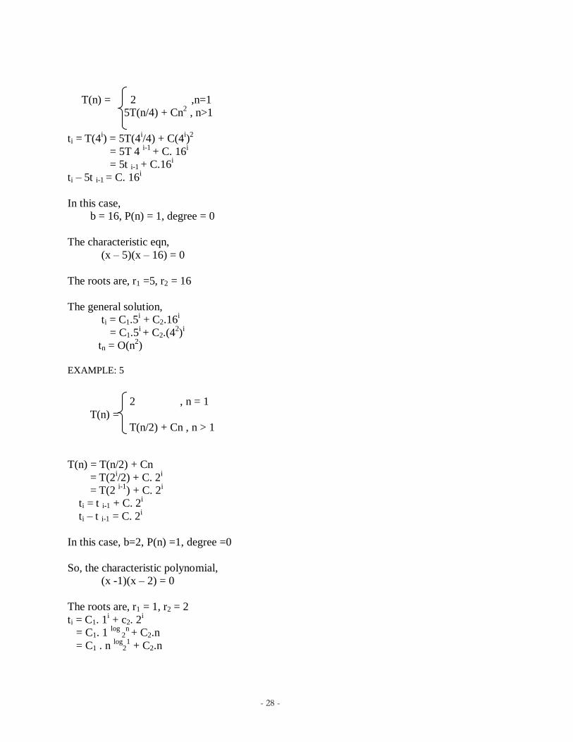
- 28 -

T(n) = 2 ,n=1

5T(n/4) + Cn2 , n>1

ti = T(4i) = 5T(4

i/4) + C(4

i)2

= 5T 4 i-1

+ C. 16i

= 5t i-1 + C.16i

ti – 5t i-1 = C. 16i

In this case,

b = 16, P(n) = 1, degree = 0

The characteristic eqn,

(x – 5)(x – 16) = 0

The roots are, r1 =5, r2 = 16

The general solution,

ti = C1.5i + C2.16

i

= C1.5i + C2.(4

2)

i

tn = O(n2)

EXAMPLE: 5

2 , n = 1

T(n) =

T(n/2) + Cn , n > 1

T(n) = T(n/2) + Cn

= T(2i/2) + C. 2

i

= T(2 i-1

) + C. 2i

ti = t i-1 + C. 2i

ti – t i-1 = C. 2i

In this case, b=2, P(n) =1, degree =0

So, the characteristic polynomial,

(x -1)(x – 2) = 0


ti = C1. 1i + c2. 2

i

= C1. 1 log

2n + C2.n

= C1 . n log

21 + C2.n

- 29 -

tn = O(n)

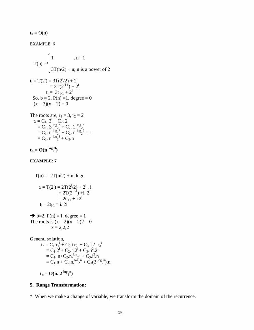
EXAMPLE: 6

1 , n =1

T(n) =

3T(n/2) + n; n is a power of 2

ti = T(2i) = 3T(2

i/2) + 2

i

= 3T(2 i-1

) + 2i

ti = 3t i-1 + 2i

So, b = 2, P(n) =1, degree = 0

(x – 3)(x – 2) = 0


ti = C1. 3i + C2. 2

i

= C1. 3 log

2n + C2. 2

log2

n

= C1. n log

23 + C2. n

log2

2 = 1

= C1. n log

23 + C2.n

tn = O(n log

23)

EXAMPLE: 7

T(n) = 2T(n/2) + n. logn

ti = T(2i) = 2T(2

i/2) + 2

i . i

= 2T(2 i-1

) +i. 2i

= 2t i-1 + i.2i

ti – 2ti-1 = i. 2i

b=2, P(n) = I, degree = 1

The roots is (x – 2)(x – 2)2 = 0

x = 2,2,2

General solution,

tn = C1.r1i + C2.i.r2

i + C3. i2. r3

i

= C1.2i + C2. i.2

i + C3. i

2.2

i

= C1. n+C2.n.log

2n + C3.i

2.n

= C1.n + C2.n.log

2n + C3(2

log2

n).n

tn = O(n. 2 log

2n)

5. Range Transformation:

* When we make a change of variable, we transform the domain of the recurrence.

- 30 -

* Instead it may be useful to transform the range to obtain a recurrence in a form

that we know how to solve

* Both transformation can be sometimes be used together.

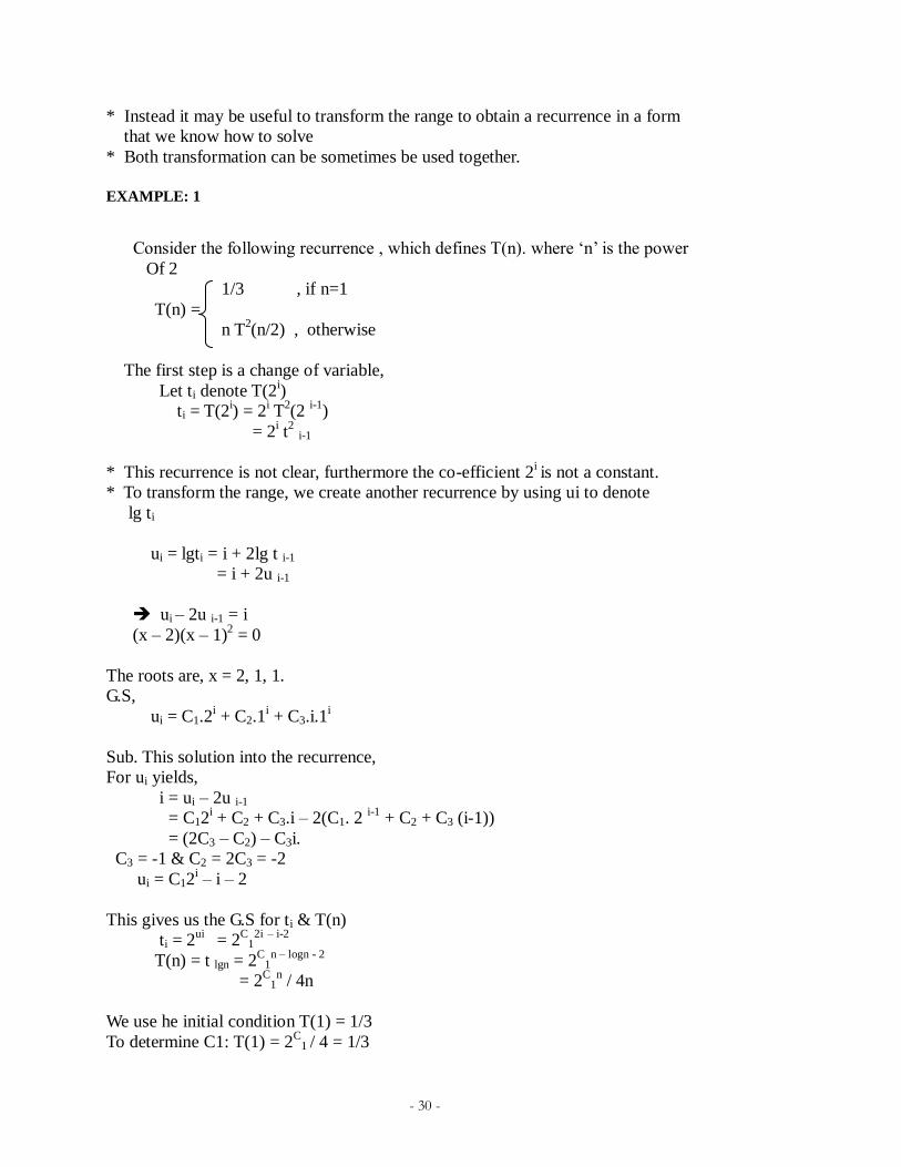
EXAMPLE: 1

Consider the following recurrence , which defines T(n). where „n‟ is the power

Of 2

1/3 , if n=1

T(n) =

n T2(n/2) , otherwise

The first step is a change of variable,

Let ti denote T(2i)

ti = T(2i) = 2

i T

2(2

i-1)

= 2i t

2 i-1

* This recurrence is not clear, furthermore the co-efficient 2i is not a constant.

* To transform the range, we create another recurrence by using ui to denote

lg ti

ui = lgti = i + 2lg t i-1

= i + 2u i-1

ui – 2u i-1 = i

(x – 2)(x – 1)2 = 0

The roots are, x = 2, 1, 1.

G.S,

ui = C1.2i + C2.1

i + C3.i.1

i

Sub. This solution into the recurrence,

For ui yields,

i = ui – 2u i-1

= C12i + C2 + C3.i – 2(C1. 2

i-1 + C2 + C3 (i-1))

= (2C3 – C2) – C3i.

C3 = -1 & C2 = 2C3 = -2

ui = C12i – i – 2

This gives us the G.S for ti & T(n)

ti = 2ui = 2

C1

2i – i-2

T(n) = t lgn = 2C

1n – logn - 2

= 2C

1n / 4n

We use he initial condition T(1) = 1/3

To determine C1: T(1) = 2C

1 / 4 = 1/3

- 31 -

Implies that C1 = lg(4/3) = 2 – log 3

The final solution is

T(n) = 2 2n

/ 4n 3n

1. Newton Raphson method: x2= x1-f(x1)/f1(x1)

SEARCHING

Let us assume that we have a sequential file and we wish to retrieve an element matching

with key „k‟, then, we have to search the entire file from the beginning till the end to check

whether the element matching k is present in the file or not.

There are a number of complex searching algorithms to serve the purpose of searching. The

linear search and binary search methods are relatively straight forward methods of searching.

Sequential search:

In this method, we start to search from the beginning of the list and examine each

element till the end of the list. If the desired element is found we stop the search and return the

index of that element. If the item is not found and the list is exhausted the search returns a zero

value.

In the worst case the item is not found or the search item is the last (nth) element. For both

situations we must examine all n elements of the array so the order of magnitude or complexity

of the sequential search is n. i.e., O(n). The execution time for this algorithm is proportional to n

that is the algorithm executes in linear time.

The algorithm for sequential search is as follows,

Algorithm : sequential search

Input : A, vector of n elements

K, search element

Output : j –index of k

Method : i=1

While(i<=n)

if(A[i]=k)

write("search successful")

write(k is at location i)

exit();

else

i++

if end

- 32 -

while end

write (search unsuccessful);

algorithm ends.

Binary search:

Binary search method is also relatively simple method. For this method it is necessary to

have the vector in an alphabetical or numerically increasing order. A search for a particular item

with X resembles the search for a word in the dictionary. The approximate mid entry is located

and its key value is examined. If the mid value is greater than X, then the list is chopped off at

the (mid-1)th

location. Now the list gets reduced to half the original list. The middle entry of the

left-reduced list is examined in a similar manner. This procedure is repeated until the item is

found or the list has no more elements. On the other hand, if the mid value is lesser than X, then

the list is chopped off at (mid+1)th

location. The middle entry of the right-reduced list is

examined and the procedure is continued until desired key is found or the search interval is

exhausted.

The algorithm for binary search is as follows,

Algorithm : binary search

Input : A, vector of n elements

K, search element

Output : low –index of k

Method : low=1,high=n

While(low<=high-1)

mid=(low+high)/2

if(k<a[mid])

high=mid

else

low=mid

if end

while end

if(k=A[low])

write("search successful")

write(k is at location low)

exit();

else

write (search unsuccessful);

if end;

algorithm ends.

- 33 -

SORTING

One of the major applications in computer science is the sorting of information in a table.

Sorting algorithms arrange items in a set according to a predefined ordering relation. The most

common types of data are string information and numerical information. The ordering relation

for numeric data simply involves arranging items in sequence from smallest to largest and from

largest to smallest, which is called ascending and descending order respectively.

The items in a set arranged in non-decreasing order are 7,11,13,16,16,19,23. The items in a set

arranged in descending order is of the form 23,19,16,16,13,11,7

Similarly for string information, a, abacus, above, be, become, beyondis in ascending order

and beyond, become, be, above, abacus, ais in descending order.

There are numerous methods available for sorting information. But, not even one of them is best

for all applications. Performance of the methods depends on parameters like, size of the data set,

degree of relative order already present in the data etc.

Selection sort :

The idea in selection sort is to find the smallest value and place it in an order, then find

the next smallest and place in the right order. This process is continued till the entire table is

sorted.

Consider the unsorted array,

a[1] a[2] a[8]

20 35 18 8 14 41 3 39

The resulting array should be

a[1] a[2] a[8]

3 8 14 18 20 35 39 41

One way to sort the unsorted array would be to perform the following steps:

Find the smallest element in the unsorted array

Place the smallest element in position of a[1]

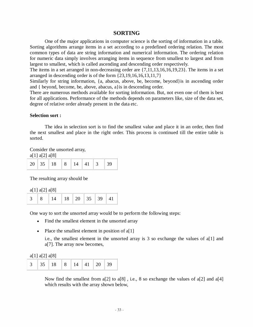
i.e., the smallest element in the unsorted array is 3 so exchange the values of a[1] and

a[7]. The array now becomes,

a[1] a[2] a[8]

3 35 18 8 14 41 20 39

Now find the smallest from a[2] to a[8] , i.e., 8 so exchange the values of a[2] and a[4]

which results with the array shown below,

- 34 -

a[1] a[2] a[8]

3 8 18 35 14 41 20 39

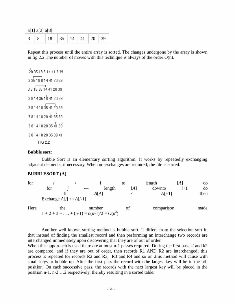
Repeat this process until the entire array is sorted. The changes undergone by the array is shown

in fig 2.2.The number of moves with this technique is always of the order O(n).

Bubble sort:

Bubble Sort is an elementary sorting algorithm. It works by repeatedly exchanging

adjacent elements, if necessary. When no exchanges are required, the file is sorted.

BUBBLESORT (A)

for i ← 1 to length [A] do

for j ← length [A] downto i+1 do

If A[A] < A[j-1] then

Exchange A[j] ↔ A[j-1]

Here the number of comparison made

1 + 2 + 3 + . . . + (n-1) = n(n-1)/2 = O(n2)

Another well known sorting method is bubble sort. It differs from the selection sort in

that instead of finding the smallest record and then performing an interchange two records are

interchanged immediately upon discovering that they are of out of order.

When this apporoach is used there are at most n-1 passes required. During the first pass k1and k2

are compared, and if they are out of order, then records R1 AND R2 are interchanged; this

process is repeated for records R2 and R3, R3 and R4 and so on .this method will cause with

small keys to bubble up. After the first pass the record with the largest key will be in the nth

position. On each successive pass, the records with the next largest key will be placed in the

position n-1, n-2 …2 respectively, thereby resulting in a sorted table.

- 35 -

After each pass through the table, a check can be made to determine whether any

interchanges were made during that pass. If no interchanges occurred then the table must be

sorted and no further passes are required.

Insertion sort :

Insertion sort is a straight forward method that is useful for small collection of data. The

idea here is to obtain the complete solution by inserting an element from the unordered part into

the partially ordered solution extending it by one element. Selecting an element from the

unordered list could be simple if the first element of that list is selected.

a[1] a[2] a[8]

20 35 18 8 14 41 3 39

Initially the whole array is unordered. So select the minimum and put it in place of a[1] to

act as sentinel. Now the array is of the form,

a[1] a[2] a[8]

3 35 18 8 14 41 20 39

Now we have one element in the sorted list and the remaining elements are in the unordered set.

Select the next element to be inserted. If the selected element is less than the preceding element

move the preceding element by one position and insert the smaller element.

In the above array the next element to be inserted is x=35, but the preceding element is 3 which

is less than x. Hence, take the next element for insertion i.e., 18. 18 is less than 35, so move 35

one position ahead and place 18 at that place. The resulting array will be,

a[1] a[2] a[8]

3 18 35 8 14 41 20 39

Now the element to be inserted is 8. 8 is less than 35 and 8 is also less than 18 so move

35 and 18 one position right and place 8 at a[2]. This process is carried till the sorted array is

obtained.

- 36 -

The changes undergone are shown in fig 2.3.

One of the disadvantages of the insertion sort method is the amount of movement of data. In the

worst case, the number of moves is of the order O(n2). For lengthy records it is quite time

consuming.

Heaps and Heap sort:

A heap is a complete binary tree with the property that the value at each node is atleast as

large as the value at its children.

The definition of a max heap implies that one of the largest elements is at the root of the heap. If

the elements are distinct then the root contains the largest item. A max heap can be implemented

using an array an[ ].

To insert an element into the heap, one adds it "at the bottom" of the heap and then

compares it with its parent, grandparent, great grandparent and so on, until it is less than or equal

to one of these values. Algorithm insert describes this process in detail.

Algorithm Insert(a,n)

// Insert a[n] into the heap which is stored in a[1:n-1]

I=n;

item=a[n];

while( (I>n) and (a[ I!/2 ] < item)) do

a[I] = a[I/2];

I=I/2;

a[I]=item;

return (true);

- 37 -

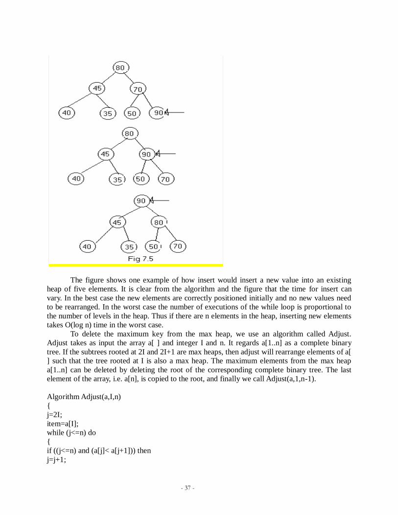
The figure shows one example of how insert would insert a new value into an existing

heap of five elements. It is clear from the algorithm and the figure that the time for insert can

vary. In the best case the new elements are correctly positioned initially and no new values need

to be rearranged. In the worst case the number of executions of the while loop is proportional to

the number of levels in the heap. Thus if there are n elements in the heap, inserting new elements

takes O(log n) time in the worst case.

To delete the maximum key from the max heap, we use an algorithm called Adjust.

Adjust takes as input the array a[ ] and integer I and n. It regards a[1..n] as a complete binary

tree. If the subtrees rooted at 2I and 2I+1 are max heaps, then adjust will rearrange elements of a[

] such that the tree rooted at I is also a max heap. The maximum elements from the max heap

a[1..n] can be deleted by deleting the root of the corresponding complete binary tree. The last

element of the array, i.e. a[n], is copied to the root, and finally we call Adjust(a,1,n-1).

Algorithm Adjust(a,I,n)

j=2I;

item=a[I];

while (j<=n) do

if ((j<=n) and (a[j]< a[j+1])) then

j=j+1;

- 38 -

//compare left and right child and let j be the right

//child

if ( item >= a[I]) then break;

// a position for item is found

a[i/2]=a[j];

j=2I;

a[j/2]=item;

Algorithm Delmac(a,n,x)

// Delete the maximum from the heap a[1..n] and store it in x

if (n=0) then

write(„heap is empty");

return (false);

x=a[1];

a[1]=a[n];

Adjust(a,1,n-1);

Return(true);

Note that the worst case run time of adjust is also proportional to the height of the tree.

Therefore if there are n elements in the heap, deleting the maximum can be done in O(log n)

time.

To sort n elements, it suffices to make n insertions followed by n deletions from a heap

since insertion and deletion take O(log n) time each in the worst case this sorting algorithm has a

complexity of

O(n log n).

Algorithm sort(a,n)

for i=1 to n do

Insert(a,i);

for i= n to 1 step –1 do

Delmax(a,i,x);

a[i]=x;

anu daa i1t unit

Education