aoi-ags algorithms and inside stories the school of computing and engineering of the university of...
Post on 18-Dec-2015
217 views
TRANSCRIPT
AOI-ags Algorithms and inside Stories
the School of Computing and Engineeringof the University of Huddersfield
Lizhen WangJuly 2008

Figure 1.1 The relationship map of the contents of research in the thesis
Discovering co-location patterns from
fuzzy spatial data sets 2
A new join-less approach for
co-location patterns mining 3
An attribute-oriented induction
method based on attributes’
generalization sequence 5
Research on mining prediction
technologies 6
Fuzzy spatial data
Spatial data A fuzzy clustering method based on
domain knowledge 8
A Cell-Based
Spatial Object
Fusion Method 7
A visual spatial co-location patterns’ mining prototype system 9
An order-clique-based method for
mining maximal prevalence
co-location patterns 4
This group is for co-location
patterns mining
This group is for mining associations
among attributes
Pre-processes spatial data mining
Incorporates co-location
techniques into a system

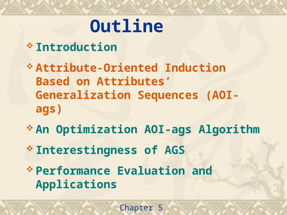
Outline Introduction
Attribute-Oriented Induction Based on Attributes’ Generalization Sequences (AOI-ags)
An Optimization AOI-ags Algorithm
Interestingness of AGS
Performance Evaluation and Applications
Chapter 5

Introduction
Chapter 5
Table 5.1. Some tuples of a plant distributed dataset
Tuple-ID Plant-name Veg-name Elevation /m Location t1 Orchid meadow [1000, 1500] Lijiang t2 Fig scrub [2400, 3000] Weixi t3 Magnolia scrub [3000, 3700] Lijiang t4 Calligonum taiga [2000, 3000] Jianchuan t5 Magnolia meadow [3000, 4000] Lanping t6 Agave taiga [3000, 4000] Lanping t7 Yucca forest [1500, 2400] Weixi t8 Waterlily meadow [800, 2200] Jianchuan
[800,3000](3,1)
[2000, 3000](3,1,2) [3000, 4000](3,2,2)
[1000, 1500](3,1,1,1) [800, 2400](3,1,1,2)
[800, 2200](3,1,1,2,1) [1500, 2400](3,1,1,2,2)
[2400, 3000](3,1,2,2)
[800, 2400](3,1,1) [3000, 3700](3,2,1)
[2000, 3000](3,1,2,1)
[800, 4000](3)
4
1
2
3
5
Level
[3000,4000](3,2)
Figure 5.1 An example of a concept hierarchy tree
(1). Attribute threshold control
(2). Relation threshold control
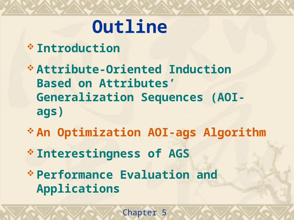
Outline Introduction
Attribute-Oriented Induction Based on Attributes’ Generalization Sequences (AOI-ags)
An Optimization AOI-ags Algorithm
Interestingness of AGS
Performance Evaluation and Applications
Chapter 5

Chapter 5
AOI-ags Method (1)
an attribute is generalized earlier or latter will not affect the final generalization result.
a generalization result is the same no matter that it is obtained by generalizing gradually or directly up to the k-th level

Chapter 5
Definition 5.2 Given a relation pattern ),,( 1 mAAR , attributes’ concept
hierarchy trees mhh ,,1 , the Heights of trees mll ,,1 , sequence mi gm
gi
g AAA 11 is
called an AGS of AOI, where ( 11 ii lg ).
Property 5.1 The number of all AGS in a relation pattern is
m
iil
1
)1(。
Proof. One sequence mi ggg 1 can only confirm one AGS mi g
mgi
g AAA 11 .
Meanwhile, 11 ii lg 1|| ii lg )1( mi
The number of attributes’ generalization sequences is:
m
iimi llll
11 )1()1()1()1( □
AOI-ags Method (2)

Chapter 5
Definition 5.3 Given the relation threshold control Z.
If the generalization relation ),( 1 nrrr which are
confirmed by the AGS mi g
mgi
g AAA 11 ( 11 ii lg )
satisfies Znn )/(1 , and if increasing any )1( mig i , it
will not satisfy Znn )/(1 , then mg
mg AA 1
1 is called an
AGS which satisfies the Z, and ),( 1 nrrr is called a
generalization result undermg
mg AA 1
1
AOI-ags Method (3)

Chapter 5
AOI-ags Method (4)
Algorithm 5.1 The ordinary AOI-ags algorithm
Description: 1) Gen_seq(relation,1,m,L1,S,Gs); 2) Selecting a sequence from the set Gs of AGS and returning a generalization relation; 3) Producing generalization rules from the generalization relation. Procedure Gen_seq(r,i,m,Li,S,Gs); // S is an AGS, Gs is a collection of AGSs which meet the Z (1) For k=Li+1 downto 1 Do (2) Begin If k<Li+1 then (3) Gen_r ← generalize(r,i,k) (4) Else Gen_r ← r
Endif; (5) If i<m then (6) Gen_seq (Gen_r,i+1,m,Li+1,S∪ Ak
i,Gs) (7) Else (8) If |Gen-r|≤ n(1-Z) then (9) Gs ← Gs∪ {S∪ Ak
i} endif Endif End
Outline Introduction
Attribute-Oriented Induction Based on Attributes’ Generalization Sequences (AOI-ags)
An Optimization AOI-ags Algorithm
Interestingness of AGS
Performance Evaluation and Applications
Chapter 5

Chapter 5
An Optimization AOI-ags Algorithm (1)
(1). AOI-ags and Partition :
Table 5.1. Some tuples of a plant distributed dataset
Tuple-ID Plant-name Veg-name Elevation /m Location t1 Orchid meadow [1000, 1500] Lijiang t2 Fig scrub [2400, 3000] Weixi t3 Magnolia scrub [3000, 3700] Lijiang t4 Calligonum taiga [2000, 3000] Jianchuan t5 Magnolia meadow [3000, 4000] Lanping t6 Agave taiga [3000, 4000] Lanping t7 Yucca forest [1500, 2400] Weixi t8 Waterlily meadow [800, 2200] Jianchuan
rrr ixix |
an equivalence partition of r under X
kx ,,1 , ky ,,1 , YX = yjxiji ,|
intersection partition YXYX

Chapter 5
An Optimization AOI-ags Algorithm (2)
},{ 1 mAAR is the relation r
there is a one-one correspondence from the records of r to equivalence classes
of }{}{ 1 mAA
)11,1(, ijA ljmii
the generalization relation and a equivalence class
mm gAgA 11
under AGSmg
mg AA 1
1 is corresponding one by one

Chapter 5
An Optimization AOI-ags Algorithm (3)
A new partition-based approach of AOI-ags:
(1) Compute all)11,1(, iigA lgmi
ii
.
(2) Obtain all AGS which meet the Z.
(3) Select a sequencemg
mg AA 1
1 , and then calculate generalization
relation mm gAgAr 11 .
(4) Produce generalization rules from the generalization relation.

Chapter 5
An Optimization AOI-ags Algorithm (4)
(2) Searching Space and Pruning Strategies
Definition 5.4 The Grid that is constituted by
m
iil
1
)1(possible AGS and satisfies the following properties is
called the searching space.
(1) There are AGS that satisfy 11 kgg m in the k-th level.
(2) Each sequence is connected to any sequence mi g
mgi
g AAA 11
1
of the (k-1)-th level.

Chapter 5
An Optimization AOI-ags Algorithm (5)
Example 5.2 Given two attributes A1 and A2, the Heights of the concept hierarchy trees are l1=2, l2=3, then the searching space is showed as figure 5.2
12
11 AA
22
11 AA
32
11 AA
22
21 AA
12
31 AA
32
21 AA
42
11 AA
32
31 AA
22
31 AA
42
21 AA
42
31 AA
12
21 AA
1
2
3
4
5
6
Figure 5.2 An example of the searching space
Level
Chapter 5
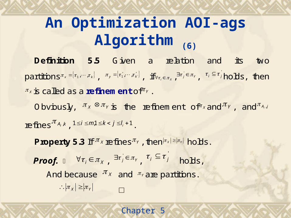
An Optimization AOI-ags Algorithm (6)
Definition 5.5 Given a relation and its two
partitions kx ,,1 , ky ,,1 , if Xi , Yj '
, 'ji holds, then
X is called as a refinement of Y .
Obviously, YX is the refinement of X and Y , and jAi ,
refines kAi , , 11,1 iljkmi .
Property 5.3 If X refines Y , then YX holds.
Proof. Xi , Yj '
, 'ji holds,
And because X and Y are partitions.
YX □
Chapter 5
An Optimization AOI-ags Algorithm (7)
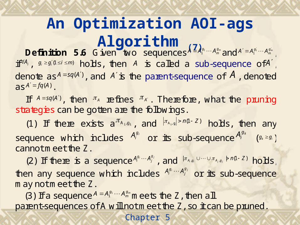
Definition 5.6 Given two sequences mgm
g AAA 11 and mg
mg AAA 1
1 , if iA , )1( migg ii holds, then A is called a sub-sequence of A, denote as )(AsqA , and Ais the parent-sequence of A , denoted as )(AfqA .
If )(AsqA , then A refines A . Therefore, what the pruning strategies can be gotten are the followings.
(1) If there exists a ii g,A , and )1(ii ,gA Zn holds, then any
sequence which includes ig
iA or its sub-sequencekg
iA ( ik gg ) cannot meet the Z.
(2) If there is a sequenceji
gj
gi AA , and )1(|| ,, Zn
jjii gAgA holds,
then any sequence which includes ji
gj
gi AA or its sub-sequence
may not meet the Z. (3) If a sequence
mgm
g AAA 11 meets the Z, then all
parent-sequences of A will not meet the Z, so it can be pruned.

Chapter 5
(3) Equivalence Partition Trees and Calculating (1)ii g,A
Definition 5.7 The equivalence partition tree of the attribute A
Table 5.1. Some tuples of a plant distributed dataset
Tuple-ID Plant-name Veg-name Elevation /m Location t1 Orchid meadow [1000, 1500] Lijiang t2 Fig scrub [2400, 3000] Weixi t3 Magnolia scrub [3000, 3700] Lijiang t4 Calligonum taiga [2000, 3000] Jianchuan t5 Magnolia meadow [3000, 4000] Lanping t6 Agave taiga [3000, 4000] Lanping t7 Yucca forest [1500, 2400] Weixi t8 Waterlily meadow [800, 2200] Jianchuan
[800,3000](3,1)
[2000, 3000](3,1,2) [3000, 4000](3,2,2)
[1000, 1500](3,1,1,1) [800, 2400](3,1,1,2)
[800, 2200](3,1,1,2,1) [1500, 2400](3,1,1,2,2)
[2400, 3000](3,1,2,2)
[800, 2400](3,1,1) [3000, 3700](3,2,1)
[2000, 3000](3,1,2,1)
[800, 4000](3)
4
1
2
3
5
Level
[3000,4000](3,2)
Figure 5.1 An example of a concept hierarchy tree
null
Partition level
2
0
1
2
3
4
5
1 2
3
1
2
1
2
1
1
1
{t7}
{t1}
{t8}
{t2}
{t5,t6} {t3} 2
{t4} 2
Chapter 5
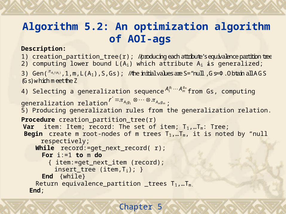
Algorithm 5.2: An optimization algorithm of AOI-ags
Description: 1) creation_partition_tree(r); //producing each attribute’s equivalence partition tree 2) computing lower bound L(Ai) which attribute Ai is generalized;
3) Gen( )( 1,1 AlA ,1,m,L(A1),S,Gs); //the initial values are S=“null”, Gs=Φ. Obtain all AGS (Gs) which meet the Z
4) Selecting a generalization sequencemg
mg AA 1
1 from Gs, computing
generalization relation mm gAgAr 11 ;
5) Producing generalization rules from the generalization relation.
Procedure creation_partition_tree(r) Var item: Item; record: The set of item; T1,…Tm: Tree; Begin create m root-nodes of m trees T1,…Tm, it is noted by “null”
respectively; While record:=get_next_record( r); For i:=1 to m do { item:=get_next_item (record); insert_tree (item,Ti); } End {while} Return equivalence_partition _trees T1,…Tm. End;

Chapter 5
Algorithm 5.2: An optimization algorithm of AOI-ags
Procedure Gen(r,i,m,L(Ai),S,Gs); (1) For k= L(Ai) downto 1 Do (2) Begin If i=1 and k < L(A1) then
(3) Gen_r ← kAi , (4) Else If i=1 and k= L(A1) then (5) Gen_r ← r
(6) Else Gen_r ← kAir , Endif
Endif; (7) if | Gen_r| > n(1-Z) then (8) exit for
endif (9) If i<m then (10) Gen (Gen_r,i+1,m,L(Ai+1),S∪ Aki,Gs) (11) Else If |Gen-r|≤ n(1-Z) then (12) Gs ← Gs∪ {S∪ Aki}; (13) Exit for Endif Endif End

Outline Introduction
Attribute-Oriented Induction Based on Attributes’ Generalization Sequences (AOI-ags)
An Optimization AOI-ags Algorithm
Interestingness of AGS
Performance Evaluation and Applications
Chapter 5

Chapter 5
Interestingness of AGS (1) Motivation example: For the plant “Magnolia sieboldii” in a plant
distributed dataset, suppose the following rules have been obtained.
(1) Plant “Magnolia sieboldii” ⇒ 50% grows in the conifer forest
and scrub whose elevation is from 2600 to 4100 meter of Lijiang,
and 50% grows in the forest, scrub and meadow whose
elevation is from 2400 to 3900 meter of Weixi.
(2) Plant “Magnolia sieboldii” ⇒ 90% grows in the conifer forest
and scrub whose elevation is from 2600 to 4100 meter of Lijiang,
and 10% grows in the forest, scrub and meadow whose
elevation is from 2400 to 3900 meter of Weixi.
The rule (2) is more meaningful than the rule (1), because the
growth characteristics of plant “Magnolia sieboldii” are more
obvious in the rule (2).
Chapter 5
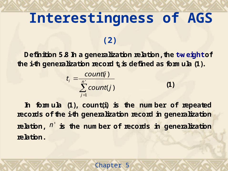
Interestingness of AGS (2)
Definition 5.8 In a generalization relation, the t-weight of the i-th generalization record ti is defined as formula (1).
'
1
)(
)(n
j
i
jcount
icountt
(1)
In formula (1), count(i) is the number of repeated records of the i-th generalization record in generalization
relation, 'n is the number of records in generalization
relation.
Chapter 5
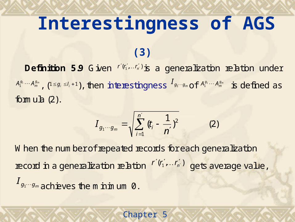
Interestingness of AGS (3)
Definition 5.9 Given ),( 1 nrrr is a generalization relation under mg
mg AA 1
1 , ( 11 ii lg ), then interestingness mggI 1 of mgm
g AA 11 is defined as
formula (2).
n
iigg n
tIm
1
2)1
(1
(2)
When the number of repeated records for each generalization
record in a generalization relation ),( 1 nrrr gets average value,
mggI 1 achieves the minimum 0.
Outline Introduction
Attribute-Oriented Induction Based on Attributes’ Generalization Sequences (AOI-ags)
An Optimization AOI-ags Algorithm
Interestingness of AGS
Performance Evaluation and Applications
Chapter 5

Chapter 5
Performance Evaluation and Applications (1)
(a) (b)
z=0. 8, m=2
0
500
1000
1500
100 300 500 1000 3000
The n val ue
Runt
ime
(s)
A. 2
A. 1
n=200, z=0. 8
0
1000
2000
3000
4000
2 3 5 7 8 10
The m val ue
Runtime (s)
A. 2
A. 1
Figure 5.4 Performance of algorithms using synthetic datasets

Chapter 5
Performance Evaluation and Applications (2)
Figure 5.5 Characters of fast re-generalization for the two algorithms
(a) (b)
n=500, m=3
0
200
400
600
800
0. 4 0. 5 0. 6 0. 7 0. 8 0. 9
the Z val ue
Runtime(s)
A. 1
n=1000, m=5
05
1015
2025
0. 4 0. 5 0. 6 0. 7 0. 8 0. 9
the z val ue
Runt
ime(
s)
A. 2

Chapter 5
Applications in a Real Dataset The followings are some examples:--“Tricholoma matsutake” 40% grows in the fore⇒
st and meadow whose elevation is from 3300 to 4100 meter of Lijiang.
--“Angiospermae” 80% grows in the forest⇒ 、 scrub and meadow whose elevation is from 2400 to 3900 meter of Lijiang and Weixi.
--Lijiang There are a plenty of plants species in s⇒evere danger such as “Tricholoma matsutake”, “Angiospermae”, “Gymnospermae”.

Conclusions
In this chapter, first, by introducing a new concept of attributes’ generalization sequences, AOI-ags method was proposed.
Second, an optimization AOI-ags algorithm was discussed.
Third, by defining the interestingness of AGS, the selection problem of AGS is solved.
Fourth, Performance Evaluation and Applications
Chapter 5
Thanks!
Any questions?