apex user manual - research

APEXTM User Manual

EDAX Inc.Ametek Materials Analysis Division

Contents

1 Introduction to APEX™ 11.1 Launching APEX™ . . . . . . . . . . . . . . . . . . . . . . . . . . . . . . . . . . . . . 11.2 Layout Overview . . . . . . . . . . . . . . . . . . . . . . . . . . . . . . . . . . . . . . 21.3 Icons . . . . . . . . . . . . . . . . . . . . . . . . . . . . . . . . . . . . . . . . . . . . . 41.4 User Profile Preferences . . . . . . . . . . . . . . . . . . . . . . . . . . . . . . . . . . 71.5 Project Tree Panel . . . . . . . . . . . . . . . . . . . . . . . . . . . . . . . . . . . . . . 111.6 Collection Modes . . . . . . . . . . . . . . . . . . . . . . . . . . . . . . . . . . . . . . 141.7 Multi-user Mode . . . . . . . . . . . . . . . . . . . . . . . . . . . . . . . . . . . . . . 151.8 Administrator Feature . . . . . . . . . . . . . . . . . . . . . . . . . . . . . . . . . . . . 17

2 Image and Data Collection 212.1 Image Collection . . . . . . . . . . . . . . . . . . . . . . . . . . . . . . . . . . . . . . 212.2 Spectrum Collection and Settings . . . . . . . . . . . . . . . . . . . . . . . . . . . . . . 222.3 Linescan Collection and Settings . . . . . . . . . . . . . . . . . . . . . . . . . . . . . . 242.4 X-Ray Map Collection and Settings . . . . . . . . . . . . . . . . . . . . . . . . . . . . 26

2.4.1 ROI display, custom ROI and changing elements while mapping: . . . . . . . . . 302.4.2 NET and ROI Map Options: . . . . . . . . . . . . . . . . . . . . . . . . . . . . 302.4.3 Smart Phase Mapping . . . . . . . . . . . . . . . . . . . . . . . . . . . . . . . 31

2.5 Drift Correction . . . . . . . . . . . . . . . . . . . . . . . . . . . . . . . . . . . . . . . 322.5.1 Drift Correction View Window . . . . . . . . . . . . . . . . . . . . . . . . . . . 32

2.6 Mulitifield Scan Table . . . . . . . . . . . . . . . . . . . . . . . . . . . . . . . . . . . . 34

3 Data Analysis and Display 353.1 Import, Export, and Merge Data . . . . . . . . . . . . . . . . . . . . . . . . . . . . . . 353.2 Quant View Window . . . . . . . . . . . . . . . . . . . . . . . . . . . . . . . . . . . . 373.3 Spectrum View Window . . . . . . . . . . . . . . . . . . . . . . . . . . . . . . . . . . 41

3.3.1 Spectrum View Toolbars . . . . . . . . . . . . . . . . . . . . . . . . . . . . . . 433.3.2 Spectrum View Advanced Settings . . . . . . . . . . . . . . . . . . . . . . . . . 473.3.3 Additional Spectra Overlay Methods: . . . . . . . . . . . . . . . . . . . . . . . 493.3.4 Spectrum View Color Settings: . . . . . . . . . . . . . . . . . . . . . . . . . . . 493.3.5 Multi-spectra View . . . . . . . . . . . . . . . . . . . . . . . . . . . . . . . . . 513.3.6 Spectrum Matching (Optional): . . . . . . . . . . . . . . . . . . . . . . . . . . 52

3.4 Linescan View→ Image Window . . . . . . . . . . . . . . . . . . . . . . . . . . . . . 563.5 Multi-Map View Window . . . . . . . . . . . . . . . . . . . . . . . . . . . . . . . . . . 563.6 Mapping Pop-Up Menu: . . . . . . . . . . . . . . . . . . . . . . . . . . . . . . . . . . 60

4 Review Mode and Toolbars 63

4.1 Spectrum Review . . . . . . . . . . . . . . . . . . . . . . . . . . . . . . . . . . . . . . 634.2 Linescan Review . . . . . . . . . . . . . . . . . . . . . . . . . . . . . . . . . . . . . . 654.3 Mapping Review . . . . . . . . . . . . . . . . . . . . . . . . . . . . . . . . . . . . . . 66

5 Reporting and Printing 695.1 Report Generation: Live Mode . . . . . . . . . . . . . . . . . . . . . . . . . . . . . . . 695.2 Spectrum or Linescan Report: Review Mode . . . . . . . . . . . . . . . . . . . . . . . . 725.3 X-Ray Map Report: Review Mode . . . . . . . . . . . . . . . . . . . . . . . . . . . . . 745.4 Print Results . . . . . . . . . . . . . . . . . . . . . . . . . . . . . . . . . . . . . . . . . 74

6 Data Handling and Backup 776.1 Export and Backup Data . . . . . . . . . . . . . . . . . . . . . . . . . . . . . . . . . . 776.2 Automated Data and Database Backup . . . . . . . . . . . . . . . . . . . . . . . . . . . 796.3 Manual Data Backup . . . . . . . . . . . . . . . . . . . . . . . . . . . . . . . . . . . . 806.4 Restore the APEX™Database . . . . . . . . . . . . . . . . . . . . . . . . . . . . . . . 80

7 Advanced Settings 817.1 Detector Cooling and Slide Control . . . . . . . . . . . . . . . . . . . . . . . . . . . . 817.2 Microscope Column and Stage Control . . . . . . . . . . . . . . . . . . . . . . . . . . . 837.3 Spectral Calibration . . . . . . . . . . . . . . . . . . . . . . . . . . . . . . . . . . . . . 837.4 APEX™Tutorials Panel . . . . . . . . . . . . . . . . . . . . . . . . . . . . . . . . . . . 86

Chapter 1

Introduction to APEX™

1.1 Launching APEX™

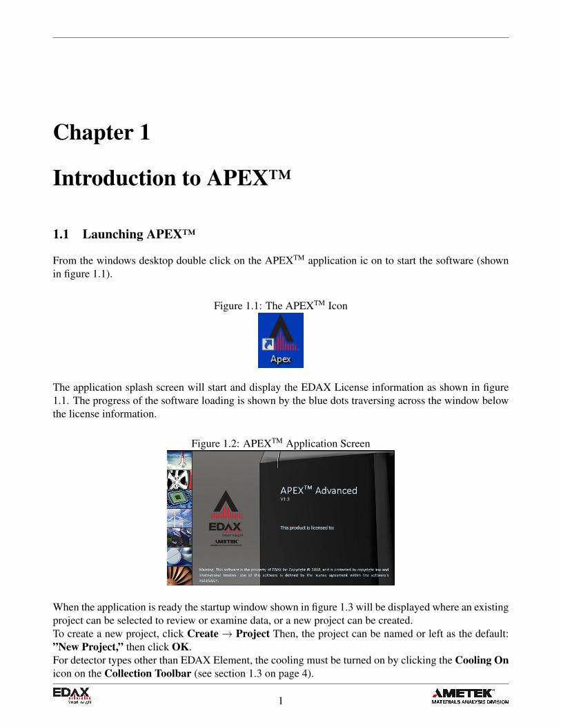
From the windows desktop double click on the APEXTM application ic on to start the software (shownin figure 1.1).

Figure 1.1: The APEXTM Icon

The application splash screen will start and display the EDAX License information as shown in figure1.1. The progress of the software loading is shown by the blue dots traversing across the window belowthe license information.

Figure 1.2: APEXTM Application Screen

When the application is ready the startup window shown in figure 1.3 will be displayed where an existingproject can be selected to review or examine data, or a new project can be created.To create a new project, click Create→ Project Then, the project can be named or left as the default:”New Project,” then click OK.For detector types other than EDAX Element, the cooling must be turned on by clicking the Cooling Onicon on the Collection Toolbar (see section 1.3 on page 4).

1

1.2. LAYOUT OVERVIEW

Figure 1.3: APEXTM Launch Screen (Live Collection Window)

1.2 Layout Overview

The title of the window displays which mode APEXTM is in. It has two states: a live collection windowand a review window. EDAX APEXTMis the data collection window, while EDAX APEXTM Review iswhere you can review all types of data and produce reports.

Figure 1.4: APEXTM Review Layout

• One of the many powerful features of the APEXTM is the two windows in which you can collectand review data simultaneously.

2

1.2. LAYOUT OVERVIEW

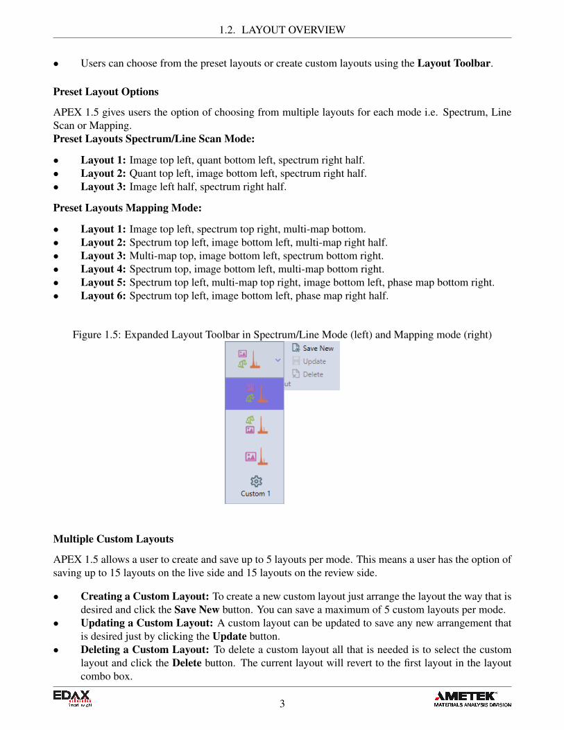
• Users can choose from the preset layouts or create custom layouts using the Layout Toolbar.

Preset Layout Options

APEX 1.5 gives users the option of choosing from multiple layouts for each mode i.e. Spectrum, LineScan or Mapping.Preset Layouts Spectrum/Line Scan Mode:

• Layout 1: Image top left, quant bottom left, spectrum right half.• Layout 2: Quant top left, image bottom left, spectrum right half.• Layout 3: Image left half, spectrum right half.

Preset Layouts Mapping Mode:

• Layout 1: Image top left, spectrum top right, multi-map bottom.• Layout 2: Spectrum top left, image bottom left, multi-map right half.• Layout 3: Multi-map top, image bottom left, spectrum bottom right.• Layout 4: Spectrum top, image bottom left, multi-map bottom right.• Layout 5: Spectrum top left, multi-map top right, image bottom left, phase map bottom right.• Layout 6: Spectrum top left, image bottom left, phase map right half.

Figure 1.5: Expanded Layout Toolbar in Spectrum/Line Mode (left) and Mapping mode (right)

Multiple Custom Layouts

APEX 1.5 allows a user to create and save up to 5 layouts per mode. This means a user has the option ofsaving up to 15 layouts on the live side and 15 layouts on the review side.

• Creating a Custom Layout: To create a new custom layout just arrange the layout the way that isdesired and click the Save New button. You can save a maximum of 5 custom layouts per mode.

• Updating a Custom Layout: A custom layout can be updated to save any new arrangement thatis desired just by clicking the Update button.

• Deleting a Custom Layout: To delete a custom layout all that is needed is to select the customlayout and click the Delete button. The current layout will revert to the first layout in the layoutcombo box.

3

1.3. ICONS

Figure 1.6 shows a new custom layout selected in APEX Reviews Spectrum mode. Once the layout issaved it will be selected and a new Custom Layout Icon appears in layout the combo box. The Updateand Delete buttons become active when a custom layout is selected. You can see a thumbnail tooltip ofa custom layout by hovering over it with the mouse (See Figure ??).

Figure 1.6: Custom Layout

Figure 1.7: Custom Layout with a Thumbnail Preview

To fine tune the layout of windows, move the mouse pointer over the splitter sections (see red circle infigure 1.8) between windows to change the size of each of the windows. The individual windows can alsobe detached from the general user interface by clicking and dragging in the header bar of the window.The detached windows can re-arranged independently of other windows, moved to secondary monitors,or be re-docked by moving to an edge in the user interface or hovering over one of the dock icons thatshow up when moving the window.

Figure 1.8: Layout Options

1.3 Icons

Title Bar Toolbar

The title bar toolbar shown in figure 1.9 allows the user to show or hide different view panels in order toeasily view spectra, quant, and mapping results. As APEXTM can display live quant results while data iscollecting, these icons are especially useful.

Figure 1.9: The Title Bar Toolbar

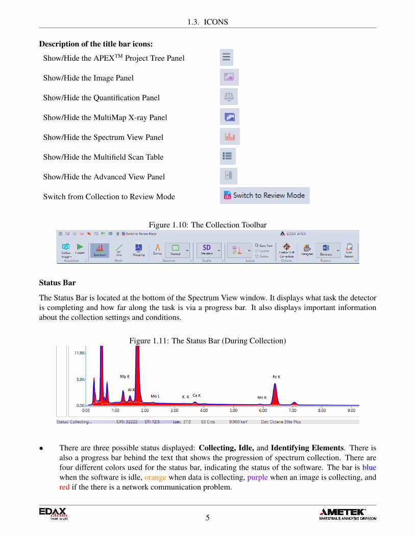
Collection Toolbar

Below the title bar toolbar is the collection toolbar (figure 1.10) which enables users to set up datacollection easily: moving from left to right across the top of the page. The icon next to the ImageCollection icon will be Detector Cooling if detector is not ready, and be replaced by the Data CollectionStart/Stop icon once detector is ready.

4

1.3. ICONS

Description of the title bar icons:

Show/Hide the APEXTM Project Tree Panel

Show/Hide the Image Panel

Show/Hide the Quantification Panel

Show/Hide the MultiMap X-ray Panel

Show/Hide the Spectrum View Panel

Show/Hide the Multifield Scan Table

Show/Hide the Advanced View Panel

Switch from Collection to Review Mode

Figure 1.10: The Collection Toolbar

Status Bar

The Status Bar is located at the bottom of the Spectrum View window. It displays what task the detectoris completing and how far along the task is via a progress bar. It also displays important informationabout the collection settings and conditions.

Figure 1.11: The Status Bar (During Collection)

• There are three possible status displayed: Collecting, Idle, and Identifying Elements. There isalso a progress bar behind the text that shows the progression of spectrum collection. There arefour different colors used for the status bar, indicating the status of the software. The bar is bluewhen the software is idle, orange when data is collecting, purple when an image is collecting, andred if the there is a network communication problem.

5

1.3. ICONS

Description of the collection icons:

The Image Collection Icon

The Detector Cooling Icon

The Data Collection Start/ Stop Icon

The Collection Mode Icons

The Spectrum Mode Icons

The Collection Quality Icon

The Drift Correction Icon

The Report Generation Icons

The Auto Report Icon

6

1.4. USER PROFILE PREFERENCES

Collection Conditions:

The display of the status bar can be customized in User Preferences (see section 1.4).

• CPS : The EDS Detector total counts per second.• DT : The Dead Time percentage (updated once per second).• Lsec: The live time (in seconds) for the current spectrum.• Cnts: The intensity (in counts) at the energy cursor position.• keV: The energy (in keV) at the energy cursor position.• Det: The model type of the EDS Detector.

1.4 User Profile Preferences

The user profile preferences allows users to customize the display and storage options to best meet theirneeds. To access the user profile menu, click the User Profile Icon in the top right on the screen. Thiswill pull up the User Preferences tab, pictured below. The display and storage options are describedbelow. The User Account tab enables a user First Name and Last Name to be entered for the account(see Figure 1.14). This name will be used for reports. The User Name is automatically set to ApexData.For more information on data backup and handling settings, see section 6.1 on page 77.

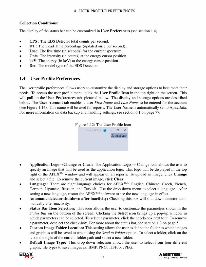
Figure 1.12: The User Profile Icon

• Application Logo→Change or Clear: The Application Logo→ Change icon allows the user tospecify an image that will be used as the application logo. This logo will be displayed in the topright of the APEXTM window and will appear on all reports. To upload an image, click Changeand select a file. To remove the current image, click Clear.

• Language: There are eight language choices for APEXTM: English, Chinese, Czech, French,German, Japanese, Russian, and Turkish. Use the drop down menu to select a language. Aftersetting a new language, restart the APEXTM software to see the new language in effect.

• Automatic detector shutdown after inactivity: Checking this box will shut down detector auto-matically after inactivity.

• Status Bar Item Selection: This icon allows the user to customize the parameters shown in theStatus Bar on the bottom of the screen. Clicking the Select icon brings up a pop-up window inwhich parameters can be selected. To select a parameter, click the check-box next to it. To removea parameter, deselect the check-box. For more about the status bar, see section 1.3 on page 5.

• Custom Image Folder Location: This setting allows the user to define the folder to which imagesand graphics will be saved to when using the Send to Folder option. To select a folder, click on the. . . on the right of the current folder path and select a new folder.

• Default Image Type: This drop-down selection allows the user to select from four differentgraphic file types to save images as: BMP, PNG, TIFF, or JPEG.

7


Figure 1.13: The User Profile Selection Window

Figure 1.14: Change User Account Window

Figure 1.15: Language Drop Down Menu

8


Figure 1.16: Status Bar Items

Figure 1.17: Image Folder and Image Type Selection

Figure 1.18: Storage Drive Selection

9


• Storage Drive: This selection is to define where the APEX raw data (Spectrum, Linescan, andMaps) are saved. Typically, this is the C drive but other internal hard drive locations can be used.

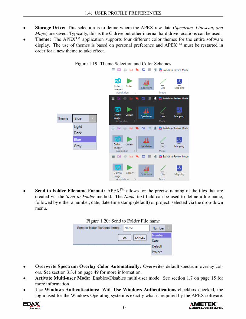
• Theme: The APEXTM application supports four different color themes for the entire softwaredisplay. The use of themes is based on personal preference and APEXTM must be restarted inorder for a new theme to take effect.

Figure 1.19: Theme Selection and Color Schemes

• Send to Folder Filename Format: APEXTM allows for the precise naming of the files that arecreated via the Send to Folder method. The Name text field can be used to define a file name,followed by either a number, date, date-time stamp (default) or project, selected via the drop-downmenu.

Figure 1.20: Send to Folder File name

• Overwrite Spectrum Overlay Color Automatically: Overwrites default spectrum overlay col-ors. See section 3.3.4 on page 49 for more information.

• Activate Multi-user Mode: Enables/Disables multi-user mode. See section 1.7 on page 15 formore information.

• Use Windows Authentications: With Use Windows Authentications checkbox checked, thelogin used for the Windows Operating system is exactly what is required by the APEX software.

10

1.5. PROJECT TREE PANEL

See Section 1.8 on page 18 for more information.• Report Paper Size: Chooses between Letter and A4 for the report paper size.

1.5 Project Tree Panel

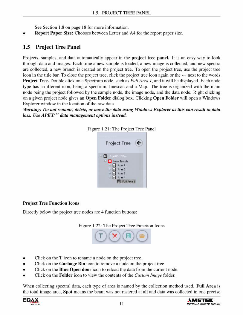
Projects, samples, and data automatically appear in the project tree panel. It is an easy way to lookthrough data and images. Each time a new sample is loaded, a new image is collected, and new spectraare collected, a new branch is created on the project tree. To open the project tree, use the project treeicon in the title bar. To close the project tree, click the project tree icon again or the← next to the wordsProject Tree. Double click on a Spectrum node, such as Full Area 1, and it will be displayed. Each nodetype has a different icon, being a spectrum, linescan and a Map. The tree is organized with the mainnode being the project followed by the sample node, the image node, and the data node. Right clickingon a given project node gives an Open Folder dialog box. Clicking Open Folder will open a WindowsExplorer window in the location of the raw data.Warning: Do not rename, delete, or move the data using Windows Explorer as this can result in dataloss. Use APEXTM data management options instead.

Figure 1.21: The Project Tree Panel

Project Tree Function Icons

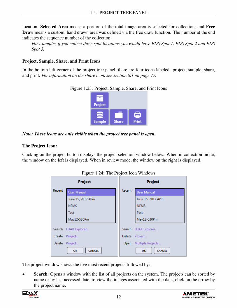
Directly below the project tree nodes are 4 function buttons:

Figure 1.22: The Project Tree Function Icons

• Click on the T icon to rename a node on the project tree.• Click on the Garbage Bin icon to remove a node on the project tree.• Click on the Blue Open door icon to reload the data from the current node.• Click on the Folder icon to view the contents of the Custom Image folder.

When collecting spectral data, each type of area is named by the collection method used. Full Area isthe total image area, Spot means the beam was not rastered at all and data was collected in one precise

11


location, Selected Area means a portion of the total image area is selected for collection, and FreeDraw means a custom, hand drawn area was defined via the free draw function. The number at the endindicates the sequence number of the collection.

For example: if you collect three spot locations you would have EDS Spot 1, EDS Spot 2 and EDSSpot 3.

Project, Sample, Share, and Print Icons

In the bottom left corner of the project tree panel, there are four icons labeled: project, sample, share,and print. For information on the share icon, see section 6.1 on page 77.

Figure 1.23: Project, Sample, Share, and Print Icons

Note: These icons are only visible when the project tree panel is open.

The Project Icon:

Clicking on the project button displays the project selection window below. When in collection mode,the window on the left is displayed. When in review mode, the window on the right is displayed.

Figure 1.24: The Project Icon Windows

The project window shows the five most recent projects followed by:

• Search: Opens a window with the list of all projects on the system. The projects can be sorted byname or by last accessed date, to view the images associated with the data, click on the arrow bythe project name.

12


• Create: Creates a new project.• Delete: Opens a window where a saved project can be deleted. To review the selected project,

click on the Open button. The images from the projects are displayed to remind the user of thecontents of the project.

• Open: Multiple Projects: When in review mode multiple projects can be opened and loaded tothe project tree.

Figure 1.25: The EDAX Explorer and Multiple Project Windows

The Sample Icon:

The sample icon displays the sample selection window. To open an existing sample, double click onthe sample in the list. To create a new sample, click on the New text-box and enter a name for the newsample.

Figure 1.26: The Sample Window

13

1.6. COLLECTION MODES

The Print Icon:

The print icon outputs a screen capture of the entire APEXTM window to the printer. To print specificportions of the screen (i.e. the image, spectrum, or quant results) save the item to the custom folder andthen open to print.

1.6 Collection Modes

There are three main modes for collection in APEXTM: spectrum, linescan, and X-ray map. These modesare used to achieve different types of data sets, depending on the nature of the user’s work.

Figure 1.27: The Collection Mode Icons

Spectrum

The spectrum mode collects a spectrum of the selected area for a period of time, set by the user. Thereare two options for spectrum collection: Survey and Normal.

Figure 1.28: The Spectrum Mode Icons and Drop-down Menu

• When in Survey Mode a spectrum collection will start as soon as a point or area is selected inthe SEM image. Selection a new point or area will restart the acquisition making it easy to clickaround in the image and identify features of interest. It is a good, quick way to get an overview ofwhat materials are in a specimen, but the spectrum will not be saved after collection.

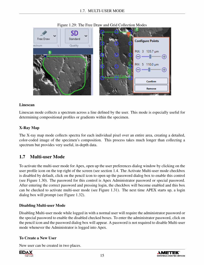
• The Normal Mode has three different settings: normal, free draw, and grid:

• Normal: Allows the user to define analysis locations individually.• Free Draw: The free draw mode allows to the user to draw any shape onto the image area

area for analysis.• Grid: Allows the user to define a matrix of equidistant points for which the spectra will be

collected sequentially.

14

1.7. MULTI-USER MODE

Figure 1.29: The Free Draw and Grid Collection Modes

Linescan

Linescan mode collects a spectrum across a line defined by the user. This mode is especially useful fordetermining compositional profiles or gradients within the specimen.

X-Ray Map

The X-ray map mode collects spectra for each individual pixel over an entire area, creating a detailed,color-coded image of the specimen’s composition. This process takes much longer than collecting aspectrum but provides very useful, in-depth data.

1.7 Multi-user Mode

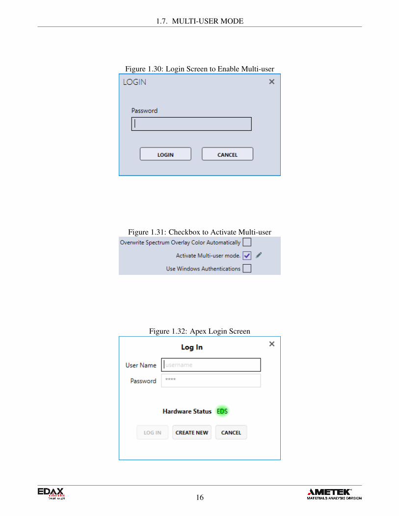
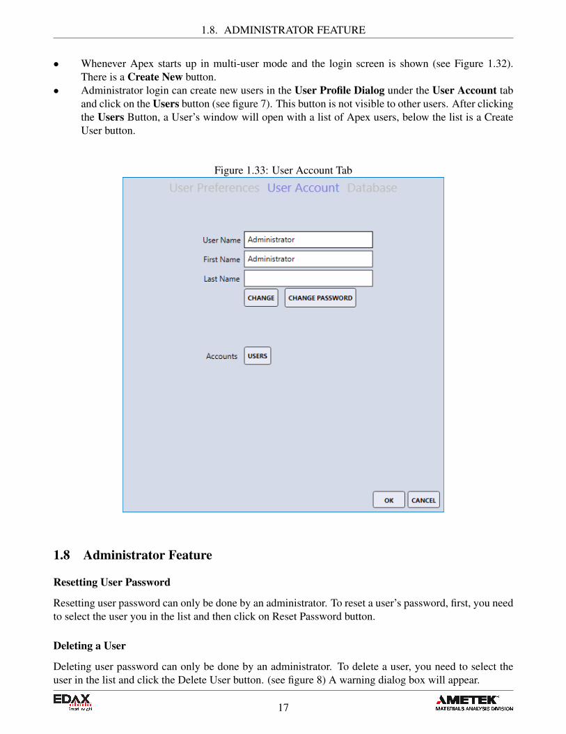
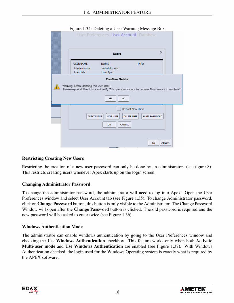
To activate the multi-user mode for Apex, open up the user preferences dialog window by clicking on theuser profile icon on the top right of the screen (see section 1.4. The Activate Multi-user mode checkboxis disabled by default, click on the pencil icon to open up the password dialog box to enable this control(see Figure 1.30). The password for this control is Apex Administrator password or special password.After entering the correct password and pressing login, the checkbox will become enabled and this boxcan be checked to activate multi-user mode (see Figure 1.31). The next time APEX starts up, a logindialog box will prompt (see Figure 1.32).

Disabling Multi-user Mode

Disabling Multi-user mode while logged in with a normal user will require the administrator password orthe special password to enable the disabled checked boxes. To enter the administrator password, click onthe pencil icon and the password dialog box will appear. A password is not required to disable Multi-usermode whenever the Administrator is logged into Apex.

To Create a New User

New user can be created in two places.

15

1.7. MULTI-USER MODE

Figure 1.30: Login Screen to Enable Multi-user

Figure 1.31: Checkbox to Activate Multi-user

Figure 1.32: Apex Login Screen

16

1.8. ADMINISTRATOR FEATURE

• Whenever Apex starts up in multi-user mode and the login screen is shown (see Figure 1.32).There is a Create New button.

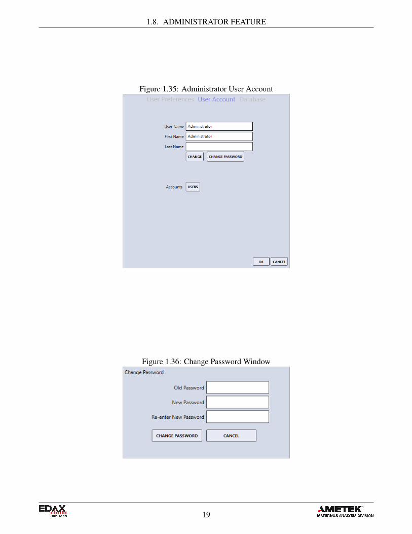
• Administrator login can create new users in the User Profile Dialog under the User Account taband click on the Users button (see figure 7). This button is not visible to other users. After clickingthe Users Button, a User’s window will open with a list of Apex users, below the list is a CreateUser button.

Figure 1.33: User Account Tab

1.8 Administrator Feature

Resetting User Password

Resetting user password can only be done by an administrator. To reset a user’s password, first, you needto select the user you in the list and then click on Reset Password button.

Deleting a User

Deleting user password can only be done by an administrator. To delete a user, you need to select theuser in the list and click the Delete User button. (see figure 8) A warning dialog box will appear.

17


Figure 1.34: Deleting a User Warning Message Box

Restricting Creating New Users

Restricting the creation of a new user password can only be done by an administrator. (see figure 8).This restricts creating users whenever Apex starts up on the login screen.

Changing Administrator Password

To change the administrator password, the administrator will need to log into Apex. Open the UserPreferences window and select User Account tab (see Figure 1.35). To change Administrator password,click on Change Password button, this button is only visible to the Administrator. The Change PasswordWindow will open after the Change Password button is clicked. The old password is required and thenew password will be asked to enter twice (see Figure 1.36).

Windows Authentication Mode

The administrator can enable windows authentication by going to the User Preferences window andchecking the Use Windows Authentication checkbox. This feature works only when both ActivateMulti-user mode and Use Windows Authentication are enabled (see Figure 1.37). With WindowsAuthentication checked, the login used for the Windows Operating system is exactly what is required bythe APEX software.

18


Figure 1.35: Administrator User Account

Figure 1.36: Change Password Window

19


Figure 1.37: Windows Authentication Mode Enabled

20

Chapter 2

Image and Data Collection

In order to collect a spectrum, line scan, or map, an image must be collected first. There are manydifferent settings to optimize image and data collection, depending on the nature of the work as well asthe process used. The settings for image and data collection are outlined below.

2.1 Image Collection

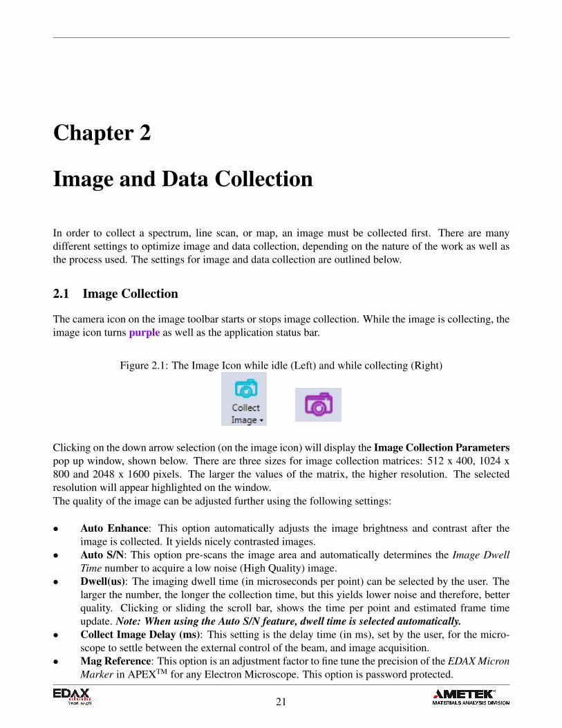
The camera icon on the image toolbar starts or stops image collection. While the image is collecting, theimage icon turns purple as well as the application status bar.

Figure 2.1: The Image Icon while idle (Left) and while collecting (Right)

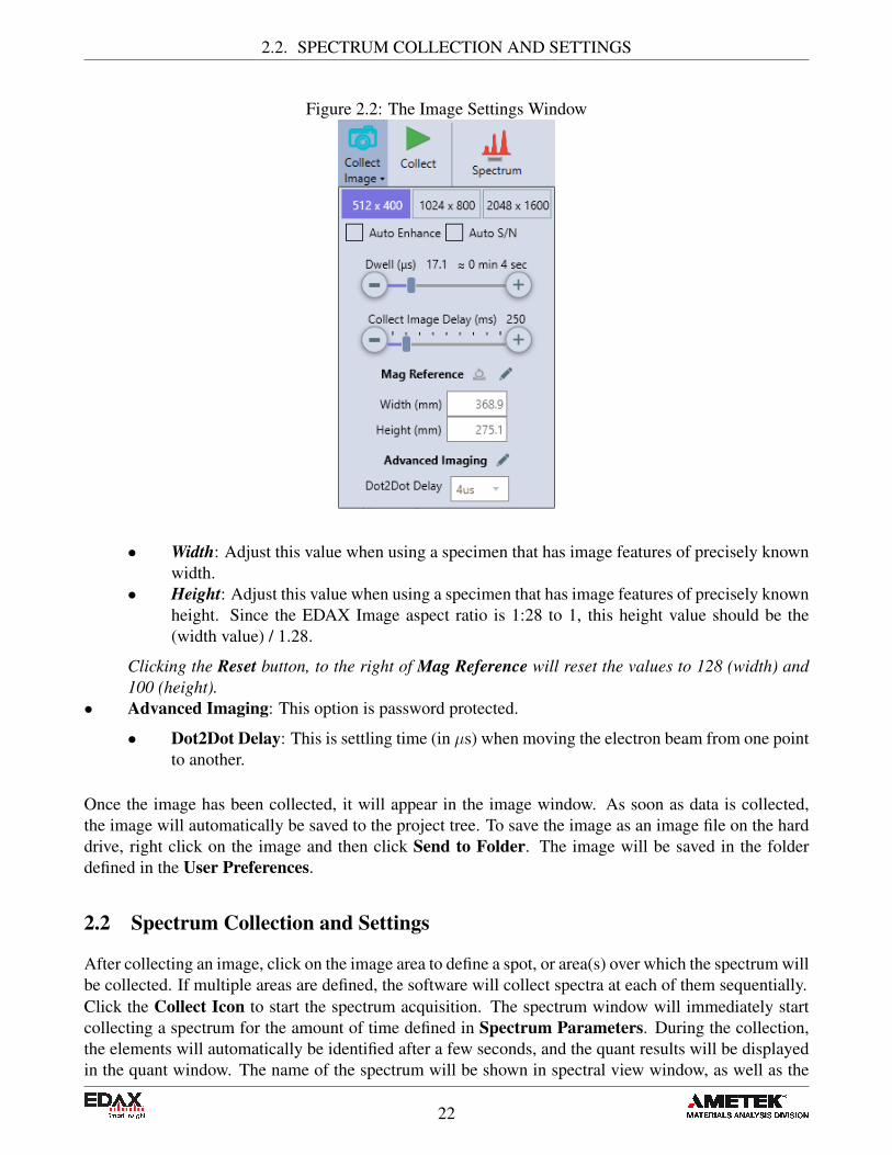
Clicking on the down arrow selection (on the image icon) will display the Image Collection Parameterspop up window, shown below. There are three sizes for image collection matrices: 512 x 400, 1024 x800 and 2048 x 1600 pixels. The larger the values of the matrix, the higher resolution. The selectedresolution will appear highlighted on the window.The quality of the image can be adjusted further using the following settings:

• Auto Enhance: This option automatically adjusts the image brightness and contrast after theimage is collected. It yields nicely contrasted images.

• Auto S/N: This option pre-scans the image area and automatically determines the Image DwellTime number to acquire a low noise (High Quality) image.

• Dwell(us): The imaging dwell time (in microseconds per point) can be selected by the user. Thelarger the number, the longer the collection time, but this yields lower noise and therefore, betterquality. Clicking or sliding the scroll bar, shows the time per point and estimated frame timeupdate. Note: When using the Auto S/N feature, dwell time is selected automatically.

• Collect Image Delay (ms): This setting is the delay time (in ms), set by the user, for the micro-scope to settle between the external control of the beam, and image acquisition.

• Mag Reference: This option is an adjustment factor to fine tune the precision of the EDAX MicronMarker in APEXTM for any Electron Microscope. This option is password protected.

21

2.2. SPECTRUM COLLECTION AND SETTINGS

Figure 2.2: The Image Settings Window

• Width: Adjust this value when using a specimen that has image features of precisely knownwidth.

• Height: Adjust this value when using a specimen that has image features of precisely knownheight. Since the EDAX Image aspect ratio is 1:28 to 1, this height value should be the(width value) / 1.28.

Clicking the Reset button, to the right of Mag Reference will reset the values to 128 (width) and100 (height).

• Advanced Imaging: This option is password protected.

• Dot2Dot Delay: This is settling time (in µs) when moving the electron beam from one pointto another.

Once the image has been collected, it will appear in the image window. As soon as data is collected,the image will automatically be saved to the project tree. To save the image as an image file on the harddrive, right click on the image and then click Send to Folder. The image will be saved in the folderdefined in the User Preferences.

2.2 Spectrum Collection and Settings

After collecting an image, click on the image area to define a spot, or area(s) over which the spectrum willbe collected. If multiple areas are defined, the software will collect spectra at each of them sequentially.Click the Collect Icon to start the spectrum acquisition. The spectrum window will immediately startcollecting a spectrum for the amount of time defined in Spectrum Parameters. During the collection,the elements will automatically be identified after a few seconds, and the quant results will be displayedin the quant window. The name of the spectrum will be shown in spectral view window, as well as the

22

2.2. SPECTRUM COLLECTION AND SETTINGS

project tree, as soon as the collection starts. To modify the element list and change the spectrum settings,see section 3.3 on page 41.

Figure 2.3: Spectrum Display Collection in APEXTM

Spectrum Parameters:

The right-side drop-down menu, next to the Spectrum Quality Icon, allows the user to select one ofthe four quality modes for data collection: Quick, SD (standard definition), HD (high definition) andManual. The collection parameters can be customized by the user for each collection mode. When inspectrum mode, the settings for each quality mode can be modified by clicking the arrow next to theword Spectrum on the bottom of the collection toolbar. A pop-up window appears in which the user canset the collection time and choose between Live and Clock time.

Figure 2.4: Spectrum Parameters→Manual Mode

Live time is the amount of time that data is collected, which does not account for dead time. Clock timeis the amount of time data is collecting plus processing time (dead time). In the automatic modes (Quick,SD, HD) there is a check-box for Auto Amp Time which automatically sets the amp time based on theinput counts per second in order to balance throughput and resolution. When the Manual quality icon isselected or when Auto Amp Time is deselected in the automatic modes, the pop-up window displays aslide bar with Speed and Resolution. Drag the slide bar to one of the three locations to set amp time.

23

2.3. LINESCAN COLLECTION AND SETTINGS

2.3 Linescan Collection and Settings

After collecting an image, click on the Linescan Icon to enter linescan mode. A message will popup over the image area asking the user to draw a line on the image to define the linescan profile forcollection. After drawing the line, the end points of the line can be dragged to change the length of theline. To move the line, drag the blue circle in the middle of the line. To delete the line, move the cursoronto the line (outside of the blue circles) and a stop sign appears. Click the stop sign to delete the line.

Figure 2.5: Linescan Setup

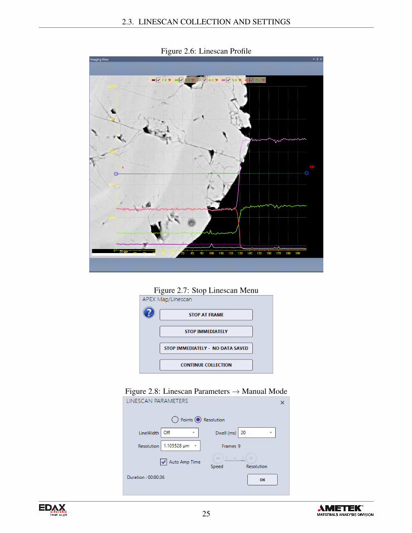
Once the line is defined, click the Collect Icon to start the linescan acquisition. The software will pre-scan the line selected and determine which elements are present, which will be shown in a pop-up boxalong with the estimated collection time. Clicking Confirm Elements in the pop-up box will immedi-ately display the detected elements on a periodic table where the user can add and remove elements asdesired. Note: If the element list is locked, a spectrum preview will not be displayed.During collection, the linescan and spectral displays are shown in real-time. The element list can bemodified and custom ROIs can be added in the same way as with mapping (described in section 2.4.1on page 30. The overlaying elements on the line can be checked or unchecked during collection toenable/disable the display of the given element. All defined elements will be displayed above the image.At the end of the scan a line profile will be displayed.To stop the linescan data collection, click the Stop icon next to the collect image icon. This can be doneat any point during the collection and the following menu of options will appear.

Stop Linescan Menu:

• Stop at Frame: Allows the collection of the current frame to complete, then stops.• Stop Immediately: Immediate stop of the collection. The data is saved for reviewing. This means

that the data collected will have dissimilar collection times before and after the point at which thecollection was stopped.

• Stop Immediately: No Data Saved: Stops the collection. There will be no data saved.• Continue Collection: Resumes the collection process. No loss of data will occur.

The right-side drop-down menu, next to the Linescan Quality Icon, allows the user to select one of thefour quality modes for data collection: Quick, SD, HD and Manual. In Quick mode the software will aimto acquire 1.000 X-rays per point on average while the numbers for SD and HD are 10.000 and 20.000respectively. The collection parameters can be customized by the user for each collection mode. To setthe linescan parameters, click the arrow next to the word Linescan on the bottom of the collection toolbarin linescan mode and a pop-up box will appear.

24

2.3. LINESCAN COLLECTION AND SETTINGS

Figure 2.6: Linescan Profile

Figure 2.7: Stop Linescan Menu

Figure 2.8: Linescan Parameters→Manual Mode

25

2.4. X-RAY MAP COLLECTION AND SETTINGS

Linescans can be acquired in two possible stepping modes: Points or Resolution. In Points mode, thenumber of points over which data will be collected is manually entered by the user. Enter the numberof points and then click Enter. In Resolution mode, select a resolution value from the drop-down list ortype in a number and the number of points used will be calculated automatically.

• LineWidth: To scan a line perpendicular to the linescan, instead of individual point locations,change the line width. This is useful for getting a more accurate intensity average for the elements.If the desired line width value is in not in the drop-down list, type in the value and press enter.

• Dwell (milliseconds): The data collection time per point per frame. If the desired dwell time isnot in the drop-down list, type in the value and press enter.

• Resolution: When using the Resolution radio button selection, this will select the distance betweeneach point collected.

• Frames: The number of integrated frames that will be collected. In manual mode, the user canselect the number of frames to collect. In the other three modes (Quick, SD or HD), the softwarewill automatically calculate the number of frames to acquire the pre-defined level of data quality.If the desired frame number is not in the drop-down list, type in the value and press enter.

• Amp Time Selection: In the automatic quality modes (Quick, SD, HD) there is a check-box forAuto Amp Time which automatically sets the amp time based on the input counts per second inorder to balance throughput and resolution. When the Manual quality icon is selected or whenAuto Amp Time is deselected in the automatic modes, the pop-up window displays a slide barwith Speed and Resolution. Drag the slide bar to one of the three locations to set amp time.

• Duration: The estimated time required to collect the linescan based on the given parameters.

2.4 X-Ray Map Collection and Settings

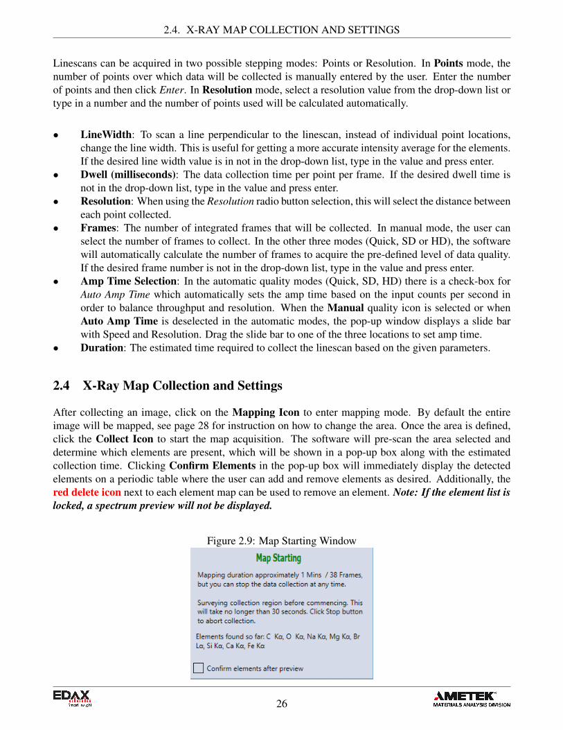
After collecting an image, click on the Mapping Icon to enter mapping mode. By default the entireimage will be mapped, see page 28 for instruction on how to change the area. Once the area is defined,click the Collect Icon to start the map acquisition. The software will pre-scan the area selected anddetermine which elements are present, which will be shown in a pop-up box along with the estimatedcollection time. Clicking Confirm Elements in the pop-up box will immediately display the detectedelements on a periodic table where the user can add and remove elements as desired. Additionally, thered delete icon next to each element map can be used to remove an element. Note: If the element list islocked, a spectrum preview will not be displayed.

Figure 2.9: Map Starting Window

26


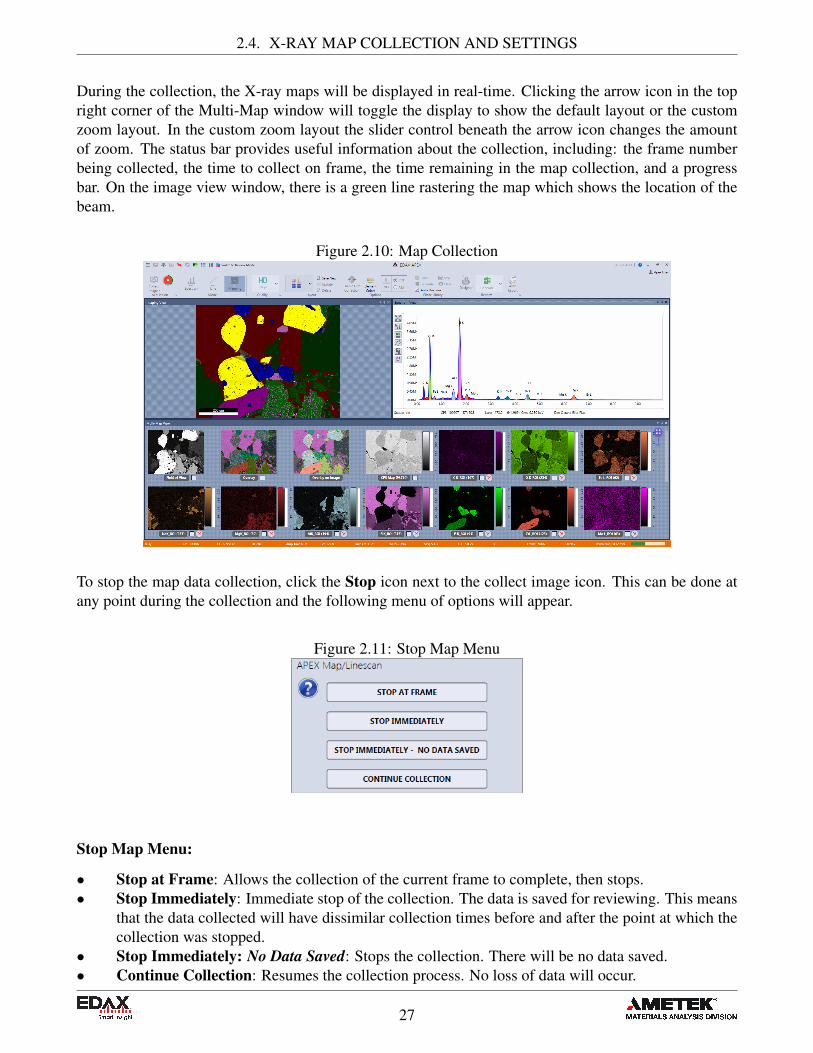
During the collection, the X-ray maps will be displayed in real-time. Clicking the arrow icon in the topright corner of the Multi-Map window will toggle the display to show the default layout or the customzoom layout. In the custom zoom layout the slider control beneath the arrow icon changes the amountof zoom. The status bar provides useful information about the collection, including: the frame numberbeing collected, the time to collect on frame, the time remaining in the map collection, and a progressbar. On the image view window, there is a green line rastering the map which shows the location of thebeam.

Figure 2.10: Map Collection

To stop the map data collection, click the Stop icon next to the collect image icon. This can be done atany point during the collection and the following menu of options will appear.

Figure 2.11: Stop Map Menu

Stop Map Menu:

• Stop at Frame: Allows the collection of the current frame to complete, then stops.• Stop Immediately: Immediate stop of the collection. The data is saved for reviewing. This means

that the data collected will have dissimilar collection times before and after the point at which thecollection was stopped.

• Stop Immediately: No Data Saved: Stops the collection. There will be no data saved.• Continue Collection: Resumes the collection process. No loss of data will occur.

27


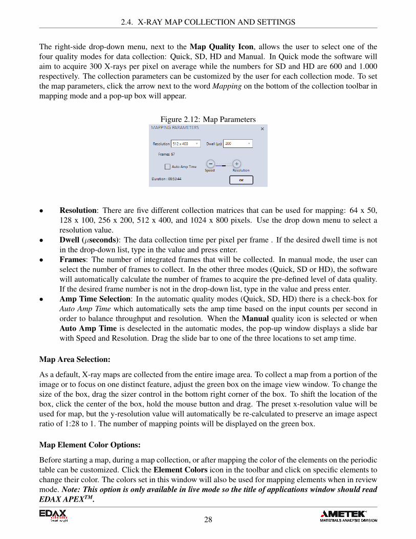
The right-side drop-down menu, next to the Map Quality Icon, allows the user to select one of thefour quality modes for data collection: Quick, SD, HD and Manual. In Quick mode the software willaim to acquire 300 X-rays per pixel on average while the numbers for SD and HD are 600 and 1.000respectively. The collection parameters can be customized by the user for each collection mode. To setthe map parameters, click the arrow next to the word Mapping on the bottom of the collection toolbar inmapping mode and a pop-up box will appear.

Figure 2.12: Map Parameters

• Resolution: There are five different collection matrices that can be used for mapping: 64 x 50,128 x 100, 256 x 200, 512 x 400, and 1024 x 800 pixels. Use the drop down menu to select aresolution value.

• Dwell (µseconds): The data collection time per pixel per frame . If the desired dwell time is notin the drop-down list, type in the value and press enter.

• Frames: The number of integrated frames that will be collected. In manual mode, the user canselect the number of frames to collect. In the other three modes (Quick, SD or HD), the softwarewill automatically calculate the number of frames to acquire the pre-defined level of data quality.If the desired frame number is not in the drop-down list, type in the value and press enter.

• Amp Time Selection: In the automatic quality modes (Quick, SD, HD) there is a check-box forAuto Amp Time which automatically sets the amp time based on the input counts per second inorder to balance throughput and resolution. When the Manual quality icon is selected or whenAuto Amp Time is deselected in the automatic modes, the pop-up window displays a slide barwith Speed and Resolution. Drag the slide bar to one of the three locations to set amp time.

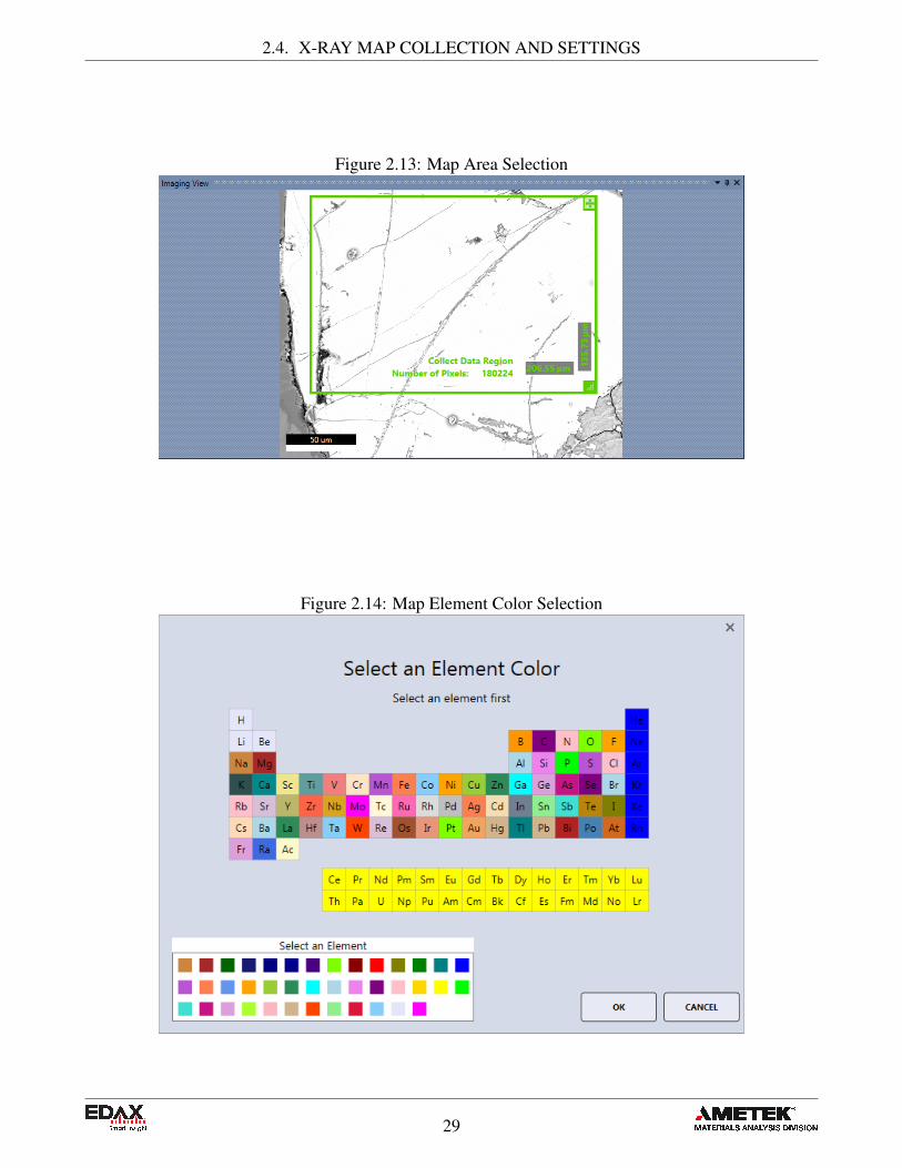
Map Area Selection:

As a default, X-ray maps are collected from the entire image area. To collect a map from a portion of theimage or to focus on one distinct feature, adjust the green box on the image view window. To change thesize of the box, drag the sizer control in the bottom right corner of the box. To shift the location of thebox, click the center of the box, hold the mouse button and drag. The preset x-resolution value will beused for map, but the y-resolution value will automatically be re-calculated to preserve an image aspectratio of 1:28 to 1. The number of mapping points will be displayed on the green box.

Map Element Color Options:

Before starting a map, during a map collection, or after mapping the color of the elements on the periodictable can be customized. Click the Element Colors icon in the toolbar and click on specific elements tochange their color. The colors set in this window will also be used for mapping elements when in reviewmode. Note: This option is only available in live mode so the title of applications window should readEDAX APEXTM.

28


Figure 2.13: Map Area Selection

Figure 2.14: Map Element Color Selection

29


2.4.1 ROI display, custom ROI and changing elements while mapping:

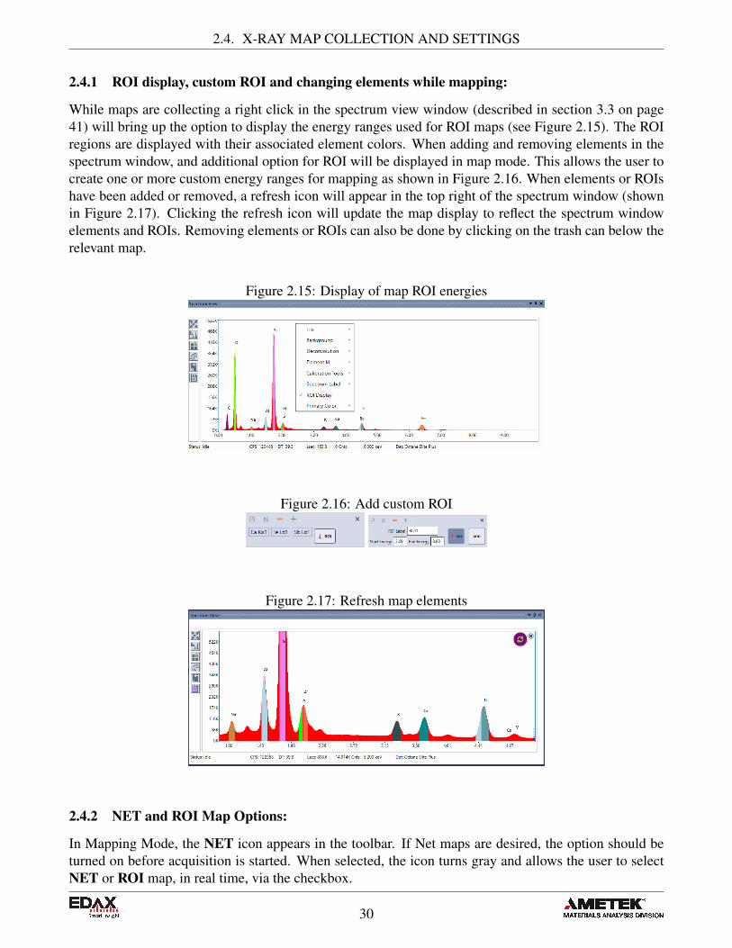
While maps are collecting a right click in the spectrum view window (described in section 3.3 on page41) will bring up the option to display the energy ranges used for ROI maps (see Figure 2.15). The ROIregions are displayed with their associated element colors. When adding and removing elements in thespectrum window, and additional option for ROI will be displayed in map mode. This allows the user tocreate one or more custom energy ranges for mapping as shown in Figure 2.16. When elements or ROIshave been added or removed, a refresh icon will appear in the top right of the spectrum window (shownin Figure 2.17). Clicking the refresh icon will update the map display to reflect the spectrum windowelements and ROIs. Removing elements or ROIs can also be done by clicking on the trash can below therelevant map.

Figure 2.15: Display of map ROI energies

Figure 2.16: Add custom ROI

Figure 2.17: Refresh map elements

2.4.2 NET and ROI Map Options:

In Mapping Mode, the NET icon appears in the toolbar. If Net maps are desired, the option should beturned on before acquisition is started. When selected, the icon turns gray and allows the user to selectNET or ROI map, in real time, via the checkbox.

30


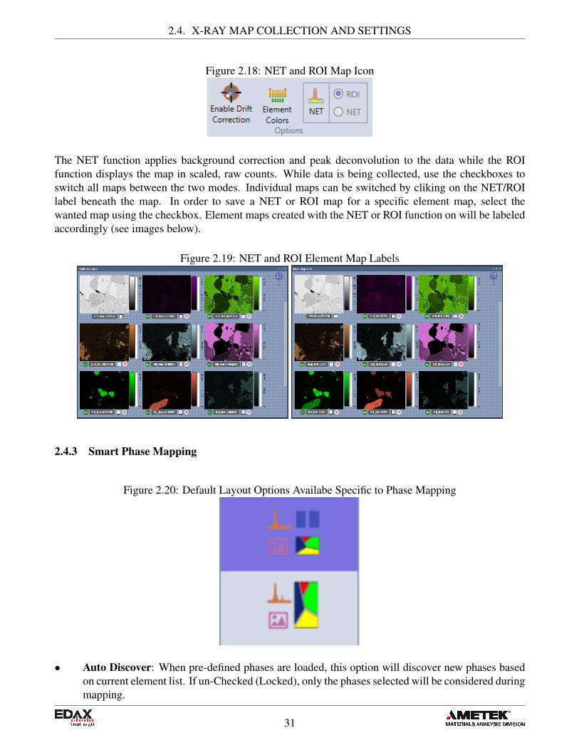
Figure 2.18: NET and ROI Map Icon

The NET function applies background correction and peak deconvolution to the data while the ROIfunction displays the map in scaled, raw counts. While data is being collected, use the checkboxes toswitch all maps between the two modes. Individual maps can be switched by cliking on the NET/ROIlabel beneath the map. In order to save a NET or ROI map for a specific element map, select thewanted map using the checkbox. Element maps created with the NET or ROI function on will be labeledaccordingly (see images below).

Figure 2.19: NET and ROI Element Map Labels

2.4.3 Smart Phase Mapping

Figure 2.20: Default Layout Options Availabe Specific to Phase Mapping

• Auto Discover: When pre-defined phases are loaded, this option will discover new phases basedon current element list. If un-Checked (Locked), only the phases selected will be considered duringmapping.

31

2.5. DRIFT CORRECTION

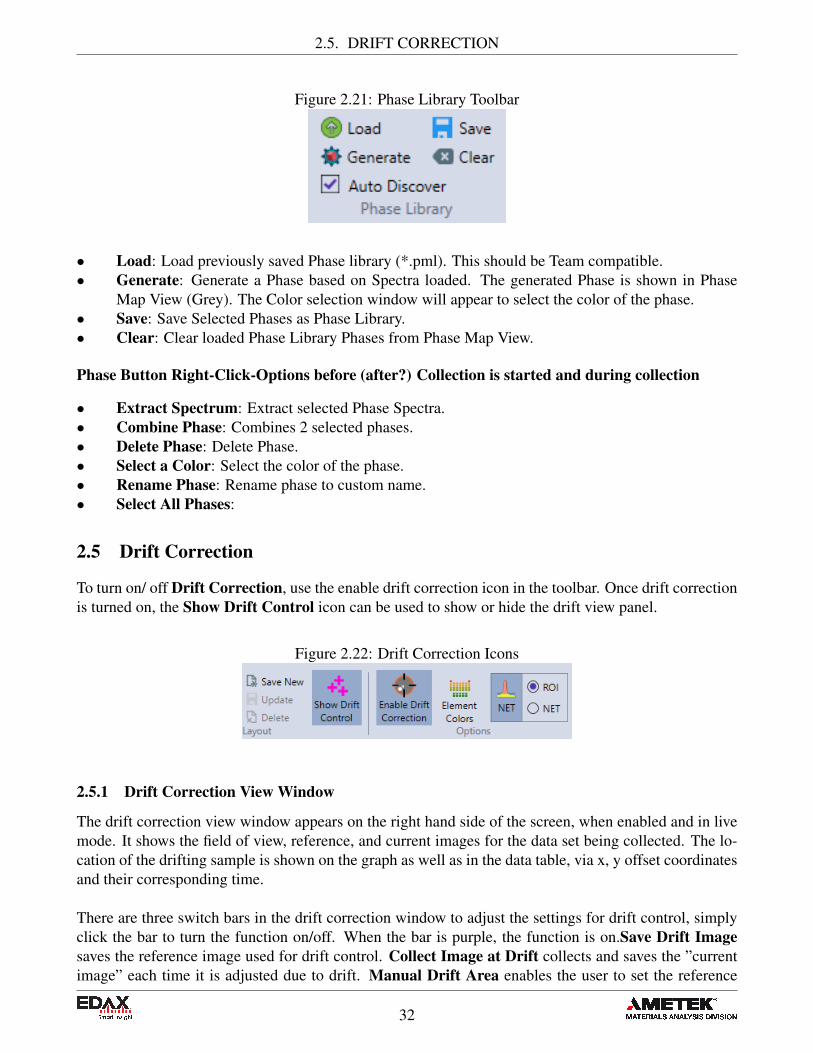
Figure 2.21: Phase Library Toolbar

• Load: Load previously saved Phase library (*.pml). This should be Team compatible.• Generate: Generate a Phase based on Spectra loaded. The generated Phase is shown in Phase

Map View (Grey). The Color selection window will appear to select the color of the phase.• Save: Save Selected Phases as Phase Library.• Clear: Clear loaded Phase Library Phases from Phase Map View.

Phase Button Right-Click-Options before (after?) Collection is started and during collection

• Extract Spectrum: Extract selected Phase Spectra.• Combine Phase: Combines 2 selected phases.• Delete Phase: Delete Phase.• Select a Color: Select the color of the phase.• Rename Phase: Rename phase to custom name.• Select All Phases:

2.5 Drift Correction

To turn on/ off Drift Correction, use the enable drift correction icon in the toolbar. Once drift correctionis turned on, the Show Drift Control icon can be used to show or hide the drift view panel.

Figure 2.22: Drift Correction Icons

2.5.1 Drift Correction View Window

The drift correction view window appears on the right hand side of the screen, when enabled and in livemode. It shows the field of view, reference, and current images for the data set being collected. The lo-cation of the drifting sample is shown on the graph as well as in the data table, via x, y offset coordinatesand their corresponding time.

There are three switch bars in the drift correction window to adjust the settings for drift control, simplyclick the bar to turn the function on/off. When the bar is purple, the function is on.Save Drift Imagesaves the reference image used for drift control. Collect Image at Drift collects and saves the ”currentimage” each time it is adjusted due to drift. Manual Drift Area enables the user to set the reference

32

2.5. DRIFT CORRECTION

Figure 2.23: The Drift Correction View Window

33

2.6. MULITIFIELD SCAN TABLE

area for drift control. When this function is turned on, before data collection starts, the user must selecta reference area on the image using the green box and click select.

Figure 2.24: Manual Drift Area

2.6 Mulitifield Scan Table

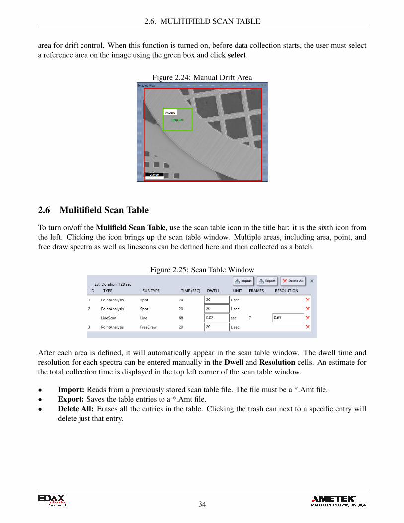
To turn on/off the Mulifield Scan Table, use the scan table icon in the title bar: it is the sixth icon fromthe left. Clicking the icon brings up the scan table window. Multiple areas, including area, point, andfree draw spectra as well as linescans can be defined here and then collected as a batch.

Figure 2.25: Scan Table Window

After each area is defined, it will automatically appear in the scan table window. The dwell time andresolution for each spectra can be entered manually in the Dwell and Resolution cells. An estimate forthe total collection time is displayed in the top left corner of the scan table window.

• Import: Reads from a previously stored scan table file. The file must be a *.Amt file.• Export: Saves the table entries to a *.Amt file.• Delete All: Erases all the entries in the table. Clicking the trash can next to a specific entry will

delete just that entry.

34

Chapter 3

Data Analysis and Display

3.1 Import, Export, and Merge Data

In bottom left corner below the project tree menu, next to the project, sample, and print icons, is theShare icon. Clicking the share icon displays a window (shown in Figure 3.2) that prompts the user withthree options: Export, Import, and Merge.Note: In live mode, clicking the share icon brings up the export window. In review mode, the export,import, and merge options are available as well.

Figure 3.1: Share Icon

Note: These icons are only visible when the project tree panel is open.

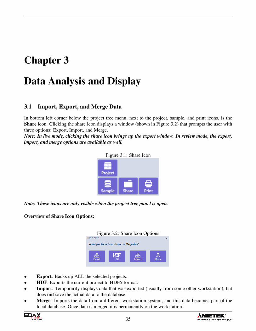
Overview of Share Icon Options:

Figure 3.2: Share Icon Options

• Export: Backs up ALL the selected projects.• HDF: Exports the current project to HDF5 format.• Import: Temporarily displays data that was exported (usually from some other workstation), but

does not save the actual data to the database.• Merge: Imports the data from a different workstation system, and this data becomes part of the

local database. Once data is merged it is permanently on the workstation.

35

3.1. IMPORT, EXPORT, AND MERGE DATA

Export Icon:

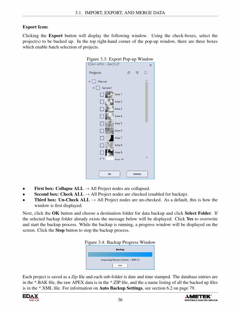
Clicking the Export button will display the following window. Using the check-boxes, select theproject(s) to be backed up. In the top right-hand corner of the pop-up window, there are three boxeswhich enable batch selection of projects.

Figure 3.3: Export Pop-up Window

• First box: Collapse ALL→ All Project nodes are collapsed.• Second box: Check ALL→ All Project nodes are checked (enabled for backup).• Third box: Un-Check ALL → All Project nodes are un-checked. As a default, this is how the

window is first displayed.

Next, click the OK button and choose a destination folder for data backup and click Select Folder. Ifthe selected backup folder already exists the message below will be displayed. Click Yes to overwriteand start the backup process. While the backup is running, a progress window will be displayed on thescreen. Click the Stop button to stop the backup process.

Figure 3.4: Backup Progress Window

Each project is saved as a Zip file and each sub-folder is date and time stamped. The database entries arein the *.BAK file, the raw APEX data is in the *.ZIP file, and the a name listing of all the backed up filesis in the *.XML file. For information on Auto Backup Settings, see section 6.2 on page 79.

36

3.2. QUANT VIEW WINDOW

Figure 3.5: Backup File Names

Import Icon:

The Import function does not permanently import data that was backed up elsewhere. This functiononly allows for the temporary review of APEXTM data: the data will not be saved on the currentworkstation. To select a *.BAK file to temporarily review, click on the project file and the progress barwill appear while the project is being restored. When it is finished, a notification will pop up, click OK.Next, the EDAX data will be loaded into the project and another progress window will appear.

Figure 3.6: Import Progress Windows

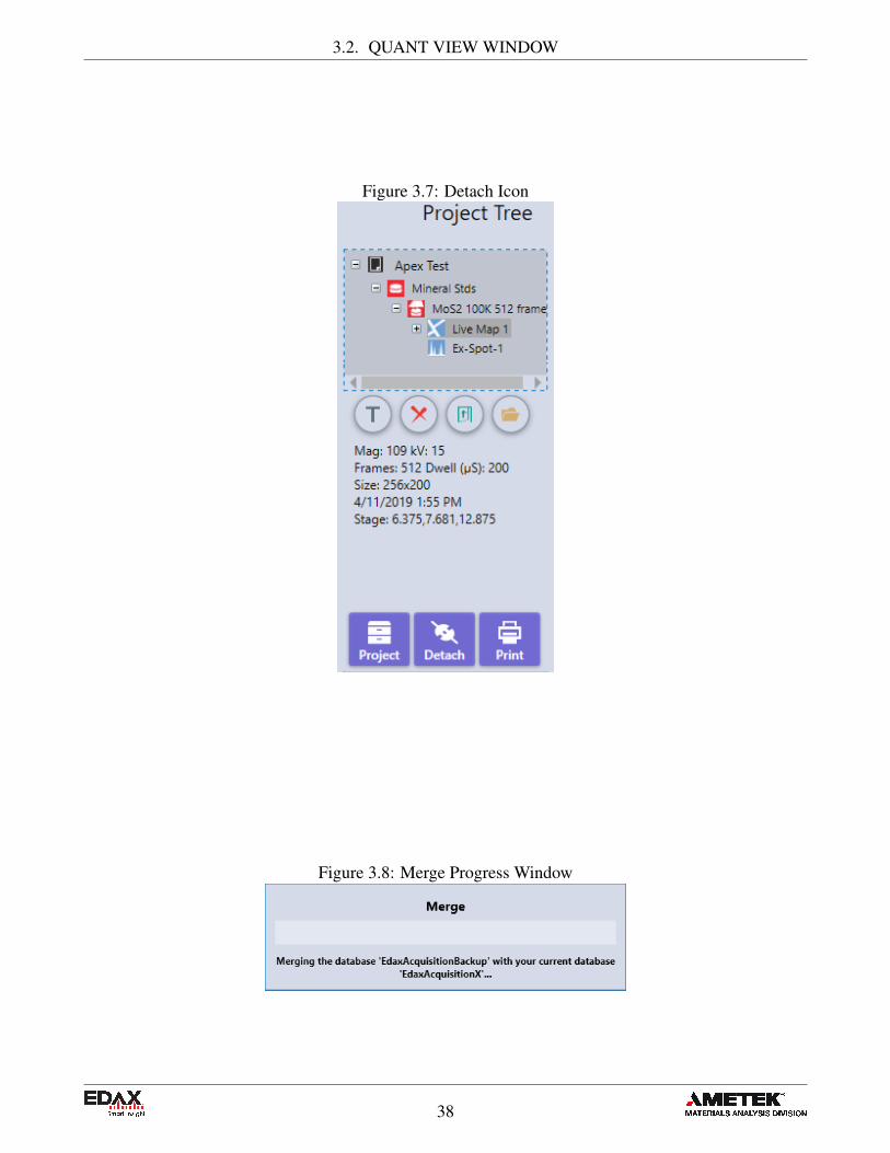
Now, the project tree is outlined with blue dashes: this is an indication that the data is only in a tempo-rary review mode. Clicking the Detach icon, on the bottom of the screen, in the center, will remove thecurrent data and switch back to selecting a project that is saved on the local computer.

Merge Icon:

To permanently import data that was backed up (via the Export icon), from another live EDAX system,click the Merge button. Select the wanted *.BAK file and the project will be merged back to the localdatabase, becoming a permanent part of the local APEXTM Database. A progress box will appear whilethe project is merging, shown in Figure 3.8. After the project has been merged, it can be found using theProject Explorer.

3.2 Quant View Window

While data is collecting, the quant results will automatically appear and update in the quant window,designated by the user in layout settings. There are multiple options for viewing quant results including:numerics only, graphs, and statistics. Be aware that any quantitative analysis requires the spectra tooriginate from a flat, homogenous bulk sample.

37


Figure 3.7: Detach Icon

Figure 3.8: Merge Progress Window

38


Numerics Only View:

The numerics only view displays the quant results in a table which can be customized by the user. Rightclick on the Quant Results Window to turn on or off (via a check mark) the quant values that will beused for display and reports. The Single Decimal Quant option sets the weight and atomic percentagesto just a single decimal point of accuracy. The default display setting is two decimal points, be awarethat this does not imply that the quant results have two decimal points of precision.

Figure 3.9: Quant Results Window and Display Options

The quant window also has a Print Menu in the upper left corner that allows the user to print or save theresults to file. To select a method, click the arrow to the right of the Print Icon to view the drop-downmenu and click on one of the following options:

Figure 3.10: Print Menu Options

• Print: Outputs the quant results to the printer.• Print→ Save (EXCEL): Outputs the quant results to a Microsoft Excel XLSX file.• Print→ Save (CSV): Outputs the quant results to an ASCII CSV file.

Note: These print options will only print the quant results, not the spectra or SEM image.

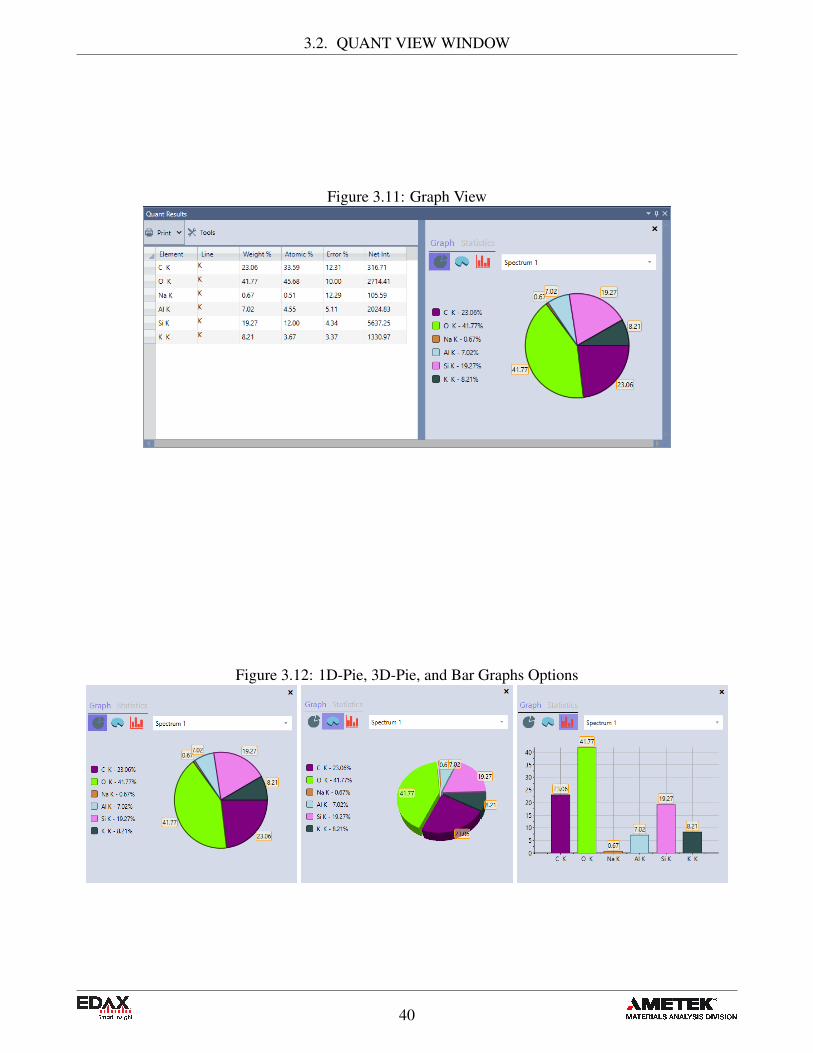
Graph View:

Clicking the Tools Icon will enable or disable the display of the weight percentage results in graphicsform. In this mode, the quant numerical values are limited to four columns. To customize which resultsare displayed, right click on the quant results window.There are three graph display modes: 1D-Pie, 3D-Pie, and Bar Graph. To select a mode, use the iconsunder the word Graph. When using the bar graph mode, there is a drop-down selection. When multiplespectra are loaded, the user can quickly switch between the quant graphs of each spectrum using the dropdown menu above the graph.

39


Figure 3.11: Graph View

Figure 3.12: 1D-Pie, 3D-Pie, and Bar Graphs Options

40

3.3. SPECTRUM VIEW WINDOW

Statistics View:

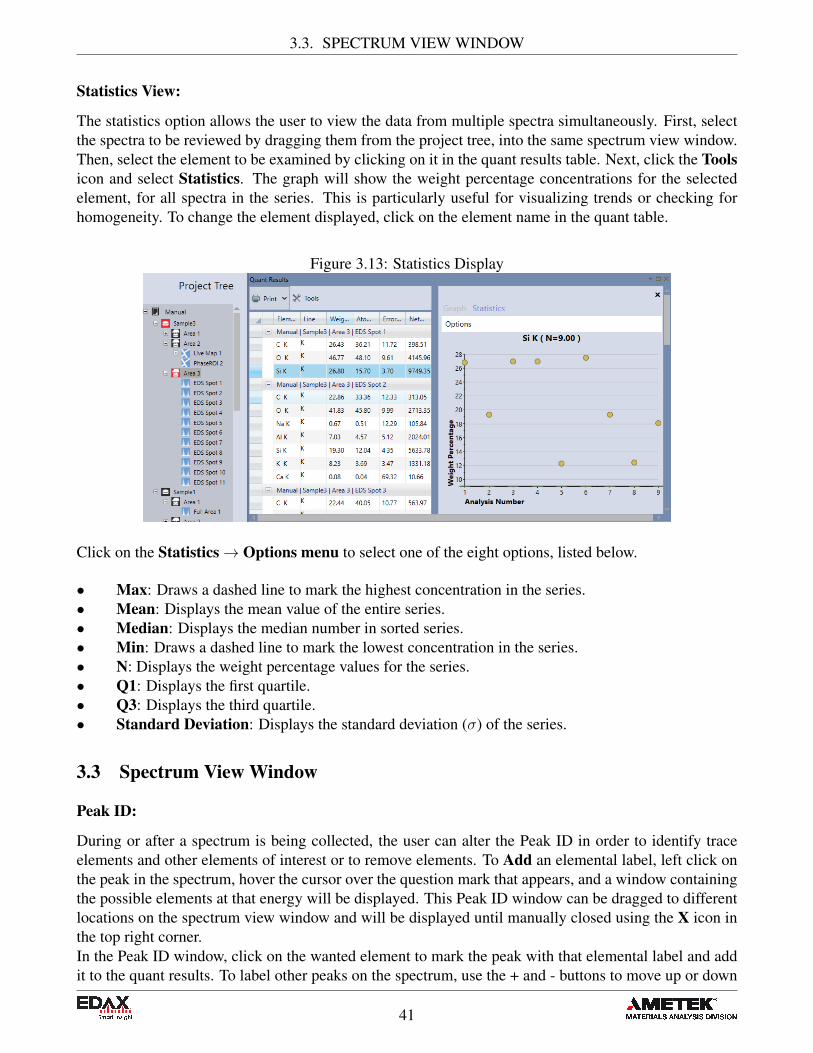
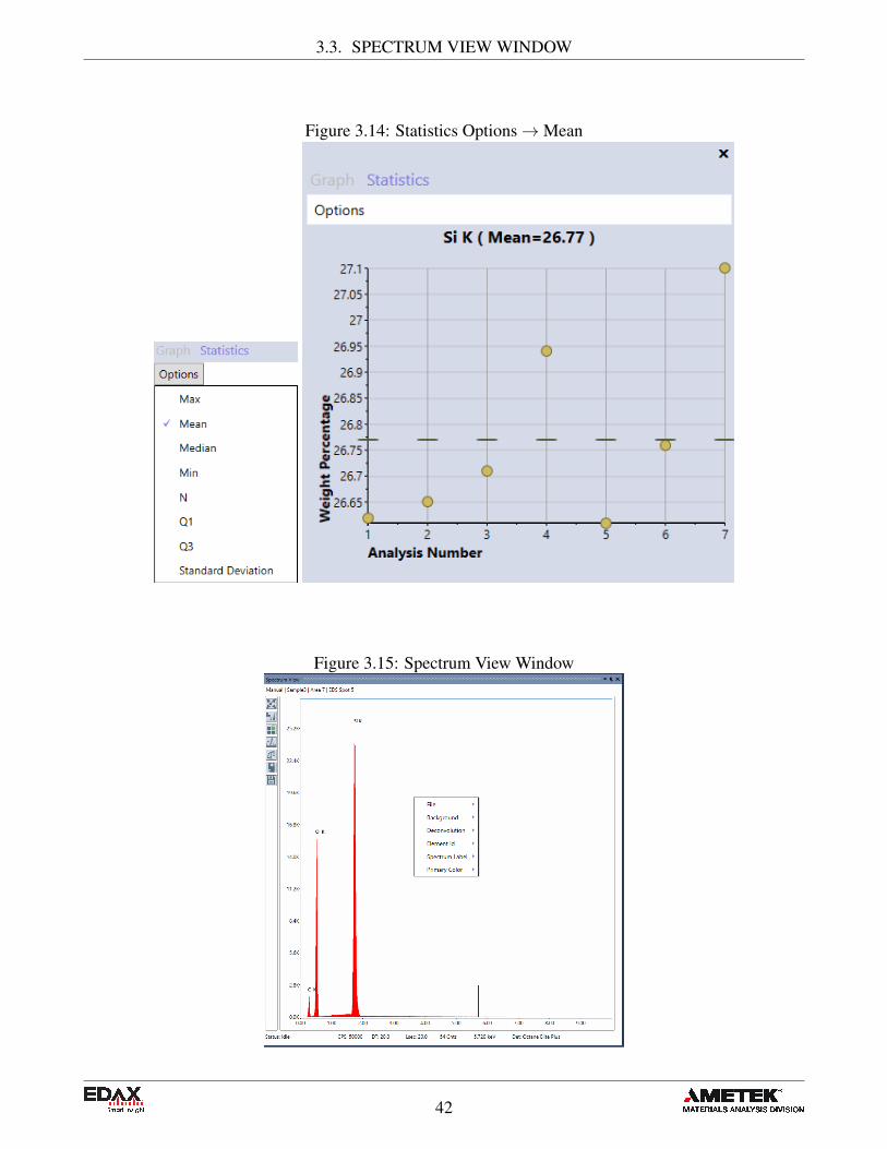
The statistics option allows the user to view the data from multiple spectra simultaneously. First, selectthe spectra to be reviewed by dragging them from the project tree, into the same spectrum view window.Then, select the element to be examined by clicking on it in the quant results table. Next, click the Toolsicon and select Statistics. The graph will show the weight percentage concentrations for the selectedelement, for all spectra in the series. This is particularly useful for visualizing trends or checking forhomogeneity. To change the element displayed, click on the element name in the quant table.

Figure 3.13: Statistics Display

Click on the Statistics→ Options menu to select one of the eight options, listed below.

• Max: Draws a dashed line to mark the highest concentration in the series.• Mean: Displays the mean value of the entire series.• Median: Displays the median number in sorted series.• Min: Draws a dashed line to mark the lowest concentration in the series.• N: Displays the weight percentage values for the series.• Q1: Displays the first quartile.• Q3: Displays the third quartile.• Standard Deviation: Displays the standard deviation (σ) of the series.

3.3 Spectrum View Window

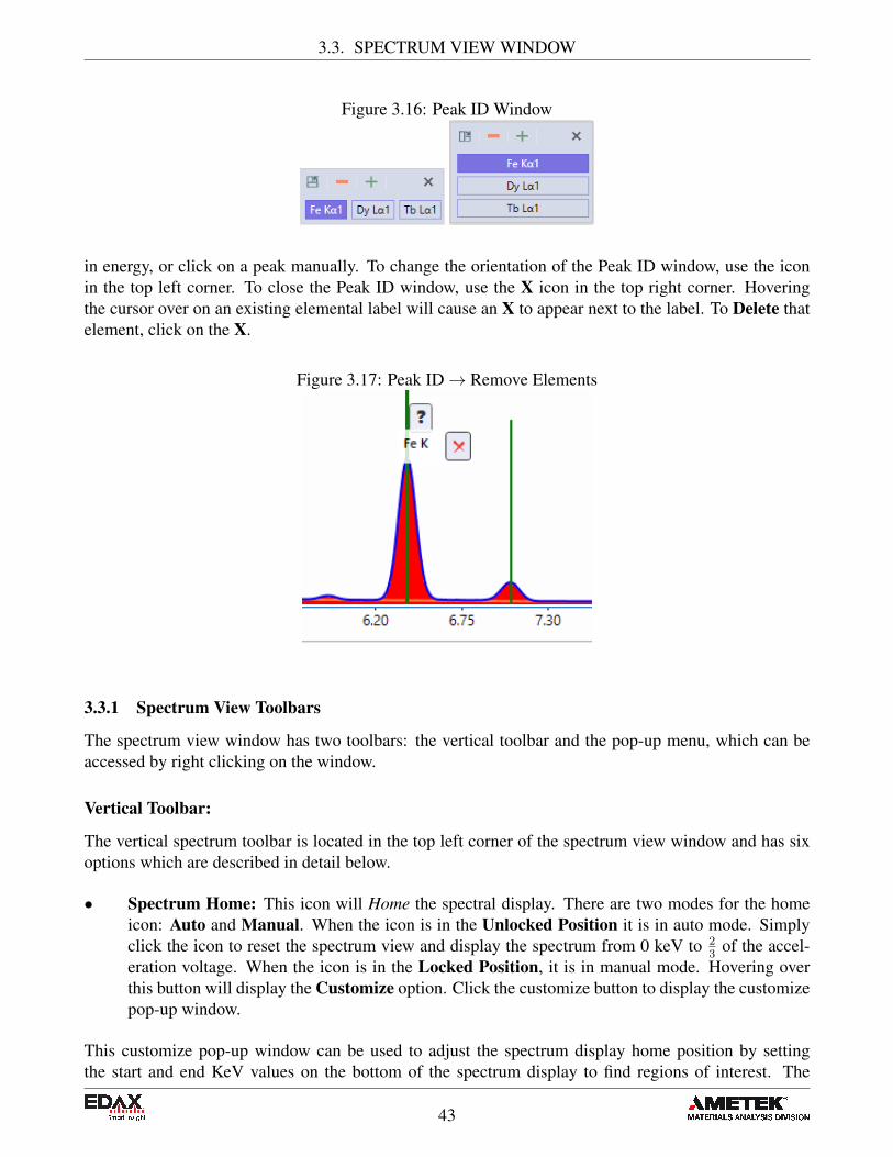
Peak ID:

During or after a spectrum is being collected, the user can alter the Peak ID in order to identify traceelements and other elements of interest or to remove elements. To Add an elemental label, left click onthe peak in the spectrum, hover the cursor over the question mark that appears, and a window containingthe possible elements at that energy will be displayed. This Peak ID window can be dragged to differentlocations on the spectrum view window and will be displayed until manually closed using the X icon inthe top right corner.In the Peak ID window, click on the wanted element to mark the peak with that elemental label and addit to the quant results. To label other peaks on the spectrum, use the + and - buttons to move up or down

41


Figure 3.14: Statistics Options→Mean

Figure 3.15: Spectrum View Window

42


Figure 3.16: Peak ID Window

in energy, or click on a peak manually. To change the orientation of the Peak ID window, use the iconin the top left corner. To close the Peak ID window, use the X icon in the top right corner. Hoveringthe cursor over on an existing elemental label will cause an X to appear next to the label. To Delete thatelement, click on the X.

Figure 3.17: Peak ID→ Remove Elements

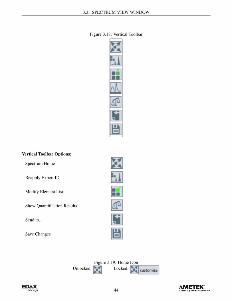
3.3.1 Spectrum View Toolbars

The spectrum view window has two toolbars: the vertical toolbar and the pop-up menu, which can beaccessed by right clicking on the window.

Vertical Toolbar:

The vertical spectrum toolbar is located in the top left corner of the spectrum view window and has sixoptions which are described in detail below.

• Spectrum Home: This icon will Home the spectral display. There are two modes for the homeicon: Auto and Manual. When the icon is in the Unlocked Position it is in auto mode. Simplyclick the icon to reset the spectrum view and display the spectrum from 0 keV to 2

3of the accel-

eration voltage. When the icon is in the Locked Position, it is in manual mode. Hovering overthis button will display the Customize option. Click the customize button to display the customizepop-up window.

This customize pop-up window can be used to adjust the spectrum display home position by settingthe start and end KeV values on the bottom of the spectrum display to find regions of interest. The

43


Figure 3.18: Vertical Toolbar

Vertical Toolbar Options:

Spectrum Home

Reapply Expert ID

Modify Element List

Show Quantification Results

Send to...

Save Changes

Figure 3.19: Home IconUnlocked: Locked:

44


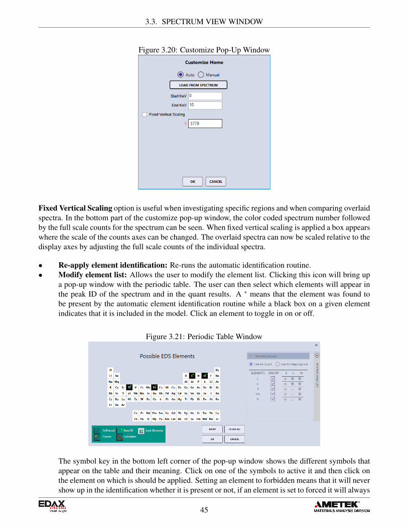
Figure 3.20: Customize Pop-Up Window

Fixed Vertical Scaling option is useful when investigating specific regions and when comparing overlaidspectra. In the bottom part of the customize pop-up window, the color coded spectrum number followedby the full scale counts for the spectrum can be seen. When fixed vertical scaling is applied a box appearswhere the scale of the counts axes can be changed. The overlaid spectra can now be scaled relative to thedisplay axes by adjusting the full scale counts of the individual spectra.

• Re-apply element identification: Re-runs the automatic identification routine.• Modify element list: Allows the user to modify the element list. Clicking this icon will bring up

a pop-up window with the periodic table. The user can then select which elements will appear inthe peak ID of the spectrum and in the quant results. A ∗ means that the element was found tobe present by the automatic element identification routine while a black box on a given elementindicates that it is included in the model. Click an element to toggle in on or off.

Figure 3.21: Periodic Table Window

The symbol key in the bottom left corner of the pop-up window shows the different symbols thatappear on the table and their meaning. Click on one of the symbols to active it and then click onthe element on which is should be applied. Setting an element to forbidden means that it will nevershow up in the identification whether it is present or not, if an element is set to forced it will always

45


show up in the identification whether it is present or not, Setting an element to unforced meansthat it is included in the model but can potentially be removed on subsequent applications of theautomatic identification if it is not found to be present. This pop-up window also gives the userthe option to lock or unlock the elements used for peak ID. When the element list is unlocked, thesymbol is green. When the element list is locked, the symbol is red. Clicking the← on the righthand side of the window expands the ZAF list control which enables the user to select the energylines used to quantify and map each element.

• Show Quantification Results: This icon displays the quant results in a pop-up window. Since thequant results are displayed in the quant window, in real-time, during its collection, this icon is onlyneeded for certain layout options.

• Send to... This icon has three options for sending or saving the current files:

• Send to Folder: Sends the following files to the folder defined in user preferences: SPC (Bi-nary Spectrum File), MSA, CSV, *.BMP (or other image file depending on user preferencesetting).

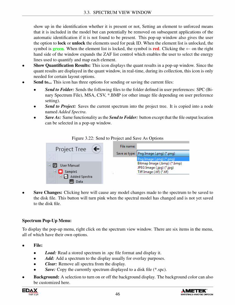
• Send to Project: Saves the current spectrum into the project tree. It is copied into a nodenamed Added Spectra.

• Save As: Same functionality as the Send to Folder: button except that the file output locationcan be selected in a pop-up window.

Figure 3.22: Send to Project and Save As Options

• Save Changes: Clicking here will cause any model changes made to the spectrum to be saved tothe disk file. This button will turn pink when the spectral model has changed and is not yet savedto the disk file.

Spectrum Pop-Up Menu:

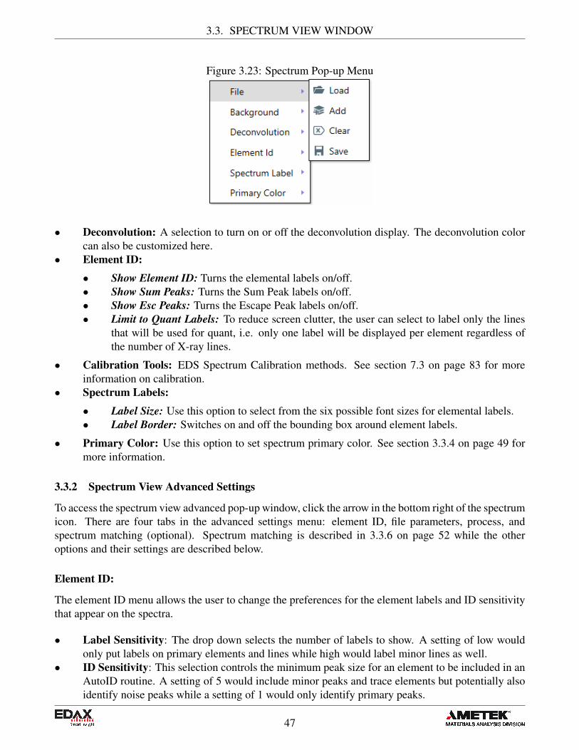
To display the pop-up menu, right click on the spectrum view window. There are six items in the menu,all of which have their own options.

• File:• Load: Read a stored spectrum in .spc file format and display it.• Add: Add a spectrum to the display usually for overlay purposes.• Clear: Remove all spectra from the display.• Save: Copy the currently spectrum displayed to a disk file (*.spc).

• Background: A selection to turn on or off the background display. The background color can alsobe customized here.

46


Figure 3.23: Spectrum Pop-up Menu

• Deconvolution: A selection to turn on or off the deconvolution display. The deconvolution colorcan also be customized here.

• Element ID:

• Show Element ID: Turns the elemental labels on/off.• Show Sum Peaks: Turns the Sum Peak labels on/off.• Show Esc Peaks: Turns the Escape Peak labels on/off.• Limit to Quant Labels: To reduce screen clutter, the user can select to label only the lines

that will be used for quant, i.e. only one label will be displayed per element regardless ofthe number of X-ray lines.

• Calibration Tools: EDS Spectrum Calibration methods. See section 7.3 on page 83 for moreinformation on calibration.

• Spectrum Labels:

• Label Size: Use this option to select from the six possible font sizes for elemental labels.• Label Border: Switches on and off the bounding box around element labels.

• Primary Color: Use this option to set spectrum primary color. See section 3.3.4 on page 49 formore information.

3.3.2 Spectrum View Advanced Settings

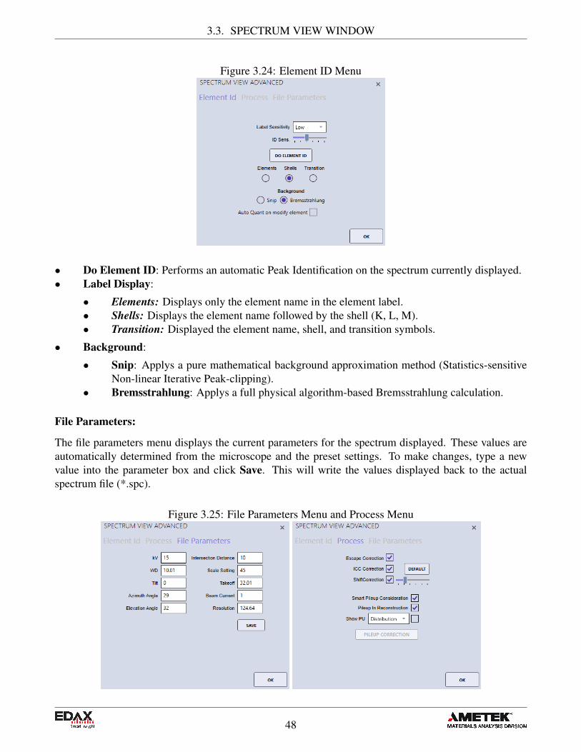
To access the spectrum view advanced pop-up window, click the arrow in the bottom right of the spectrumicon. There are four tabs in the advanced settings menu: element ID, file parameters, process, andspectrum matching (optional). Spectrum matching is described in 3.3.6 on page 52 while the otheroptions and their settings are described below.

Element ID:

The element ID menu allows the user to change the preferences for the element labels and ID sensitivitythat appear on the spectra.

• Label Sensitivity: The drop down selects the number of labels to show. A setting of low wouldonly put labels on primary elements and lines while high would label minor lines as well.

• ID Sensitivity: This selection controls the minimum peak size for an element to be included in anAutoID routine. A setting of 5 would include minor peaks and trace elements but potentially alsoidentify noise peaks while a setting of 1 would only identify primary peaks.

47


Figure 3.24: Element ID Menu

• Do Element ID: Performs an automatic Peak Identification on the spectrum currently displayed.• Label Display:

• Elements: Displays only the element name in the element label.• Shells: Displays the element name followed by the shell (K, L, M).• Transition: Displayed the element name, shell, and transition symbols.

• Background:

• Snip: Applys a pure mathematical background approximation method (Statistics-sensitiveNon-linear Iterative Peak-clipping).

• Bremsstrahlung: Applys a full physical algorithm-based Bremsstrahlung calculation.

File Parameters:

The file parameters menu displays the current parameters for the spectrum displayed. These values areautomatically determined from the microscope and the preset settings. To make changes, type a newvalue into the parameter box and click Save. This will write the values displayed back to the actualspectrum file (*.spc).

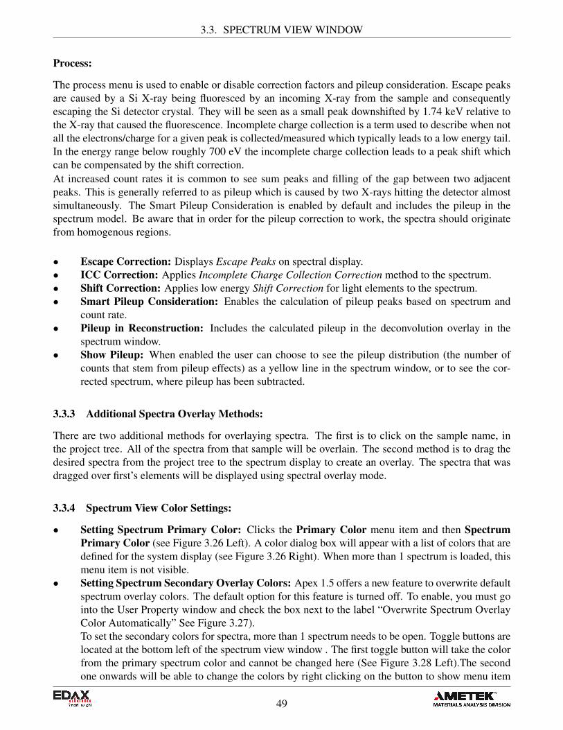
Figure 3.25: File Parameters Menu and Process Menu

48


Process:

The process menu is used to enable or disable correction factors and pileup consideration. Escape peaksare caused by a Si X-ray being fluoresced by an incoming X-ray from the sample and consequentlyescaping the Si detector crystal. They will be seen as a small peak downshifted by 1.74 keV relative tothe X-ray that caused the fluorescence. Incomplete charge collection is a term used to describe when notall the electrons/charge for a given peak is collected/measured which typically leads to a low energy tail.In the energy range below roughly 700 eV the incomplete charge collection leads to a peak shift whichcan be compensated by the shift correction.At increased count rates it is common to see sum peaks and filling of the gap between two adjacentpeaks. This is generally referred to as pileup which is caused by two X-rays hitting the detector almostsimultaneously. The Smart Pileup Consideration is enabled by default and includes the pileup in thespectrum model. Be aware that in order for the pileup correction to work, the spectra should originatefrom homogenous regions.

• Escape Correction: Displays Escape Peaks on spectral display.• ICC Correction: Applies Incomplete Charge Collection Correction method to the spectrum.• Shift Correction: Applies low energy Shift Correction for light elements to the spectrum.• Smart Pileup Consideration: Enables the calculation of pileup peaks based on spectrum and

count rate.• Pileup in Reconstruction: Includes the calculated pileup in the deconvolution overlay in the

spectrum window.• Show Pileup: When enabled the user can choose to see the pileup distribution (the number of

counts that stem from pileup effects) as a yellow line in the spectrum window, or to see the cor-rected spectrum, where pileup has been subtracted.

3.3.3 Additional Spectra Overlay Methods:

There are two additional methods for overlaying spectra. The first is to click on the sample name, inthe project tree. All of the spectra from that sample will be overlain. The second method is to drag thedesired spectra from the project tree to the spectrum display to create an overlay. The spectra that wasdragged over first’s elements will be displayed using spectral overlay mode.

3.3.4 Spectrum View Color Settings:

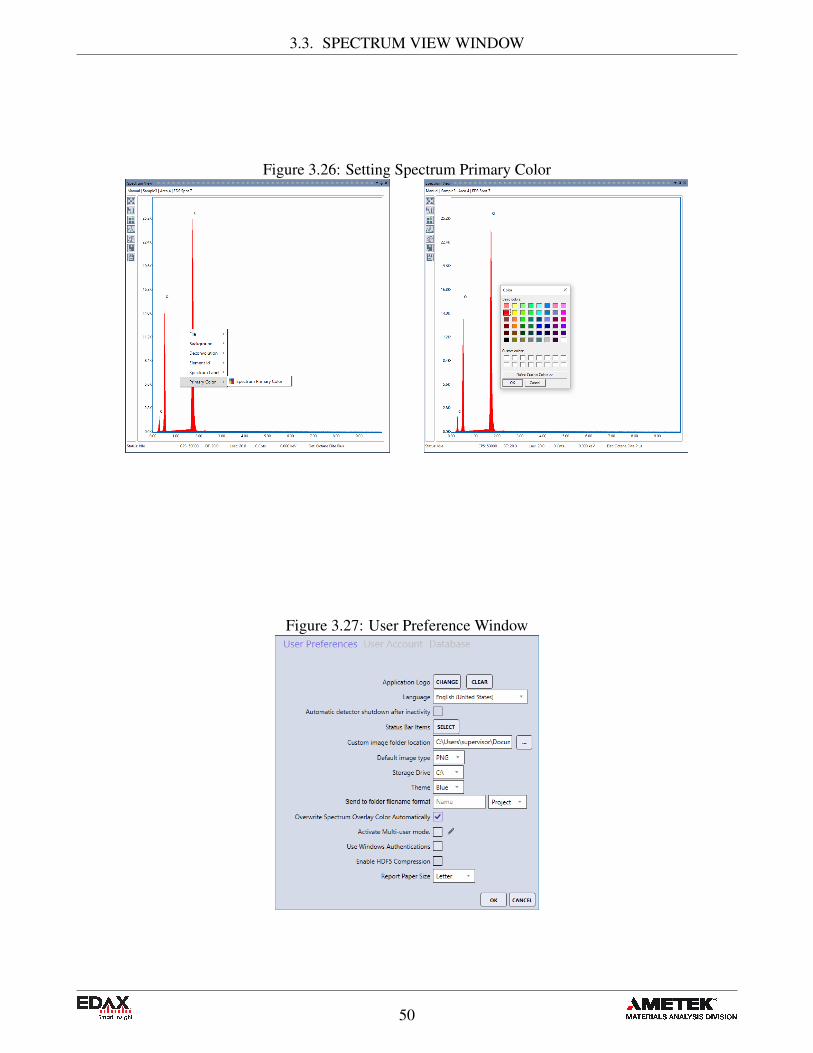
• Setting Spectrum Primary Color: Clicks the Primary Color menu item and then SpectrumPrimary Color (see Figure 3.26 Left). A color dialog box will appear with a list of colors that aredefined for the system display (see Figure 3.26 Right). When more than 1 spectrum is loaded, thismenu item is not visible.

• Setting Spectrum Secondary Overlay Colors: Apex 1.5 offers a new feature to overwrite defaultspectrum overlay colors. The default option for this feature is turned off. To enable, you must gointo the User Property window and check the box next to the label “Overwrite Spectrum OverlayColor Automatically” See Figure 3.27).To set the secondary colors for spectra, more than 1 spectrum needs to be open. Toggle buttons arelocated at the bottom left of the spectrum view window . The first toggle button will take the colorfrom the primary spectrum color and cannot be changed here (See Figure 3.28 Left).The secondone onwards will be able to change the colors by right clicking on the button to show menu item

49


Figure 3.26: Setting Spectrum Primary Color

Figure 3.27: User Preference Window

50


“Change Overlay color”. Right click on the toggle button to change overlay color for the spectrum(See Figure 3.28 Right).

• Closing a Spectrum when Multi-spectra are Opened: To close a spectrum, right click on thetoggle button and click Close Spectrum button (See Figure 3.28 Right).

Figure 3.28: Setting Spectrum Secondary Overlay Colors

3.3.5 Multi-spectra View

Whenever there is more than one spectra loaded, there is feature that can open each spectrum into aMulti-Spectra View. To use this feature, right click on the spectrum view window to open the contextmenu. Click the menu item “Explode”, this will open the Multi-Spectra View. (See Figure 3.29)

Figure 3.29: Explode Menu Item

There are three view modes available on the Multi-Spectra view window (see Figure 3.30).

• List View:this view will display all spectra vertically (see Figure 3.31).• Carousel view: A carousel view provides scrolling animation to create the effect of a spec-

trum movement when scrolled. This view has four predefined configuration: Diagonal, Ellipse,Parabola, and Zigzag (see Figure 3.32).

51


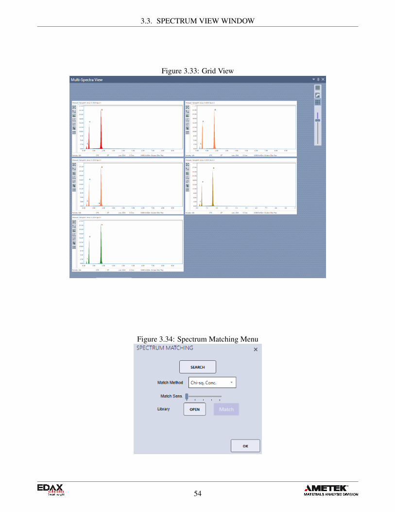
• Grid View: this view arranges each spectrum from left to right based on available space. There isa zoom control to resize each spectrum (see Figure 3.33).

Figure 3.30: View Modes

Figure 3.31: List View

3.3.6 Spectrum Matching (Optional):

• Match Method: There are two types of matching possible, Chi-Squared fit on Concentration oron the Raw Spectral Channel Data. Use the drop-down menu to select a method.

52


Figure 3.32: Carousel View

• Match Sensitivity: The minimum fit threshold required to report a match to the unknown. Ad-justed the threshold by using the slider bar to set a percentage.

• Library→Open: Use this option to load a saved spectrum match library file. Click open andselect a file from the local computer.

• Library→Match: Runs a spectrum matching search using the currently defined match library forthe best possible matches against the currently displayed spectrum. The spectrum matches will bedisplayed in overlay on the spectrum display. The name of the currently loaded spectrum matchlibrary file will be displayed below the open/ match icons.

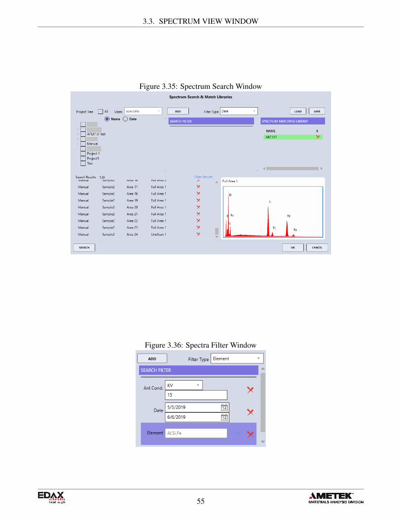
• Search: Displays a setup window for defining, reviewing or modifying a match library file. Toload an existing match library double click on the name in the spectrum matching library panel, orclick on the name and then the Load button. To create a new library or modify an existing selectthe project(s) or project nodes that contain the desired match spectra and click the Search buttonat the bottom left of the window. This will populate the search result list, where individual spectracan be selected to display them in the mini-spectrum view. Spectra can be removed from the listby the delete button. Once the list is complete, the library can be saved by clicking on the Savebutton. If desired, a filter can be added to the search via the Add button above the search window.There are three filter types for searching: Date, Element, and Analysis conditions. After settinga new search filter, click Search.

• Date: Allows the user to filter search results based on the spectra date. The start and end date mustbe provided.

• Element: Allows the user to filter search results based on the elements in the spectra. Seebelow for details.

53


Figure 3.33: Grid View

Figure 3.34: Spectrum Matching Menu

54


Figure 3.35: Spectrum Search Window

Figure 3.36: Spectra Filter Window

55

3.4. LINESCAN VIEW→ IMAGE WINDOW

• Analysis Conditions: Allows the user to filter search results based on the kV or name ofthe spectra.

When in Element mode, clicking the Add button brings up a pop-up window that allows the userto define which elements to filter search results based on by using the periodic table and input theelemental concentration or intensity min/max range.

Figure 3.37: Element Search Pop-Up Window

After the spectra have been selected and the preferences for spectrum matching have been set, click theMatch button in the spectrum matching menu. The software will perform the matching process to theactive spectrum that is currently displayed. The first three spectra from the match library file will bedisplayed overlaid the original spectrum. In the top right of the main spectrum window, the names of thematched spectra and their matched fit percentage, set by the match sensitivity option, are displayed.

3.4 Linescan View→ Image Window

When in linescan mode, the spectral lines of each element appear in the image window, overlaid on theimage. The user can check or uncheck the boxes on the top of the image to display the profiles of eachelement.In the image below, all elements have been unchecked except the Fe K profile, therefore; only the Fe Kis now displayed. To send the image to the folder defined in User Preferences, right click on the imageand select Send to Folder.

3.5 Multi-Map View Window

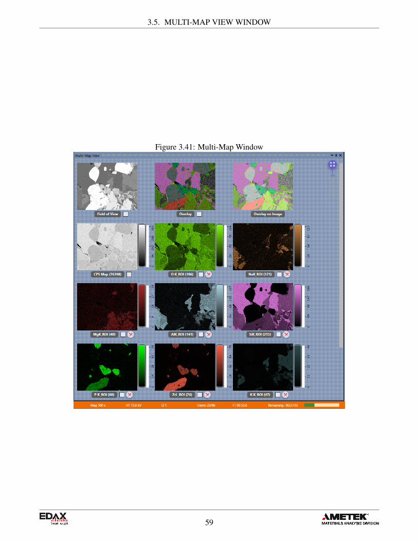
When in mapping mode, the Multi-Map View window displays the different types of maps that thesoftware compiles, as thumbnails in the same window. The name, data type (Field of View/SEM image,

56

3.5. MULTI-MAP VIEW WINDOW

Figure 3.38: Spectrum Matching Overlay

Figure 3.39: Linescan View

57


Figure 3.40: Linescan View: One Element

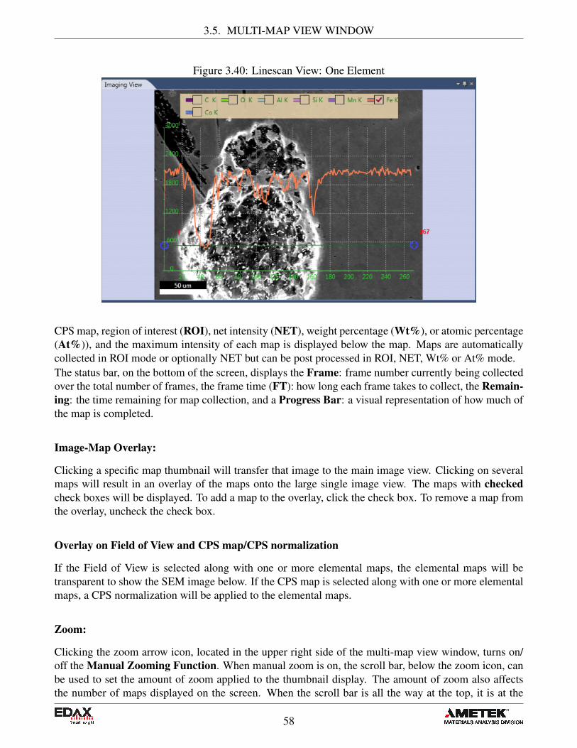
CPS map, region of interest (ROI), net intensity (NET), weight percentage (Wt%), or atomic percentage(At%)), and the maximum intensity of each map is displayed below the map. Maps are automaticallycollected in ROI mode or optionally NET but can be post processed in ROI, NET, Wt% or At% mode.The status bar, on the bottom of the screen, displays the Frame: frame number currently being collectedover the total number of frames, the frame time (FT): how long each frame takes to collect, the Remain-ing: the time remaining for map collection, and a Progress Bar: a visual representation of how much ofthe map is completed.

Image-Map Overlay:

Clicking a specific map thumbnail will transfer that image to the main image view. Clicking on severalmaps will result in an overlay of the maps onto the large single image view. The maps with checkedcheck boxes will be displayed. To add a map to the overlay, click the check box. To remove a map fromthe overlay, uncheck the check box.

Overlay on Field of View and CPS map/CPS normalization

If the Field of View is selected along with one or more elemental maps, the elemental maps will betransparent to show the SEM image below. If the CPS map is selected along with one or more elementalmaps, a CPS normalization will be applied to the elemental maps.

Zoom:

Clicking the zoom arrow icon, located in the upper right side of the multi-map view window, turns on/off the Manual Zooming Function. When manual zoom is on, the scroll bar, below the zoom icon, canbe used to set the amount of zoom applied to the thumbnail display. The amount of zoom also affectsthe number of maps displayed on the screen. When the scroll bar is all the way at the top, it is at the

58


Figure 3.41: Multi-Map Window

59

3.6. MAPPING POP-UP MENU:

maximum zoom factor and only one map will be displayed. Depending on the amount of zoom applied,there is a vertical scale Intensity Bar to the right of each map showing its corresponding intensity scale.

3.6 Mapping Pop-Up Menu:

To display the Mapping Pop-up Menu, right click on any of the maps. The menu has three mainfunctions: Map Scaling, Palettes, and Send to Folder. The functions and their options are explainedbelow.

Map Scaling:

Map scaling enables the user to select a range of values, based on the collected intensities, for the mapdisplay.

Figure 3.42: Map Scaling Menu Options

• Apply All: When checked, the intensity settings will be applied to all maps in the display.• Selected Region: Allows the user to define a low and high threshold in the histogram to extract a

spectrum from. See below for histogram details.• Auto Enhance: Suppresses hot and cold pixels and enhances contrast by using 95% of the total

histogram data for display. The intensity bar advanced options are not accessible in auto enhancemode. See below for intensity bar advanced options.

• Manual: Allows the user to manually adjust the intensity of one map.• Manual All: Applies the manually set intensity value to all maps. This mode is most useful for

quantitative maps where all maps can be scaled to one value.

Intensity Bar Advanced

: In modes other than Auto Enhance Mode, the vertical intensity bar changes to display more advancedfeatures. There are two red arrow sliders and two grey round sliders to select other optional modes. Thered sliders are used to adjust the contrast of the map. The contrast of the map below has been adjustedby lowering the upper red slider. The left map’s upper slider is at a value of 86 counts while the right’sis at 21 counts.

Histogram Settings

: The histogram used for spectrum extraction is compiled by sorting map pixels based on their intensity.These intensities are then normalized and displayed as a histogram. Clicking the Bottom Grey RoundButton will display the histogram of the map data. Clicking on the button again (which is now rainbowcolored), will Close the histogram window.

60


Figure 3.43: Intensity Bar Advanced: Contrast Adjustment

Figure 3.44: Histogram Display

Below the histogram, the upper and lower threshold values for spectrum extracted can be entered. Afterentering a range of values, the data range and fraction of the total area selected will be displayed. ClickExtract Spectrum to apply these values. To reset the threshold values, click Reset Area. Clicking theupper gray round button will extract and display the map’s Intensity Range Spectrum. The range ofvalues is displayed in the title bar of the spectrum.

Palettes:

The palette function allows the user to set the color palette to one of the two options: Color and Thermal.

• Apply All: When checked, the currently defined palette settings will be applied to all maps in thedisplay. To define specific maps to the current palette, uncheck this option.

• Color: Displays maps using 256 shades of a single color.• Thermal: Displays maps using a standard thermal palette with 256 shades between black and

white.

Send to Folder:

The Send to Folder option sends the currently selected image or map to the folder specified in the userpreferences window. The map is saved as an image and .csv file.

61


Figure 3.45: Intensity Range Spectrum

Figure 3.46: Map Scaling Menu Options

Figure 3.47: Color vs. Thermal Palette

62

Chapter 4

Review Mode and Toolbars

After data has been collected using one of the three collection modes, it can be reviewed and revised inreview mode. To enter review mode, click the Switch to Review Mode icon in the title bar toolbar.

4.1 Spectrum Review

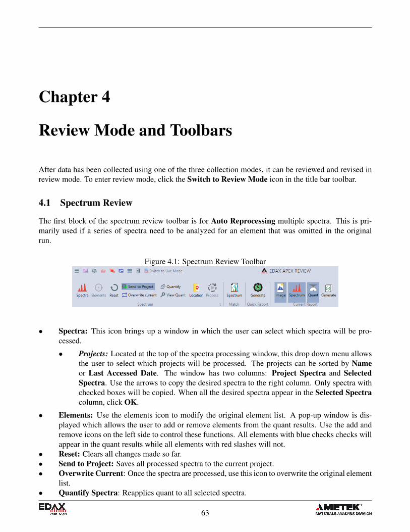
The first block of the spectrum review toolbar is for Auto Reprocessing multiple spectra. This is pri-marily used if a series of spectra need to be analyzed for an element that was omitted in the originalrun.

Figure 4.1: Spectrum Review Toolbar

• Spectra: This icon brings up a window in which the user can select which spectra will be pro-cessed.

• Projects: Located at the top of the spectra processing window, this drop down menu allowsthe user to select which projects will be processed. The projects can be sorted by Nameor Last Accessed Date. The window has two columns: Project Spectra and SelectedSpectra. Use the arrows to copy the desired spectra to the right column. Only spectra withchecked boxes will be copied. When all the desired spectra appear in the Selected Spectracolumn, click OK.

• Elements: Use the elements icon to modify the original element list. A pop-up window is dis-played which allows the user to add or remove elements from the quant results. Use the add andremove icons on the left side to control these functions. All elements with blue checks checks willappear in the quant results while all elements with red slashes will not.

• Reset: Clears all changes made so far.• Send to Project: Saves all processed spectra to the current project.• Overwrite Current: Once the spectra are processed, use this icon to overwrite the original element

list.• Quantify Spectra: Reapplies quant to all selected spectra.

63

4.1. SPECTRUM REVIEW

Figure 4.2: Spectra Processing Window

Figure 4.3: Elements Pop-up Window

64

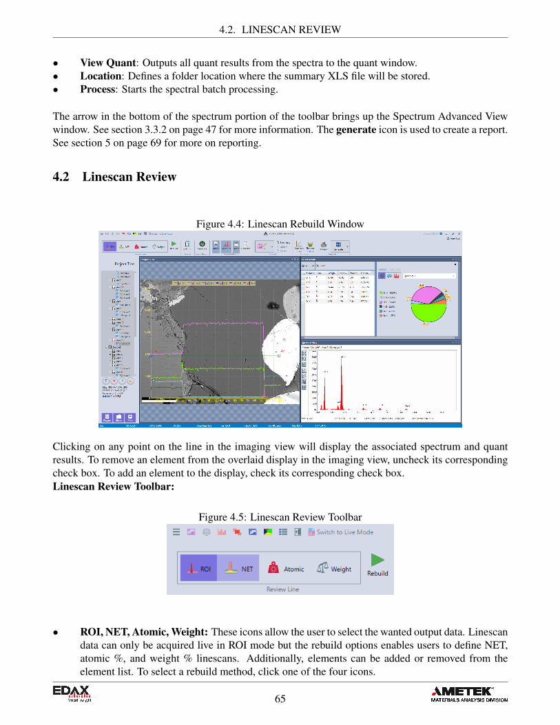
4.2. LINESCAN REVIEW

• View Quant: Outputs all quant results from the spectra to the quant window.• Location: Defines a folder location where the summary XLS file will be stored.• Process: Starts the spectral batch processing.

The arrow in the bottom of the spectrum portion of the toolbar brings up the Spectrum Advanced Viewwindow. See section 3.3.2 on page 47 for more information. The generate icon is used to create a report.See section 5 on page 69 for more on reporting.

4.2 Linescan Review

Figure 4.4: Linescan Rebuild Window

Clicking on any point on the line in the imaging view will display the associated spectrum and quantresults. To remove an element from the overlaid display in the imaging view, uncheck its correspondingcheck box. To add an element to the display, check its corresponding check box.Linescan Review Toolbar:

Figure 4.5: Linescan Review Toolbar

• ROI, NET, Atomic, Weight: These icons allow the user to select the wanted output data. Linescandata can only be acquired live in ROI mode but the rebuild options enables users to define NET,atomic %, and weight % linescans. Additionally, elements can be added or removed from theelement list. To select a rebuild method, click one of the four icons.

65

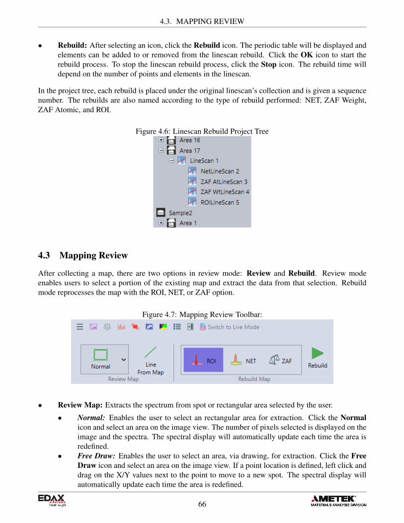
4.3. MAPPING REVIEW

• Rebuild: After selecting an icon, click the Rebuild icon. The periodic table will be displayed andelements can be added to or removed from the linescan rebuild. Click the OK icon to start therebuild process. To stop the linescan rebuild process, click the Stop icon. The rebuild time willdepend on the number of points and elements in the linescan.

In the project tree, each rebuild is placed under the original linescan’s collection and is given a sequencenumber. The rebuilds are also named according to the type of rebuild performed: NET, ZAF Weight,ZAF Atomic, and ROI.

Figure 4.6: Linescan Rebuild Project Tree

4.3 Mapping Review

After collecting a map, there are two options in review mode: Review and Rebuild. Review modeenables users to select a portion of the existing map and extract the data from that selection. Rebuildmode reprocesses the map with the ROI, NET, or ZAF option.

Figure 4.7: Mapping Review Toolbar:

• Review Map: Extracts the spectrum from spot or rectangular area selected by the user.

• Normal: Enables the user to select an rectangular area for extraction. Click the Normalicon and select an area on the image view. The number of pixels selected is displayed on theimage and the spectra. The spectral display will automatically update each time the area isredefined.

• Free Draw: Enables the user to select an area, via drawing, for extraction. Click the FreeDraw icon and select an area on the image view. If a point location is defined, left click anddrag on the X/Y values next to the point to move to a new spot. The spectral display willautomatically update each time the area is redefined.

66

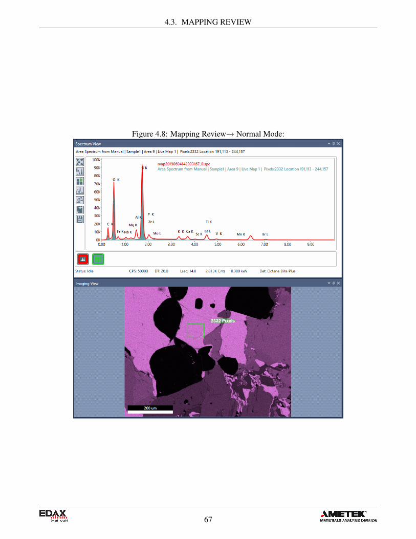
4.3. MAPPING REVIEW

Figure 4.8: Mapping Review→ Normal Mode:

67

4.3. MAPPING REVIEW

• Line from Map: This option extracts a line profile from the collected X-ray map. Click theLine From Map icon and then draw a line on the map to see a profile. The current elementlist will be displayed on the image view. Click OK to the start the linescan generation. Afterthe linescan is created, it will appear on the project tree below the map data with a sequencenumber. Each linescan will also be labeled according to the type of extraction: ROI, NET, orZAF. To build another linescan, use the Back To Map icon to return to the mapping display.

Figure 4.9: Line from Map Project Tree and Back to Map Icon:

• Rebuild Map: Maps can be rebuilt into three types of data: ROI, NET, or ZAF. The ROI mapsdisplay is in scaled raw counts, the NET maps display in background subtracted counts per second,and the ZAF (quant) maps from a scale of 0-100 weight% or atomic%. In the project tree, eachmap rebuild is assigned sequence number named by the type of rebuild. In the ROI and NETmodes, a single output data set will be created, but rebuilding using ZAF mode creates NET, ZAFAtomic %, and ZAF Weight % datasets.

Figure 4.10: Map Rebuild Project Tree:

• Rebuild: Use this icon to start the rebuilding process. The rebuild list of elements willappear on the screen for selection at the start of the process.

68

Chapter 5

Reporting and Printing

5.1 Report Generation: Live Mode

APEX™allows users to easily create reports in Microsoft Word or PowerPoint, while in still live mode.The report icons, in the top right corner of the collection toolbar, enable the user to generate a reportusing pre-existing template or design a template. To use a pre-existing template, select one of the optionsfrom the drop down menu. A preview of the report will be displayed as the mouse is hovered over eachoption.

Figure 5.1: Report Icons: Live Mode, Report Generating

Report Designer

To create a report template for future use, click the Designer icon on the collection toolbar. This willopen a blank template that can be customized.

On the right side of the screen, select a report type from the drop down menu and then select Insert Acrossor Insert Down to specify the layout of the report. Use the Insert Spectrum and Insert Image icons toadd wanted features to the report. Currently the template only supports one spectrum and one image perpage. Extra pages and a company logo can also be added to the template using the corresponding icons.To save the template, enter a file name in the box and click the blue Done icon. This template will nowappear in the Report Template Menu for future use.

Auto Report

Clicking the Auto Report icon will enable Auto Report and change the icon color (shown in Figure 5.5).When Auto Report is enabled, the report engine will generate a report as soon as data collection finishes(orange dots will appear under the Generate icon while the report is loading). New data collection willbe added to the report automatically as long as Auto Report is turned on. Since the report engine worksindependently, data collection and review can continue while the report is being generated.

69

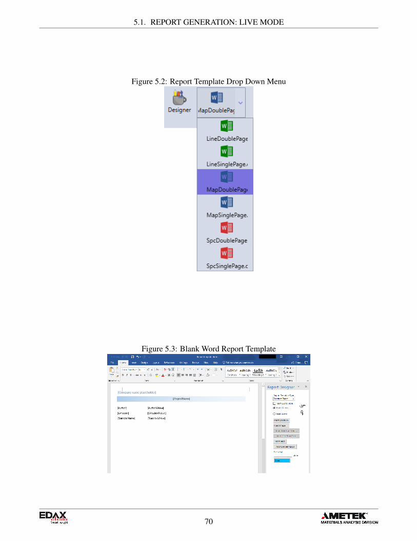
5.1. REPORT GENERATION: LIVE MODE

Figure 5.2: Report Template Drop Down Menu

Figure 5.3: Blank Word Report Template

70

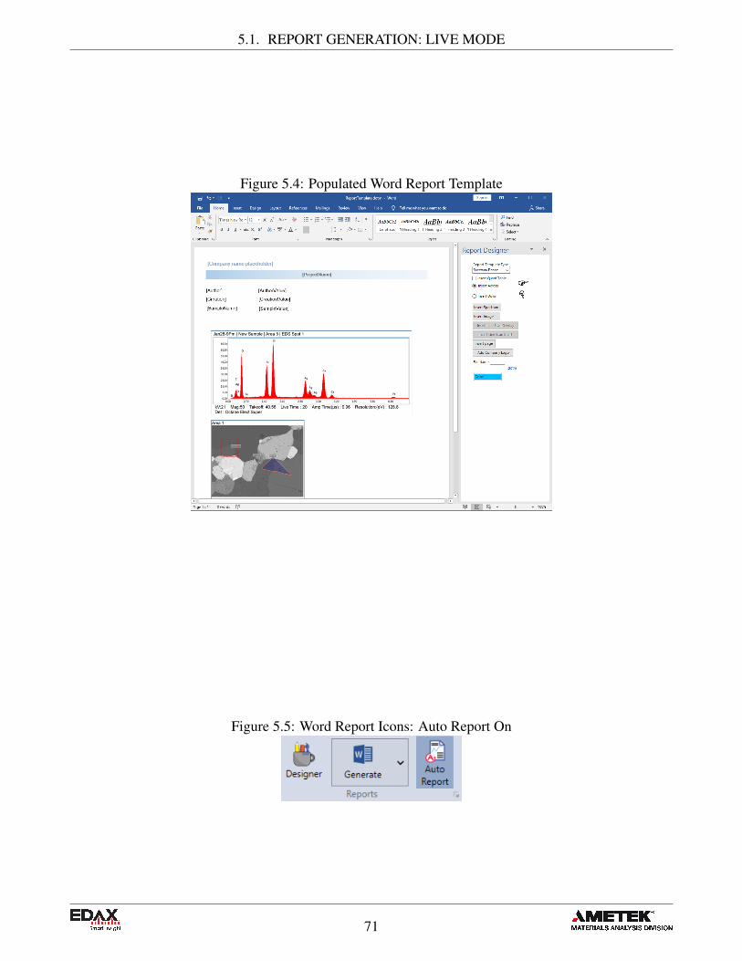
5.1. REPORT GENERATION: LIVE MODE

Figure 5.4: Populated Word Report Template

Figure 5.5: Word Report Icons: Auto Report On

71

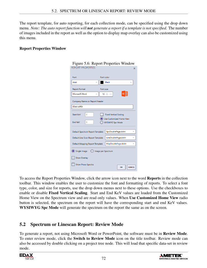
5.2. SPECTRUM OR LINESCAN REPORT: REVIEW MODE

The report template, for auto reporting, for each collection mode, can be specified using the drop downmenu. Note: The auto report function will not generate a report if a template is not specified. The numberof images included in the report as well as the option to display map overlay can also be customized usingthis menu.

Report Properties Window

Figure 5.6: Report Properties Window

To access the Report Properties Window, click the arrow icon next to the word Reports in the collectiontoolbar. This window enables the user to customize the font and formatting of reports. To select a fonttype, color, and size for reports, use the drop down menus next to these options. Use the checkboxes toenable or disable Fixed Vertical Scaling. Start and End KeV values are loaded from the CustomizedHome View on the Spectrum view and are read only values. When Use Customized Home View radiobutton is selected, the spectrum on the report will have the corresponding start and end KeV values.WYSIWYG Spc Mode will generate the spectrum on the report the same as on the screen.

5.2 Spectrum or Linescan Report: Review Mode

To generate a report, not using Microsoft Word or PowerPoint, the software must be in Review Mode.To enter review mode, click the Switch to Review Mode icon on the title toolbar. Review mode canalso be accessed by double clicking on a project tree node. This will load that specific data-set in reviewmode.

72

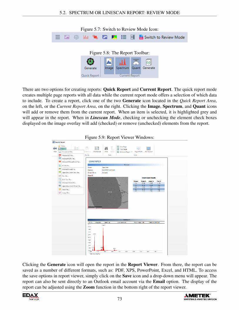
5.2. SPECTRUM OR LINESCAN REPORT: REVIEW MODE

Figure 5.7: Switch to Review Mode Icon:

Figure 5.8: The Report Toolbar:

There are two options for creating reports: Quick Report and Current Report. The quick report modecreates multiple page reports with all data while the current report mode offers a selection of which datato include. To create a report, click one of the two Generate icon located in the Quick Report Area,on the left, or the Current Report Area, on the right. Clicking the Image, Spectrum, and Quant iconswill add or remove them from the current report. When an item is selected, it is highlighted grey andwill appear in the report. When in Linescan Mode, checking or unchecking the element check boxesdisplayed on the image overlay will add (checked) or remove (unchecked) elements from the report.

Figure 5.9: Report Viewer Windows:

Clicking the Generate icon will open the report in the Report Viewer. From there, the report can besaved as a number of different formats, such as: PDF, XPS, PowerPoint, Excel, and HTML. To accessthe save options in report viewer, simply click on the Save icon and a drop-down menu will appear. Thereport can also be sent directly to an Outlook email account via the Email option. The display of thereport can be adjusted using the Zoom function in the bottom right of the report viewer.

73

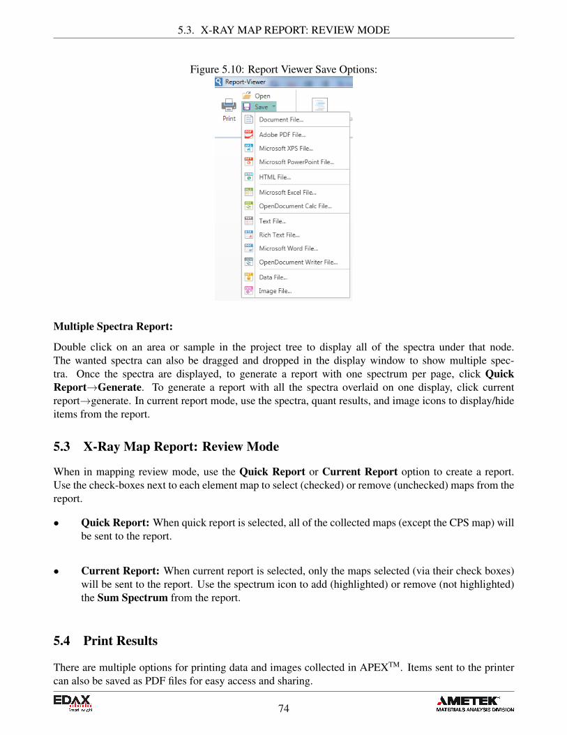
5.3. X-RAY MAP REPORT: REVIEW MODE

Figure 5.10: Report Viewer Save Options:

Multiple Spectra Report:

Double click on an area or sample in the project tree to display all of the spectra under that node.The wanted spectra can also be dragged and dropped in the display window to show multiple spec-tra. Once the spectra are displayed, to generate a report with one spectrum per page, click QuickReport→Generate. To generate a report with all the spectra overlaid on one display, click currentreport→generate. In current report mode, use the spectra, quant results, and image icons to display/hideitems from the report.

5.3 X-Ray Map Report: Review Mode

When in mapping review mode, use the Quick Report or Current Report option to create a report.Use the check-boxes next to each element map to select (checked) or remove (unchecked) maps from thereport.

• Quick Report: When quick report is selected, all of the collected maps (except the CPS map) willbe sent to the report.

• Current Report: When current report is selected, only the maps selected (via their check boxes)will be sent to the report. Use the spectrum icon to add (highlighted) or remove (not highlighted)the Sum Spectrum from the report.

5.4 Print Results

There are multiple options for printing data and images collected in APEXTM. Items sent to the printercan also be saved as PDF files for easy access and sharing.

74

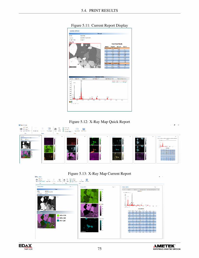
5.4. PRINT RESULTS

Figure 5.11: Current Report Display

Figure 5.12: X-Ray Map Quick Report

Figure 5.13: X-Ray Map Current Report

75

5.4. PRINT RESULTS

• Print Image: To print an image, use the Send to Folder option on the image view. Then, openthe saved image the folder and print the image.

• Print Spectrum: To print a spectrum, use the Send to Folder option on the spectrum view. Then,open the file to print.

• Print Quant: To print quant results, use the Print Icon in the quant menu. Click the icon and thenselect a printing method.

• Print Screen: To print the entire APEXTM screen, use the print icon in the bottom left corner ofthe project tree.

• Print Report: To print a report, generate a report in report viewer. Then, click the Print Icon inthe top left of the screen.

76

Chapter 6

Data Handling and Backup

Note: The contents of this section may be duplicated in other parts of the manual. They are reiteratedhere due to their importance.

6.1 Export and Backup Data

The export, import, and merge functions can be located via the icons in the bottom left of the projecttree.

• Export: Backs up ALL the selected projects.• Import: Temporarily displays data that was exported (usually from some other workstation), but

does not save the actual data on the local computer.• Merge: Imports the data from a different workstation system, and this data becomes part of the

local database. Once data is merged it is permanently on the workstation.

Export Icon:

Clicking the Export button will display the following window. Using the check boxes, select the projectsto be backed up. In the top right-hand corner of the pop-up window, there are three boxes which enablebatch selection of projects.

• First box: Collapse ALL→ All Project nodes are collapsed.• Second box: Check ALL→ All Project nodes are checked (enabled for backup).• Third box: Un-Check ALL → All Project nodes are un-checked. As a default, this is how the

window is first displayed.

Next, click the OK button and choose a destination folder for data backup and click Select Folder. Ifthe selected backup folder already exists the message below will be displayed. Click Yes to overwriteand start the backup process. While the backup is running, a progress window will be displayed on thescreen. Click the Stop button to stop the backup process.Each project is saved as a Zip file and each sub folder is date and time stamped; i.e. Backup on Tue04.11.2017 At 15.05 PM. The database entries are in the *.BAK file, the raw APEX data is in the *.ZIPfile, and the a name listing of all the backed up files is in the *.XML file.

77

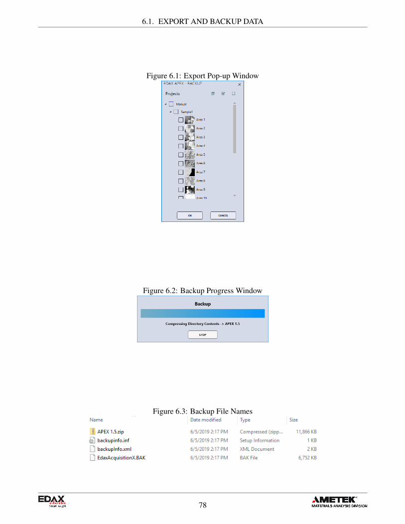
6.1. EXPORT AND BACKUP DATA

Figure 6.1: Export Pop-up Window

Figure 6.2: Backup Progress Window

Figure 6.3: Backup File Names

78

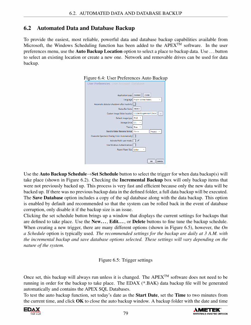
6.2. AUTOMATED DATA AND DATABASE BACKUP

6.2 Automated Data and Database Backup

To provide the easiest, most reliable, powerful data and database backup capabilities available fromMicrosoft, the Windows Scheduling function has been added to the APEXTM software. In the userpreferences menu, use the Auto Backup Location option to select a place to backup data. Use . . . buttonto select an existing location or create a new one. Network and removable drives can be used for databackup.

Figure 6.4: User Preferences Auto Backup

Use the Auto Backup Schedule→Set Schedule button to select the trigger for when data backup(s) willtake place (shown in Figure 6.2). Checking the Incremental Backup box will only backup items thatwere not previously backed up. This process is very fast and efficient because only the new data will bebacked up. If there was no previous backup data in the defined folder, a full data backup will be executed.The Save Database option includes a copy of the sql database along with the data backup. This optionis enabled by default and recommended so that the system can be rolled back in the event of databasecorruption, only disable it if the backup size is an issue.Clicking the set schedule button brings up a window that displays the current settings for backups thatare defined to take place. Use the New. . . , Edit. . . , or Delete buttons to fine tune the backup schedule.When creating a new trigger, there are many different options (shown in Figure 6.5), however, the Ona Schedule option is typically used. The recommended settings for the backup are daily at 3 A.M. withthe incremental backup and save database options selected. These settings will vary depending on thenature of the system.

Figure 6.5: Trigger settings

Once set, this backup will always run unless it is changed. The APEXTM software does not need to berunning in order for the backup to take place. The EDAX (*.BAK) data backup file will be generatedautomatically and contains the APEX SQL Databases.To test the auto backup function, set today’s date as the Start Date, set the Time to two minutes fromthe current time, and click OK to close the auto backup window. A backup folder with the date and time

79

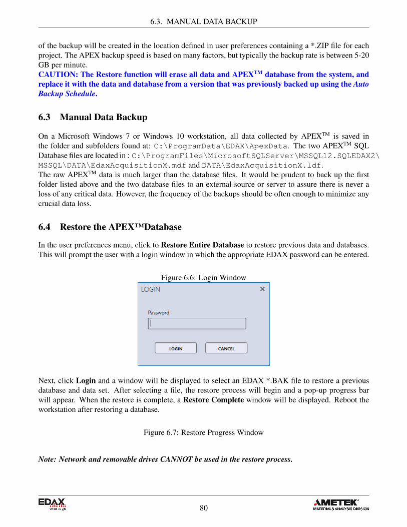
6.3. MANUAL DATA BACKUP

of the backup will be created in the location defined in user preferences containing a *.ZIP file for eachproject. The APEX backup speed is based on many factors, but typically the backup rate is between 5-20GB per minute.CAUTION: The Restore function will erase all data and APEXTM database from the system, andreplace it with the data and database from a version that was previously backed up using the AutoBackup Schedule.

6.3 Manual Data Backup

On a Microsoft Windows 7 or Windows 10 workstation, all data collected by APEXTM is saved inthe folder and subfolders found at: C:\ProgramData\EDAX\ApexData. The two APEXTM SQLDatabase files are located in : C:\ProgramFiles\MicrosoftSQLServer\MSSQL12.SQLEDAX2\MSSQL\DATA\EdaxAcquisitionX.mdf and DATA\EdaxAcquisitionX.ldf.The raw APEXTM data is much larger than the database files. It would be prudent to back up the firstfolder listed above and the two database files to an external source or server to assure there is never aloss of any critical data. However, the frequency of the backups should be often enough to minimize anycrucial data loss.

6.4 Restore the APEX™Database

In the user preferences menu, click to Restore Entire Database to restore previous data and databases.This will prompt the user with a login window in which the appropriate EDAX password can be entered.

Figure 6.6: Login Window

Next, click Login and a window will be displayed to select an EDAX *.BAK file to restore a previousdatabase and data set. After selecting a file, the restore process will begin and a pop-up progress barwill appear. When the restore is complete, a Restore Complete window will be displayed. Reboot theworkstation after restoring a database.

Figure 6.7: Restore Progress Window

Note: Network and removable drives CANNOT be used in the restore process.

80

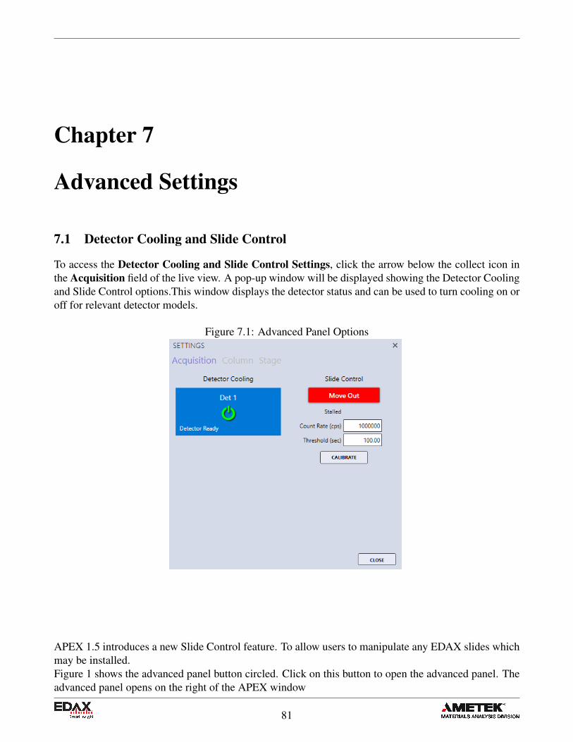
Chapter 7

Advanced Settings

7.1 Detector Cooling and Slide Control

To access the Detector Cooling and Slide Control Settings, click the arrow below the collect icon inthe Acquisition field of the live view. A pop-up window will be displayed showing the Detector Coolingand Slide Control options.This window displays the detector status and can be used to turn cooling on oroff for relevant detector models.

Figure 7.1: Advanced Panel Options

APEX 1.5 introduces a new Slide Control feature. To allow users to manipulate any EDAX slides whichmay be installed.Figure 1 shows the advanced panel button circled. Click on this button to open the advanced panel. Theadvanced panel opens on the right of the APEX window

81

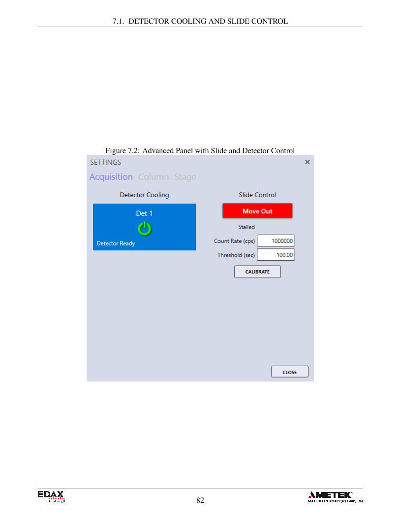
7.1. DETECTOR COOLING AND SLIDE CONTROL

Figure 7.2: Advanced Panel with Slide and Detector Control

82

7.2. MICROSCOPE COLUMN AND STAGE CONTROL

Moving the Slide

Before moving the slide in make sure the detector is ready. To move the slide click the “MOVE IN”button. Once the slide is in the button label changes to “MOVE OUT” and the color changes to green.The slide status will state Slide In. To move the slide out click the “MOVE OUT” button.

Count Rate and Threshold

The Count Rate determines the maximum counts the counts the slide will tolerate while in the IN posi-tion. The Threshold is the time limit that the slide will tolerate the maximum count rate before movingout. Figure 4 shows the slide in an “Auto Retracted” state after passing the maximum count rate andthreshold.

Calibrating the Slide

To calibrate the slide click the Calibrate button. The button will be disabled until the calibration iscomplete. Slide calibration finds the slides analyze and retract positions.

7.2 Microscope Column and Stage Control

The EDAX Column and Stage control options are only available for certain microscopes and must beinstalled and configured. To access the Column and Stage Control Settings, click the arrow belowthe collect icon in the Acquisition field of the live view. A pop-up window will be displayed showingthe Column/ Stage control options. This window is a floating window which enables users to makeadjustments while collecting an image and see those changes immediately.

Figure 7.3: Acquisition field

To switch on or off the Microscope High Tension, slide the HT On/Off slider control. To turn off thehigh tension after a lengthy analysis, use the Auto Beam-OFF check box before starting the analysis.This function is typically used for X-ray maps, linescans, or multipoint spectral analysis.Click Stage to show the stage control options. Use the X and Y boxes to specify a stage location. ClickSet XY to move the stage to that location. Click Read Positions to update the X and Y values after thestage has been moved via the controls on the microscope.Note: If the stage and column control options are not available, this window can still be used to setthe magnification and KV to match the SEM conditions prior to the analysis.

7.3 Spectral Calibration

It is recommended that the spectral calibration is verified periodically. When the spectrum deconvolutiondoes not match the collection spectra, the software should be calibrated. Typically this is done using anAluminum and Copper specimen. Load this type of sample into the SEM and adjust the beam current for

83

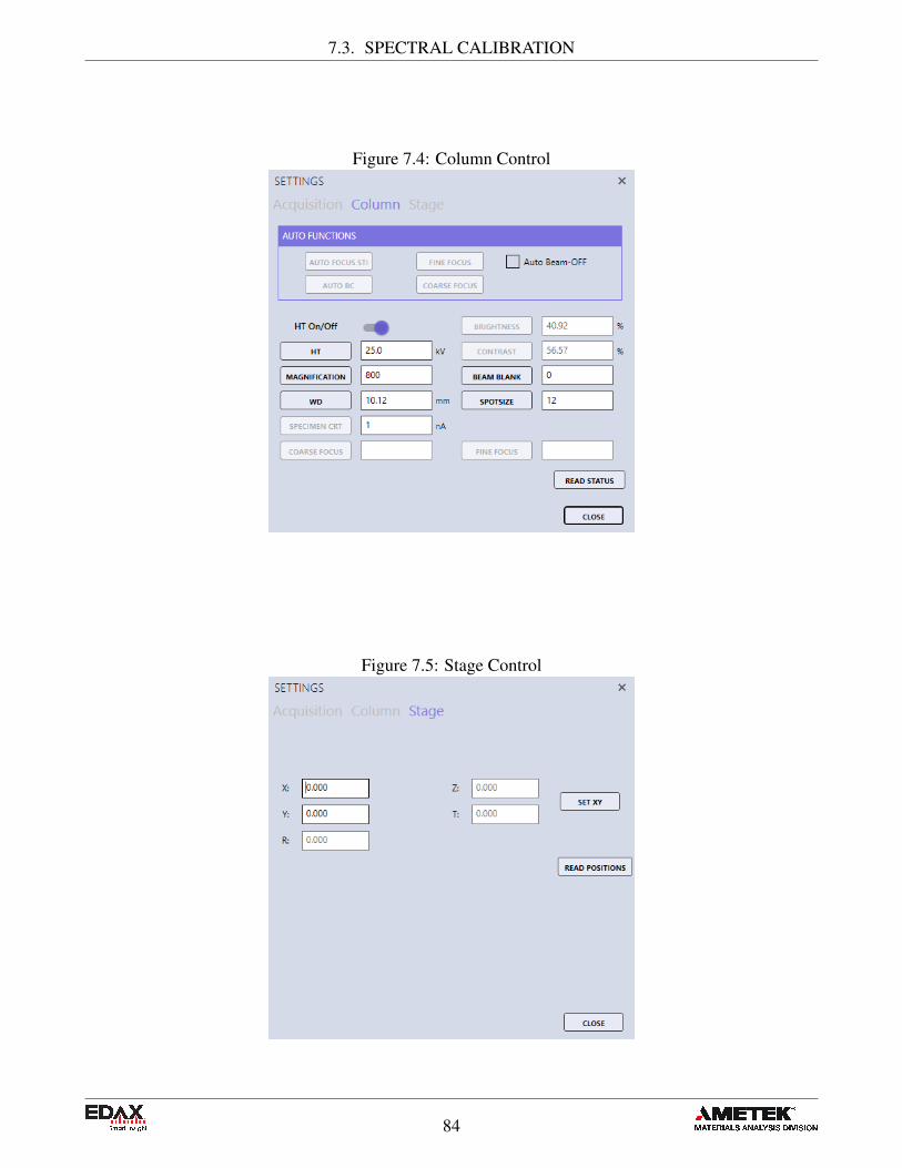
7.3. SPECTRAL CALIBRATION

Figure 7.4: Column Control

Figure 7.5: Stage Control

84

7.3. SPECTRAL CALIBRATION

roughly 15,000 CPS. The high tension should be set to above 25 kV and the SEM field of view shouldbe adjusted so the Al K and Cu K peaks are of roughly equal height in the spectrum view. Right click onthe spectrum view window and select Calibration Tools from the options menu. Then click Calibrate.

Figure 7.6: Calibration Menu

APEX will immediately collect a spectrum for a short period of time. If an Aluminum and Copperspecimen is being used, the target energies are preset in the software and the calibration can be startedusing the Calibrate button. If a different specimen is being used for the calibration, the two targetenergies must be entered manually, in keV, in the Peak 1 and Peak 2 boxes before clicking the Calibratebutton. It is recommended the energies be large, non-overlapping peaks several keV apart in energy andabove 1 keV.

Figure 7.7: Calibration Collection and Complete Windows

Clicking the Calibrate button will start the spectrum acquisition and when the two peak energies arewithin specification, the calibration is complete. During the calibration, the window title will displaythat calibration is in progress. The window can be moved around by clicking on the title and dragging.The Delta values are the difference (in keV) between the target and measured peak energies. Click

85

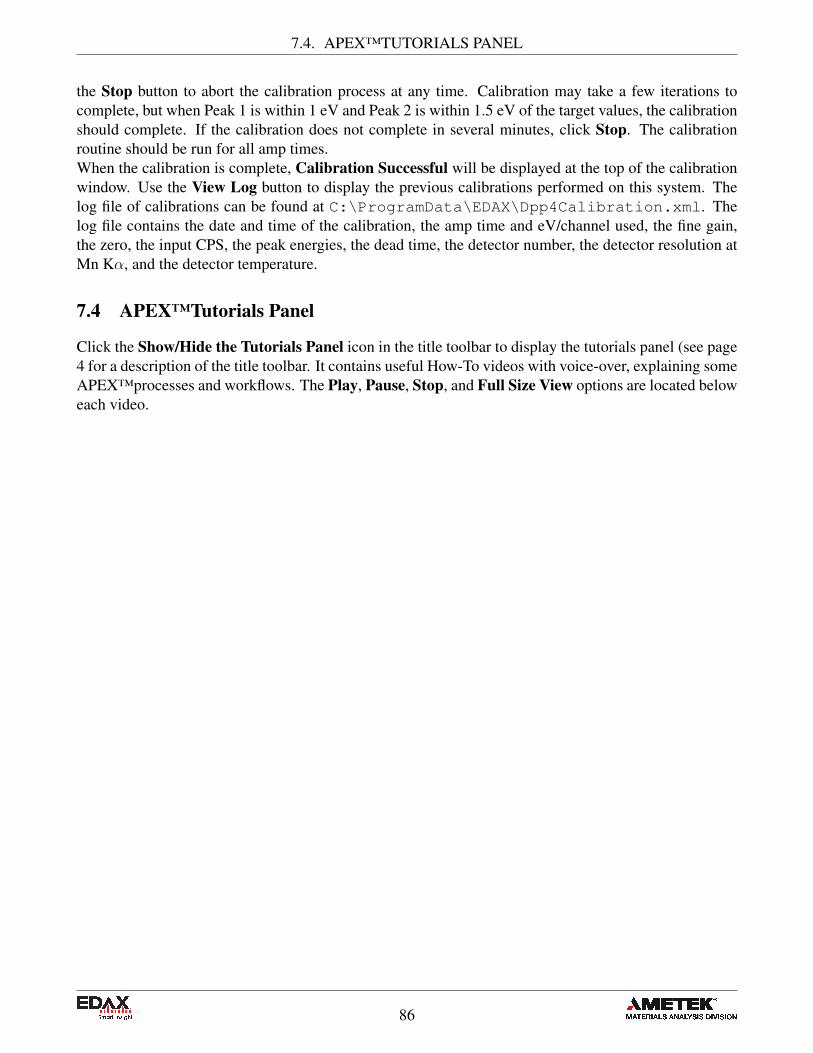
7.4. APEX™TUTORIALS PANEL

the Stop button to abort the calibration process at any time. Calibration may take a few iterations tocomplete, but when Peak 1 is within 1 eV and Peak 2 is within 1.5 eV of the target values, the calibrationshould complete. If the calibration does not complete in several minutes, click Stop. The calibrationroutine should be run for all amp times.When the calibration is complete, Calibration Successful will be displayed at the top of the calibrationwindow. Use the View Log button to display the previous calibrations performed on this system. Thelog file of calibrations can be found at C:\ProgramData\EDAX\Dpp4Calibration.xml. Thelog file contains the date and time of the calibration, the amp time and eV/channel used, the fine gain,the zero, the input CPS, the peak energies, the dead time, the detector number, the detector resolution atMn Kα, and the detector temperature.

7.4 APEX™Tutorials Panel

Click the Show/Hide the Tutorials Panel icon in the title toolbar to display the tutorials panel (see page4 for a description of the title toolbar. It contains useful How-To videos with voice-over, explaining someAPEX™processes and workflows. The Play, Pause, Stop, and Full Size View options are located beloweach video.

86

apex user manual - research

Documents