Appendix: 3D Shape Generation and Completion through Point-Voxel Diffusion

A. Additional Generation MetricsWe present additional generation metrics in Table 1, fol-

lowing PointFlow [9]. We report coverage (COV), whichmeasures the fraction of point clouds in the reference setthat are matched to at least one point cloud in the generatedset. We further report minimum matching distance (MMD),which measures for each point cloud in a reference set, thedistance to its nearest neighbor in the generated set. Notethat these generation metrics can vary depending on im-plementation and do not necessarily correlate to generationquality, as discussed in [9].

Table 2 includes generation results on Airplane, Chair,Car compared with the voxel-diffusion model, Vox-Diff,as described in the main paper, evaluated using the 1-NNmetric. By generating less noisy point clouds, PVD signifi-cantly outperforms Vox-Diff.

B. Point Cloud Generation VisualizationWe additionally visualize some generation results for

Airplane, Car, and Chair in terms of the generation pro-cess and the final generated shapes from all angles in Fig-ures 3, 4, 5. 6, 7, 8, 9, and 10.

C. Derivation of the Variational Lower Bound

Eq(x0)[log pθ(x0)] = Eq(x0)

[log

∫pθ(x0, ...,xT ) dx1:T

]≥ Eq(x0)

[ ∫q(x1, ...,xT |x0)

logpθ(x0, ...,xT )

q(x1, ...,xT |x0)dx1:T

]= Eq(x0:T )

[log

pθ(x0, ...,xT )

q(x1, ...,xT |x0)

],

where the inequality is by Jensen’s inequality.

D. Properties of the Diffusion Model{β0, ..., βT } is a sequence of increasing parameters;

αt = 1 − βt and αt =∏t

s=1 αs. Two following proper-ties are crucial to deriving the final L2 loss.

Property 1. Tractable marginal of the forward process:

q(xt|x0) =

∫q(x1:t|x0) dx1:(t−1)

= N (√

αtx0, (1− αt)I).

This property is proved in the Appendix of [4] and providesconvenient closed-form evaluation of xt knowing x0:

xt =√αtx0 +

√1− αtϵ, (1)

where ϵ ∼ N (0, I).Property 2. Tractable posterior of the forward process.

We first note the Bayes’ rule that connects the posterior withthe forward process,

q(xt−1|xt,x0) =q(xt|xt−1,x0)q(xt−1|x0)

q(xt|x0).

Since the three probabilities on the right are Gaussian, theposterior is also Gaussian, given by

q(xt−1|xt,x0) =

N (

√αt−1βt

1− αtx0 +

√αt(1− αt−1)

1− αtxt,

(1− αt−1)

1− αtβtI).

(2)

E. Derivation of L2 LossWe need to match generative transition pθ(xt−1|xt)

with ground-truth posterior q(xt−1|xt,x0), both of whichare Gaussian with a pre-determined variance scheduleβ1, ..., βT . Therefore, maximum likelihood learning is re-duced to simple L2 loss of the form with two cases:

Lt =

∥∥∥∥√αt−1βt

1−αtx0 +

√αt(1−αt−1)

1−αtxt − µθ(xt, t)

∥∥∥∥2 , t > 1

∥x0 − µθ(xt, t)∥2 , t = 1

where αt = 1−βt and αt =∏t

s=1 αs. The supervision tar-get of case t > 1 comes from Eqn. 2. We can Further reducethe case when t > 1 by substituting x0 as an expression ofxt using Eqn. 1 and arrive at

Lt =

∥∥∥ 1√

αt

(xt − βt√

1−αtϵ)− µθ(xt, t)

∥∥∥2 , t > 1

∥x0 − µθ(xt, t)∥2 , t = 1

where ϵ ∼ N (0, I).Note that when t = 1, α1 = α1 so that the supervision

target of the first case above evaluated at t = 1 becomes:

1√α1

(x1 −

βt√1− α1

ϵ

)=

1√α1

(x1 −

√1− α1ϵ

)= x0,

(3)where the last equality is by rewriting Eqn. 1. Therefore, infact, the two cases are equivalent.

The final L2 loss is

Lt =

∥∥∥∥ 1√αt

(xt −

βt√1− αt

ϵ

)− µθ(xt, t)

∥∥∥∥2 .

Model

Airplane Chair Car

MMD↓ COV↑ (%) MMD↓ COV↑ (%) MMD↓ COV↑ (%)

CD EMD CD EMD CD EMD CD EMD CD EMD CD EMD

r-GAN [1] 0.4471 2.309 30.12 14.32 5.151 8.312 24.27 15.13 1.446 2.133 19.03 6.539l-GAN (CD) [1] 0.3398 0.5832 38.52 21.23 2.589 2.007 41.99 29.31 1.532 1.226 38.92 23.58l-GAN (EMD) [1] 0.3967 0.4165 38.27 38.52 2.811 1.619 38.07 44.86 1.408 0.8987 37.78 45.17PointFlow [9] 0.2243 0.3901 47.90 46.41 2.409 1.595 42.90 50.00 0.9010 0.8071 46.88 50.00SoftFlow [5] 0.2309 0.3745 46.91 47.90 2.528 1.682 41.39 47.43 1.187 0.8594 42.90 44.60DPF-Net [6] 0.2642 0.4086 46.17 48.89 2.536 1.632 44.71 48.79 1.129 0.8529 45.74 49.43Shape-GF [2] 2.703 0.6592 40.74 40.49 2.889 1.702 46.67 48.03 9.232 0.7558 49.43 50.28Vox-Diff 1.322 0.5610 11.82 25.43 5.840 2.930 17.52 21.75 5.646 1.551 6.530 22.15PVD (Ours) 0.2243 0.3803 48.88 52.09 2.622 1.556 49.84 50.60 1.077 0.7938 41.19 50.56

Table 1: Additional generation metrics, following PointFlow [9].

Airplane Chair Car

CD EMD CD EMD CD EMD

Vox-Diff 99.75 98.13 97.12 96.74 99.56 96.83PVD (ours) 73.82 64.81 56.26 53.32 54.55 53.83

Table 2: Generation results on Airplane, Chair, Car compared withthe voxel-diffusion model, Vox-Diff, as described in the main pa-per, evaluated using the 1-NN metric. By generating less noisypoint clouds, PVD significantly outperforms Vox-Diff.

Since xt is known when x0 is known, we can redefine themodel output as ϵθ(xt, t). Instead of directly predictingµθ(xt, t), we instead predict a noise value ϵθ(xt, t), where

µθ(xt, t) =1

√αt

(xt −

βt√1− αt

ϵθ(xt, t)

). (4)

Substituting in µθ(xt, t) into the loss, we can arrive atthe final loss

∥ϵ− ϵθ(xt, t)∥2 , ϵ ∼ N (0, I). (5)

F. Point Cloud Generation ProcessSince the transition mean µθ(xt, t) of pθ(xt−1|xt) is cal-

culated by Eqn. 4, the generative process is performed byprogressively sampling from pθ(xt−1|xt) as t = T, ..., 1:

xt−1 =1

√αt

(xt −

1− αt√1− αt

ϵθ(xt, t)

)+√βtz, (6)

where z ∼ N (0, I). This approach is also similar toLangevin dynamics [3, 8] used in energy-based models,since it similarly adds scaled noise outputs from the modelto current samples. Specifically, Langevin dynamics is inthe following form:

xt+1 = xt + s∂

∂xlog pθ(x) +

√2sz, (7)

where s denotes step size, pθ(x) denotes the model distri-bution, and z ∼ N (0, I). Both processes are Markovian,shifting the previous output by a model-dependent term anda noise term. The scaled model output of our model canalso be seen as an approximation of gradients of an energyfunction.

G. Controlled Completion

We show that our model can control the shape comple-tion process in Figure 1. Given a pretrained completionmodel, our formulation also enables control over comple-tion results through latent interpolation. The figure belowshows one such case: we may have used the left depth mapto obtain a completed shape. But it comes with an unwantedfeature (cavity at the chair’s back). We can refine the resultby feeding another depth map (shown on the right), with abetter view of the back. To retain features from both partialshapes, we can interpolate by (1 − λ)xT + λyT in the la-tent space at time T , where the latent features are obtainedby xT =

√αT x0 +

√1− αT ϵ (see Eqn. 1). Interpolation

presents diverse choices and users can actively control howmuch features are shared by varying λ.

Figure 1: Controlled completion process.

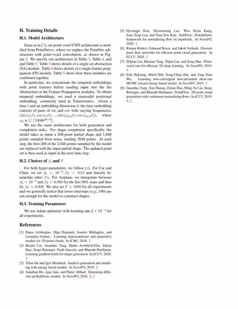
H. Training DetailsH.1. Model Architecture

Same as in [7], our point-voxel CNN architecture is mod-ified from PointNet++, where we replace the PointNet sub-structure with point-voxel convolution, as shown in Fig-ure 2. We specify our architecture in Table 3, Table 4, andand Table 5. Table 3 shows details of a single set abstraction(SA) module. Table 4 shows details of a single feature prop-agation (FP) module. Table 5 shows how these modules arecombined together.

In particular, we concatenate the temporal embeddingswith point features before sending input into the SetAbstraction or the Feature Propagation modules. To obtaintemporal embeddings, we used a sinusoidal positionalembedding, commonly used in Transformers. Given atime t and an embedding dimension d, the time embeddingconsists of pairs of sin and cos with varying frequencies,(sin (ω1t), cos (ω1t), ..., sin (ωd/2t), cos (ωd/2t)), whereωk is 1/

(100002k/d

).

We use the same architecture for both generation andcompletion tasks. For shape completion specifically, themodel takes as input a 200-point partial shape and 1,848points sampled from noise, totaling 2048 points. At eachstep, the first 200 of the 2,048 points sampled by the modelare replaced with the input partial shape. The updated pointset is then used as input in the next time step.

H.2. Choices of βt and T

For both hyper-parameters, we follow [4]. For Car andChair, we set β0 = 10−4, βT = 0.01 and linearly in-terpolate other β’s. For Airplane, we interpolate betweenβ0 = 10−5 and βT = 0.008 for the first 90% steps and thenfix βT = 0.008. We also set T = 1000 for all experimentsand we generally notice that lower timesteps (e.g., 100) arenot enough for the model to construct shapes.

H.3. Training Parameters

We use Adam optimizer with learning rate 2× 10−4 forall experiments.

References[1] Panos Achlioptas, Olga Diamanti, Ioannis Mitliagkas, and

Leonidas Guibas. Learning representations and generativemodels for 3D point clouds. In ICML, 2018. 2

[2] Ruojin Cai, Guandao Yang, Hadar Averbuch-Elor, ZekunHao, Serge Belongie, Noah Snavely, and Bharath Hariharan.Learning gradient fields for shape generation. In ECCV, 2020.2

[3] Yilun Du and Igor Mordatch. Implicit generation and model-ing with energy based models. In NeurIPS, 2019. 2

[4] Jonathan Ho, Ajay Jain, and Pieter Abbeel. Denoising diffu-sion probabilistic models. In NeurIPS, 2020. 1, 3

[5] Hyeongju Kim, Hyeonseung Lee, Woo Hyun Kang,Joun Yeop Lee, and Nam Soo Kim. SoftFlow: Probabilisticframework for normalizing flow on manifolds. In NeurIPS,2020. 2

[6] Roman Klokov, Edmond Boyer, and Jakob Verbeek. Discretepoint flow networks for efficient point cloud generation. InECCV, 2020. 2

[7] Zhijian Liu, Haotian Tang, Yujun Lin, and Song Han. Point-voxel cnn for efficient 3D deep learning. In NeurIPS, 2019.3

[8] Erik Nijkamp, Mitch Hill, Song-Chun Zhu, and Ying NianWu. Learning non-convergent non-persistent short-runMCMC toward energy-based model. In NeurIPS, 2019. 2

[9] Guandao Yang, Xun Huang, Zekun Hao, Ming-Yu Liu, SergeBelongie, and Bharath Hariharan. PointFlow: 3D point cloudgeneration with continuous normalizing flows. In ICCV, 2019.1, 2

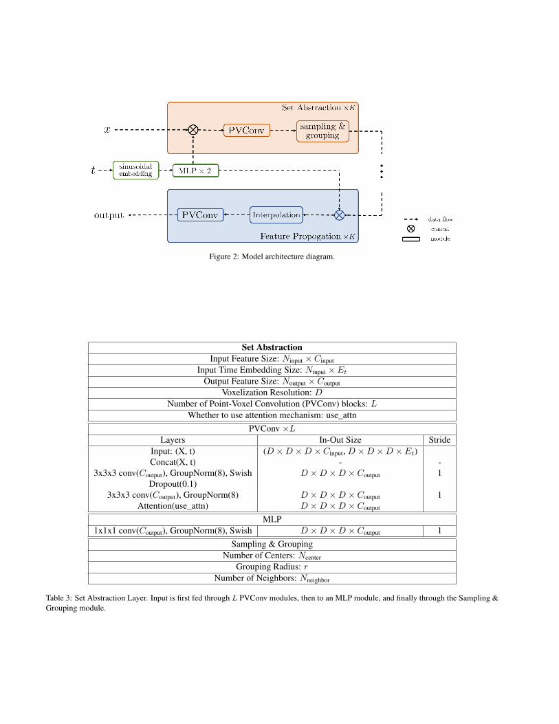
Figure 2: Model architecture diagram.

Set AbstractionInput Feature Size: Ninput × Cinput

Input Time Embedding Size: Ninput × Et

Output Feature Size: Noutput × Coutput

Voxelization Resolution: DNumber of Point-Voxel Convolution (PVConv) blocks: L

Whether to use attention mechanism: use_attnPVConv ×L

Layers In-Out Size StrideInput: (X, t) (D ×D ×D × Cinput, D ×D ×D × Et)Concat(X, t) - -

3x3x3 conv(Coutput), GroupNorm(8), Swish D ×D ×D × Coutput 1Dropout(0.1)

3x3x3 conv(Coutput), GroupNorm(8) D ×D ×D × Coutput 1Attention(use_attn) D ×D ×D × Coutput

MLP1x1x1 conv(Coutput), GroupNorm(8), Swish D ×D ×D × Coutput 1

Sampling & GroupingNumber of Centers: Ncenter

Grouping Radius: rNumber of Neighbors: Nneighbor

Table 3: Set Abstraction Layer. Input is first fed through L PVConv modules, then to an MLP module, and finally through the Sampling &Grouping module.

Feature PropagationInput Feature Size: Ninput × Cinput

Output Feature Size: Noutput × Coutput

Voxelization Resolution: DNumber of Point-Voxel Convolution (PVConv) blocks: L

Whether to use attention mechanism: use_attnInterpolationPVConv ×L

Layers In-Out Size StrideInput: X D ×D ×D × Cinput

3x3x3 conv(Coutput), GroupNorm(8), Swish D ×D ×D × Coutput 1Dropout(0.1)

3x3x3 conv(Coutput), GroupNorm(8) D ×D ×D × Coutput 1Attention(use_attn) D ×D ×D × Coutput

MLP3x3x3 conv(Coutput), GroupNorm(8), Swish D ×D ×D × Coutput 1

Table 4: Feature Propagation Layer. Input is fed through Interpolation module, L PVConv modules, and an MLP module.

Input Feature Size: 2048× 3Input Time Embedding Size: 64Output Feature Size: 2048× 3

Time EmbeddingSinusoidal Embedding dim = 64

MLP(64, 64)LeakyRelU(0.1)

MLP(64, 64)SA 1 SA 2 SA 3 SA 4

L 2 3 3 0Cinput 3 32 64 -Et 64 64 64 -

Coutput 32 64 128 -D 32 16 8 -

use_attn False True False -Ncenter 1024 256 64 16

r 0.1 0.2 0.4 0.8Nneighbor 32 32 32 32

FP 1 FP 2 FP 3 FP 4L 3 3 2 2

Cinput 128 256 256 128Coutput 256 256 128 64D 8 8 16 32

use_attn False True False FalseMLP(64,3)

Table 5: Entire point-voxel CNN architecture. Input point clouds and time steps are sequentially passed through SA 1-4, FP 1-4, andan MLP to obtain output of the same dimension. At the start of each SA and FP module, time embedding and point features are firstconcatenated.

Figure 3: Airplane generation process.

Figure 4: Airplane results from all angles.

Figure 5: Car generation process.

Figure 6: Car results from all angles.

Figure 7: Chair generation process.

Figure 8: Chair results from all angles.

Figure 9: Chair generation process.

Figure 10: Chair results from all angles.