61

APPENDIX A – Methods for the 1997 Sampling, including Aerial Survey Standard Operating Procedures

Methods for the 1997 Sampling, including Aerial Survey Standard Operating Procedures The Aerial Survey Standard Operating Procedures (SOP) is included here for its detail and because it was not included in Irvine (1998). Following that is a section of Methods from Irvine (1998), which concentrates on the coarse-grained (CG) and fine-grained (FG) sampling and just briefly refers to the aerial surveys. In the Methods section, note that the table and figure numbers refer to ones in the current report, unless indicated as being found only in the 1998 report.

62

September 30, 1997

Standard Operating Procedures for

AERIAL SURVEYS for

Development of Coastal Monitoring Protocols and Process-Based Studies to Address Landscape-Scale Variation in Coastal Communities of Glacier Bay National Park and Preserve (GLBA),

Katmai National Park and Preserve (KATM), and Wrangell-St. Elias National Park and Preserve (WRST)

Purpose

The purpose of monitoring programs is to detect change in populations or communities through time. If populations and communities are stable, then only an inventory of the populations or communities would be required. An inventory over large areas requires sampling to make inferences regarding populations over the area of interest. Glacier Bay proper encompasses over one thousand kilometers of coastline. As this is far too large to be thoroughly sampled, aerial surveys were carried out in order to provide a preliminary assessment of substrate and biota compositions and thus aid in selection of the sites to be sampled as part of the coarse and fine-grained sampling levels of the project. The aerial surveys provided estimates of the relative abundance of different substrate types (bedrock, cobble/boulder, pebble/gravel, sand/silt/mud, coarse sand) within segments as well as biota (Fucus, mussels, barnacles). These standard operating procedures were used in 1997 when performing aerial surveys for the coastal monitoring protocol development study.

Site Selection

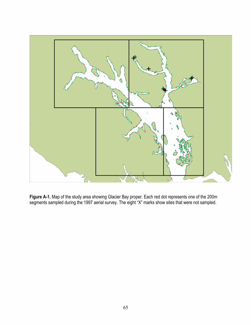
Within Glacier Bay National Park and Preserve the coastline of Glacier Bay proper (the inner part of Glacier Bay NP&P, from Pt. Carolus and Pt. Gustavus northward) was divided into 200 m segments using ArcInfo software and a digitized coastline (CD-ROM; Geiselman, J. et al. 1997). This resulted in the identification of 5,545 segments representing a coastline of 1,109 km. Based on our assessment that we could aerially survey 250 segments during one minus tide cycle, a random number was used to identify a starting segment, and every twenty-third segment was then systematically chosen, resulting in 250 segments. Ultimately, 241 segments were surveyed by fixed-wing airplane. Segments 173, 174, and 175 were not surveyed because they were part of a stream bank rather than intertidal areas. Segment 192 also was not an intertidal site and was not surveyed. Segments 185 and 186 were not surveyed because they were on a large mud delta criss-crossed by streams and still snow-covered. The areas matching the coordinates for segments 17 and 205 did not even vaguely resemble the segment maps from ArcInfo, thus they were not surveyed. This area of the Park has been undergoing rapid sedimentation and is now quite different than when the last charts were created. Segment 190 was not sampled because it was still covered in ice and snow. See figure A-1 for a map of the study area and segments.

63

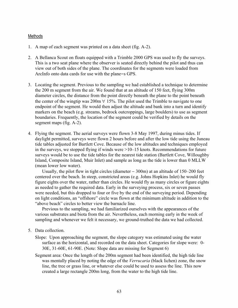
Methods

1. A map of each segment was printed on a data sheet (fig. A-2). 2. A Bellanca Scout on floats equipped with a Trimble 2000 GPS was used to fly the surveys.

This is a two seat plane where the observer is seated directly behind the pilot and thus can view out of both sides of the plane. The coordinates for the segments were loaded from ArcInfo onto data cards for use with the plane=s GPS.

3. Locating the segment. Previous to the sampling we had established a technique to determine

the 200 m segment from the air. We found that at an altitude of 150 feet, flying 300m diameter circles, the distance from the point directly beneath the plane to the point beneath the center of the wingtip was 200m ∀ 15%. The pilot used the Trimble to navigate to one endpoint of the segment. He would then adjust the altitude and bank into a turn and identify markers on the beach (e.g. streams, bedrock outcroppings, large boulders) to use as segment boundaries. Frequently, the location of the segment could be verified by details on the segment maps (fig. A-2).

4. Flying the segment. The aerial surveys were flown 3-8 May 1997, during minus tides. If

daylight permitted, surveys were flown 2 hours before and after the low tide using the Juneau tide tables adjusted for Bartlett Cove. Because of the low altitudes and techniques employed in the surveys, we stopped flying if winds were >10–15 knots. Recommendations for future surveys would be to use the tide tables for the nearest tide station (Bartlett Cove, Willoughby Island, Composite Island, Muir Inlet) and sample as long as the tide is lower than 0 MLLW (mean lower low water).

Usually, the pilot flew in tight circles (diameter − 300m) at an altitude of 150–200 feet centered over the beach. In steep, constricted areas (e.g. Johns Hopkins Inlet) he would fly figure eights over the water, rather than circles. He would fly as many circles or figure eights as needed to gather the required data. Early in the surveying process, six or seven passes were needed, but this dropped to four or five by the end of the surveying period. Depending on light conditions, an “offshore” circle was flown at the minimum altitude in addition to the “above beach” circles to better view the barnacle line.

Previous to the sampling, we had familiarized ourselves with the appearances of the various substrates and biota from the air. Nevertheless, each morning early in the week of sampling and whenever we felt it necessary, we ground-truthed the data we had collected.

5. Data collection.

Slope: Upon approaching the segment, the slope category was estimated using the water surface as the horizontal, and recorded on the data sheet. Categories for slope were: 0-30Ε, 31-60Ε, 61-90Ε. (Note: Slope data are missing for Segment 6)

Segment area: Once the length of the 200m segment had been identified, the high tide line was mentally placed by noting the edge of the Verrucaria (black lichen) zone, the snow line, the tree or grass line, or whatever else could be used to assess the line. This now created a large rectangle 200m long, from the water to the high tide line.

64

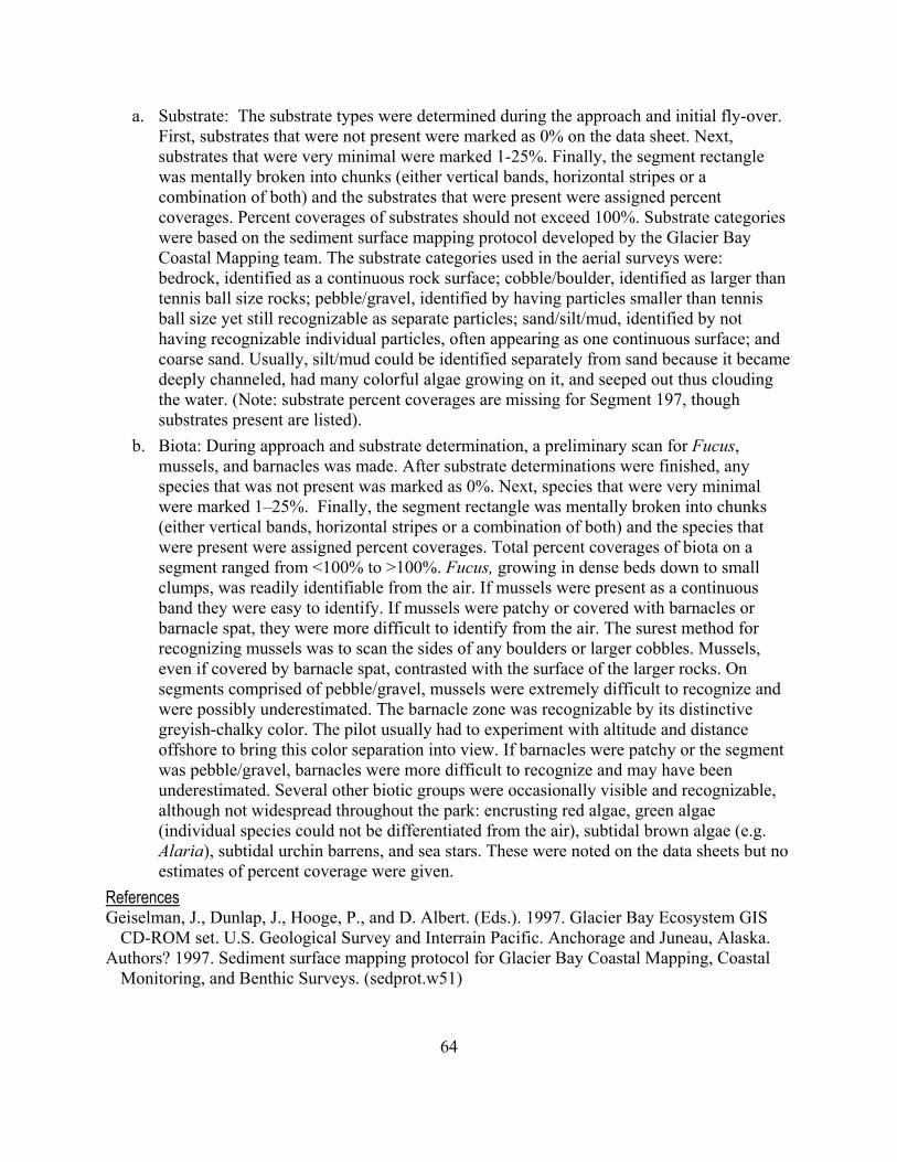
a. Substrate: The substrate types were determined during the approach and initial fly-over. First, substrates that were not present were marked as 0% on the data sheet. Next, substrates that were very minimal were marked 1-25%. Finally, the segment rectangle was mentally broken into chunks (either vertical bands, horizontal stripes or a combination of both) and the substrates that were present were assigned percent coverages. Percent coverages of substrates should not exceed 100%. Substrate categories were based on the sediment surface mapping protocol developed by the Glacier Bay Coastal Mapping team. The substrate categories used in the aerial surveys were: bedrock, identified as a continuous rock surface; cobble/boulder, identified as larger than tennis ball size rocks; pebble/gravel, identified by having particles smaller than tennis ball size yet still recognizable as separate particles; sand/silt/mud, identified by not having recognizable individual particles, often appearing as one continuous surface; and coarse sand. Usually, silt/mud could be identified separately from sand because it became deeply channeled, had many colorful algae growing on it, and seeped out thus clouding the water. (Note: substrate percent coverages are missing for Segment 197, though substrates present are listed).

b. Biota: During approach and substrate determination, a preliminary scan for Fucus, mussels, and barnacles was made. After substrate determinations were finished, any species that was not present was marked as 0%. Next, species that were very minimal were marked 1–25%. Finally, the segment rectangle was mentally broken into chunks (either vertical bands, horizontal stripes or a combination of both) and the species that were present were assigned percent coverages. Total percent coverages of biota on a segment ranged from <100% to >100%. Fucus, growing in dense beds down to small clumps, was readily identifiable from the air. If mussels were present as a continuous band they were easy to identify. If mussels were patchy or covered with barnacles or barnacle spat, they were more difficult to identify from the air. The surest method for recognizing mussels was to scan the sides of any boulders or larger cobbles. Mussels, even if covered by barnacle spat, contrasted with the surface of the larger rocks. On segments comprised of pebble/gravel, mussels were extremely difficult to recognize and were possibly underestimated. The barnacle zone was recognizable by its distinctive greyish-chalky color. The pilot usually had to experiment with altitude and distance offshore to bring this color separation into view. If barnacles were patchy or the segment was pebble/gravel, barnacles were more difficult to recognize and may have been underestimated. Several other biotic groups were occasionally visible and recognizable, although not widespread throughout the park: encrusting red algae, green algae (individual species could not be differentiated from the air), subtidal brown algae (e.g. Alaria), subtidal urchin barrens, and sea stars. These were noted on the data sheets but no estimates of percent coverage were given.

Geiselman, J., Dunlap, J., Hooge, P., and D. Albert. (Eds.). 1997. Glacier Bay Ecosystem GIS CD-ROM set. U.S. Geological Survey and Interrain Pacific. Anchorage and Juneau, Alaska.

References

Authors? 1997. Sediment surface mapping protocol for Glacier Bay Coastal Mapping, Coastal Monitoring, and Benthic Surveys. (sedprot.w51)

65

Figure A-1. Map of the study area showing Glacier Bay proper. Each red dot represents one of the 200m segments sampled during the 1997 aerial survey. The eight “X” marks show sites that were not sampled.

66

Figure A-2. An example of a completed data sheet/segment map from the aerial surveys. The thickened line delineates the 200m segment. The numbers 276 and 278 are the endpoints corresponding to the GPS coordinates given in the upper left corner.

67

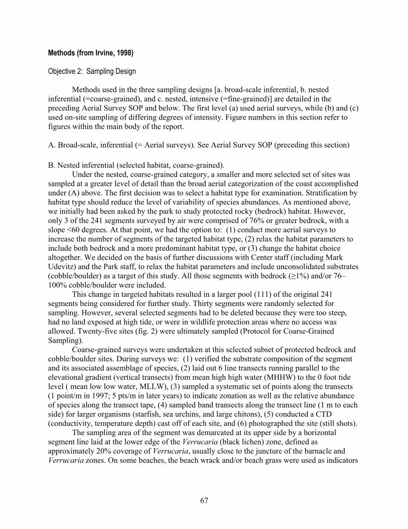
Methods (from Irvine, 1998) Objective 2: Sampling Design

Methods used in the three sampling designs [a. broad-scale inferential, b. nested inferential (=coarse-grained), and c. nested, intensive (=fine-grained)] are detailed in the preceding Aerial Survey SOP and below. The first level (a) used aerial surveys, while (b) and (c) used on-site sampling of differing degrees of intensity. Figure numbers in this section refer to figures within the main body of the report.

A. Broad-scale, inferential (= Aerial surveys). See Aerial Survey SOP (preceding this section) B. Nested inferential (selected habitat, coarse-grained).

Under the nested, coarse-grained category, a smaller and more selected set of sites was sampled at a greater level of detail than the broad aerial categorization of the coast accomplished under (A) above. The first decision was to select a habitat type for examination. Stratification by habitat type should reduce the level of variability of species abundances. As mentioned above, we initially had been asked by the park to study protected rocky (bedrock) habitat. However, only 3 of the 241 segments surveyed by air were comprised of 76% or greater bedrock, with a slope <60 degrees. At that point, we had the option to: (1) conduct more aerial surveys to increase the number of segments of the targeted habitat type, (2) relax the habitat parameters to include both bedrock and a more predominant habitat type, or (3) change the habitat choice altogether. We decided on the basis of further discussions with Center staff (including Mark Udevitz) and the Park staff, to relax the habitat parameters and include unconsolidated substrates (cobble/boulder) as a target of this study. All those segments with bedrock (≥1%) and/or 76–100% cobble/boulder were included.

This change in targeted habitats resulted in a larger pool (111) of the original 241 segments being considered for further study. Thirty segments were randomly selected for sampling. However, several selected segments had to be deleted because they were too steep, had no land exposed at high tide, or were in wildlife protection areas where no access was allowed. Twenty-five sites (fig. 2) were ultimately sampled (Protocol for Coarse-Grained Sampling).

Coarse-grained surveys were undertaken at this selected subset of protected bedrock and cobble/boulder sites. During surveys we: (1) verified the substrate composition of the segment and its associated assemblage of species, (2) laid out 6 line transects running parallel to the elevational gradient (vertical transects) from mean high high water (MHHW) to the 0 foot tide level ( mean low low water, MLLW), (3) sampled a systematic set of points along the transects (1 point/m in 1997; 5 pts/m in later years) to indicate zonation as well as the relative abundance of species along the transect tape, (4) sampled band transects along the transect line (1 m to each side) for larger organisms (starfish, sea urchins, and large chitons), (5) conducted a CTD (conductivity, temperature depth) cast off of each site, and (6) photographed the site (still shots).

The sampling area of the segment was demarcated at its upper side by a horizontal segment line laid at the lower edge of the Verrucaria (black lichen) zone, defined as approximately 20% coverage of Verrucaria, usually close to the juncture of the barnacle and Verrucaria zones. On some beaches, the beach wrack and/or beach grass were used as indicators

68

of the highest tide levels. The horizontal segment line was laid parallel with the shoreline. Six line transects were laid out parallel to the elevational gradient (“vertical“) and perpendicular to the shoreline, running from the horizontal segment line down to mean MLLW. The 0' tide level was determined by using the Tides and Currents computer program (Nautical Software, Inc.) for the sampling date and nearest tide station location (Bartlett Cove, Willoughby Island, Composite Island, or Muir Inlet). The start of the first vertical transect line was determined randomly within the first 33 m of the horizontal segment line; the succeeding transect lines were laid out systematically with respect to the first. One point was sampled at each meter interval of the vertical transects (0, 1, 2 m, etc.): Note: at some sites sampling was increased in density, and in later years, sampling was conducted at 5 points/m. Point sampling was 3-dimensional; all species underlying the point were recorded, from top to bottom, and substrate underlying the point was also recorded.

We expected to sample two sites per low tide, six days of low tides per low tide cycle, for two low tide cycles, giving 24 total expected sites sampled, however, the sites were spaced sufficiently far apart that usually only one site could be sampled on a tide. Data obtained were the percent coverage of sampled species, densities of species counted in the swath surveys, and measures of zonation as reflected in the sampling of the vertical transects.

Initial sampling in May at a site (#63) with very long transects (up to 140m) caused a re-examination of the intensity of sampling that was possible at this level of the survey. Although we had planned originally to sample every 20 cm, we had to scale the sampling to one point per meter in order to be able to complete the sampling of 6 transects by 3 people in one tide. So the one point sampled per meter of transect length became the standard for all coarse-grained level sampling. When we moved up bay and found the transects were considerably shorter, we increased the density of sampling (in order to increase the biological information on a site), but analyses using 1997 data, except where noted, compare all coarse-grained sites at the standard level of sampling (one point/meter).

C. Intensive sampling (selected habitat, fine-grained)

The shift in habitats focused on in Level B (the coarse-grained surveys) had consequences for the selection of sites for Level C (the fine-grained, intensive sampling). The lack of bedrock-dominated segments with slopes less than 60 degrees in the aerial surveys prompted relaxation of the habitat parameters, which resulted in a mixed habitat type becoming the focus in Level B. The 25 Level B sites contained bedrock and/or cobble/boulder substrates, with the mix ranging from 76% or greater bedrock with 1–25% cobble/boulder to 76% or greater cobble/boulder with no bedrock. These sites had been drawn from the pool of all sites containing bedrock, plus all 76% or greater cobble/boulder sites; these latter did not have to have a bedrock component.

The methods of selecting and sampling the sites affect the ability of the park to generalize from the selected sites to other similar sites. We planned to sample six sites at this level. Two factors weighed in narrowing the focus of sites and habitats selected for fine-grained sampling. First, in light of the variability in the habitat mix of the coarse-grained sites, we decided, in consultation with Center and Park staff to concentrate efforts on predominately cobble/boulder sites. In part, the park advocated for consideration of this habitat type (or subset of Level B habitat mix) because of its greater abundance within Glacier Bay proper than low-angle bedrock sites. Only those sites with 76% or greater cobble/boulder were considered for inclusion. Having

69

a bedrock component did not eliminate a site. For example, Site 69 was included, and it contained both 76% or greater cobble/boulder and 1–25% bedrock. Second, we decided to narrow the geographical scope of the sites sampled in this third level, to sites within a region readily accessible from Bartlett Cove by skiff, in order to allow for frequent access. Thus the region from just south of the two arms to approximately the Bartlett Cove level was chosen. Two methods of maintaining inference to the broader pool of sites were apparent. One, to choose a subset of the sites from level B that fit the parameters described above, or two, to draw a new pool of sites from Level A that fit the parameters. We decided to choose a subset of those from level B, in part because we then had the advantage of comparing the two types of sampling at the same sites. In total, below the juncture of the two arms in Glacier Bay proper, were eight sites that had been defined as predominately cobble/boulder by the aerial surveys. One of those in Geike was discarded because the level B surveys had revealed that little cobble/boulder was present. The most southerly geographic outlier was also dropped. This resulted in the selection of six sites that ranged from just south of the two arms to slightly south (but across bay) of Bartlett Cove (fig. 2). The data from these sites is applicable to the range of cobble/boulder habitat within the band or region that the sites occupy, as these sites were originally randomly selected from a pool of the selected habitat type (Level B).

Within-site sampling

All of these sites had been sampled under the coarse-grained regime. The sampling at the fine-grained level included sampling that was similar to the coarse-grained level, although more intensive, plus additional methods of sampling. Locating the site and delineating the horizontal segment tape were accomplished in the same manner as under the coarse-grained procedures.

The within-site sampling included: 1. vertical transects, 2. horizontal transects, 3. band sampling of both vertical and horizontal transects, 4. quadrat sampling, both point-contact and counts of small mobile invertebrates 5. mussel sampling, and 6. fixed quadrats (at one site), 7. photographs of the various sampling units, and 8. some additional marking of the site. The layout of the sampling is depicted in figure 3. 1. Vertical transects: Line transects (vertical transects) were laid out as under the coarse-grained protocol, except 10 instead of 6 were laid out. These transects were positioned parallel to the elevational gradient of the segment, running from the horizontal segment line down to MLLW. The start of the first vertical transect along the horizontal segment tape was determined by choosing a random number between 0 and 20, and the remaining transects were placed systematically relative to the first. Transect lines were draped so as to generally conform to the substrate, rather than being stretched taut. The intention was that all exposed surfaces had an equal probability of being sampled.

70

Point sampling of Vertical (and Horizontal) Transects: Systematically selected points along the vertical transects were sampled to provide estimates of the relative percent cover of biota along the transects, as well as the relative percent cover of underlying substrates. This sampling of points also provides information on the zonation of species. At fine-grained sites, five points were sampled per meter (each 20 cm). Points were sampled 3-dimensionally, noting the species and substrate under each point. The right edge of the tape and the distance hash marks along the tape were used as cross hairs to mark the point. We used knitting needles to facilitate the 3D sampling of the naturally heterogeneous topography for all types of point sampling on the fine-grained level (vertical and horizontal transects, and point-contact quadrats). The knitting needle was used to follow the point perpendicularly from the tape to the substrate. All species underlying the point were recorded, in order from the top down, including multiple “hits“ or layers of the same species. The substrate, which also could be multi-layered, was recorded. Organisms were identified to the lowest taxonomic level possible in field sampling. Some taxa are grouped because they could not be discriminated in the field readily. Substrates were classified according to a modified Wentworth-scale (appendix D1.2, this report). 2. Horizontal transects: (a). Determining the elevations at which horizontal transects and quadrats are set

. As set out in the initial protocol, the total tidal range of a site was going to be determined by assessing the angle of the slope, and multiplying the sine of that angle by the length of the transect (the hypotenuse). We planned to define three elevational zones by dividing the tidal range into thirds. A random number was then going to be used as a multiplier to determine the point within each vertical zone to be sampled, so that each zone was sampled at the same proportionate elevation. The same random number (0.71) was applied to all six sites sampled this round in order to facilitate comparisons between sites. This number set the sampling locations fairly high within each zone.

After determining the tidal heights for sampling along each transect, the actual locations would have been determined through use of the tide programs. Although we initially set up our calculations at Site 63 in this manner, we could not follow the procedure because the high tides were not going to be high enough for us to locate, via the tide tables, the actual locations of the upper horizontal transects. Thus, we modified the procedure in the field, and decided that we had to assume an equal slope and use the distance of the transect line as a proxy of the elevational gradient. So, in the field, the transect length was divided into thirds: a low, middle, and high portion, and a random number (0.71) was multiplied by the length of each third to determine the location for placement of the horizontal transects. For example, if the transect length was 45 m, each 1/3 segment equals 15 m, and the sampling location within each third is the random number (0.71) times 15 m = 10.65 m from the lower end of that third of the transect. This same method was used for all sampling of fine-grained sites in 1997.

71

(b). Laying and sampling horizontal transects

. Horizontal transects were 10 m in length, with the origin at the vertical tape, and the horizontal tape laid to the right as one faces shore. They were run parallel with the water’s edge, unless they were constrained in other ways. For example at site 69, where the bedrock cliff jutted out and made sampling a line parallel with the water impossible, then the transect line was run parallel with the segment line. Point sampling was conducted in the same manner and at the same intensity as for the vertical transects. The sampling under each point was 3D, and was recorded as for the vertical transects.

3. Band sampling: Band surveys were conducted along both vertical and horizontal transects as was done in the coarse-grained sampling. A band one meter to each side (total width of 2 meters) of the transect tape was surveyed for the presence and abundance of specific species, primarily mobile species or larger, rarer species unlikely to be sampled well by point sampling (band species were identified on the species identification list). The number of each band species observed per meter was recorded in the appropriate place on the data sheet. If no band species were observed, that was noted. During the band surveys, substrate was not disturbed, therefore species that more commonly are found in the crevices between cobbles/boulders or under them were probably under-represented (e.g., the six-armed starfish, Leptasterias hexactis).

At some sites, a dense Fucus zone made it difficult to observe band species. In these cases, the bands were scanned from 0 MLLW to the bottom of the Fucus zone (this was noted on the data sheet as well as the distances along the transect line that were searched). In most cases, the Fucus zone was scanned, but Fucus was not moved if it was dense. In 1997, dense Fucus occurred at only a few sites, primarily in the lower bay area. 4. Quadrat sampling (33.3 cm × 33.3 cm quads): Quadrats used were 1/9 m2, with an inner diameter of 33.3 cm per side. A grid of lines was set across the quadrat frames (see fig. 4), and the 36 intersections of the grid created the sampling points. Quadrats were laid out in a systematic manner at the interstices of the vertical and horizontal transects, with the lower edge of the quadrat set along the upper side of the horizontal transect, and the left edge to the right of and along the vertical transect. The quadrat frame was allowed to lie naturally relative to the slope and heterogeneity of the substrate. Occasionally, a quadrat was unstable and had to be supported in order to be assessed. Once the quadrat frame was set, points were sampled perpendicular to the plane of the quadrat. Points were assessed on substrates with slopes up to 90 degrees; substrates where the angle was >90 degrees (underhangs) were ignored. Sampling of points was done in a 3-dimensional manner as for the vertical and horizontal transects. The 3-dimensional assessment of points included counting multiple layers of biota (of the same or different species), and multiple substrates if they were discernible.

Prior to sampling, photos were taken of both the regular quadrat and the adjacent mussel counting quadrat (see below), as the sampling could disturb the position of biota within the quadrat. Usually, a single photo of both the quadrat and adjacent mussel count quadrat was taken. However, if the quadrats lay at different angles separate photos were taken because one photo couldn’t be taken normal (perpendicular) to both.

72

After assessing the point contacts, counts were made of mobile species inside the quadrat, including: chitons, limpets, Nucella spp. (predatory gastropods), nemerteans, sea urchins, and starfish. Counts of mobile species were done to the lowest species distinctions. Limpets <8 mm were lumped into Lottiidae, due to difficulties of accurately identifying small limpets (Nora Foster, pers. comm.). In addition to counts of mobile species, the quadrat was scanned for the presence of other sessile species not counted under the points (including species like Mytilus, whose abundance was highly variable within quadrats). These species were listed as present. Mytilus was not uniformly scanned for presence in 1997.

A small subquadrat (10 × 10 cm) set within the upper left of the 33.3 cm × 33.3 cm quadrat was used to assess the density of littorine snails. In 1997, Littorina scutulata was noted by one observer to be present only at Site 59; L. sitkana having been the predominant species observed. Other observers either saw only L. sitkana, or did not discriminate species.

Barnacle spat. The density of barnacle spat was assessed in the upper left quadrant (5 x 5 cm) of the subquadrat (10 × 10 cm) in which littorines were counted. For 1997, barnacle spat for the quadrat sampling within the fine-grained sampling, which took place late July to August, was defined as barnacles from 0–2 mm diameter. In the coarse-grained sampling, which took place in June to mid-July, barnacle spat was considered 0–1 mm.

5. Mussel quadrat sampling: There were two types of mussel quadrat sampling: (a) sampling within the mussel zone along each vertical transect (with collection of mussels and Fucus), and (b) non-disruptive sampling set systematically along the vertical transects. In both types of mussel sampling, a square 500 cm2 quadrat was used.

(a). Sampling within the mussel zone

followed the layout and sampling procedure of the Exxon Valdez oil spill Nearshore Vertebrate Predator (NVP) Project mussel sampling, with one minor placement deviation noted below. Briefly, the length and location of the mussel zone was defined along each vertical transect, and a random number from 0–1.0 was used as a multiplier to establish the location of the lower horizontal edge of the quadrat within the mussel zone. The random number was multiplied by the length of the mussel zone, then the number was added to the upper edge of the mussel zone to determine the quadrat location relative to the distance down the vertical transect. In our sampling, the 500 cm2 quadrat was displaced one quadrat width to the left of the vertical transect line, so as to not interfere with the second type of mussel quadrat sampling, in which the quadrat was placed adjacent to the vertical transect line (at three locations along each line). One quadrat was sampled per vertical transect line under the first type of mussel sampling. In these quadrats, all mussels and Fucus were collected from the quadrat, placed into a labeled plastic bag, and frozen upon return to the ship, or kept cooled until returned from the field. While removing the mussels and Fucus, if shape of the substrate allowed, then all surfaces were scraped of biota in order to be able to use these clearings to follow recruitment and succession. Back in the lab, mussels were measured, and the length and reproductive status of Fucus plants were recorded.

73

(b). Systematic sampling along the vertical transect lines

involved non-destructive sampling of 500 cm2 quadrats laid out systematically at three points along each vertical transect line. The quadrats were laid out at the intersections of the vertical and horizontal transects, on the left hand side of the vertical transect line, as one faces shoreward. The lower right hand corner of the 500 cm2 quadrat is opposed, across the transect line, from the lower left hand corner of the 33.3 cm × 33.3 cm quadrat, and both have their lower edge at the elevational level defined by the horizontal transect (fig. 3). As mentioned above in the discussion of the 33.3 cm × 33.3 cm quadrat sampling, photos were taken of both quadrats before they were assessed. Three quadrats were placed along each vertical transect line, for a total number of quadrats sampled across the site of 30. Within these quadrats, mussels were counted, but not collected and substrates were not disturbed. Because mussels were sometimes very dense, the quadrat frame was subdivided into three sections with line to facilitate counting, and tally counters were used. Any mussel even partially within the quadrat frame was counted, irrespective of the amount of its shell in the quadrat. All mussels that could be observed without disturbing substrates within the quadrat were counted, including ones in crevices or beneath underhangs, and the smallest identifiable mussels.

6. Fixed quadrats: In 1997, time constraints and design challenges led to fixed quadrats being set up and sampled only at Site 69. Ten fixed quadrats (33.3 cm × 33.3 cm) were laid out and marked on boulders of sufficient size. At this site, the boulders were selected arbitrarily and were spread over the length f the site. These quadrats were sampled in the same manner as the other main quadrat sampling on the beach: 36 points assessed, counts of small mobile invertebrates, subsample counts of littorines and barnacle spat, and scans for other sessile species. Photographs of quadrats are also taken.