Appendix A

Instructions for the ComplexityExperiments

The following list of instructions was given to subjects before the experiment.

After ensuring that subjects understood these instructions, a brief practice session

(on a test sequence) outside the scanner was given before proceeding to the actual

experiment in the scanner.

1. In this experiment, you will see a small "stimulus window" which displays

a grid of 3x3 squares.

2. You have to perform two types of blocks in this experiment: FOLLOW

RANDOM and LEARN SEQUENCE.

3. During the "FOLLOW RANDOM" blocks, one square is illuminated. Please

press as fast as possible the corresponding key on the keypad. The sequence

of lights is randomly generated and so do not try to memorize them.

4. During the "LEARN SEQUENCE" blocks, some of the squares in the 3x3

grid are illuminated. Please clear each target by pressing the corresponding

keys on the keypad. You have to figure out the correct order of key presses

in each set by trial and error.

If you make a mistake in key presses, the program will start, you over

from the beginning of the entire sequence. The sequence remains unal-

tered throughout the experiment. As you practice, please try to memorize

the sequence.

157

5. Before you start a new block you will be shown instructions on the screen

such as "FOLLOW RANDOM" and "LEARN SEQUENCE". Please in-

attention to these instructions so as to perform the appropriate actions.

FOLLOW RANDOM: Clear the targets by pressing the corresponding keys

on the keypad. The sequence of lights is randomly generated and so do not try

to memorize them.

LEARN SEQUENCE: You have to figure out the correct order of key-presses

in each set by trial and error. The sequence remains una.lt.ered throughout, the

experiment. As you practice, please try to memorize the sequence!!

Do not forget to press the keys as fast as you can throughout the

experiment!

Appendix B

Details of Experimental Procedure andFile Formats

This appendix lists the procedure for conducting empirical experimentation and

recording the resulting beliavioaral parameters from experiments. Sample liles

and their formats are described here.

B.I Procedure for conducting the experiment

Parameters used in an experiment are stored in subject files (*.sub) and the

results of an experiment are stored in result files (*.res). Subject files need to be

created for practice and main sessions.

B.I.I Creation of parameter files

Create subject files in the same directory as the executable file Exp. Enter the

following Subject information:

Subject data — f i r s t name

las t name

Results f i l e f i l e name O.res)

The following notations are used in the Subject file:

• "Block" indicates the Block number. Each experiment consists of 52 blocks

•;•'• ;..;,•'.".• arranged in four sessions. Each session contains IS alternating control and

B, 1. Procedure for conductingjhejxperiment

test condition blocks. Every block begins with an instruction screen lastsfor 6 seconds.

• "Label" indicates the type of block - "TrainN" (2x0 or 2x12 or 1x0, test

or sequence learning conditions) or "FolloN" (Control or Baseline Condi-

tion, where subjects pressed one key at a tune by following randomly

generated visual targets, 1x12 random sequence). Each sequence learning

condition will have different .res tiles and they arc identified by the subject's

short name along with the sequence condition (for example, WY2xO.res or

WY2xl2.res or WY4x6.res).

• "Hset#" is a number identifying the hypersct used in the block (21 for

Sequence learning conditions and 20 to 1 for Follow or Control conditions)

by the program.

• "setL" denotes the length of each set in the hypersct - 2 for 2x0 and 4 for

4x6. "HsetL" denotes the length of the liyperset (sequence?) - 12 for 2x12

and 6 for 2x6.

• "HsetT" indicates the liyperset Type. For the Follow blocks it will be

RAN (a random sequence) and Fix (a fixed sequence.1) for test, or sequence

learning blocks.

• "Hand" indicates the type of hand subject used. The entry R denote right,

hand. However, all the subjects in our experiments are right, handed.

• "Key" & "Hset" (Hyperset) The Codes are 2 k 0 for all in this complexity

experiments - No rotations or any other transformations are used.

• All the blocks are in "Mode" 1 (Fight the Sequence and Trial-and-Error key-

press). Mode 2 and 3 are not supported in this complexity experiments.

This mode 1 also used to reset the liyperset during the trial-and-error pro-

cess.

• Block duration length (BDL) is either 18 seconds (Follow or Control blocks)

or 36 seconds (Test or Sequence blocks).

• Set duration is 1.6 sec for 2x6 or 2x12 Sequence Learning blocks in com-

plexity experiments. For 4x6 it, will be 3.2 seconds. On an average, we fixed

maximum of 0.8 seconds for each key-press.

B.2. Subject file __ 160

• "Trials" indicates the number of trials performed during the block.

• "Block_T" denotes the total time taken for perfect trials (where the subject

completed the hyperset successfully). This value does not include the time

taken for incomplete trials (where subject, has committed an error).

• "Err" indicates the number of incomplete trials.

• "Corr" indicates the number of complete trials.

• "Datc_&-Time" records the date and starting time of the block.

B.I.2 Running the Program

We used a modified version of Bapi et al. (2000) experimental program written

in C using Metro works Code warrior compiler for Macintosh Computer (release

1.0).

B.I.3 Practice Session

In each study, the Main session in the scanner is preceded by a practice session of

approximately 1 hr for the complexity experiment to ensure proper understanding

of block instructions and various conditions used in the experimental session.

More practice may be given, if required. The value of "Corr" can be checked by

opening the corresponding practice file (and compare with corresponding total

Trials).

B.2 Subject file

B.2.1 Subject file before the experiment

An example, subject file for 2x6 experiment, is given below:

B.2. Subject file161

B.2.2 Subject file after the experiment

Sample file that is saved after a 2x6 sequence learning task is shown below:

B.3. Result file after the experiment162

B.3 Result file after the experiment

The Result file will contain details of all the trails performed in every block. A

sample file (truncated) for 2x6 task is shown below:

B.3. Result file after the experiment163

B.3. Result file after the experiment

B.4. Post processing of Behavioural Results

B.4 Post processing of Behavioural Results

We developed a C program (using Turbo C Version 3.0) which automatically

computed parameters of interest given a .res file or group of .res files. We gener-

ated two kinds of files .sui and .OM. The .um file is computed for each experiment

and it contains parameters such as total trial time, number of sets completed,

non-zero trials, average key-press time, trials, success rate, successful hypersets

and the number of movements, that are computed block-wise. The .sui hie is a

compressed form of result file, which we used for chunking analysis, the results

of which are reported in the Chapter 6. Some of the parameters of .am file were

used in the behavioural analysis reported in the Chapter 5.

Appendix C

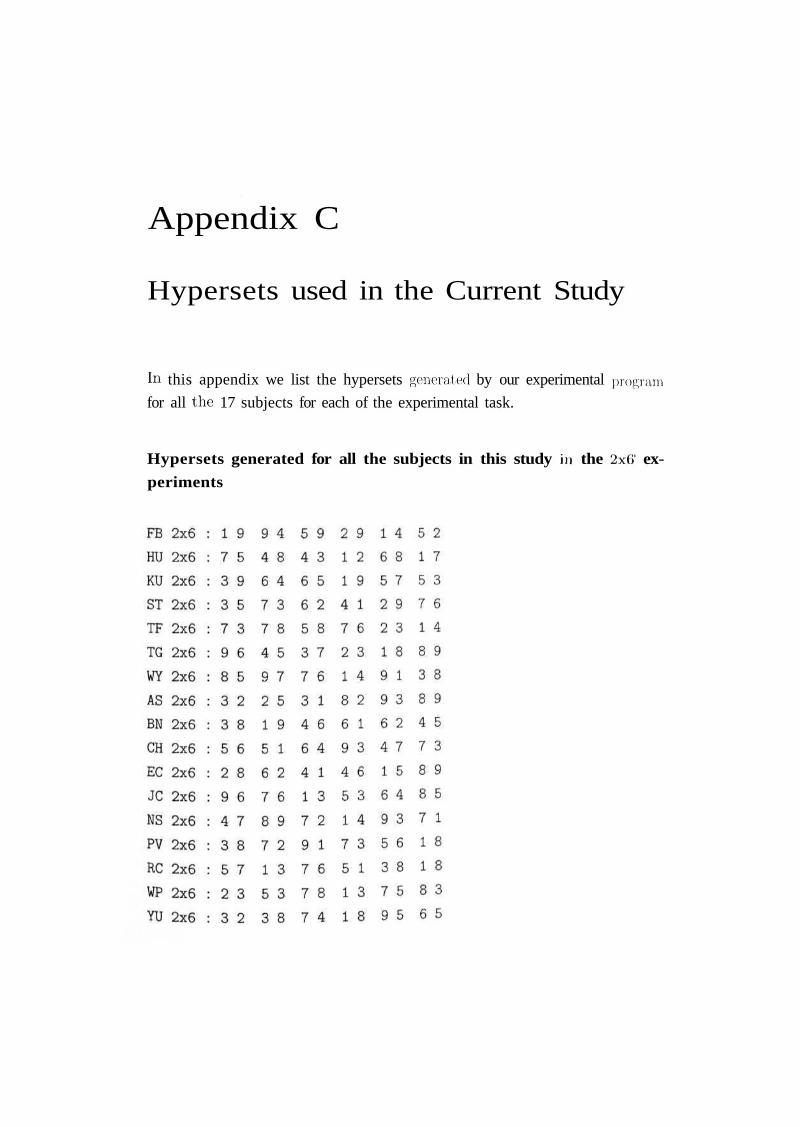
Hypersets used in the Current Study

In this appendix we list the hypersets generated by our experimental program

for all the 17 subjects for each of the experimental task.

Hypersets generated for all the subjects in this study in the 2x(> ex-

periments

167

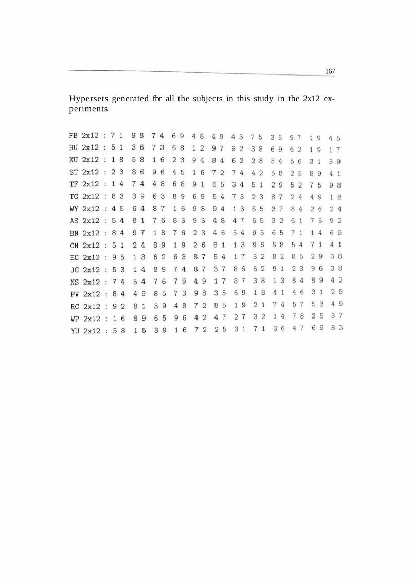
Hypersets generated fbr all the subjects in this study in the 2x12 ex-periments

168

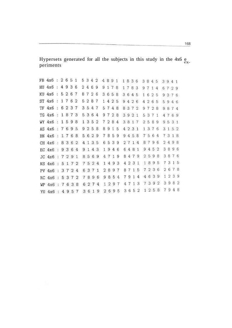
Hypersets generated for all the subjects in this study in the 4x6 eperiments

ex-

Appendix D

Data Analysis Procedure using SPM99

In this appendix, a stcp-by-step procedure is given for performing fMKI data

analysis using the SPM package. A public domain software package, called SPM is

extensively used to analyse functional neuroimaging data,. SPM has an extensive

website at: http://www.fil ion. ucl. ac. uk/spm.

Statistical Parametric Mapping (SPM) refers to the construction and assess-

ment of spatially extended statistical process used to test hypotheses about (neu-

roimaging data from SPECT, PET & fMRI). Also, SPM is a form of data, reduc-

tion, condensing information (in a statistically meaningful way) from a number

of individual scans into a single image volume that can be more; easily viewed

and interpreted.

In the following, sequence of analysis steps to be followed for image analysis is

given. This description also includes a complete listing of menu options in SPM99

along with appropriate values used for our experimental analysis. We adopt a di-

rect instructional guidance approach to present various steps here. Some oi the in-

structions are taken verbatim from the SPM99 manual, Raima ChristofTs online

documentation (available at: http://wim-pHychManS(mUdu^'kulma/SPM99/)

and from various web resources (references listed at the end oi" this Appendix).

D.1. Preprocessing

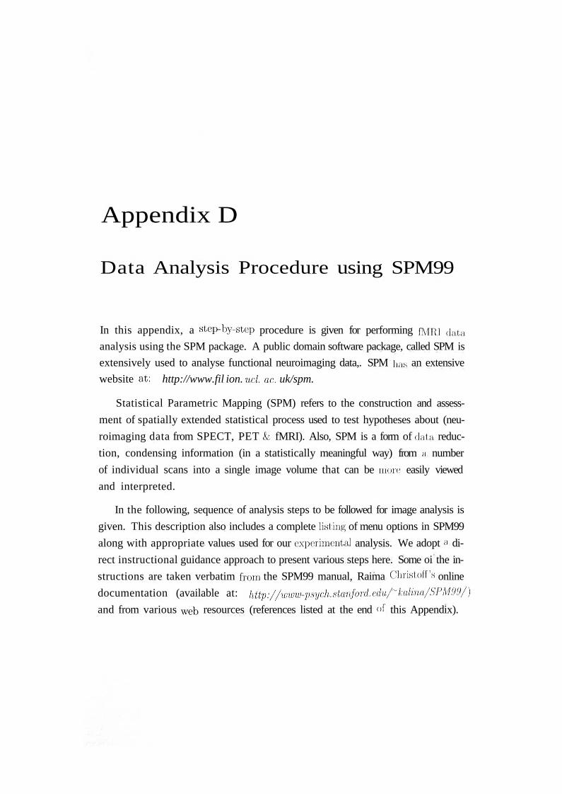
Figure D.I: SPM GUI

SPM99 requires core MATLAB (version 5.2 or higher, Maths Works, Inc.) to

run. The image format used is the simple header and image file formal, of ANA-

LYZE 7.5 (Biomedical Imaging Resource, Mayo Foundation). The graphical user

interface (GUI) of SPM99 is shown in the Figure: D.I. SPM99 separately exam-

ines every voxel (3-dimensional pixel) location across all images, and computes a.

parametric map containing a parameterized value at each voxel. Data, analysis as

implemented in SPM is parametric. Statistics with a known null distribution are

used, such that under the null hypothesis, the probability of obtaining a statistic:

greater than, or equal to, that observed can be computed. The statistical model

used is a special case of the general linear model (Strange. 2000). Several prepro-

cessing steps are required before statistical analysis. The aim of preprocessing is

to reduce artifacts and noise and to perform spatial transformations.

D.I Preprocessing

Spatial transformations are important in many aspects of functional imago anal-

ysis. The first several steps put each image volume into a standardized spatial

reference frame. The final preprocessing step applies a Gaussian spatial filter.

D.1. Preprocessing 171

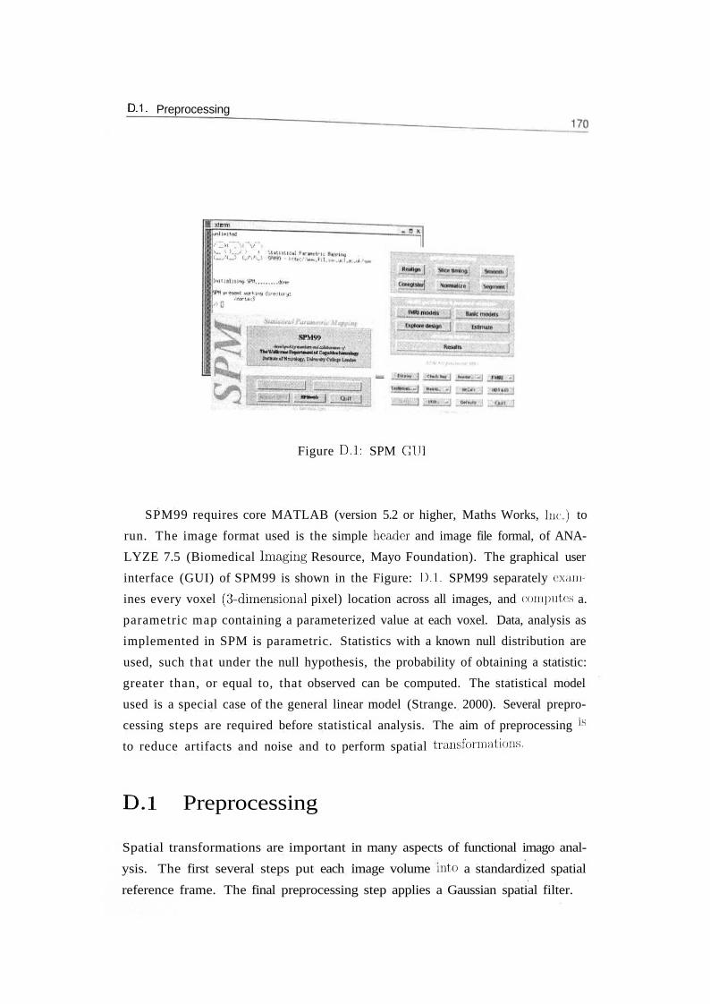
D.I.I Setting the origin and reorientation of images

The goal of setting the origin is to set the origin of functional images to the line

joining anterior commissure to the posterior commissure (AC-PC line) as shown

in the Figure: D.2. The purpose of this is that during the Normalization phase

performed in a later stage, the images from each subject will he warped into a

standardized brain space that has the origin set for the AC. If the origin for a

subject's image is not close to the AC, then the normalization process may be

impeded.

Figure D.2: EP1 Template Image and Locating the Origin

D.1. Preprocessing172

Figure D.3: Images before and after Reorientation

Select "Display" option in the SPM and then select an image to display it. In

the upper part of the screen, there should be 3 boxes showing the 'A orthogonal

views (coronal, axial and sagittal) of the image:

• The upper left box should look like a coronal view

• The lower left box should look like a axial (horizontal) view, with the front

of the brain in the top of the box

• The top right box should display a sagittal view of the? brain, with the front

of the brain on the left side of the box.

Now, adjust the rotations by

• Changing the yaw, if the head is rotated in the axial plane

• • Changing the pitch to set the x axis run through the AC-PC line hi the

v sagittal plane.

D.1. Preprocessing

• Changing the roll if the head is rotated in the coronal plane.

• Now adjust the right(x), Forward(y), and Up(z) values to set the origin

For this purpose, we can use the spm99/templates/epi.img a,s a reference.

Once, everything looks okay, then click on "reorient images" at the bottom of the

display box and select all the functional images to bo reoriented. The results of

reorientation arc shown in the Figure: D.3.

D.1.2 Realignment

The next step is to realign the functional images. Although the subjects are

asked to keep their heads still, movement does occur. This step will align all

the functional images to a single functional image to remove any translations or

rotations within the data set. This is the process used for motion correction.

Select REALIGN

Number of subjects: Enter the appropriate number. Most typically, you would

enter 1 here.

Number of sessions for subject 1: Enter the number of sessions for the entire

experiment.

Scans for subject 1, sessl: select *_l.img- DONE

Scans for subject 1, sess2: select *_2.hng - DONE

... until all sessions (and subjects) are done.

Which option? Select coregister only.Selecting comgister only will cause all files to be realigned by creating *.mat

files that will contain realignment transformations that need to be applied to the

corresponding image files. No new images will b(3 produced (i.e., the image hies

will not be resliccd).

Selecting reshce only will cause new r*.img files to be produced. The *.img

imported will be transformed according to their corresponding *.mat files (given

that they exist) and the resulting images will be written out as r*.i.ng files. No

*.mat files will be created.

Selecting cornier & nslice will both realign the .selected files, ami will ,.n>

duce new files.

• • Realignment works in two stages. First, the first files (*001.nug) from eaeh

D.1. Preprocessing174

session are realigned to the first file of the first session. Second, within each

session, the second, third, etc. (2, • • •, n) images are realigned to the Inst image.

As a consequence, after realignment, all files are realigned to the iirst iile Iron,

t h e first session.

Blue

Green

Red

Translation

XYZ

Rotationpitchrollyaw

Realignment produces text files with estimated motion parameters for each

session. These are rcalignment_params_*.txt. They contain (i columns and each

row corresponds to a *.img file. The columns are the estimated translations in

mm (right, forward, up) and the estimated rotations in radians (pitch, roll, yaw)

that are needed to shift each image file. In sonic1 experiments, the realignment

parameters are used as regressors in the statistical analysis. Realignment param-

eters computed for a single subject are shown in the Figure: D.4. lYanslation

and rotation parameters upto the voxel dimension (in our experiments voxel di-

mension is 3mm) is considered safe for the purpose of statistical analysis.

D.1. Preprocessing175

Figure D.4: Realigninent Parameters

D. 1.3 Coregist r at ion

For studies of a single subject, the sites of activation can be accurately localised

by superimposing them on a high-resolution anatomical structural image oi th«

subject. This requires the registration of the functional images with the aiia^m-

ical image.

D.1. Preprocessing

The goal of eoregistration is to enable the functional images to he overlaid

onto the anatomical (or structural) image of the subject,. This step finds the

transformation that maps the anatomical image into the space of the functional

images. A further use of this registration is that a more precise spatial normaliza-

tion can be achieved by computing it with a more detailed anatomical (structural)

image. A new '.mat' file is created for the anatomical image.

Select COREGISTER

Number of subjects : 1

Which option? coregister only.

Modality of first target image? Select EP1.

The target image is the one to which we coregister. EP1 is the generic option for

functional MR1 images.

Modality of first object image? Select Tl MRL

The object image is the one which is being eoregistered. Select Tl MM if the

structural image looks dark where gray matter should be and bright where white

matter should be. If the structural images has the opposite contrast (bright where

gray matter should be and dark where white matter should be, it, is probably T2

MRI, so select appropriately).

Select target image for subject 1: Select the first functional (EPJ) image -

DONE

Select object image for subject 1: Select the inplane anatomical ;JI) image :

-DONESelect other images for subject 1: - DONE (do not select any images)

If any images are selected as "other", the transformation parameters estimated

to coregister the object to the target image will also be applied to the ''other1'

images.

This step will find the transformation that maps the in plane anatomical

3D image into the space of the functional images (as defined by the; first. EP1

image). A new mat file will be created for the anatomical 3D image. Results of

eoregistration arc shown in Figure: D.5.

To check the coregistration between the functional image and the anatomical

image: Select CHECK REG on the man! menu and select the two .maps.

D.1. Preprocessing 177

CoregistrationX1 = 0.333"X +0.003'Y -0.010*Z -2.176

Y1 = -0.004*X +0.333*Y -0.018'Z -7.341

21 = 0.01CTX +0.018*Y +0.333*Z -27.446

D.1. Preprocessing178

D.1.4 Normalization

Sometimes, it is desirable to warp images from a number of individuals into

roughly the same standard space to allow signal averaging across subjects. A

further advantage of using spatially normalized images is that activation sites

can be reported according to their coordinates within a standard space. The

most commonly adopted coordinate system is the one described by Talairach

and Tournoux (1988).

The normalization process is used to convert the subject's brain into a com-

mon three-dimensional brain space (talairaeh). Normalization facilitates between-

subject analysis to be performed, and allows overlays to be used for examining

data across subjects.

In this process, SPM creates a 2x2x2 voxel size images by default, Also, the

output images will be interpreted as "left is left" and "rigid is ri.ghl" convention,

as popularly used by neurologists. We need to specify if the images need to be

flipped using the "defaults-edit" option and specifying the convention of input

images (i.e. whether Radiological or Neurological).

Select NORMALIZE

Which Option?...: Determine Parameters Only

Number of subjects : 1

Image to determine parameters from : select anatomical 3D.img, DONE

Template to normalize to: Select the Tl image from spmUU/teinplates as the

template image. This is the brain image that is in the standardized space.

The calculated parameters will be stored in the *jsn3d.mat for the anatomical

image.Now, if the parameters seem correct, normalize all the functional images using

this *_sn3d.mat in the following way.

Select NORMALIZE

Which Option?...: Write Normalized Only

Number of subjects : 1

Normalization parameter set : Select the *-sn3d.mat, DONE

Images to write normalized : select all functional images, DONE

Interpolation Method : Sine lnterpolation(9.7:9j;9)

,- This step will create images with a prefix of V for all functional images.

D.1. Preprocessing179

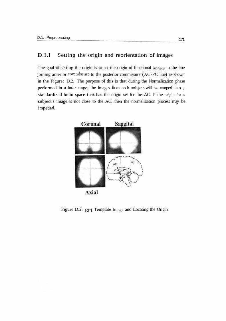
Results of normalization are shown in the Figure: D.G.

Spatial Normalisation

Figure D.6: Normalization

D.I.5 Smoothing

The idea of smoothing is to rcpla.ee the intensity value within each vox,! with

a weighted average (as d e t a i n e d by a gauasian kerne! centered on that pa-

t t a * , voxei) that .corporate* the intensity values of the neighbonng ^

Smoothing U, performed to compensate for residual l,etween-sul,c<:t v a n i

D.2. Statistical Analysis_ _ _ _ _ 180

after normalization.

The matching of the brains m the Normalization step is only possible on a

coarse scale, since there is not necessarily a one-to-one mapping of the cortical

structures between different brains. Because of this, images are smoothed pno,

to the statistical analysis in a, multi-subject study, so that corresponding sit.es of

activation from the different, brains can be superimposed.

Smoothing generally increases the signal relative to noise (SNR). Since, hemo-

dynamic responses are modelled to have a gaussian shape, we need to use a gaus-

sian kernel of size at least twice the voxel size (FWHM of about (i or S min)

for smoothing the functional images. Smoothing also permits tin- application of

Gaussian random field theory at the statistical inference stage.

Select S M O O T H

Smoothing FWHM in mm : 6

Select images to work on : select all normalized images i.e. n*.img, DONE

This step creates images with a prefix of's' for the normalized functional images.

After preprocessing the images, the data are ready for statistical analysis. This

involves two steps: Firstly, statistics indicating evidence against a null hypothesis

of no effect at each voxel are computed. This results in an "image11 of statistics.

Secondly, this statistic image must be assessed, reliably locating voxels where

an effect is exhibited. The hypothesis is framed a,s a design matrix model. The

design matrix is formed by designating a set of columns, which correspond to ex-

perimental conditions of interest (the hypothesis under test) and a set, ol columns

which model effects of no interest.

D.2 Statistical Analysis

Statistical analysis corresponds to the computation of statistical parametric map-

ping using the General linear model (GLM) and theory of ganssian fields. The

GLM is used to specify the conditions in the form of a design matrix, which

defines the experimental design and the nature of hypothesis testing to be imple-

mented. The design matrix has one row for each scan and one column for each

effect (condition) or explanatory variable (e.g. regressor or stimulus function).

The General Linear model is an equation, which expresses the observed re-

sponse variable in terms of a linear combination of explanatory variable* plus a.

well-behaved error term. The general linear model is variously known ns 'analysis

of covariance' or 'multiple regression analysis' and subsumes simpler variants like

the t test for a difference in means. The matrix that contains the explanatory

variables (e.g. designed effects or confounds) is called the design matrix. Each

column in the design matrix corresponds to some effect one ha.s built into the

experiment or that may confound the results.

D.2. Statistical Analysis 181

D.2. Statistical Analysis

The first Follow block occurs after 0 scans from the onset, or ,1 , , U-pimiug of asession

SO A for Sequence : 7

Time to first trial : 2

Parametric modulation : none

Are these Trials : epochs

Events are for a shorter duration and do not, occur in same sequence. Epochs

occur in same sequence and for some amount of time the subjects are doing the

same task, repeatedly.

Type of response : Boxcar

Convolve with hrf? yes

MRI gives us the blood flow signal, but we are interested in the neural activity.

It is possible that the neural response is quicker and the changes in blood How

take place a little later. To account for these? and to find the neural activity from

the MRJ signal, we use the hemodynamic response function (hrf)

Add temporal derivatives : No

Epoch length (scans) for Follow : 2

Epoch length (scans) for Sequence : 5

Interactions among trials : No

user specified regressors : none

This option is used to model specific effects of behaviour with the help of cTplaiia-

tory variable obtained from the behavioural data,. These explanatory variables

could be response time or accuracy or number of movements. In this complex-

ity experiment we used response times (set completion times in 2x(i-4x(i design

matrix and the hyperset completion times in 2x0-2x12 design matric) as 'user-

specified regressors'. The regressor values for each session and then subsequently

for all the images are to be specified using this menu. The regressor values should

correspond to the number of scans in the design matrix. Also, before entering the

regressor values, the regressor values should be convolved (shifted with respect to

scanner repetition time, TR) with hemodynamic response function (hrf) as the

SPM will only do the implicit convolution to the conditions. In this complexity

experiment as TR of the scanner is 0 seconds, we shifted the regressor values only

by one scan.This step creates SPMiMRIDesMtx.mat in the current working directory

SPM_fMRIDesMtx.mat - a file containing the design parameters (onsets, number

182

D.2. Statistical Analysis_ i

of conditions, name of conditions, etc.). It can be used later on for different sub-

jects which have the same design parameters, so that you don't have to specify

them again. To use the file, select fMRl MODELS, and then select estimate a

specified model'.

Estimate a Specified Model

Select the fMRI design matrix SPMJMRIDesMtx.mat

Select scans for session 1 sn_l*.img (44 scans)

Select scans for session 2 - sn.2*.img (44 scans)

Select scans for session 4 sn_4*.img (44 scans)

Remove global effects : None

If you select 'scale' the value in each voxels for a given subfile will be divided

by the global brain mean value for this sn*-file. Global scaling can beneficial,

since it reduced intersubjcct variability and improves the sensitivity al the group

level of analysis. However, it relies on the assumption that the global brain mean

does not correlate with the task. If this assumption is violated, applying global

scaling can cause large areas of the brain to appear as activated. Global scaling

should be applied only with extreme caution. In our experiments, applying the

Global scaling showed huge deactivations (i.e., activation in Contro]>Sequence

tasks). In order to avoid these spurious deactivations, we did not perform Global

Scaling in our analysis.

Temporal auto correlation options:

High Pass Filter : specify

Select 'specify' if you want to filter out the low-frequency components of the sig-

nal. High-pass filtering is usually beneficial, since the low-frequency components

in the fMRI signal contain much more noise than the high-frequency components.

Session cut off period (sees) : 84

T h i s v a l u e i s c o m p u t e d a s , 2 x p e r i o d o f m o s t f r e q u e n t e p o c h - 2 x 7 s c a n s x (>

s e c o n d s = 8 4 s e c o n d s )

Low-pass filter? select 'hrf.

If 'Gaussian' or 'hrf low-pass filter is selected, this will filter out the high-

frequency components in the signal by smoothing the time-series with either

Gaussian or hrf approximation. Low-pass filtering is also known as temporal

smoothing. Theoretically, it is desirable, since the fMRI time-series is autocorre-

D.2. Statistical Analysis" ™ " ' "" ' : ~ •—• ™ ^ .. _ _ „ I C^T

lated, and performing temporal smoothing allows the analysis to take this into

account. However, in practice, temporal smoothing can make the statistical in-

ference overly conservative, thus obscuring otherwise robust activations.

Model intrinsic correlations? none

AR(1) stands for first-order auto-regression model. Modelling intrinsic correla-

tions has the same theoretical goal as temporal smoothing - to take into account

the fact that the fMRI time-series is autocorrelated, which violates the assump-

tion in regression analysis that the different observations arc independent, llnibr-

tunately, it also has the same practical consequence - it can make1 the inferences

overly conservative.

Setup trial specific F contrasts : No

If 'yes' is selected, spin will automatically create F-contnists for each condition

within each session.

Estimate ? Now

Design matrix is shown in Figure: D.7. After estimation is done, the following

important files will be saved in the "analysis" directory (among others):

Y.mad - a file containing the raw data, directly entered from the subfiles. It is

compressed, so it cannot be directly read. The Y.mad file will have the values

for only those voxels that survived the upper F threshold during the analysis.

This threshold is specified through the fMRLUFp variable in the spnidefaults.m

files. If fMRLUFp=l in defaults, all voxels will be present in the Y.mad file If

fMRLUFp=0, Y.mad file will not be written. We set fMRLUFp-J in our exper-

imental analyses. We used in this file in the brain-behaviour correlation (BBC!)

analysis.

xCon.mat - file which contains the information about the contrasts, their names,

values, and so forth. If these parameters are the same for two subjects, the

xCon.mat file can be copied to the second subject directory, so that the param-

eters will only have to entered once.

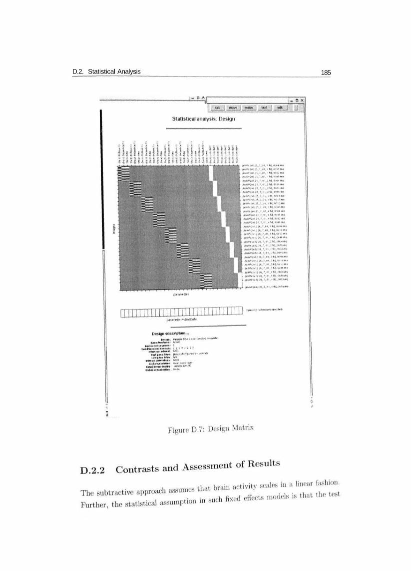
D.2. Statistical Analysis 185

D.2. Statistical Analysis186

blocks are replicated and hence can be averaged and compared to the control

blocks. Higher order effects can be specified by adding non-linear terms to the

GLM. However, this requires that the nature of hypothesized relationship be-

tween the brain activation and an experimental variable is already known.

After the estimation is done, in order to see the results:

Select RESULTS

Select SPM.mat file: Select the SPM.mat file in the "results" directory - done.

SPM contrast manager:Select contrasts ... T-CONTRASTSThe contrasts menu is depicted in Figure1: D.8.

Define New Contrast type in name of contrast, then the contrast values. SUB-

MIT Check the design matrix on the right, if the entered contrast vector is correct,

Select the contrast you want to display DONE, (if more than OIK- contrast

is selected, the conjunction between them will be computed and displayed)

Mask with other contrast(s)?no

D.2. Statistical Analysis•" — — _ 107

If 'yes' is selected, user will be prompted to select another contract from t he same

SPM.mat file. There are two types of masking: inclusive and exclusive. Lot's say

user selected contrast A first, and thru chose to mask it. with contrast B. Inclu-

sive masking should display everything in contrast. A plus tin- voxels activated by

contrast B and not activated by contrast A. Exclusive masking will display those

voxels activated by contrast A that are also activated by contrast, H. More tech-

nically, exclusive masking is used to reject the voxels where the null hypothesis

(A-B) can be rejected.

Corrected height threshold? no

If 'yes' is selected, only voxels surviving the corrected threshold value will bedisplayed.

The individual voxels in most ncuroimaging modalities (PET, fMR], EEC, MEG

etc.) are heavily correlated with neighboring voxels. This means a correction

for multiple comparisons is needed. The traditional way of doing this is to use

some version of a Bonferroni correction. However, due to large number of voxels

involved, a straightforward implementation would severely reduce the estimated

number of degrees of freedom. The major contribution of the SPM99 authors was

to figure out a statistically valid approach. To the extent, that the image data,

approximate a Random Gaussian Field, the theories behind Random Gaussian

Fields can be used to yield valid statistical comparisons of images. This assump-

tion is assured by applying a Gaussian smoothing filter to the image data in the

pre-processing stages.

Threshold p value Enter the uncorrected p value you would like to use as

threshold. Typically 0.001 for individual analysis.

Extent threshold voxels Enter the min number of voxels that a cluster should

have in order to be displayed. For the least conservative estimate, enter 0.

Go through the above steps for each contrast. This will create con*.img files in

the analysis directory, which are needed for the group analysis level.

Press Volume to show the summary of local maxima. The Figure: I).9 depicts

fMRI results along with the details of activated voxels. The brain activations in

three sections (sagittal, coronal and axial) will be obtained by pressing Overlays

menu item. This option requires to choose an 'image to be rendered on'. Figure:

D.10 is an example in which the brain activity is overlaid on one of our subject's

normalized high resolution image.

D.2. Statistical Analysis188

D.3. Random Effects Analysis (RFX)189

Figure D.10: Visualising activations overlaid on subject's high resolution image

D.3 Random Effects Analysis (RFX)

The purpose of the Random Effects analysis is to find the areas that are activated

in much the same way in all subjects, as opposed to the fixed effects model which

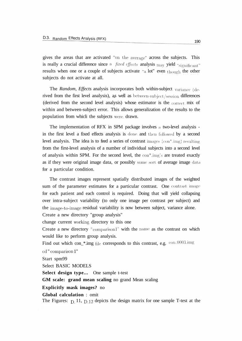
D.3. Random Effects^Analysis (RFX)190

gives the areas that are activated «011 t,he average" across the subjects. This

is really a crucial difference since a .fixed effects analysis may yield significant1

results when one or a couple of subjects activate "a lot" even though the other

subjects do not activate at all.

The Random, Effects analysis incorporates both within-subject variance (de-

rived from the first level analysis), a,s well as between-subject/session differences

(derived from the second level analysis) whose estimator is the correct mix of

within and between-subject error. This allows generalization of the results to the

population from whicli the subjects were1 drawn.

The implementation of RFX in SPM package involves a two-level analysis -

in the first level a fixed effects analysis is done- and then followed by a second

level analysis. The idea is to feed a series of contrast images (eon*.img) resulting

from the first-level analysis of a number of individual subjects into a second level

of analysis within SPM. For the second level, the con*.hng\s are treated exactly

as if they were original image data, or possibly some sort, of average image data

for a particular condition.

The contrast images represent spatially distributed images of the weighted

sum of the parameter estimates for a particular contrast. One contrast image

for each patient and each control is required. Doing that will yield collapsing

over intra-subject variability (to only one image per contrast per subject) and

the image-to-image residual variability is now between subject, variance alone.

Create a new directory "group analysis"

change current working directory to this one

Create a new directory "comparisonT with the name as the contrast on which

would like to perform group analysis.

Find out which con_*.img hie corresponds to this contrast, e.g. conJHKl.limg

ed " comparison 1"

Start spm99

Select BASIC MODELS

Select design type... One sample t-test

GM scale: grand mean scaling no grand Mean scaling

Explicitly mask images? no

Global calculation : omitThe Figures: D. 11, D.I2 depicts the design matrix for one sample T-test at the

D.3. Random Effects Analysis (RFX) 191

second level (RFX analysis) and fMRI results for an example cas

Figure D.ll: Design Matrix in RFX for one Sample T-Test

D.4. Sources and Further Reading192

Figure D.I2: Results from Random Effects (RFX) analysis for one Sample T~Tcst

D.4 Sources and Further Reading

The material in this appendix has been compiled from the following resources:

• SPM99: Protocols, Tools, and Documentation by Kalina Christoff, Depart-

ment of Psychology, Stanford University

http://www-psych.stanford.edu/" kalina/SPM99/

SPM99 Preprocessing Protocolhttp://www-psych.stanford.edu/~kalina/

SPM99/Protocols/spm99_prepros_])rot.htnil

SPM99 Analysis Protocol

D.4. Sources andfurther Reading

http://www-psycli.stanford.edii/~kalina/

SPM99/Protocols/spm99_analysis_prot,htnil

• SPM Resources by Terry Oakcs, W.M. Keek Laboratory for functional

Brain Imaging and Behaviour, University of Wisconsin. Madison

http://www.keck.waisniaii.wisc.edu/~()akos/spin/spin_n»s«)urt-t's.htinlSPM99 Introduction

http://www.keck.waisnian.wisc.e(lu/^oaJws/spin/SPM99..1ntr(»(lu(li()n.p(lfSPM How-tos

http://www.keck. waismaii.wis(\(xlu/~()ak<\s/spii)/si)iii..h()w_t()s.hl.inlRandom Effects Analysis

http://www.keck.waisman.wise.(Hlu/"'oakes/s])in/spiiLrandom efiects.html

• Preprocessing Steps for SPM99 by Todd Handy, Center for Cognitive Neu-

roscience, Dartmouth College

http://www.(]artmoutli.edu/^cogneuro/i)pn()tes.btnil

• SPM Statistics and other Tutorials by Matthew Brett,, MRO Cognition and

Brain Sciences Unit, University of Cambridge.

http://www.mrc-cbu.cain.a(Mik/Inia,ging/CorniT)on/l.til.oriM.]H.sljf.nil

For Further Reading, the following annotated bibliography by the authors of SPM

can be consulted.Statistical Parametric Mapping: An Annotated Bibliography

W.D. Penny, J. Ashburner, S. Kiebel, R. Henson, D.E. Glaser, C. Phillips and

Karl J. Priston.Wellcome Department of Imaging Neuroseience, University College London.

http://www.fil.iori.ucl.ac.uk/spm/bib.htiii

Appendix E

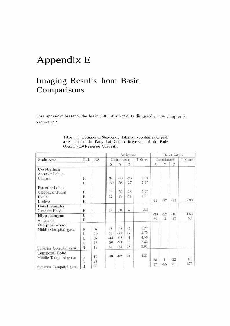
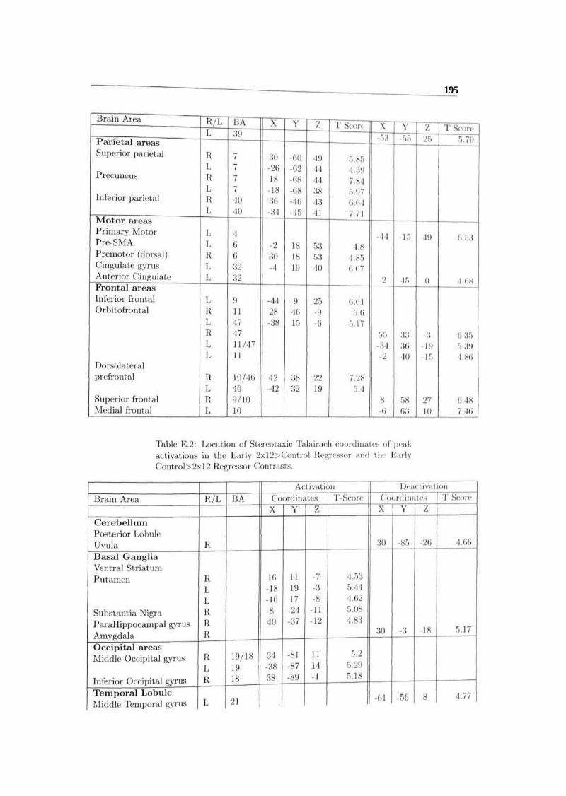
Imaging Results from BasicComparisons

This appendix presents the basic comparison results discussed in the Clin.pt.rr 7,

Section 7.2.

Table E.I: Location of Stereotaxic Talairach coordinates of peakactivations in the Early 2xO>Control Regressor and the EarlyControl>2xG Regressor Contrasts.

195

196

197

198

Table E.4: Location of Stereotaxie Talairach coordinates of peakactivations in the Consolidation 2x(i>Control Regressur and theConsolidation Control>2x6 Regressor Contrasts.

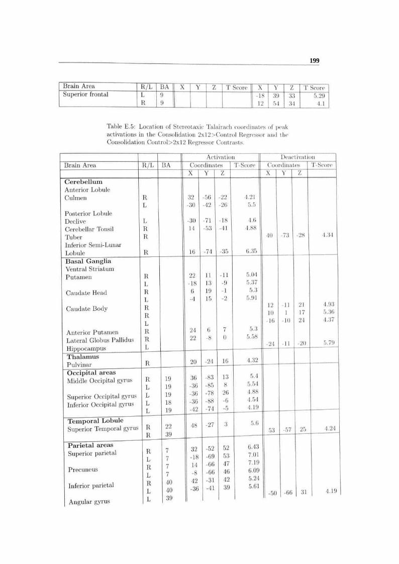
199

200

201

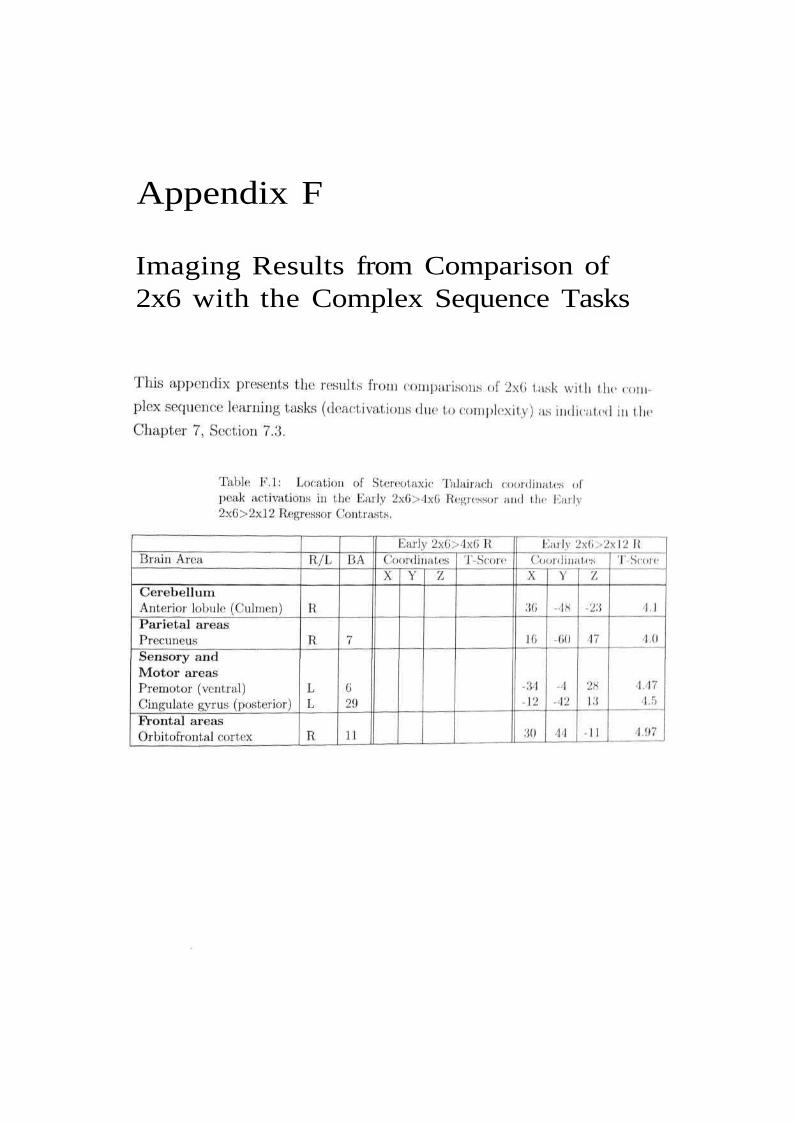
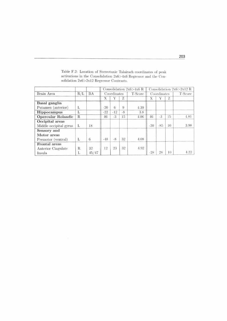
Appendix F

Imaging Results from Comparison of2x6 with the Complex Sequence Tasks

203

CURRICULUM VITAE

PAMMI V. S. CHANDRASEKHAREmail: pvscs@yahoo.com, vscpammi@gmail.com

EDUCATION:

Ph.D. Computer Science, (Thesis Submitted)Department of Computer and Information Sciences,University of Hyderabad, India

M.Phil. Computational Physics, (August 1998 - December 1999)School of Physics, University of Hyderabad, India

M.Sc. Electronics, (August 1995 - April 1997)School of Physics, University of Hyderabad, India

B.Sc. Mathematics, Physics and Electronics, (July 1992-April 1995)Andhra University, Waltair, India

ACADEMIC AND INDUSTRIAL EXPERIENCE:

April 2002 - September 2003:Research Assistant,Indo-Japanese project titled "Sequence learning: An fMRI Investigation"funded by Kawato Dynamic Brain Project (KDB), Exploratory Researchfor Advance Technology (ERATO), Japan Science and TechnologyAgency, Japan at University of Hyderabad, India.

July 2001-August 2001:Visiting Researcher,ATR International, Kyoto, Japan invited by KDB Project, ERATO, .1ST.

November 1998 - March 2001:Research Fellow (Junior and Senior),Research Centre Imarat (RCI), Defence Research and DevelopmentOrganization (DRDO), Hyderabad, India

May 1997-June 1998:Junior Engineer (Research and Development),Research and Development Division (R&D), APEL RadioCommunication Systems (Pvt.) Ltd., Secunderabad, India.