appendix c: lab guide for stata - central web server...
TRANSCRIPT

QUANT 2 Stata Lab Guide – 2011 - Page 50
Appendix C: Lab Guide for Stata 2011
1. The Lab Guide is divided into sections corresponding to class lectures. Each section includes both a review, which everyone should complete and an exercise, which is intended to get you started working more creatively with the commands.
2. We have provided a number of data sets, which you are welcome to use for the exercises. These include: quant2_science3.dta, quant2_hsb3.dta, quant2_nes3.dta, quant2_addhealth3.dta, and quant2_gss3.dta. Codebooks are at the end of the Lab Guide. You can also use your own data for the exercises.
3. As you work through the exercises, feel free to skip questions and explore commands in ways we have not suggested.
4. We provide a few examples of interpretation in the review sections. These are in shaded
boxes.
5. Although the command window can be used for exploring new commands, exercises should always be completed using do‐files. If you are not sure how to use a do‐file, see Getting Started Using Stata for help.
6. This lab guide uses a few auxiliary packages separate from the Stata’s base program. If you are running the do‐files on a computer outside the lab, make sure you have the following two packages set up:
1) spost9_ado from http://www.indiana.edu/~jslsoc/stata 2) estout from http://repec.org/bocode/e
To install an auxiliary package, type findit packagename in the command window and hit Enter (for example, “findit spost9_ado”). Then double click on the link of the desired package to install. For more information, refer to page 8 in Getting Started Using Stata.

QUANT 2 Stata Lab Guide – 2011 - Page 51
Contents
Section 1: Linear Regression – REVIEW ............................................................................................................52
Section 1: Linear Regression – EXERCISE..........................................................................................................56
Section 2: Models for Binary Outcomes – REVIEW ..........................................................................................57
Section 2: Models for Binary Outcomes – EXERCISE ........................................................................................65
Section 3: Testing and Assessing Fit – REVIEW.................................................................................................66
Section 3: Testing and Assessing Fit – EXERCISE ..............................................................................................71
Section 4: Models for Ordinal Outcomes – REVIEW.........................................................................................72
Section 4: Models for Ordinal Outcomes – EXERCISE ......................................................................................78
Section 5: Models for Nominal Outcomes – REVIEW.......................................................................................79
Section 5: Models for Nominal Outcomes – EXERCISE.....................................................................................88
Section 6: Models for Count Outcomes – REVIEW...........................................................................................89
Section 6: Models for Count Outcomes – EXERCISE.........................................................................................99

QUANT 2 Stata Lab Guide – 2011 - Page 52
Section 1: Linear Regression – REVIEW The commands from this section are in quant201a-linear-rev.do. ___1.1R) Set‐up your do‐file. capture log close log using quant201a-linear-rev, replace text // program: quant201a-linear-rev.do // task: Review 1 - Linear Regression // project: QUANT 2 // author: your name \ today's date // #1 // program setup version 11 clear all set linesize 80 matrix drop _all ___1.2R) Load the Data. use quant2_scireview3, clear ___1.3R) Examine the Data and Select Variables. First, describe the dataset to see a list of variables and some information about the dataset. This command: describe Produces this output: . describe Contains data from quant2_scireview3.dta obs: 264 Biochemist data for review - Some data artificially constructed vars: 34 11 May 2009 10:14 size: 16,632 (99.9% of memory free) (_dta has notes) -------------------------------------------------------------------------------- storage display value variable name type format label variable label -------------------------------------------------------------------------------- id float %9.0g ID number cit1 int %9.0g Citations in PhD yrs -1 to 1 ::output deleted:: jobprst float %9.0g prstlb Rankings of University Job. * indicated variables have notes --------------------------------------------------------------------------------Sorted by: jobprst Use keep to select the dependent variable totpub and the three independent variables, faculty, enrol, and phd, which we use in the regression models later. keep totpub faculty enrol phd ___1.4R) Drop cases with missing data and verify. Use misschk to review the missing data. Then, use the variable you generated with the gen(m) option to keep only those observations that are not missing on any of your selected variables.

QUANT 2 Stata Lab Guide – 2011 - Page 53
misschk, gen(m) tab mnumber keep if mnumber==0 Finally, you’ll describe the data to verify that you’ve kept only the variables you want and deleted the missing cases. These command: describe tab1 faculty enrol phd, m Produce this output: . misschk, gen(m) Variables examined for missing values # Variable # Missing % Missing -------------------------------------------- 1 enrol 0 0.0 2 phd 0 0.0 3 faculty 0 0.0 4 totpub 0 0.0 Missing for | which | variables? | Freq. Percent Cum. ------------+----------------------------------- ____ | 264 100.00 100.00 ------------+----------------------------------- Total | 264 100.00 Missing for | how many | variables? | Freq. Percent Cum. ------------+----------------------------------- 0 | 264 100.00 100.00 ------------+----------------------------------- Total | 264 100.00 . keep if mnumber==0 (0 observations deleted) . describe Contains data from quant2_scireview3.dta obs: 264 Biochemist data for review - Some data artificially constructed vars: 4 18 May 2009 10:14 size: 3,960 (99.9% of memory free) (_dta has notes) -------------------------------------------------------------------------------- storage display value variable name type format label variable label -------------------------------------------------------------------------------- enrol byte %9.0g Years from BA to PhD. phd float %9.0g Prestige of Ph.D. department.

QUANT 2 Stata Lab Guide – 2011 - Page 54
faculty byte %9.0g faclbl 1=Faculty in University totpub byte %9.0g Total Pubs in 9 Yrs post-Ph.D. -------------------------------------------------------------------------------- Sorted by: Note: dataset has changed since last saved . tab1 faculty enrol phd, miss -> tabulation of faculty 1=Faculty | in | University | Freq. Percent Cum. ------------+----------------------------------- 0_NotFac | 123 46.59 46.59 1_Faculty | 141 53.41 100.00 ------------+----------------------------------- Total | 264 100.00 :: output deleted :: ___1.5R) Regression. Specifying a model is simple, with the dependent variable listed first, followed by independent variables. This command: regress totpub faculty enrol phd Produces this output: . regress totpub faculty enrol phd Source | SS df MS Number of obs = 264 -------------+------------------------------ F( 3, 260) = 10.77 Model | 3519.43579 3 1173.14526 Prob > F = 0.0000 Residual | 28326.1968 260 108.946911 R-squared = 0.1105 -------------+------------------------------ Adj R-squared = 0.1003 Total | 31845.6326 263 121.086055 Root MSE = 10.438 ------------------------------------------------------------------------------ totpub | Coef. Std. Err. t P>|t| [95% Conf. Interval] -------------+---------------------------------------------------------------- faculty | 5.227261 1.297375 4.03 0.000 2.672561 7.78196 enrol | -1.174879 .4465778 -2.63 0.009 -2.054249 -.2955094 phd | 1.506904 .6442493 2.34 0.020 .2382931 2.775514 _cons | 9.982767 3.33341 2.99 0.003 3.418849 16.54668 ------------------------------------------------------------------------------ ___1.6R) Obtain Standardized Coefficients. listcoef lists the estimated coefficients for a variety of regression models. The help option includes details on the meaning of each coefficient. This command: listcoef, help Produces this output: . listcoef, help regress (N=264): Unstandardized and Standardized Estimates Observed SD: 11.003911 SD of Error: 10.437764

QUANT 2 Stata Lab Guide – 2011 - Page 55
------------------------------------------------------------------------------- totpub | b t P>|t| bStdX bStdY bStdXY SDofX -------------+----------------------------------------------------------------- faculty | 5.22726 4.029 0.000 2.6125 0.4750 0.2374 0.4998 enrol | -1.17488 -2.631 0.009 -1.6955 -0.1068 -0.1541 1.4432 phd | 1.50690 2.339 0.020 1.5147 0.1369 0.1377 1.0052 ------------------------------------------------------------------------------- b = raw coefficient t = t-score for test of b=0 P>|t| = p-value for t-test bStdX = x-standardized coefficient bStdY = y-standardized coefficient bStdXY = fully standardized coefficient SDofX = standard deviation of X ___1.7R) Close Log File and Exit Do File. log close exit

QUANT 2 Stata Lab Guide – 2011 - Page 56
Section 1: Linear Regression – EXERCISE The file quant201b-linear-ex.do contains an outline of this exercise. ___1.1) Set‐up your do‐file. ___1.2) Load the data. ___1.3) Examine the data and select variables. Choose one continuous dependent variable and at least
three independent variables (make sure one is binary and one is continuous) to use in a regression analysis.
___1.4) Drop cases with missing data and verify. ___1.5) Run an OLS regression. ___1.6) Obtain x‐standardized, y‐standardized, and fully standardized coefficients. ___1.7) Interpretation (you should write the answers as if they were part of a research paper)
___a. Interpret at least one unstandardized coefficient. ___b. Interpret at least one x‐standardized, one y‐standardized and one fully standardized
coefficient. ___1.8) Close log and exit do‐file

QUANT 2 Stata Lab Guide – 2011 - Page 57
Section 2: Models for Binary Outcomes – REVIEW The file quant202a-binary-rev.do contains these Stata commands. ___2.1R) Set‐up your do‐file. capture log close log using quant202a-binary-rev, replace text // program: quant202a-binary-rev.do // task: Review 2 - Binary Regression // project: QUANT 2 // author: your name \ today's date // #1 // program setup version 11 clear all set linesize 80 matrix drop _all ___2.2R) Load the Data. use quant2_scireview3, clear ___2.3R) Examine data, select variables, drop missing, and verify. describe keep faculty fellow phd mcit3 mnas misschk , gen(m) tab mnumber keep if mnumber==0 :: output deleted :: These commands: summarize tab1 faculty fellow phd mcit mnas Produce the following output: . summarize Variable | Obs Mean Std. Dev. Min Max -------------+-------------------------------------------------------- fellow | 264 .4128788 .4932865 0 1 mcit3 | 264 20.71591 25.44536 0 129 mnas | 264 .0833333 .2769103 0 1 phd | 264 3.181894 1.00518 1 4.66 faculty | 264 .5340909 .4997839 0 1 . tab1 faculty fellow phd mcit mnas -> tabulation of faculty 1=Faculty |

QUANT 2 Stata Lab Guide – 2011 - Page 58
in | University | Freq. Percent Cum. ------------+----------------------------------- 0_NotFac | 123 46.59 46.59 1_Faculty | 141 53.41 100.00 ------------+----------------------------------- Total | 264 100.00 :: output deleted :: ___2.4R) Binary Logit Model. As with regression, the dependent variable is listed first. A probit model is run by simply changing logit to probit. This command: logit faculty fellow phd mcit3 mnas Produces this output: . logit faculty fellow phd mcit3 mnas Iteration 0: log likelihood = -182.37674 Iteration 1: log likelihood = -164.019 Iteration 2: log likelihood = -163.55936 Iteration 3: log likelihood = -163.55534 Iteration 4: log likelihood = -163.55534 Logistic regression Number of obs = 264 LR chi2(4) = 37.64 Prob > chi2 = 0.0000 Log likelihood = -163.55534 Pseudo R2 = 0.1032 ------------------------------------------------------------------------------ faculty | Coef. Std. Err. z P>|z| [95% Conf. Interval] -------------+---------------------------------------------------------------- fellow | 1.250155 .2767966 4.52 0.000 .7076434 1.792666 phd | -.0637186 .1471307 -0.43 0.665 -.3520894 .2246522 mcit3 | .0206156 .0071255 2.89 0.004 .0066498 .0345814 mnas | .3639082 .5571229 0.65 0.514 -.7280327 1.455849 _cons | -.5806031 .4498847 -1.29 0.197 -1.462361 .3011547 ------------------------------------------------------------------------------ ___2.5R) Store the estimation results. It is sometimes handy to store estimation results to call up later in table format. You can do this using the command eststo. Here we store the estimates with the name estlogit. eststo estlogit ___2.6R) Predicted Probabilities. We can compute and plot predicted probabilities for our observed data. Here we pick the name prlogit for the new variable that contains predicted values. Note that a predicted score is calculated for each case in the sample. These commands: predict prlogit label var prlogit "Logit: Predicted Probability" sum prlogit dotplot prlogit graph export quant202a-binary-rev-fig1.emf , replace

QUANT 2 Stata Lab Guide – 2011 - Page 59
Produce this output: . predict prlogit (option p assumed; Pr(faculty)) . label var prlogit "Logit: Predicted Probability" . sum prlogit Variable | Obs Mean Std. Dev. Min Max -------------+-------------------------------------------------------- prlogit | 264 .5340909 .1828654 .3035647 .9665072 . dotplot prlogit
.2.4
.6.8
1Lo
git:
Pre
dict
ed P
roba
bilit
y
0 10 20 30 40Frequency
___2.7R) Predict Specific Probabilities. prvalue computes the predicted value of our dependent variable given a set of values for our independent variables. Use the x(variables = values) option to set the values at which the variables will be examined. Use rest(mean) to set the other independent variables at their means. Note that whereas the command predict creates a new variable that contains the predicted score for each case in the sample, prvalue computes a predicted probability for a case with certain characteristics and hence does not create a new variable. This command: prvalue, x(fellow=1 mnas=1) rest(mean) Produces this output: . prvalue , x(fellow=1 mnas=1) rest(mean) logit: Predictions for faculty Confidence intervals by delta method 95% Conf. Interval Pr(y=1_Facult|x): 0.7786 [ 0.5931, 0.9642] Pr(y=0_NotFac|x): 0.2214 [ 0.0358, 0.4069] fellow phd mcit3 mnas x= 1 3.1818939 20.715909 1

QUANT 2 Stata Lab Guide – 2011 - Page 60
The predicted probability of obtaining a faculty position for a scientist with both a fellowship and a mentor who was a member of the national association of scientists (NAS) and who is otherwise average is 0.78. ___2.8R) Table of predicted probabilities. A table of predicted probabilities for different combinations of values of independent variables can be obtained with the command prtab. This command: prtab fellow mnas Produces this output: . prtab fellow mnas logit: Predicted probabilities of positive outcome for faculty ------------------------------- Postdoctor | Mentor NAS: al fellow: | 1=yes,0=no. 1=y,0=n. | 0_OutNAS 1_InNAS -----------+------------------- 0_NoFellow | 0.4119 0.5019 1_Fellow | 0.7097 0.7786 ------------------------------- fellow phd mcit3 mnas x= .41287879 3.1818939 20.715909 .08333333 ___2.9R) Discrete Change. prvalue can also be used to compute the discrete change at specific values of the independent variables when the save and dif options are used. By default, discrete changes are calculated holding all other variables at their mean. Note that I use the quietly option to suppress the output of the first prvalue command since the information is repeated when the second prvalue command is executed. These commands: quietly prvalue , x(fellow=1) rest(mean) save label(Fellow) prvalue , x(fellow=0) rest(mean) dif label(NotFellow) Produce this output: . quietly prvalue , x(fellow=1) rest(mean) save label(Fellow) . prvalue , x(fellow=0) rest(mean) dif label(NotFellow) logit: Change in Predictions for faculty Confidence intervals by delta method Current Saved Change 95% CI for Change Pr(y=1_Facult|x): 0.4192 0.7159 -0.2967 [-0.4156, -0.1777] Pr(y=0_NotFac|x): 0.5808 0.2841 0.2967 [ 0.1777, 0.4156] fellow phd mcit3 mnas Current= 0 3.1818939 20.715909 .08333333 Saved= 1 3.1818939 20.715909 .08333333 Diff= -1 0 0 0

QUANT 2 Stata Lab Guide – 2011 - Page 61
A scientist who receives a post‐doctoral fellowship has a .30 higher probability of being on faculty at a university than a scientist who does not receive a fellowship, holding other variables at their mean values. This difference is significant (95% CI: 0.18, 0.42). ___2.10R) Discrete Change 2. prchange computes the discrete change for all independent variables but does not calculate a confidence interval for the discrete change. As with prvalue, values for specific independent variables can be set using the x() and rest() options. The help option provides a key. This command: prchange , rest(mean) help Produces this output: . prchange , rest(mean) help logit: Changes in Probabilities for faculty min->max 0->1 -+1/2 -+sd/2 MargEfct fellow 0.2967 0.2967 0.3003 0.1516 0.3097 phd -0.0576 -0.0154 -0.0158 -0.0159 -0.0158 mcit3 0.4775 0.0051 0.0051 0.1292 0.0051 mnas 0.0881 0.0881 0.0899 0.0250 0.0902 0_NotFac 1_Facult Pr(y|x) 0.4526 0.5474 fellow phd mcit3 mnas x= .412879 3.18189 20.7159 .083333 sd(x)= .493287 1.00518 25.4454 .27691 Pr(y|x): probability of observing each y for specified x values Avg|Chg|: average of absolute value of the change across categories Min->Max: change in predicted probability as x changes from its minimum to its maximum 0->1: change in predicted probability as x changes from 0 to 1 -+1/2: change in predicted probability as x changes from 1/2 unit below base value to 1/2 unit above -+sd/2: change in predicted probability as x changes from 1/2 standard dev below base to 1/2 standard dev above MargEfct: the partial derivative of the predicted probability/rate with respect to a given independent variable
A standard deviation increase in the number of mentor’s citations (centered around the mean) increases the predicted probability of obtaining a faculty position by .13 for a scientist who is average on all other characteristics. ___2.11R) Plot predicted probabilities. It is often useful to compute predicted probabilities across the range of a continuous variable for two groups and then plot them. We do this using prgen. prgen generates a series of new variables containing predicted values and confidence intervals. The new variables begin with the stem you indicate in the option gen(). These commands: prgen mcit3, x(fellow=1) rest(mean) from(0) to(130) gen(fel1) gap(5) ci prgen mcit3, x(fellow=0) rest(mean) from(0) to(130) gen(fel0) gap(5) ci label var fel1p1 “Fellow” label var fel0p1 “Not a Fellow”
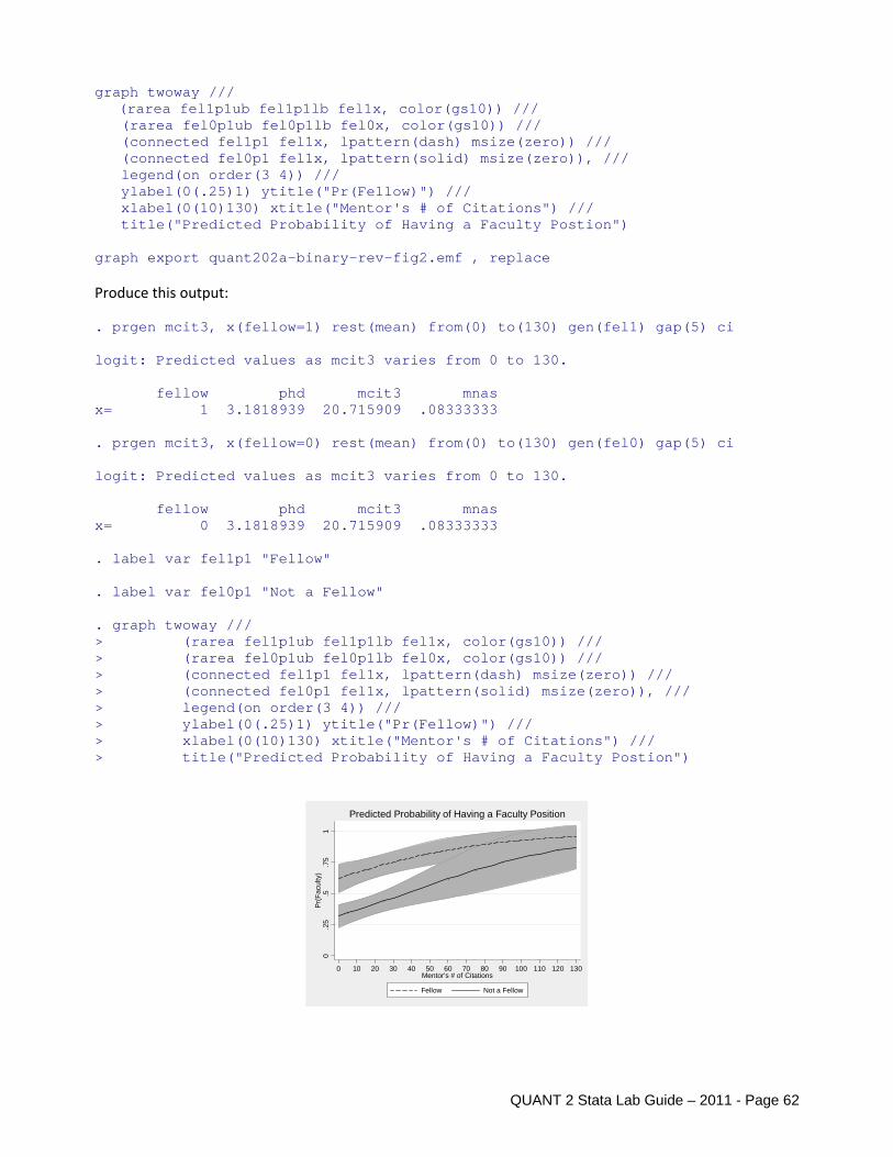
QUANT 2 Stata Lab Guide – 2011 - Page 62
graph twoway /// (rarea fel1p1ub fel1p1lb fel1x, color(gs10)) /// (rarea fel0p1ub fel0p1lb fel0x, color(gs10)) /// (connected fel1p1 fel1x, lpattern(dash) msize(zero)) /// (connected fel0p1 fel1x, lpattern(solid) msize(zero)), /// legend(on order(3 4)) /// ylabel(0(.25)1) ytitle("Pr(Fellow)") /// xlabel(0(10)130) xtitle("Mentor's # of Citations") /// title("Predicted Probability of Having a Faculty Postion") graph export quant202a-binary-rev-fig2.emf , replace Produce this output: . prgen mcit3, x(fellow=1) rest(mean) from(0) to(130) gen(fel1) gap(5) ci logit: Predicted values as mcit3 varies from 0 to 130. fellow phd mcit3 mnas x= 1 3.1818939 20.715909 .08333333 . prgen mcit3, x(fellow=0) rest(mean) from(0) to(130) gen(fel0) gap(5) ci logit: Predicted values as mcit3 varies from 0 to 130. fellow phd mcit3 mnas x= 0 3.1818939 20.715909 .08333333 . label var fel1p1 "Fellow" . label var fel0p1 "Not a Fellow" . graph twoway /// > (rarea fel1p1ub fel1p1lb fel1x, color(gs10)) /// > (rarea fel0p1ub fel0p1lb fel0x, color(gs10)) /// > (connected fel1p1 fel1x, lpattern(dash) msize(zero)) /// > (connected fel0p1 fel1x, lpattern(solid) msize(zero)), /// > legend(on order(3 4)) /// > ylabel(0(.25)1) ytitle("Pr(Fellow)") /// > xlabel(0(10)130) xtitle("Mentor's # of Citations") /// > title("Predicted Probability of Having a Faculty Postion")
0.2
5.5
.75
1P
r(Fac
ulty
)
0 10 20 30 40 50 60 70 80 90 100 110 120 130Mentor's # of Citations
Fellow Not a Fellow
Predicted Probability of Having a Faculty Position

QUANT 2 Stata Lab Guide – 2011 - Page 63
For an average scientist, receiving a fellowship increases the probability of being employed as a faculty member when mentor’s citations are below 50 or so. At higher levels of mentor’s citations, there is no significant difference between scientists who received a fellowship and those who did not. In general, the probability of being employed as a faculty member increases as the number of mentor’s citations increases and receiving a fellowship appears to be particularly useful when mentor’s citations are low. ___2.12R) Computing Odds Ratios. The factor change in the odds as well as the standardized factor change can be obtained with the command listcoef. Note that listcoef can also be run after estimating a probit model, but odds ratios cannot be computed for this model. Instead standardized beta coefficients are listed. This command: listcoef, help Produces this output: . listcoef, help logit (N=264): Factor Change in Odds Odds of: 1_Facult vs 0_NotFac ---------------------------------------------------------------------- faculty | b z P>|z| e^b e^bStdX SDofX -------------+-------------------------------------------------------- fellow | 1.25015 4.517 0.000 3.4909 1.8528 0.4933 phd | -0.06372 -0.433 0.665 0.9383 0.9380 1.0052 mcit3 | 0.02062 2.893 0.004 1.0208 1.6897 25.4454 mnas | 0.36391 0.653 0.514 1.4389 1.1060 0.2769 ---------------------------------------------------------------------- b = raw coefficient z = z-score for test of b=0 P>|z| = p-value for z-test e^b = exp(b) = factor change in odds for unit increase in X e^bStdX = exp(b*SD of X) = change in odds for SD increase in X SDofX = standard deviation of X ___2.13R) Compare the coefficients from Logit and Probit. Run a probit model using the same variables and store the results. Use eststo to store the estimation results and esttab to list these side‐by‐side with the estimation results from the logit model. Note that the logit estimates are around 1.7 times as large as the probit estimates. Why is this? These commands: probit faculty fellow phd mcit3 mnas eststo estprobit esttab estlogit estprobit , mtitles(logit probit) Produce these results: . probit faculty fellow phd mcit3 mnas, nolog Probit regression Number of obs = 264 LR chi2(4) = 37.28 Prob > chi2 = 0.0000 Log likelihood = -163.73838 Pseudo R2 = 0.1022 ------------------------------------------------------------------------------ faculty | Coef. Std. Err. z P>|z| [95% Conf. Interval] -------------+----------------------------------------------------------------

QUANT 2 Stata Lab Guide – 2011 - Page 64
fellow | .763915 .1675687 4.56 0.000 .4354863 1.092344 phd | -.0392676 .0897914 -0.44 0.662 -.2152556 .1367203 mcit3 | .0118642 .003994 2.97 0.003 .0040362 .0196922 mnas | .2299521 .3252353 0.71 0.480 -.4074975 .8674016 _cons | -.3450294 .2743016 -1.26 0.208 -.8826506 .1925919 ------------------------------------------------------------------------------ . eststo estprobit . esttab estlogit estprobit , mtitles(logit probit) -------------------------------------------- (1) (2) logit probit -------------------------------------------- fellow 1.250*** 0.764*** (4.52) (4.56) phd -0.0637 -0.0393 (-0.43) (-0.44) mcit3 0.0206** 0.0119** (2.89) (2.97) mnas 0.364 0.230 (0.65) (0.71) _cons -0.581 -0.345 (-1.29) (-1.26) -------------------------------------------- N 264 264 -------------------------------------------- t statistics in parentheses * p<0.05, ** p<0.01, *** p<0.001 ___2.14R) Close Log File and Exit Do File.
log close exit

QUANT 2 Stata Lab Guide – 2011 - Page 65
Section 2: Models for Binary Outcomes – EXERCISE The file quant202b-binary-ex.do contains an outline of this exercise. ___2.1) Set‐up your do‐file ___2.2) Load your data. ___2.3) Examine the data and select your variables. Choose one binary dependent variable and at least
three independent variables (make sure one is binary and one is continuous). Drop cases with missing data and verify.
___2.4) Estimate a binary logit model ___2.5) Store the results of the logistic regression. ___2.6) Predict probabilities for each observation. Make sure to label the new variable created by
predict. ___2.7) Use prvalue to compute the predicted probability at some specific value of the independent
variables. Interpret this. ___2.8) Create a table of predicted probabilities using prtab. ___2.9) Use prvalue,save and prvalue,dif to calculate a discrete change. Interpret this. ___2.10) Use prchange to calculate the discrete changes. Interpret a few of these. ___2.11) Use prgen to plot the predicted probabilities over the range of a continuous variable for the
two levels of a binary variable (this is similar to what is done on page 59 of the notes). Interpret this.
___2.12) Obtain the factor change coefficients using listcoef, help. Interpret at least one of the
unstandardized and one the standardized factor change coefficients. ___2.13) Compare the logit and probit coefficients by listing them side‐by‐side in a table. Why are the
unstandardized coefficients different? ___2.14) Close log and exit do‐file

QUANT 2 Stata Lab Guide – 2011 - Page 66
Section 3: Testing and Assessing Fit – REVIEW The file quant203a-testing-rev.do contains these Stata commands. ___3.1R) Set‐up your do‐file. capture log close log using quant203a-testing-rev, replace text // program: quant203a-testing-rev.do // task: Review 3 - Testing & Fit // project: QUANT 2 // author: your name \ today's date // #1 // program setup version 11 clear all set linesize 80 matrix drop _all ___3.2R) Load the Data. use quant2_scireview3, clear ___3.3R) Examine data, select variables, drop missing, and verify. keep faculty female fellow phd mcit3 mnas misschk, gen(m) tab mnumber keep if mnumber==0 tab1 faculty female fellow phd mcit3 mnas ___3.4R) z‐scores are produced with the standard estimation commands. This command: logit faculty female fellow phd mcit3 mnas, nolog Produces this output: . logit faculty female fellow phd mcit3 mnas, nolog Logistic regression Number of obs = 264 LR chi2(5) = 41.72 Prob > chi2 = 0.0000 Log likelihood = -161.51514 Pseudo R2 = 0.1144 ------------------------------------------------------------------------------ faculty | Coef. Std. Err. z P>|z| [95% Conf. Interval] -------------+---------------------------------------------------------------- female | -.5869003 .2911944 -2.02 0.044 -1.157631 -.0161698 fellow | 1.118336 .2844612 3.93 0.000 .5608027 1.67587 phd | .002004 .1521298 0.01 0.989 -.2961648 .3001729 mcit3 | .0190813 .0072584 2.63 0.009 .0048551 .0333075 mnas | .3537104 .5652778 0.63 0.531 -.7542137 1.461634 _cons | -.5004836 .4539085 -1.10 0.270 -1.390128 .3891607 ------------------------------------------------------------------------------

QUANT 2 Stata Lab Guide – 2011 - Page 67
___3.5R) Single Coefficient Wald Test. After estimation, the command test can compute a Wald test that a single coefficient is equal to zero. This command: test female Produces this output: . test female ( 1) female = 0 chi2( 1) = 4.06 Prob > chi2 = 0.0439 ___3.6R) Multiple Coefficients Wald Test. We can also test if multiple coefficients are equal to zero. This command: test mcit3 mnas Produces this output: . test mcit3 mnas ( 1) mcit3 = 0 ( 2) mnas = 0 chi2( 2) = 7.78 Prob > chi2 = 0.0204
The hypothesis that the effects of mentor’s citations and mentor’s status as an NAS member are simultaneously equal to zero can be rejected at the .05 level (χ2=7.78, df=2, p=.02). ___3.7R) Equal Coefficients Wald Test. We can test that multiple coefficients are equal. This command: test mcit3 = mnas Produces this output: . test mcit3 = mnas ( 1) mcit3 - mnas = 0 chi2( 1) = 0.35 Prob > chi2 = 0.5545 ___3.8R) LR Test ‐ Store the Estimation Results. To conduct a likelihood ratio test you begin by storing the estimation results using the eststo command. We run the base model and then store the estimates with the name base. logit faculty female fellow phd mcit3 mnas eststo base ___3.9R) Single Coefficient LR Test. To test that the effect of female is zero, run the base model without female and then compare with the full model using lrtst estname1 estname2. These commands: logit faculty fellow phd mcit3 mnas

QUANT 2 Stata Lab Guide – 2011 - Page 68
eststo nofemale lrtest base nofemale Produce this output: . logit faculty fellow phd mcit3 mnas :::output deleted::: . eststo nofemale . lrtest base nofemale Likelihood-ratio test LR chi2(1) = 4.08 (Assumption: nofemale nested in base) Prob > chi2 = 0.0434 ___3.10R) Multiple Coefficients LR Test. To test if the effects of mcit3 and mnas are jointly zero, run the comparison model without these variables, store the estimation results, and then compare models using lrtest. These commands: logit faculty female fellow phd eststo nomcit3mnas lrtest base nomcit3mnas Produces this output: . logit faculty female fellow phd :::output deleted::: . eststo nomcit3mnas . lrtest base nomcit3mnas Likelihood-ratio test LR chi2(2) = 9.19 (Assumption: nomcit3mnas nested in base) Prob > chi2 = 0.0101 ___3.11R) LR Test All Coefficients are Zero. To test that all of the regressors have no effect, we estimate the model with only an intercept, store the estimation results again, and compare the models using lrtest. Note that this test statistic is identical to the one produced at the top of the estimation output for the full model (see page 16). These commands: logit faculty estimates store intercept lrtest base intercept Produce this output: . logit faculty :::output deleted::: . eststo intercept . lrtest base intercept Likelihood-ratio test LR chi2(5) = 41.72 (Assumption: intercept nested in base) Prob > chi2 = 0.0000 ___3.12R) Fit Statistics. fitstat computes measures of fit for your model. The save option saves the computed measures in a matrix for subsequent comparisons. dif compares the fit measures of the current model with those of the saved model. Here we compare the base model to the model without mcit3 and
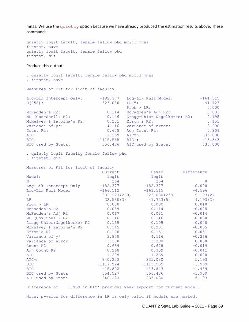
QUANT 2 Stata Lab Guide – 2011 - Page 69
mnas. We use the quietly option because we have already produced the estimation results above. These commands: quietly logit faculty female fellow phd mcit3 mnas fitstat, save quietly logit faculty female fellow phd fitstat, dif Produce this output: . quietly logit faculty female fellow phd mcit3 mnas . fitstat, save Measures of Fit for logit of faculty Log-Lik Intercept Only: -182.377 Log-Lik Full Model: -161.515 D(258): 323.030 LR(5): 41.723 Prob > LR: 0.000 McFadden's R2: 0.114 McFadden's Adj R2: 0.081 ML (Cox-Snell) R2: 0.146 Cragg-Uhler(Nagelkerke) R2: 0.195 McKelvey & Zavoina's R2: 0.201 Efron's R2: 0.151 Variance of y*: 4.116 Variance of error: 3.290 Count R2: 0.678 Adj Count R2: 0.309 AIC: 1.269 AIC*n: 335.030 BIC: -1115.565 BIC': -13.843 BIC used by Stata: 356.486 AIC used by Stata: 335.030 . quietly logit faculty female fellow phd . fitstat, dif Measures of Fit for logit of faculty Current Saved Difference Model: logit logit N: 264 264 0 Log-Lik Intercept Only -182.377 -182.377 0.000 Log-Lik Full Model -166.112 -161.515 -4.596 D 332.223(260) 323.030(258) 9.193(2) LR 32.530(3) 41.723(5) 9.193(2) Prob > LR 0.000 0.000 0.010 McFadden's R2 0.089 0.114 -0.025 McFadden's Adj R2 0.067 0.081 -0.014 ML (Cox-Snell) R2 0.116 0.146 -0.030 Cragg-Uhler(Nagelkerke) R2 0.155 0.195 -0.040 McKelvey & Zavoina's R2 0.145 0.201 -0.055 Efron's R2 0.120 0.151 -0.031 Variance of y* 3.850 4.116 -0.266 Variance of error 3.290 3.290 0.000 Count R2 0.659 0.678 -0.019 Adj Count R2 0.268 0.309 -0.041 AIC 1.289 1.269 0.020 AIC*n 340.223 335.030 5.193 BIC -1117.524 -1115.565 -1.959 BIC' -15.802 -13.843 -1.959 BIC used by Stata 354.527 356.486 -1.959 AIC used by Stata 340.223 335.030 5.193 Difference of 1.959 in BIC' provides weak support for current model. Note: p-value for difference in LR is only valid if models are nested.

QUANT 2 Stata Lab Guide – 2011 - Page 70
___3.13R) Plotting Influential Cases Using Cook’s Distance. To plot outliers, we first compute Cook’s distance using the command predict, dbeta. Then we sort our data in some meaningful way (here we choose to sort by phd). Next we generate a new variable called index whose values correspond to the rank order of phd (because of the way the data are sorted). Finally we plot the Cook’s distance against the rank order of phd. These commands: quietly logit faculty female fellow phd mcit3 mnas predict cook, dbeta sort phd gen index = _n twoway scatter cook index, ysize(1) xsize(2) ///
xlabel(0(100)300) ylabel(0(.2)1., grid) /// xscale(range(0, 300)) yscale(range(0, 1.)) /// xtitle("Observation Number") /// msymbol(none) mlabel(index) mlabposition(0) graph export quant203a-testing-rev-fig1.emf, replace Produce this graph:
1234
567891011121314151617
181920
2122
2324252627282930
3132333435363738394041424344
454647484950515253545556575859606162636465666768697071
72737475767778798081
8283
84858687888990919293949596979899100101102103104105106107108109110111112113114115116117
118119120121122123124
125126127128129130131132
133134135136137138139140
141
142143144145146147148149150151152153154
155156157158159160161162163
164
165166167168169170
171172173174175176177178
179180181182183184185186
187188189190191192193
194
195196197
198
199200201
202
203204
205
206
207
208209210211212
213214215216
217
218219220221222223
224225226
227228
229
230
231
232
233
234
235
236
237238239240241
242
243244245246247
248249
250251
252253254255256
257258259
260261
262
263
264
0.2
.4.6
.81
Pre
gibo
n's
dbet
a
0 100 200 300Observation Number
___3.14) Close the Log File and exit Do File. log close exit

QUANT 2 Stata Lab Guide – 2011 - Page 71
Section 3: Testing and Assessing Fit – EXERCISE The file quant203b-testing-ex.do contains an outline of this Exercise. If you have done a lot of work already with testing, start with question 3.11 on examining outliers and influential observations. ___3.1) Set‐up your do‐file ___3.2) Load your data ___3.3) Examine the data and select your variables. Select one binary dependent variable and at least
three independent variables. Again be sure to include at least one binary and one continuous independent variable. Drop cases with missing data and verify.
___3.4) Run a logit on the full model. ___3.5) Test the hypothesis that the effect of one of your independent variables is zero using the z‐
statistic. What is your conclusion? Use eststo to store estimation results. ___3.6) Use test to conduct a Wald test of the same hypothesis as in 3.5. How is the specific value of
the Wald test related to the z‐test in 3.5? ___3.7) Now use the likelihood ratio test for the same hypothesis in 3.6. ___3.8) Test the hypothesis that the effects of two of your independent variables are simultaneously
equal to zero using the Wald test. What is your conclusion? ___3.9) Now use the likelihood ratio test for the same hypothesis in 3.8. ___3.10) Use fitstat to compare two of your models. Which model do you prefer and why? ___3.11) Using your preferred model, use methods for detecting outliers and influential observations to
evaluate weaknesses in your model. Based on what you find as extreme and/or influential cases, revise your model. Evaluate the revised model in terms of outliers and influential observations. Did things change?
___3.12) Close log & exit.

QUANT 2 Stata Lab Guide – 2011 - Page 72
Section 4: Models for Ordinal Outcomes – REVIEW The file quant204a-ordinal-rev.do contains these Stata commands. ___4.1R) Set‐up your do‐file. capture log close log using quant204a-ordinal-rev, replace text // program: quant204a-ordinal-rev.do // task: Review 4 - Ordinal Regression // project: QUANT 2 // author: your name \ today's date // #1 // program setup version 11 clear all set linesize 80 matrix drop _all ___4.2R) Load the Data. use quant2_scireview3, clear ___4.3R) Examine data, select variables, drop missing, and verify. Make sure to look at the distribution of the outcome variable, in this case jobprst. describe keep jobprst pub1 phd female misschk, gen(m) tab mnumber keep if mnumber==0 summarize tab jobprst , m :::output deleted::: . tab jobprst , m Rankings of | University | Job. | Freq. Percent Cum. ------------+----------------------------------- 1_Adeq | 29 10.98 10.98 2_Good | 128 48.48 59.47 3_Strg | 93 35.23 94.70 4_Dist | 14 5.30 100.00 ------------+----------------------------------- Total | 264 100.00 ___4.4R) Ordered Logit. ologit and oprobit work in the same way. We only show ologit, but you might want to try what follows using oprobit. This command: ologit jobprst pub1 phd female Produces this output: . ologit jobprst pub1 phd female

QUANT 2 Stata Lab Guide – 2011 - Page 73
Iteration 0: log likelihood = -294.86055 Iteration 1: log likelihood = -255.97269 Iteration 2: log likelihood = -254.53567 Iteration 3: log likelihood = -254.51518 Iteration 4: log likelihood = -254.51518 Ordered logistic regression Number of obs = 264 LR chi2(3) = 80.69 Prob > chi2 = 0.0000 Log likelihood = -254.51518 Pseudo R2 = 0.1368 ------------------------------------------------------------------------------ jobprst | Coef. Std. Err. z P>|z| [95% Conf. Interval] -------------+---------------------------------------------------------------- pub1 | .1078786 .0481107 2.24 0.025 .0135833 .2021738 phd | 1.130028 .1444046 7.83 0.000 .8470003 1.413056 female | -.6973579 .2617103 -2.66 0.008 -1.210301 -.1844152 -------------+---------------------------------------------------------------- /cut1 | .9274554 .4268201 .0909033 1.764007 /cut2 | 4.003182 .4996639 3.023859 4.982505 /cut3 | 7.034637 .6296717 5.800503 8.26877 ------------------------------------------------------------------------------ ___4.5R) Predicted Probabilities in Sample. Use predict to compute predicted probabilities after ologit or oprobit. The predict command creates as many new variables as there are categories of the outcome variable so you will need to provide, in this case, 4 variable names that correspond to the four outcome categories. The first variable contains the probability associated with the lowest outcome; the second, the probability associated with the second outcome; and so on. Remember to label the newly created variables. Here are the commands: predict jpad jpgo jpst jpdi label var jpad "OLM Pr(Adeq)" label var jpgo "OLM Pr(Good)" label var jpst "OLM Pr(Strg)" label var jpdi "OLM Pr(Dist)" ___4.6R) Plot Predictions. An easy way to see the range of predictions is with the command dotplot. These commands: dotplot jpad jpgo jpst jpdi, ylabel(0(.25).75) graph export quant204a-ordinal-rev-fig1.emf , replace Produce and save this plot:

QUANT 2 Stata Lab Guide – 2011 - Page 74
0.2
5.5
.75
OLM Pr(Adeq) OLM Pr(Good) OLM Pr(Strg) OLM Pr(Dist)
___4.7R) Predict Specific Probabilities. prvalue computes the predicted value of the dependent variable given a set of values for the independent variables. Use the x() and rest() options to set the values at which the variables will be examined. These commands: prvalue, x(female=1 phd=4) rest(mean) Produce this output: . prvalue, x(female=1 phd=4) rest(mean) ologit: Predictions for jobprst Confidence intervals by delta method 95% Conf. Interval Pr(y=1_Adeq|x): 0.0413 [ 0.0170, 0.0655] Pr(y=2_Good|x): 0.4412 [ 0.3436, 0.5388] Pr(y=3_Strg|x): 0.4683 [ 0.3690, 0.5676] Pr(y=4_Dist|x): 0.0492 [ 0.0182, 0.0802] pub1 phd female x= 2.3219697 4 1
For a female from a distinguished university who is otherwise average, the probability of obtaining a distinguished job is .05. ___4.8R) Graph Predicted Probabilities. Graphing predictions at specific, substantively informative values is usually more effective than the dotplot of sample predictions above. Here we use the command prgen to generate variables for graphing. We consider women from distinguished PhD programs (phd=4) and show how predicted probabilities are influenced by publications. prgen creates variables for both the predicted probabilities and the cumulative probabilities. Here we use scatter to plot the cumulative probabilities. These commands: prgen pub1, x(female=1 phd=4) rest(mean) from(0) to(20) gen(pubpr) label var pubprs1 "Pr(<=Adeq)" label var pubprs2 "Pr(<=Good)" label var pubprs3 "Pr(<=Strg)" label var pubprs4 "Pr(<=Dist)" graph twoway (connected pubprs1 pubprs2 pubprs3 pubprs4 pubprx, /// xtitle("Publications: PhD yr -1 to 1") ///

QUANT 2 Stata Lab Guide – 2011 - Page 75
xlabel(0(5)20) ylabel(0(.25)1, grid) /// msymbol(Oh Dh Sh Th) name(tmp2, replace) /// text(.01 .75 "Adeq", place(e)) /// text(.22 5 "Good", place(e)) /// text(.60 10 "Strong", place(e)) /// text(.90 17 "Dist", place(e))), /// legend(off) graph export quant204a-ordinal-rev-fig2.emf , replace Produce and save this plot:
Adeq
Good
Strong
Dist
0.2
5.5
.75
1C
umul
ativ
e P
r(Job
Pre
stig
e)
0 5 10 15 20Publications: PhD yr -1 to 1
for Females from Distinguished PhD ProgramsJob Prestige and Pubications
___4.9R) Compute the Marginal and Discrete Change. prchange computes the marginal and discrete change at specific values of the independent variables. By default, the discrete and marginal change is calculated holding all other variables at their means. Values for specific independent variables can be set using the x() and rest() options. These commands: prchange, x(female=1 phd=4) rest(mean) Produce this output: . prchange, x(female=1 phd=4) rest(mean) pub1 Avg|Chg| 1_Adeq 2_Good 3_Strg 4_Dist Min->Max .2056791 -.04531779 -.36604039 .21180955 .19954866 -+1/2 .01346503 -.00426875 -.0226613 .02188173 .00504833 -+sd/2 .03470229 -.01103957 -.05836502 .05635044 .01305413 MargEfct .01346829 -.00426717 -.0226694 .02189 .00504658 phd Avg|Chg| 1_Adeq 2_Good 3_Strg 4_Dist Min->Max .32923534 -.54076749 -.11770317 .56185113 .09661958 -+1/2 .13745592 -.04651201 -.22839981 .22003269 .05487918 -+sd/2 .13813134 -.04677188 -.22949082 .22107822 .05518444 MargEfct .14108031 -.04469861 -.237462 .22929773 .05286288 female Avg|Chg| 1_Adeq 2_Good 3_Strg 4_Dist 0->1 .08272706 .02028089 .14517322 -.12050918 -.04494494 1_Adeq 2_Good 3_Strg 4_Dist Pr(y|x) .04125749 .4412339 .4683077 .04920087

QUANT 2 Stata Lab Guide – 2011 - Page 76
pub1 phd female x= 2.32197 4 1 sd(x)= 2.58074 1.00518 .476172
For a female scientist from a top ranked university, a change from the minimum to the maximum number of publications, a difference of 19 publications, increases the probability of receiving a strong job by .21. ___4.10R) Confidence Intervals for Discrete Change. Although prchange computes discrete changes, it does not compute confidence intervals for these changes. To compute confidence intervals, you need to use prvalue with the save and diff options. These commands: prvalue, x(female=1 phd=4 pub1=0) rest(mean) label(lowpubs) save prvalue, x(female=1 phd=4 pub1=19) rest(mean) label(hipubs) dif Produce this output: . qui prvalue, x(female=1 phd=4 pub1=0) rest(mean) label(lowpubs) save . prvalue, x(female=1 phd=4 pub1=19) rest(mean) label(hipubs) dif ologit: Change in Predictions for jobprst Confidence intervals by delta method Current Saved Change 95% CI for Change Pr(y=1_Adeq|x): 0.0071 0.0524 -0.0453 [-0.0770, -0.0136] Pr(y=2_Good|x): 0.1266 0.4926 -0.3660 [-0.5825, -0.1496] Pr(y=3_Strg|x): 0.6281 0.4163 0.2118 [ 0.0663, 0.3573] Pr(y=4_Dist|x): 0.2383 0.0387 0.1995 [-0.1043, 0.5034] pub1 phd female Current= 19 4 1 Saved= 0 4 1 Diff= 19 0 0 For a female scientist from a top ranked university, a change from the minimum to the maximum number of publications, a difference of 19 publications, significantly increases the probability of receiving a strong job by .21 (95% CI: 0.07, 0.36). ___4.11R) Odds Ratios. The factor change in the odds can be computed for the ordinal logit model. Again we do this with the command listcoef. The help option presents a “key” to interpreting the headings of the output. This command: listcoef , help Produces this output: . listcoef, help ologit (N=264): Factor Change in Odds Odds of: >m vs <=m ---------------------------------------------------------------------- jobprst | b z P>|z| e^b e^bStdX SDofX -------------+-------------------------------------------------------- pub1 | 0.10788 2.242 0.025 1.1139 1.3210 2.5807

QUANT 2 Stata Lab Guide – 2011 - Page 77
phd | 1.13003 7.825 0.000 3.0957 3.1139 1.0052 female | -0.69736 -2.665 0.008 0.4979 0.7174 0.4762 ---------------------------------------------------------------------- b = raw coefficient z = z-score for test of b=0 P>|z| = p-value for z-test e^b = exp(b) = factor change in odds for unit increase in X e^bStdX = exp(b*SD of X) = change in odds for SD increase in X SDofX = standard deviation of X ___4.12R) Testing the Parallel Regression Assumption. brant performs a Brant test of the parallel regression assumption for the ordered logit model estimated by ologit. This command: brant, detail Produces this output: . brant, detail Estimated coefficients from j-1 binary regressions y>1 y>2 y>3 pub1 -.0017262 .10900112 .1431447 phd .35049291 1.4136638 1.6052011 female .47578945 -1.1219444 -2.1044684 _cons .89122353 -4.9397923 -8.8968608 Brant Test of Parallel Regression Assumption Variable | chi2 p>chi2 df -------------+-------------------------- All | 38.88 0.000 6 -------------+-------------------------- pub1 | 2.76 0.252 2 phd | 22.68 0.000 2 female | 11.26 0.004 2 ---------------------------------------- A significant test statistic provides evidence that the parallel regression assumption has been violated. ___4.13R) Close the Log File and Exit Do File: log close exit

QUANT 2 Stata Lab Guide – 2011 - Page 78
Section 4: Models for Ordinal Outcomes – EXERCISE The file quant204b-ordinal-ex.do contains an outline of this exercise ___4.1) Set‐up your do‐file ___4.2) Load your data ___4.3) Examine the data and select your variables. Select one ordinal dependent variable. Select at least
three independent variables (make sure one is binary and one is continuous). Drop cases with missing data and verify. Make sure to look at the distribution of your outcome variable.
___4.4) Estimate an ordered logit model. ___4.5) Predict probabilities for each observation. Make sure to label the new variables created by
predict. ___4.6) Use dotplot to draw a dotplot of these predictions. What does this tell you? ___4.7) Use prvalue to compute the predicted probabilities at some specific values of the independent
variables. Interpret this. ___4.8) Use prgen to plot the predicted probabilities over the range of a continuous variable. Interpret
this. ___4.9) Use prchange to calculate the discrete changes. Interpret a couple of these. ___4.10) Use prvalue,save and prvalue,dif to calculate a discrete change with a confidence
interval. Interpret this. ___4.11) Obtain the factor change coefficients using listcoef, help. Interpret at least one
unstandardized and one standardized factor change coefficient. ___4.12) Use brant to test the parallel regression assumption. What is your conclusion? ___4.13) Close log and exit do‐file

QUANT 2 Stata Lab Guide – 2011 - Page 79
Section 5: Models for Nominal Outcomes – REVIEW File quant205a-nominal-rev.do contains these Stata commands. ___5.1R) Set‐up your do‐file. capture log close log using quant205a-nominal-rev, replace text // program: quant205a-nominal-rev.do // task: Review 5 - Nominal Regression // project: QUANT 2 // author: your name \ today's date // #1 // program setup version 11 clear all set linesize 80 matrix drop _all ___5.2R) Load the Data. use quant2_scireview3, clear ___5.3R) Examine data, select variables, drop missing, and verify. Make sure to look at the distribution of the outcome variable, in this case jobprst. describe keep jobprst pub1 phd female misschk, gen(m) tab mnumber keep if mnumber==0 summarize tab jobprst , m :::output deleted::: . tab jobprst , m Rankings of | University | Job. | Freq. Percent Cum. ------------+----------------------------------- 1_Adeq | 29 10.98 10.98 2_Good | 128 48.48 59.47 3_Strg | 93 35.23 94.70 4_Dist | 14 5.30 100.00 ------------+----------------------------------- Total | 264 100.00 ___5.4R) Multinomial Logit. mlogit estimates the multinomial logit model. The option baseoutcome() allows you to set the comparison category. eststo is used to store estimation results for model comparison. These commands: mlogit jobprst pub1 phd female, baseoutcome(4) nolog eststo base

QUANT 2 Stata Lab Guide – 2011 - Page 80
Produce this output: . mlogit jobprst pub1 phd female, baseoutcome(4) nolog Multinomial logistic regression Number of obs = 264 LR chi2(9) = 108.80 Prob > chi2 = 0.0000 Log likelihood = -240.45919 Pseudo R2 = 0.1845 ------------------------------------------------------------------------------ jobprst | Coef. Std. Err. z P>|z| [95% Conf. Interval] -------------+---------------------------------------------------------------- 1_Adeq | pub1 | -.1577122 .1164937 -1.35 0.176 -.3860356 .0706112 phd | -2.227522 .5717459 -3.90 0.000 -3.348123 -1.106921 female | 2.016045 1.168225 1.73 0.084 -.2736336 4.305724 _cons | 8.952493 2.312129 3.87 0.000 4.420802 13.48418 -------------+---------------------------------------------------------------- 2_Good | pub1 | -.2360238 .1027013 -2.30 0.022 -.4373146 -.0347329 phd | -2.473911 .5486436 -4.51 0.000 -3.549233 -1.398589 female | 2.957967 1.104288 2.68 0.007 .7936018 5.122331 _cons | 10.9781 2.257877 4.86 0.000 6.552745 15.40346 -------------+---------------------------------------------------------------- 3_Strong | pub1 | -.1196281 .0831959 -1.44 0.150 -.2826891 .0434329 phd | -1.080595 .5279581 -2.05 0.041 -2.115374 -.0458166 female | 1.76863 1.082655 1.63 0.102 -.3533356 3.890596 _cons | 6.285116 2.216631 2.84 0.005 1.940598 10.62963 -------------+---------------------------------------------------------------- 4_Dist | (base outcome) ------------------------------------------------------------------------------ . eststo base ___5.5R) Single Variable LR Test. In the MNLM, testing that a variable has no effect requires a test that J ‐ 1 coefficients are simultaneously equal to zero (where J is the number of outcome categories). For example, the effect of female involves three coefficients. We can use an LR test to test that all three are simultaneously equal to zero. First, we save the base model (which we did above); second, we estimate the model without female and store the estimation results; and third, we compare the two models using lrtest estname1 estname2. These commands: quietly mlogit jobprst pub1 phd, baseoutcome(4) eststo nofemale lrtest base nofemale Produce this output: . quietly mlogit jobprst pub1 phd, baseoutcome(4) . eststo nofemale . lrtest base nofemale Likelihood-ratio test LR chi2(3) = 19.17 (Assumption: nofemale nested in base) Prob > chi2 = 0.0003
The effect of gender on job prestige is significant at the .01 level (LRχ2=19.17, df=3, p=<.001). Another way to do this is to use the command mlogtest after running the base model. This saves you the step of having to re‐estimate the model minus the variable whose effect you want to test. These commands:

QUANT 2 Stata Lab Guide – 2011 - Page 81
quietly mlogit jobprst pub1 phd female, baseoutcome(4) nolog mlogtest, lr Produce this output: . quietly mlogit jobprst pub1 phd female, baseoutcome(4) nolog . mlogtest, lr **** Likelihood-ratio tests for independent variables (N=264) Ho: All coefficients associated with given variable(s) are 0. | chi2 df P>chi2 -------------+------------------------- pub1 | 5.600 3 0.133 phd | 87.236 3 0.000 female | 19.168 3 0.000 --------------------------------------- ___5.6R) Single Coefficient Wald Test. Wald tests can also be computed using the test command. This command: test female Produces this output: . test female ( 1) [1_Adeq]female = 0 ( 2) [2_Good]female = 0 ( 3) [3_Strg]female = 0 chi2( 3) = 15.75 Prob > chi2 = 0.0013 Again you can automate this process using mlogtest. This command: mlogtest, wald Produces this output: . mlogtest, wald **** Wald tests for independent variables (N=264) Ho: All coefficients associated with given variable(s) are 0. | chi2 df P>chi2 -------------+------------------------- pub1 | 5.421 3 0.143 phd | 56.560 3 0.000 female | 15.748 3 0.001 --------------------------------------- ___5.7R) Combining Outcomes Test. test can also compute a Wald test that two outcomes can be combined. Recall that the coefficients for category 1_Adeq were in comparison to category 4_Dist. Therefore, we are testing whether we can combine 1_Adeq and 4_Dist. Note that [1_Adeq] is

QUANT 2 Stata Lab Guide – 2011 - Page 82
necessary in specifying the test across categories and that [1_Adeq] does not equal [1_adeq] since syntax in Stata is case sensitive. This command: test [1_Adeq] Produces this output: . test [1_Adeq] ( 1) [1_Adeq]pub1 = 0 ( 2) [1_Adeq]phd = 0 ( 3) [1_Adeq]female = 0 chi2( 3) = 19.02 Prob > chi2 = 0.0003 This test could be done for combining other categories as well. For example we could test whether we can combine categories Adequate and Good by typing test [1_Adeq=2_Good]. But the easier way is to use mlogtest. This command: mlogtest, combine Produces this output: . mlogtest, combine **** Wald tests for combining alternatives (N=264) Ho: All coefficients except intercepts associated with a given pair of alternatives are 0 (i.e., alternatives can be combined). Alternatives tested| chi2 df P>chi2 -------------------+------------------------ 1_Adeq- 2_Good | 5.189 3 0.158 1_Adeq- 3_Strg | 19.884 3 0.000 1_Adeq- 4_Dist | 19.015 3 0.000 2_Good- 3_Strg | 51.717 3 0.000 2_Good- 4_Dist | 31.133 3 0.000 3_Strg- 4_Dist | 9.174 3 0.027 -------------------------------------------- ___5.8R) Testing for IIA. The mlogtest command can also be used to test the IIA (independence of irrelevant alternatives) assumption in multinomial logit models. While often recommended, this test is not very useful. Nonetheless, mlogtest computes both a Hausman and a Small‐Hsiao test. Because the Small‐Hsiao test requires randomly dividing the data into subsamples, the results will differ with successive calls of the command. To obtain test results that can be replicated, we set the seed used by the random‐number generator. You can set the seed to whatever number you like. These commands: set seed 4415906 mlogtest, iia Produces this output: . set seed 4415906 . mlogtest, iia

QUANT 2 Stata Lab Guide – 2011 - Page 83
**** Hausman tests of IIA assumption (N=264) Ho: Odds(Outcome-J vs Outcome-K) are independent of other alternatives. Omitted | chi2 df P>chi2 evidence --------+------------------------------------ 1_Adeq | 3.590 8 0.892 for Ho 2_Good | 17.722 8 0.023 against Ho 3_Strg | -45.122 8 --- --- ---------------------------------------------- Note: If chi2<0, the estimated model does not meet asymptotic assumptions of the test. **** suest-based Hausman tests of IIA assumption (N=264) Ho: Odds(Outcome-J vs Outcome-K) are independent of other alternatives. Omitted | chi2 df P>chi2 evidence --------+------------------------------------ 1_Adeq | 4.309 8 0.828 for Ho 2_Good | 9.917 8 0.271 for Ho 3_Strg | 21.270 8 0.006 against Ho ---------------------------------------------- **** Small-Hsiao tests of IIA assumption (N=264) Ho: Odds(Outcome-J vs Outcome-K) are independent of other alternatives. Omitted | lnL(full) lnL(omit) chi2 df P>chi2 evidence ---------+--------------------------------------------------------- 1_Adeq | -86.808 -68.608 36.399 8 0.000 against Ho 2_Good | -76.978 -53.064 47.827 8 0.000 against Ho 3_Strong | -83.145 -58.028 50.234 8 0.000 against Ho ------------------------------------------------------------------- ___5.9R) Predicted Probabilities. prvalue can be used as before to compute predicted probabilities for a given set of values of the independent variables. This command: prvalue, rest(mean) Produces this output: . prvalue, rest(mean) mlogit: Predictions for jobprst Confidence intervals by delta method 95% Conf. Interval Pr(y=1_Adeq|x): 0.1285 [ 0.0811, 0.1759] Pr(y=2_Good|x): 0.5130 [ 0.4395, 0.5866] Pr(y=3_Strg|x): 0.3441 [ 0.2735, 0.4147] Pr(y=4_Dist|x): 0.0143 [-0.0037, 0.0324] pub1 phd female x= 2.3219697 3.1818939 .34469697 ___5.10R) Marginal and Discrete Change. We can use prchange to calculate marginal and discrete change. This command:

QUANT 2 Stata Lab Guide – 2011 - Page 84
prchange, rest(mean) Produces this output: . prchange, rest(mean) mlogit: Changes in Probabilities for jobprst pub1 Avg|Chg| 1_Adeq 2_Good 3_Strg 4_Dist Min->Max .22813503 -.0050713 -.45119875 .28733128 .16893877 -+1/2 .01372091 .00318618 -.02744183 .0216375 .00261813 -+sd/2 .03536417 .00819671 -.07072833 .0557389 .00679274 MargEfct .01372404 .00318796 -.02744809 .02164446 .00261567 phd Avg|Chg| 1_Adeq 2_Good 3_Strg 4_Dist Min->Max .3980204 -.07734205 -.71869874 .65568398 .14035681 -+1/2 .15514759 -.03767031 -.27262485 .28017618 .030119 -+sd/2 .15590683 -.03785592 -.27395776 .28151292 .03030074 MargEfct .15950273 -.03857619 -.28042927 .29138592 .02761955 female Avg|Chg| 1_Adeq 2_Good 3_Strg 4_Dist 0->1 .14022193 -.04894972 .28044385 -.20246901 -.02902516 1_Adeq 2_Good 3_Strg 4_Dist Pr(y|x) .12849362 .51303595 .34413981 .01433065 pub1 phd female x= 2.32197 3.18189 .344697 sd(x)= 2.58074 1.00518 .476172 ___5.11R) Plot Discrete Change. One difficulty with nominal outcomes is the many coefficients that need to be considered. To help you sort out all the information, discrete change coefficients can be plotted using mlogview.You can create these plots either by typing mlogview in the command window and then clicking the appropriate radio buttons in the pop‐up window or by using the command mlogplot in your do‐file. We recommend creating the plot using the pop‐up window and then, when the desired plot is achieved, copying and pasting the syntax into your do‐file. We also recommend adding a note to the plot that includes the values and value labels. Typing mlogview produces this pop‐up:

QUANT 2 Stata Lab Guide – 2011 - Page 85
Selecting the radio buttons above and clicking on the “DC Plot” button produces this output: . mlogplot pub1 phd female, std(ss0) p(.1) > note(Job: 1=Adeq 2=Good 3=Strong 4=Distinguished) dc ntics(9)
Job: 1=Adeq 2=Good 3=Strong 4=Distinguished
Change in Predicted Probability for jobprst -.27 -.2 -.14 -.07 0 .07 .14 .21 .28
1 2 3 4
1 2 3 4
1 2 3 4
pub1-std
phd-std
female-0/1
___5.12R) Odds Ratios. listcoef computes the factor change coefficients for each of the comparisons. The output is arranged by the independent variables. This command: listcoef, help Produces this output: . listcoef, help mlogit (N=264): Factor Change in the Odds of jobprst Variable: pub1 (sd=2.5807363) Odds comparing | Alternative 1 | to Alternative 2 | b z P>|z| e^b e^bStdX ------------------+--------------------------------------------- 1_Adeq -2_Good | 0.07831 0.879 0.379 1.0815 1.2240 1_Adeq -3_Strg | -0.03808 -0.412 0.680 0.9626 0.9064 1_Adeq -4_Dist | -0.15771 -1.354 0.176 0.8541 0.6656 2_Good -1_Adeq | -0.07831 -0.879 0.379 0.9247 0.8170

QUANT 2 Stata Lab Guide – 2011 - Page 86
2_Good -3_Strg | -0.11640 -1.623 0.105 0.8901 0.7405 2_Good -4_Dist | -0.23602 -2.298 0.022 0.7898 0.5438 3_Strg -1_Adeq | 0.03808 0.412 0.680 1.0388 1.1033 3_Strg -2_Good | 0.11640 1.623 0.105 1.1234 1.3504 3_Strg -4_Dist | -0.11963 -1.438 0.150 0.8873 0.7344 4_Dist -1_Adeq | 0.15771 1.354 0.176 1.1708 1.5023 4_Dist -2_Good | 0.23602 2.298 0.022 1.2662 1.8388 4_Dist -3_Strg | 0.11963 1.438 0.150 1.1271 1.3617 ---------------------------------------------------------------- :::output deleted::: ___5.13R) Plot Odds Ratios. The odds ratios can be plotted in much the same way as the discrete changes. In the plot, a solid line indicates that the coefficient cannot differentiate between the two outcomes that are connected. Typing mlogview in the command window produces this pop‐up:
Highlighting these radio buttons and then clicking “OR Plot” produces this output: . mlogplot pub1 phd female, std(ss0) p(.1) /// > note(Job: 1=Adeq 2=Good 3=Strong 4=Distinguished) or sign ntics(9)
Job: 1=Adeq 2=Good 3=Strong 4=Distinguished Factor Change Scale Relative to Category 4_Dist
Logit Coefficient Scale Relative to Category 4_Dist
.08
-2.49
.16
-1.81
.32
-1.13
.64
-.44
1.27
.24
2.5
.92
4.94
1.6
9.75
2.28
19.26
2.96
1 2
3 4
1 2
3 4
1 2
3 4
pub1 Std Coef
phd Std Coef
female 0/1

QUANT 2 Stata Lab Guide – 2011 - Page 87
The effect of publications is the smallest, although a standard deviation increase in publications increases the odds of obtaining a distinguished (4) job compared to a good (2) job. A standard deviation increase in PhD prestige increases the odds of obtaining a distinguished (4) job relative to any other type of job, but fails to significantly distinguish between obtaining a good (2) job and an adequate (1) job. Being female increases the odds of obtaining a good (2) job relative to any other type of job, but does not significantly distinguish between obtaining a distinguished (4) and strong (3) job or a strong (3) and adequate (1) job. ___5.14) Adding Discrete Change to OR Plot. Information about the discrete change can be incorporated in the odds‐ratio plot. Remember that whereas the factor change in the odds is constant across the levels of all variables, the discrete change gets larger or smaller at different values of the independent variables. In the plot below, the discrete change is indicated by the size of the numbers with the area of the number proportional to the size of the discrete change. A number is underlined to indicate a negative discrete change. Typing mlogview in the command window produces this pop‐up:
Highlighting the radio buttons above and clicking the “OR+DC Plot” button produces this output: . mlogplot pub1 phd female, std(ss0) p(.1) > note(Job: 1=Adeq 2=Good 3=Strong 4=Distinguished) or dc sign ntics(9)
Job: 1=Adeq 2=Good 3=Strong 4=Distinguished Factor Change Scale Relative to Category 4_Dist
Logit Coefficient Scale Relative to Category 4_Dist
.08
-2.49
.16
-1.81
.32
-1.13
.64
-.44
1.27
.24
2.5
.92
4.94
1.6
9.75
2.28
19.26
2.96
1
_ 2
3
4
_ 1 _ 2
3 4
_ 1
2 _ 3 _ 4
pub1 Std Coef
phd Std Coef
female 0/1
___5.15R) Close Log File and Exit Do File. log close exit

QUANT 2 Stata Lab Guide – 2011 - Page 88
Section 5: Models for Nominal Outcomes – EXERCISE The file quant205b-nominal-ex.do contains an outline of this exercise. ___5.1) Set‐up your do‐file ___5.2) Load your data ___5.3) Examine the data and select your variables. Select one nominal dependent variable and at least
three independent variables(make sure one is binary and one is continuous). Drop cases with missing data and verify. Make sure to look at the distribution of your outcome variable.
___5.4) Estimate a multinomial logit model. ___5.5) Use mlogtest to compute the LR test for each independent variable. Write your conclusion for at
least one variable. ___5.6) Use mlogtest to compute the LR test that categories of the dependent variable can be
combined. What do you find? ___5.7) Compute discrete changes and marginal effects using prchange with the independent variables
held at some values. ___5.8) Use mlogview to plot the discrete changes. Write up an interpretation as if it were part of a
publishable research paper. Note that you can use the output from 5.7 to determine the specific values.
___5.9) Use listcoef, help to compute the factor change coefficients. ___5.10) Use mlogview to plot the odds ratios. Write up an interpretation as if it were part of a
publishable research paper. Note that you can use the output from 5.9 to determine the specific values.
___5.11) Now add discrete change to the odds ratio plot using mlogview. Do you see how discrete
change and odds ratios give you different pieces of information? ___5.12) Close log and exit do‐file

QUANT 2 Stata Lab Guide – 2011 - Page 89
Section 6: Models for Count Outcomes – REVIEW The file quant206a-count-rev.do contains these Stata commands. ___6.1R) Set‐up your do‐file. capture log close log using quant206a-count-rev, replace text // program: quant206a-count-rev.do // task: Review 6 - Count Models // project: QUANT 2 // author: your name \ today's date // #1 // program setup version 11 clear all set linesize 80 matrix drop _all ___6.2R) Load the Data. use quant2_scireview3, clear ___6.3R) Examine data, select variables, drop missing, and verify. Make sure to look at the distribution of the outcome variable, in this case, pub6. keep pub6 female phd enrol misschk, gen(m) tab mnumber keep if mnumber==0 summarize tab1 pub6 female phd enrol ___6.4R) Estimate the Poisson Regression Model. This command: poisson pub6 female phd enrol, nolog Produces this output: . poisson pub6 female phd enrol, nolog Poisson regression Number of obs = 264 LR chi2(3) = 78.72 Prob > chi2 = 0.0000 Log likelihood = -839.78052 Pseudo R2 = 0.0448 ------------------------------------------------------------------------------ pub6 | Coef. Std. Err. z P>|z| [95% Conf. Interval] -------------+---------------------------------------------------------------- female | -.2408113 .069001 -3.49 0.000 -.3760508 -.1055719 phd | .1882524 .0321844 5.85 0.000 .1251721 .2513328 enrol | -.1325456 .0240756 -5.51 0.000 -.179733 -.0853582 _cons | 1.532594 .1699269 9.02 0.000 1.199543 1.865644 ------------------------------------------------------------------------------

QUANT 2 Stata Lab Guide – 2011 - Page 90
___6.5R) Factor Changes. listcoef computes the factor change coefficients. Note that factor change coefficients can also be computed after estimating the NBRM (coming up), but since the output is similar, we show only the output for PRM. This command: listcoef, help Produces this output: . listcoef, help poisson (N=264): Factor Change in Expected Count Observed SD: 4.3102677 ---------------------------------------------------------------------- pub6 | b z P>|z| e^b e^bStdX SDofX -------------+-------------------------------------------------------- female | -0.24081 -3.490 0.000 0.7860 0.8917 0.4762 phd | 0.18825 5.849 0.000 1.2071 1.2083 1.0052 enrol | -0.13255 -5.505 0.000 0.8759 0.8259 1.4432 ---------------------------------------------------------------------- b = raw coefficient z = z-score for test of b=0 P>|z| = p-value for z-test e^b = exp(b) = factor change in expected count for unit increase in X e^bStdX = exp(b*SD of X) = change in expected count for SD increase in X SDofX = standard deviation of X Being a female scientist decreases the expected number of publications by a factor of .79, holding all other variables constant. A standard deviation increase in the number of years from enrollment to completion of PhD, about 1.4 years, decreases the expected number of publications by 17%, holding other variables constant. ___6.6R) Marginal and Discrete Changes. It is also possible to use the prchange command to compute the discrete change in the expected count/rate. This command: prchange , rest(mean) Produces this output: . prchange , rest(mean) poisson: Changes in Rate for pub6 min->max 0->1 -+1/2 -+sd/2 MargEfct female -0.8666 -0.8666 -0.8996 -0.4276 -0.8975 phd 2.4511 0.4241 0.7026 0.7063 0.7016 enrol -3.9991 -0.9629 -0.4943 -0.7140 -0.4940 exp(xb): 3.7269 female phd enrol x= .344697 3.18189 5.5303 sd(x)= .476172 1.00518 1.44317
QUANT 2 Stata Lab Guide – 2011 - Page 91
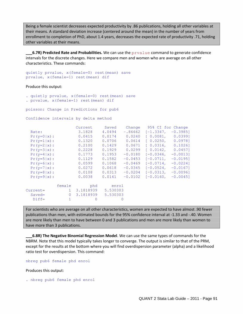
Being a female scientist decreases expected productivity by .86 publications, holding all other variables at their means. A standard deviation increase (centered around the mean) in the number of years from enrollment to completion of PhD, about 1.4 years, decreases the expected rate of productivity .71, holding other variables at their means. ___6.7R) Predicted Rate and Probabilities. We can use the prvalue command to generate confidence intervals for the discrete changes. Here we compare men and women who are average on all other characteristics. These commands: quietly prvalue, x(female=0) rest(mean) save prvalue, x(female=1) rest(mean) dif Produce this output: . quietly prvalue, x(female=0) rest(mean) save . prvalue, x(female=1) rest(mean) dif poisson: Change in Predictions for pub6 Confidence intervals by delta method Current Saved Change 95% CI for Change Rate: 3.1828 4.0494 -.86662 [-1.3347, -0.3985] Pr(y=0|x): 0.0415 0.0174 0.0240 [ 0.0081, 0.0399] Pr(y=1|x): 0.1320 0.0706 0.0614 [ 0.0250, 0.0978] Pr(y=2|x): 0.2100 0.1429 0.0671 [ 0.0316, 0.1026] Pr(y=3|x): 0.2228 0.1929 0.0299 [ 0.0142, 0.0457] Pr(y=4|x): 0.1773 0.1953 -0.0180 [-0.0346, -0.0013] Pr(y=5|x): 0.1129 0.1582 -0.0453 [-0.0711, -0.0195] Pr(y=6|x): 0.0599 0.1068 -0.0469 [-0.0714, -0.0224] Pr(y=7|x): 0.0272 0.0618 -0.0345 [-0.0524, -0.0167] Pr(y=8|x): 0.0108 0.0313 -0.0204 [-0.0313, -0.0096] Pr(y=9|x): 0.0038 0.0141 -0.0102 [-0.0160, -0.0045] female phd enrol Current= 1 3.1818939 5.530303 Saved= 0 3.1818939 5.530303 Diff= 1 0 0
For scientists who are average on all other characteristics, women are expected to have almost .90 fewer publications than men, with estimated bounds for the 95% confidence interval at ‐1.33 and ‐.40. Women are more likely than men to have between 0 and 3 publications and men are more likely than women to have more than 3 publications. ___6.8R) The Negative Binomial Regression Model. We can use the same types of commands for the NBRM. Note that this model typically takes longer to converge. The output is similar to that of the PRM, except for the results at the bottom where you will find overdispersion parameter (alpha) and a likelihood ratio test for overdispersion. This command: nbreg pub6 female phd enrol Produces this output: . nbreg pub6 female phd enrol

QUANT 2 Stata Lab Guide – 2011 - Page 92
Negative binomial regression Number of obs = 264 LR chi2(3) = 20.59 Dispersion = mean Prob > chi2 = 0.0001 Log likelihood = -642.723 Pseudo R2 = 0.0158 ------------------------------------------------------------------------------ pub6 | Coef. Std. Err. z P>|z| [95% Conf. Interval] -------------+---------------------------------------------------------------- female | -.2822292 .1382637 -2.04 0.041 -.553221 -.0112373 phd | .1995909 .0651859 3.06 0.002 .0718288 .327353 enrol | -.150895 .0480431 -3.14 0.002 -.2450578 -.0567322 _cons | 1.607418 .3379749 4.76 0.000 .9449989 2.269836 -------------+---------------------------------------------------------------- /lnalpha | -.203673 .1255831 -.4498113 .0424654 -------------+---------------------------------------------------------------- alpha | .8157291 .1024418 .6377485 1.04338 ------------------------------------------------------------------------------ Likelihood-ratio test of alpha=0: chibar2(01) = 394.12 Prob>=chibar2 = 0.000
Because there is significant evidence of overdispersion (G2=394.12, p< .001), the negative binomial regression model is preferred to the Poisson regression model. ___6.9R) ZIP Model. The zip command with the inf(indvars) option estimates a Zero‐Inflated Poisson Regression Model. You can “inflate” the same set of variables that are used in the PRM portion of the model or an entirely different set of variables. Here we “inflate” the variable phd. This command: zip pub6 female phd enrol, inf(phd) Produces this output: . zip pub6 female phd enrol, inf(phd) Zero-inflated Poisson regression Number of obs = 264 Nonzero obs = 212 Zero obs = 52 Inflation model = logit LR chi2(3) = 48.74 Log likelihood = -758.0032 Prob > chi2 = 0.0000 ------------------------------------------------------------------------------ | Coef. Std. Err. z P>|z| [95% Conf. Interval] -------------+---------------------------------------------------------------- pub6 | female | -.1210631 .0710846 -1.70 0.089 -.2603864 .0182602 phd | .1400257 .0334849 4.18 0.000 .0743964 .205655 enrol | -.1306837 .0250179 -5.22 0.000 -.1797178 -.0816496 _cons | 1.838966 .1749225 10.51 0.000 1.496124 2.181808 -------------+---------------------------------------------------------------- inflate | phd | -.2383082 .1657934 -1.44 0.151 -.5632572 .0866408 _cons | -.7539084 .5332584 -1.41 0.157 -1.799076 .291259 ------------------------------------------------------------------------------ ___6.10R) The ZINB Model. We can use the same types of commands for the ZINB. This command: zinb pub6 female phd enrol, inf(phd) Produces this output: . zinb pub6 female phd enrol, inf(phd)

QUANT 2 Stata Lab Guide – 2011 - Page 93
Zero-inflated negative binomial regression Number of obs = 264 Nonzero obs = 212 Zero obs = 52 Inflation model = logit LR chi2(3) = 18.91 Log likelihood = -642.2026 Prob > chi2 = 0.0003 ------------------------------------------------------------------------------ | Coef. Std. Err. z P>|z| [95% Conf. Interval] -------------+---------------------------------------------------------------- pub6 | female | -.2708994 .1371918 -1.97 0.048 -.5397905 -.0020084 phd | .1745669 .0695427 2.51 0.012 .0382657 .3108682 enrol | -.1527173 .047032 -3.25 0.001 -.2448984 -.0605362 _cons | 1.739814 .3498874 4.97 0.000 1.054047 2.42558 -------------+---------------------------------------------------------------- inflate | phd | -.5440498 .8665119 -0.63 0.530 -2.242382 1.154282 _cons | -1.456929 2.082817 -0.70 0.484 -5.539175 2.625316 -------------+---------------------------------------------------------------- /lnalpha | -.3514184 .2107589 -1.67 0.095 -.7644982 .0616614 -------------+---------------------------------------------------------------- alpha | .7036893 .1483088 .4655675 1.063602 ------------------------------------------------------------------------------ ___6.11R) Factor Change. Factor change coefficients can be computed after estimating the ZIP or ZINB models using listcoef. Since the output is similar, we show only the output for ZINB. The top half of the output, labeled Count Equation, contains coefficients for the factor change in the expected count for those in the Not Always Zero group. The bottom half, labeled Binary Equation, contains coefficients for the factor change in the odds of being in the Always Zero group compared with the Not Always Zero group. This command: listcoef, help Produces this output: . listcoef zinb (N=264): Factor Change in Expected Count Observed SD: 4.3102677 Count Equation: Factor Change in Expected Count for Those Not Always 0 ---------------------------------------------------------------------- pub6 | b z P>|z| e^b e^bStdX SDofX -------------+-------------------------------------------------------- female | -0.27090 -1.975 0.048 0.7627 0.8790 0.4762 phd | 0.17457 2.510 0.012 1.1907 1.1918 1.0052 enrol | -0.15272 -3.247 0.001 0.8584 0.8022 1.4432 -------------+-------------------------------------------------------- ln alpha | -0.35142 alpha | 0.70369 SE(alpha) = 0.14831 ---------------------------------------------------------------------- Binary Equation: Factor Change in Odds of Always 0 ---------------------------------------------------------------------- Always0 | b z P>|z| e^b e^bStdX SDofX -------------+-------------------------------------------------------- phd | -0.54405 -0.628 0.530 0.5804 0.5788 1.0052 ----------------------------------------------------------------------

QUANT 2 Stata Lab Guide – 2011 - Page 94
Among those who have the opportunity to publish, a standard deviation increase in PhD prestige increases the expected rate of publication by a factor of 1.2, holding other variables constant. A standard deviation increase in PhD prestige decreases the odds of not having the opportunity to publish by a factor of .58, although this is not significant (z=‐0.63, p=0.53). ___6.12R) Discrete and Marginal Changes. For the ZIP and ZINB models, prvalue produces two probabilities of zero counts: the probability of being zero and the probability of being always zero. This command: quietly prvalue , x(phd=1) rest(mean) save prvalue , x(phd=0) rest(mean) dif Produces this output: . quietly prvalue, x(phd=1) rest(mean) save . prvalue, x(phd=4) rest(mean) diff zinb: Change in Predictions for pub6 Current Saved Change Expected y: 4.3668 2.3388 2.0281 Pr(Always0|z): 0.0258 0.1191 -0.0933 Pr(y=0|x,z): 0.1545 0.3162 -0.1617 Pr(y=1|x): 0.1389 0.1824 -0.0435 Pr(y=2|x): 0.1277 0.1438 -0.0161 Pr(y=3|x): 0.1106 0.1068 0.0037 Pr(y=4|x): 0.0928 0.0769 0.0159 Pr(y=5|x): 0.0764 0.0543 0.0221 Pr(y=6|x): 0.0621 0.0379 0.0242 Pr(y=7|x): 0.0500 0.0261 0.0238 Pr(y=8|x): 0.0399 0.0179 0.0220 Pr(y=9|x): 0.0317 0.0122 0.0195 x values for count equation female phd enrol Current= .34469697 4 5.530303 Saved= .34469697 1 5.530303 Diff= 0 3 0 z values for binary equation phd Current= 4 Saved= 1 Diff= 3

QUANT 2 Stata Lab Guide – 2011 - Page 95
For an average scientist from a low prestige university, the probability of having no publications, either because the scientist does not have the opportunity to publish or because the scientist is a potential publisher who by chance did not publish, is .32. The probability of having no publications because the scientist does not have the opportunity to publish is .12. Thus most of the 0s for average scientists are due to being in the group who are “potential publishers.” We find that scientists from low prestige universities who are otherwise average are expected to have 2 fewer publications than scientists from high prestige universities who are otherwise average. ___6.13R) Compare model using countfit. countfit compares the fit of PRM, NBRM, ZIP, and ZINB, optionally generating a table of estimates, a table of differences between observed and average estimated probabilities, a graph of these differences, and various tests and measures of fit. This command: countfit pub6 female phd enrol, inf(female phd enrol) ///
graph(quant206a-count-rev-fig2.emf , replace) Produces this output: . countfit pub6 female phd enrol, inf(female phd enrol) /// > graph(quant206a-count-rev-fig2.emf , replace) . countfit pub6 female phd enrol, inf(phd) ---------------------------------------------------------------------------------- Variable | PRM NBRM ZIP ZINB ---------------------------------+------------------------------------------------ pub6 | Female: 1=female,0.. | 0.786 0.754 0.886 0.763 | -3.49 -2.04 -1.70 -1.97 Prestige of Ph.D. department. | 1.207 1.221 1.150 1.191 | 5.85 3.06 4.18 2.51 Years from BA to P.. | 0.876 0.860 0.877 0.858 | -5.51 -3.14 -5.22 -3.25 Constant | 4.630 4.990 6.290 5.696 | 9.02 4.76 10.51 4.97 ---------------------------------+------------------------------------------------ lnalpha | Constant | 0.816 0.704 | -1.62 -1.67 ---------------------------------+------------------------------------------------ inflate | Prestige of Ph.D. department. | 0.788 0.580 | -1.44 -0.63 Constant | 0.471 0.233 | -1.41 -0.70 ---------------------------------+------------------------------------------------ Statistics | alpha | 0.816 N | 264.000 264.000 264.000 264.000 ll | -839.781 -642.723 -758.003 -642.203 bic | 1701.865 1313.326 1549.462 1323.437 aic | 1687.561 1295.446 1528.006 1298.405 ---------------------------------------------------------------------------------- legend: b/t Comparison of Mean Observed and Predicted Count Maximum At Mean Model Difference Value |Diff| --------------------------------------------- PRM 0.163 0 0.051 NBRM 0.038 6 0.015 ZIP 0.100 1 0.033 ZINB 0.037 6 0.012

QUANT 2 Stata Lab Guide – 2011 - Page 96
PRM: Predicted and actual probabilities Count Actual Predicted |Diff| Pearson ------------------------------------------------ 0 0.197 0.034 0.163 205.490 1 0.144 0.100 0.044 4.992 2 0.129 0.161 0.032 1.688 3 0.121 0.185 0.064 5.777 4 0.095 0.170 0.075 8.815 5 0.053 0.133 0.080 12.712 6 0.091 0.092 0.001 0.003 7 0.023 0.057 0.035 5.546 8 0.042 0.033 0.009 0.589 9 0.023 0.018 0.005 0.371 ------------------------------------------------ Sum 0.917 0.983 0.507 245.982 NBRM: Predicted and actual probabilities Count Actual Predicted |Diff| Pearson ------------------------------------------------ 0 0.197 0.187 0.010 0.142 1 0.144 0.167 0.023 0.834 2 0.129 0.136 0.008 0.115 3 0.121 0.109 0.013 0.382 4 0.095 0.086 0.009 0.255 5 0.053 0.067 0.014 0.781 6 0.091 0.053 0.038 7.394 7 0.023 0.041 0.018 2.176 8 0.042 0.032 0.009 0.728 9 0.023 0.025 0.003 0.069 ------------------------------------------------ Sum 0.917 0.903 0.145 12.875 ZIP: Predicted and actual probabilities Count Actual Predicted |Diff| Pearson ------------------------------------------------ 0 0.197 0.197 0.000 0.000 1 0.144 0.044 0.100 59.264 2 0.129 0.088 0.041 4.940 3 0.121 0.124 0.003 0.016 4 0.095 0.137 0.042 3.465 5 0.053 0.127 0.074 11.353 6 0.091 0.102 0.011 0.320 7 0.023 0.073 0.050 9.169 8 0.042 0.048 0.006 0.193 9 0.023 0.028 0.006 0.306 ------------------------------------------------ Sum 0.917 0.969 0.332 89.027 ZINB: Predicted and actual probabilities Count Actual Predicted |Diff| Pearson ------------------------------------------------ 0 0.197 0.194 0.003 0.010 1 0.144 0.156 0.012 0.247 2 0.129 0.133 0.004 0.040 3 0.121 0.109 0.012 0.373

QUANT 2 Stata Lab Guide – 2011 - Page 97
4 0.095 0.087 0.008 0.179 5 0.053 0.069 0.016 0.958 6 0.091 0.054 0.037 6.598 7 0.023 0.042 0.020 2.416 8 0.042 0.033 0.008 0.567 9 0.023 0.026 0.003 0.109 ------------------------------------------------ Sum 0.917 0.904 0.123 11.496 Tests and Fit Statistics PRM BIC= 229.814 AIC= 6.392 Prefer Over Evidence ------------------------------------------------------------------------- vs NBRM BIC= -158.725 dif= 388.539 NBRM PRM Very strong AIC= 4.907 dif= 1.485 NBRM PRM LRX2= 394.115 prob= 0.000 NBRM PRM p=0.000 ------------------------------------------------------------------------- vs ZIP BIC= 84.385 dif= 145.429 ZIP PRM Very strong AIC= 5.787 dif= 0.605 ZIP PRM Vuong= 4.358 prob= 0.000 ZIP PRM p=0.000 ------------------------------------------------------------------------- vs ZINB BIC= -139.341 dif= 369.155 ZINB PRM Very strong AIC= 4.926 dif= 1.466 ZINB PRM ------------------------------------------------------------------------- NBRM BIC= -158.725 AIC= 4.907 Prefer Over Evidence ------------------------------------------------------------------------- vs ZIP BIC= 84.385 dif= -243.110 NBRM ZIP Very strong AIC= 5.787 dif= -0.880 NBRM ZIP ------------------------------------------------------------------------- vs ZINB BIC= -139.341 dif= -19.384 NBRM ZINB Very strong AIC= 4.926 dif= -0.019 NBRM ZINB Vuong= 0.834 prob= 0.202 ZINB NBRM p=0.202 ------------------------------------------------------------------------- ZIP BIC= 84.385 AIC= 5.787 Prefer Over Evidence ------------------------------------------------------------------------- vs ZINB BIC= -139.341 dif= 223.726 ZINB ZIP Very strong AIC= 4.926 dif= 0.861 ZINB ZIP LRX2= 229.302 prob= 0.000 ZINB ZIP p=0.000 -------------------------------------------------------------------------

QUANT 2 Stata Lab Guide – 2011 - Page 98
-.1-.0
50
.05
.1O
bser
ved-
Pre
dict
ed
0 1 2 3 4 5 6 7 8 9Count
PRM NBRMZIP ZINB
Note: positive deviations show underpredictions.
___6.14R) Close the Log File. log close exit

QUANT 2 Stata Lab Guide – 2011 - Page 99
Section 6: Models for Count Outcomes – EXERCISE The file quant206b-count-ex.do contains an outline of this exercise. ___6.1) Set‐up your do‐file. ___6.2) Load your data. ___6.3) Examine the data and select your variables. Choose one count dependent variable and at least
three independent variables (make sure one is binary and one is continuous). Drop cases with missing data and verify. Make sure to look at the distribution of your outcome variable.
___6.4) Estimate a NBRM. ___6.5) List the factor change coefficients using listcoef, help. Interpret a few of the
unstandardized and standardized factor change coefficients. ___6.6) Test NBRM against PRM and write up the results as though it were part of a research paper.
(Hint: use the LR test results at the end of the NBRM output) ___6.7) Use prvalue,save and prvalue,dif to calculate a discrete change. Interpret this. ___6.8) Estimate the same model using zip and zinb. ___6.9) List the factor change coefficients using listcoef, help for either the ZIP or ZINB model.
Interpret a few of the unstandardized and standardized factor change coefficients. ___6.10) Use prvalue,save and prvalue,dif to calculate a discrete change. Interpret this. ___6.11) Use countfit to compare count models. Which model do you prefer and why? ___6.12) Close log and exit do‐file.