appendix d air quality impact analysis methodology

APPENDIX D

AIR QUALITY IMPACT ANALYSIS METHODOLOGY

January 2007

D-3

APPENDIX D. AIR QUALITY IMPACT ANALYSIS METHODOLOGY

D.1 GENERAL APPROACH

The approach to assessing air quality impacts for a new or modified emission source generally begins by determining the impacts of the proposed facilities alone. If the impacts of the facilities are below specified significance impact levels, then no further analysis is required. The significant impact levels were previously presented in Table 4.1.1. If the impacts of proposed facilities are found to exceed a significant impact level, further analysis considering other existing sources and background pollutant concentrations is required for that significant impact level.

The approach used to analyze the potential impacts of the Stanton proposed IGCC facilities, as described in detail in the following subsections, was developed in accordance with accepted practice. Guidance contained in EPA manuals and user’s guides was sought and followed. In addition, a proposed modeling protocol was presented to the Florida Department of Environmental Protection for review and comment. Florida Department of Environmental Protection staff subsequently accepted this modeling protocol. The air quality analysis for the proposed IGCC facilities was conducted in accordance with the approved modeling protocol.

Attainment status of criteria pollutants is important information to be considered in the air quality impact analysis. As previously noted in Section 3.2.2, the entire state of Florida, including Orange County, is in attainment with NAAQS and state ambient air quality standards for all pollutants, including the recently implemented PM-2.5 and 8-hour O3 standards. The PSD Class I area nearest to the Stanton Energy Center is Chassahowitzka National Wildlife Refuge, about 90 miles to the west-northwest on the Gulf of Mexico.

D.2 POLLUTANTS EVALUATED Most emissions would result from combustion of synthesis gas in the gas combustion turbine during

normal operations. The exhaust gas would be released to the atmosphere via the 205-ft HRSG stack. Table 2.1.3 previously presented stack emissions at full load assuming pollutant removal by synthesis gas cleanup systems, but no post-combustion controls (i.e., no selective catalytic reduction or CO catalyst control). Annual emissions are conservatively based on continuous year-round operation (100% capacity factor). The principal pollutants would be SO2, NOx, particulate matter, CO, and volatile organic compounds (VOCs). Trace emissions of other pollutants would include formaldehyde, toluene, xylenes, carbon disulfide, acetaldehyde, mercury, beryllium, benzene, arsenic, and others (Table 2.1.3).

D.3 MODEL SELECTION AND USE Air quality models are applied at two levels: screening and refined. At the screening level, models

provide conservative estimates of impacts to determine whether more detailed modeling is required.

Orlando Gasification Project EIS

D-4

Screening modeling can also be used to identify worst-case operating scenarios for subsequent refined modeling analysis. The current version of EPA’s SCREEN3 Dispersion Model (EPA 1995a) (Version 96043; February 12, 1996) was employed as a screening tool to evaluate the various proposed IGCC/HRSG operating scenarios.

The refined level consists of techniques that provide more advanced technical treatment of atmospheric processes. Refined modeling requires more detailed and precise input data, but also provides improved estimates of source impacts. The American Meteorological Society (AMS)/EPA Regulatory MODel (AERMOD) modeling system (EPA 2004a; EPA 2004b) and 5 years of hourly meteorological data were used in the ambient impact analysis. AERMOD was used to obtain refined impact predictions for short-term periods (i.e., periods equal to or less than 24 hours). AERMOD was also utilized to obtain refined predictions of annual-average concentrations. D.3.1 Screening Model Techniques

The proposed IGCC facilities would operate under several operating scenarios. These scenarios include different loads and ambient air temperatures and the optional use of supplemental duct-burner-firing and inlet air evaporative cooling. Plume dispersion and, therefore, ground-level impacts, would be affected by these different operating scenarios since emission rates, exit temperatures, and exhaust gas velocities would change.

The SCREEN3 dispersion model was used to evaluate each IGCC HRSG operating scenario for each pollutant of concern to identify the scenarios that cause the highest impacts. The SCREEN3 model implements screening methods contained in EPA’s Screening Procedures for Estimating the Air Quality Impact of Stationary Sources, Revised. SCREEN3 is a simple model that calculates 1-hour average concentrations over a range of predefined worst-case meteorological conditions. The SCREEN3 model includes algorithms to assess building wake downwash effects and for analyzing concentrations in both simple and complex terrain.

A nominal emission rate of 10.0 grams per second (g/s) was used for all SCREEN3 model runs. The SCREEN3 model results were then adjusted to reflect the maximum emission rate for each operating scenario [i.e., model results were multiplied by the ratio of maximum emission rates (in g/s) to 10.0 g/s]. Summaries of the screening modeling results showing, for each IGCC HRSG operating scenario and pollutant evaluated, the SCREEN3 unadjusted 1-hour average maximum impact, emission rate adjustment ratio, and the adjusted SCREEN3 1-hour average maximum impact are provided in Section D.11.3. D.3.2 Refined Model Techniques

Regulatory agency recommended procedures for conducting air quality impact assessments are contained in EPA’s Guideline on Air Quality Models (GAQM). The GAQM is codified in Appendix W of 40 CFR 51. In the November 9, 2005, Federal Register, EPA approved the use of AERMOD as a GAQM Appendix A preferred model effective December 9, 2005. AERMOD is

January 2007

D-5

recommended for use in a wide range of regulatory applications, including both simple and complex terrain. The AERMOD modeling system consists of meteorological and terrain preprocessing programs (AERMET and AERMAP, respectively) and the AERMOD dispersion model. The latest version of AERMOD (Version 04300) was used to assess IGCC project air quality impacts at receptor locations within about 30 miles of the project site.

D.4 MODEL OPTIONS Procedures applicable to the AERMOD modeling system specified in the latest version of the

User’s Guide for the AMS/EPA Regulatory Model – AERMOD (September 2004) and EPA’s November 9, 2005, revisions to the GAQM were followed. In particular, the AERMOD control pathway MODELOPT keyword parameters DFAULT and CONC were selected. Selection of the parameter DFAULT, which specifies use of the regulatory default options, is recommended by the GAQM. The CONC option specifies the calculation of concentrations. The proposed IGCC facilities would be located in southeastern Orange County. AERMOD options pertinent to urban areas, including increased surface heating (URBANOPT keyword) and pollutant exponential decay (HALFLIFE and DCAYCOEF keywords) were not employed. In addition, the option to use flagpole receptors (FLAGPOLE keyword) was not selected.

The AERMOD modeling system was used to determine short-term and annual average impact predictions by using the PERIOD parameter for the AVERTIME keyword.

D.5 NO2 AMBIENT IMPACT ANALYSIS For annual NO2 impacts, the tiered screening approach described in the GAQM, was used. Tier 1

of this screening procedure assumes complete conversion of NOx to NO2. Tier 2 applies an empirically derived NO2/NOx ratio of 0.75 to the Tier 1 results.

D.6 TERRAIN CONSIDERATION The GAQM defines flat terrain as terrain equal to the elevation of the stack base, simple terrain as

terrain lower than the height of the stack top, and complex terrain as terrain exceeding the height of the stack being modeled.

Site elevation for the Stanton Energy Center is approximately 70 ft above mean sea level (ft-msl). The proposed IGCC HRSG stack height would be at an elevation of 205 ft above grade. Accordingly, terrain elevations above approximately 275 ft-msl would be classified as complex terrain. U.S. Geological Survey (USGS) 7.5-minute series topographic maps were examined for terrain features in the IGCC impact area (i.e., within an approximate 9-mile radius). Based on this examination, terrain in the vicinity of the site is classified as either flat or simple terrain.

In accordance with the GAQM recommendations for AERMOD, each modeled receptor was assigned a terrain elevation based on USGS 7.5-minute digital elevation model data and use of the AERMAP (Version 04300) preprocessing program. AERMAP was utilized in accordance with the


D-6

latest version (December 2005) of the user’s guide for the AERMOD terrain preprocessor (AERMAP) and EPA’s November 9, 2005, revisions to the GAQM. AERMAP prepares terrain data for use by AERMOD in simple and complex terrain situations. This allows AERMOD to account for terrain using a simplification of the procedure used in the CTDMPLUS air dispersion model.

D.7 BUILDING WAKE EFFECTS The Clean Air Act Amendments of 1990 require the degree of emission limitation for control of

any pollutant to not be affected by a stack height that exceeds good engineering practice (GEP) or any other dispersion technique. On July 8, 1985, EPA promulgated final stack height regulations (40 CFR 51). GEP stack height is defined as the highest of 65 meters, or a height established by applying the formula: Hg = H + 1.5 L where: Hg = GEP stack height. H = height of the structure or nearby structure. L = lesser dimension (height or projected width) of the nearby structure.

Nearby is defined as a distance up to five times the lesser of the height or width dimension of a structure or terrain feature, but not greater than 800 m. While GEP stack height regulations require that stack height used in modeling for determining compliance with NAAQS and PSD increments not exceed the GEP stack height, the actual stack height may be greater. Guidelines for determining GEP stack height have been issued by EPA (1985b).

The height proposed for the Stanton IGCC HRSG stack (i.e., 205 ft above grade level), as well as all other project emission sources, would be less than the de minimis GEP height of 65 meters (213 ft). Since the stack heights of the IGCC project emission sources would comply with the EPA promulgated final stack height regulations (40 CFR 51), actual project stack heights were used in the modeling analyses.

While the GEP stack height rules address the maximum stack height that can be employed in a dispersion model analysis, stacks having heights lower than GEP stack height can potentially result in higher downwind concentrations due to building downwash effects. AERMOD evaluates the effects of building downwash based on the plume rise model enhancements (PRIME) building downwash algorithms. For the IGCC ambient impact analysis, the complex downwash analysis implemented by AERMOD was performed using the current version of EPA’s Building Profile Input Program (BPIP) for PRIME (BPIPPRM) (Version 04274; September 30, 2004). The EPA BPIP program was used to determine the area of influence for each building, whether a particular stack is subject to building downwash, the area of influence for directionally dependent building downwash, and finally to generate the specific building dimension data required by the model. BPIP output consists of an array

January 2007

D-7

of 36 direction-specific (10° to 360°) building heights (BUILDHGT keyword), lengths (BUILDLEN keyword), widths (BUILDWID keyword), and along-flow (XBADJ keyword) and across-flow (YBADJ keyword) distances for each stack suitable for use as input to AERMOD. Dimensions of the building/structures evaluated for the wake effects were determined from engineering layouts and specifications and are shown in Table D.1. The buildings are shown as three-dimensional projections in Figure D.1.

Table D.1. Building/structure dimensions

Dimensions Building/Structure

Width

(m) Length

(m) Height

(m)

Natural gas unit steam turbine 18.3 43.2 13.5

Natural gas unit cooling tower 38.2 83.0 18.1

Natural gas unit 1A HRSG 12.1 47.5 25.6

Natural gas unit 2A HRSG 12.1 47.5 25.6

Natural gas unit administration building 18.3 33.2 5.3

Proposed IGCC HRSG 11.7 38.2 34.8

Proposed IGCC combustion turbine 10.3 28.7 9.7

Proposed IGCC fan inlet 9.4 18.0 21.3

Proposed IGCC gasifier structure 53.5 73.2 53.1

Proposed IGCC cooling tower 37.0 50.8 15.0

Proposed IGCC steam turbine 14.2 36.5 9.7

Proposed IGCC control building 18.5 33.2 5.1

Unit 1 cooling tower — 93.5 (diameter) 131.4

Unit 1 boiler 55.6 78.5 68.6

Unit 2 cooling tower — 93.5 (diameter) 131.4

Unit 2 boiler 51.7 80.8 68.6

Unit 2 precipitator 37.4 56.8 33.5

Air quality control building for Unit 2 54.3 67.2 32.0

Steam turbines for Units 1 and 2 32.4 158.0 30.5

Coal storage pile 91.4 121.9 10.7 Source: OUC 2006.


D-8

Figure D.1. Buildings used in the downwash analysis

The entire perimeter of the Stanton Energy Center is fenced. Therefore, the nearest locations of

general public access are at the facility fence lines.

Consistent with GAQM and Florida Department of Environmental Protection recommendations, the ambient impact analysis used the following receptor grids:

• Fence line receptors—Receptors placed on the site fence line spaced 164-ft apart.

• Near-Field Cartesian Receptors—Receptors between the center of the site and extending out to approximately 2 miles at 328-ft spacings.

• Mid-Field Cartesian Receptors—Receptors between about 2 miles and extending to approximately 4 miles at 820-ft spacings.

• Far-Field Cartesian Receptors—Receptors between about 4 miles and extending to approximately 9 miles at 1,640-ft spacings.

January 2007

D-9

Figure D.2 illustrates a graphical representation of the near-field receptor grids (out to a distance of about 2 miles). A depiction of the full receptor grid (from about 2 to 9 miles) is shown in Figure D.3.

Figure D.2. Near-field receptor grid


D-10

Figure D.3. Full receptor grid

January 2007

D-11

D.9 METEOROLOGICAL DATA The AERMOD meteorological preprocessor AERMET (Version 04300) was used to process

surface meteorological data collected at the Orlando International Airport (OIA) (Weather Bureau, Air Force and Navy Station No. 12815) and upper air data from Tampa Bay/Ruskin (Station No. 92801). Raw surface and upper air data for the years 1996 to 2000 were obtained from the National Climatic Data Center. Missing surface and upper air data (i.e., data gaps) were filled in accordance with EPA guidance.

AERMET creates two files that are used by AERMOD (i.e., surface and profile files). The surface file contains boundary layer parameters including friction velocity, Monin-Obukhov length, convective velocity scale, temperature scale, convectively generated boundary layer height, stable boundary layer height, and surface heat flux. The profile file contains multilevel data of wind speed, wind direction, and temperature. AERMET was utilized in accordance with the latest version (February 2005) of the User’s Guide for the AERMOD Meteorological Preprocessor (AERMET) and EPA’s November 9, 2005, revisions to the GAQM.

AERMET calculates hourly boundary layer parameters for use by AERMOD, including friction velocity, Monin-Obukhov length, convective velocity scale, temperature scale, convectively generated boundary layer height, stable boundary layer height, and surface heat flux. In addition, AERMET passes all observed meteorological parameters to AERMOD including wind direction and speed (at multiple heights, if available), temperature, and if available, measured turbulence. AERMOD uses this information to calculate concentrations in a manner that accounts for a dispersion rate that is a continuous function of meteorology. D.9.1 Selection of Surface Characteristics

The AERMET preprocessing program was used to develop the meteorological data required by AERMOD. Area characteristics in the vicinity of proposed emission sources are important in determining the boundary layer parameter estimates. Obstacles to the wind flow, amount of moisture at the surface, and reflectivity of the surface all affect the boundary layer parameter estimates. The AERMET keywords FREQ_SECT, SECTOR, and SITE_CHAR are used to define the surface albedo, Bowen ratio, and surface roughness length (zo). Figure D.4 shows the land use in the vicinity of the site that was used to determine the area characteristics.

The albedo is the fraction of total incident solar radiation reflected by the surface back to space without absorption. The daytime Bowen ratio is an indicator of surface moisture and is used for determining planetary boundary layer parameters for convective conditions. The surface roughness length is related to the height of obstacles to the wind flow and represents the height at which the mean horizontal wind speed is zero.

Guidance contained in the AERMET User’s Guide (Tables 4-1 through 4-3), in conjunction with vicinity land use and aerial maps, were used to define the seasonal values of surface albedo, daytime


D-12

Figure D.4. Existing land use on Stanton site and surroundings as of 2000

January 2007

D-13

Bowen ratio, and surface roughness length for the proposed IGCC air quality impact assessment. The following specific AERMET parameters were used:

• After examining upwind fetch distances of about 2 miles, five sectors were defined for site characteristics. More than 80% of the land use in this area was found to be rural containing swamp (wetlands) and cultivated land use types provided in the AERMET User’s Guide.

• Surface characteristics such as albedo, Bowen ratio, and surface roughness were assumed to vary seasonally, and parameters appropriate for the defined land use types were taken from the AERMET User’s Guide.

D.10 MODELED EMISSION INVENTORY In addition to the combined-cycle unit (the primary proposed emission source), the proposed

IGCC facilities would include coal receiving, storage, handling, and feed preparation fugitive and point sources of PM/PM-10, a flare (for combustion of synthesis gas during startups and plant upsets), and a mechanical draft cooling tower.

Because proposed IGCC maximum air quality impacts were below the significant impact levels for all PSD pollutants, a full, multi-source interactive assessment of NAAQS attainment and PSD Class II increment consumption was not required.

D.11 AMBIENT IMPACT ANALYSIS RESULTS

D.11.1 Overview Comprehensive screening and refined modeling was conducted to assess the air quality impacts

resulting from proposed IGCC operations in accordance with the Florida Department of Environmental Protection-approved modeling protocol. This section provides the results of the air quality assessment with respect to near-field impacts (i.e., at receptors located within about 30 miles of the project site). D.11.2 Conclusions

Comprehensive dispersion modeling using the EPA SCREEN3 (screening) and AERMOD (refined) dispersion models demonstrates that operation of the proposed IGCC facilities would result in ambient air quality impacts that would be well below the significant impact levels for all pollutants and all averaging periods. Accordingly, a multi-source interactive assessment of air quality impacts with respect to the ambient air quality standards and PSD Class II increments was not required.

Assessment of proposed IGCC toxic air pollutant emissions demonstrates that all project ambient air quality impacts for air toxics would be well below the relevant EPA-recommended exposure criteria.


D-14

D.11.3 Screening Modeling Results As previously described, the EPA SCREEN3 dispersion model was used to assess each of the

proposed IGCC HRSG operating cases. To aid in assessing the screening results, the operating cases were logically divided into two groups consistent with the emission calculations. Specifically, synthesis gas and natural gas firing operations each have a set of operating conditions defined by combustion turbine load, combustion turbine inlet air evaporative cooling, and HRSG duct burner firing. The combustion turbine HRSG operating cases evaluated for the air quality analyses include combinations of load (i.e., 100, 75, and 50%), ambient temperature (20, 70, and 95°F), and optional use of combustion turbine inlet air evaporative cooling and HRSG duct burner firing. The specific stack parameters (i.e., stack height, diameter, exhaust gas temperature, and velocity) associated with each operating case were previously shown.

The specific exhaust gas temperatures and velocities for each operating case were employed in SCREEN3. Since SCREEN3 model results are directly proportional to emission rates, an emission rate of 10.0 g/sec was used for all IGCC HRSG operating cases so that the model results could be easily scaled to reflect the specific emission rates for each modeled pollutant. Modeling was conducted for the IGCC pollutants that would be projected to exceed the PSD significant emission rate thresholds as previously shown (i.e., NOx, SO2, PM-10, and CO).

The SCREEN3 model results were used to identify the specific IGCC HRSG operational cases that would be expected to produce the highest air quality impacts. These worst-case operating cases for each pollutant were then carried forward to the refined modeling analyses.

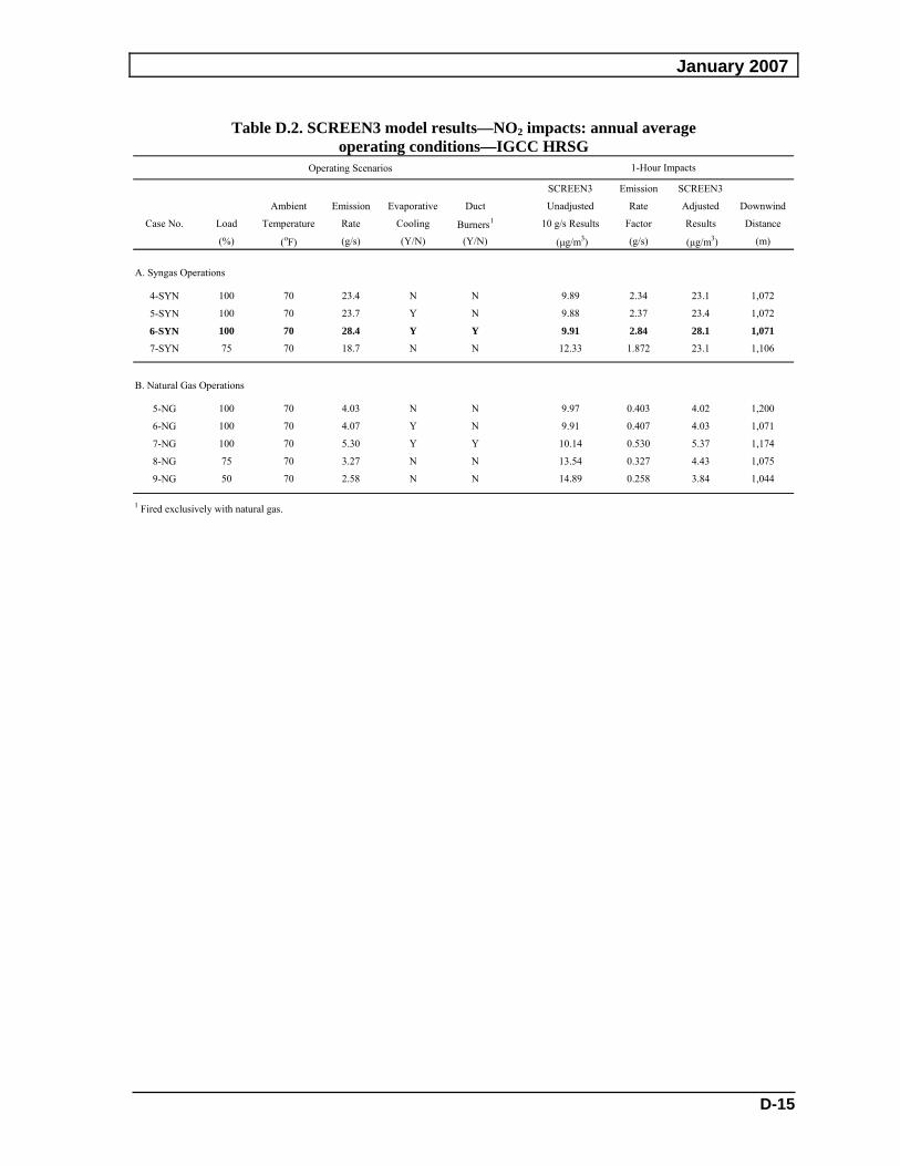
SCREEN3 model results for NO2, SO2, PM-10, and CO while firing synthesis gas and natural gas are shown in Tables D.2 through D.5, respectively. For each of these pollutants, the synthesis gas operating cases resulted in higher impacts than the natural gas cases.

For NO2, Table D.2 shows that Case No. 6-Syn (100% load at 70ºF, duct firing, and evaporative cooling) results in the highest predicted hourly average concentration of 28.1 µg/m3. Therefore, Case No. 6-Syn was selected for the refined NO2 analyses.

For SO2, Table D.3 shows that Case No. 10-Syn (100% load at 95ºF, duct firing, and evaporative cooling) results in the highest predicted hourly average concentration of 5.41 µg/m3. Therefore, Case No. 10-Syn was selected for the refined SO2 analyses.

For PM-10, Table D.4 shows that Case No. 10-Syn (100% load at 95ºF, duct firing, and evaporative cooling) results in the highest predicted hourly average concentration of 5.48 µg/m3. Therefore, Case No. 10-Syn was selected for the remainder of the PM-10 analyses.

For CO, Table D.5 shows that Case No. 10-Syn (100% load at 95ºF, duct firing, and evaporative cooling) results in the highest predicted hourly average concentration of 22.29 µg/m3. Therefore, Case No. 10-Syn was selected for the remainder of the CO analyses.

January 2007

D-15

Table D.2. SCREEN3 model results—NO2 impacts: annual average operating conditions—IGCC HRSG

Operating Scenarios

SCREEN3 Emission SCREEN3

Ambient Emission Evaporative Duct Unadjusted Rate Adjusted Downwind

Case No. Load Temperature Rate Cooling Burners1 10 g/s Results Factor Results Distance

(%) ( oF) (g/s) (Y/N) (Y/N) (μg/m3) (g/s) (μg/m 3 ) (m)

A. Syngas Operations 4-SYN 100 70 23.4 N N 9.89 2.34 23.1 1,072

5-SYN 100 70 23.7 Y N 9.88 2.37 23.4 1,072

6-SYN 100 70 28.4 Y Y 9.91 2.84 28.1 1,071

7-SYN 75 70 18.7 N N 12.33 1.872 23.1 1,106

B. Natural Gas Operations 5-NG 100 70 4.03 N N 9.97 0.403 4.02 1,200

6-NG 100 70 4.07 Y N 9.91 0.407 4.03 1,071

7-NG 100 70 5.30 Y Y 10.14 0.530 5.37 1,174

8-NG 75 70 3.27 N N 13.54 0.327 4.43 1,075

9-NG 50 70 2.58 N N 14.89 0.258 3.84 1,044

1 Fired exclusively with natural gas.

1-Hour Impacts


D-16

Table D.3. SCREEN3 model results—SO2 impacts— IGCC HRSG Operating Scenarios




(%) (oF) (g/s) (Y/N) (Y/N) (µg/m3) (g/s) (µg/m3) (m)

A. Syngas Operations

1-SYN 100 20 4.51 N N 8.60 0.451 3.88 1,1152-SYN 100 20 4.55 N Y 8.70 0.455 3.96 1,1103-SYN 75 20 3.67 N N 9.79 0.367 3.59 1,0744-SYN 100 70 4.41 N N 9.89 0.441 4.36 1,0725-SYN 100 70 4.48 Y N 9.88 0.448 4.42 1,0726-SYN 100 70 4.52 Y Y 9.91 0.452 4.48 1,0717-SYN 75 70 3.57 N N 12.3 0.357 4.40 1,1068-SYN 100 95 3.97 N N 13.2 0.397 5.22 1,0859-SYN 100 95 4.27 Y N 12.2 0.427 5.20 1,110

10-SYN 100 95 4.31 Y Y 12.6 0.431 5.41 1,10011-SYN 75 95 3.27 N N 16.1 0.327 5.26 1,019

B. Natural Gas Operations1-NG 100 20 0.146 N N 7.79 0.0146 0.114 1,1482-NG 100 20 0.182 N Y 8.06 0.0182 0.147 1,1363-NG 75 20 0.118 N N 9.79 0.0118 0.115 1,0744-NG 50 20 0.091 N N 9.92 0.0091 0.090 1,0715-NG 100 70 0.131 N N 9.97 0.0131 0.131 1,2006-NG 100 70 0.132 N N 9.91 0.0132 0.131 1,0717-NG 100 70 0.172 N Y 10.1 0.0172 0.174 1,1748-NG 75 70 0.106 N N 13.5 0.0106 0.144 1,0759-NG 50 70 0.084 N N 14.9 0.0084 0.125 1,04410-NG 100 95 0.121 N N 13.4 0.0121 0.162 1,07811-NG 100 95 0.127 N N 12.8 0.0127 0.163 1,09312-NG 100 95 0.165 N Y 13.2 0.0165 0.218 1,08213-NG 75 95 0.101 N N 17.0 0.0101 0.172 1,00214-NG 50 95 0.079 N N 19.4 0.0079 0.153 962


1-Hour Impacts

January 2007

D-17

Table D.4. SCREEN3 model results—PM-10 impacts—IGCC HRSG Operating Scenarios





A. Syngas Operations2-SYN 100 20 4.57 N Y 8.70 0.457 3.98 1,1103-SYN 75 20 3.18 N N 9.79 0.318 3.11 1,0744-SYN 100 70 3.83 N N 9.89 0.383 3.79 1,0725-SYN 100 70 3.88 Y N 9.88 0.388 3.83 1,0726-SYN 100 70 4.51 Y Y 9.91 0.451 4.47 1,0717-SYN 75 70 3.10 N N 12.3 0.310 3.82 1,1068-SYN 100 95 3.44 N N 13.2 0.344 4.52 1,0859-SYN 100 95 3.70 Y N 12.2 0.370 4.51 1,110

10-SYN 100 95 4.37 Y Y 12.6 0.437 5.48 1,10011-SYN 75 95 2.83 N N 16.1 0.283 4.56 1,019



1-Hour Impacts

Source: OUC 2006.


D-18

Table D.5. SCREEN3 model results for CO impacts—IGCC HRSG Operating Scenarios





A. Syngas Operations

1-SYN 100 20 11.31 N N 8.60 1.131 9.72 1,1152-SYN 100 20 18.04 N Y 8.70 1.804 15.70 1,1103-SYN 75 20 9.25 N N 9.79 0.925 9.06 1,0744-SYN 100 70 11.33 N N 9.89 1.133 11.20 1,0725-SYN 100 70 11.42 Y N 9.88 1.142 11.28 1,0726-SYN 100 70 17.70 Y Y 9.91 1.770 17.53 1,0717-SYN 75 70 9.18 N N 12.3 0.918 11.32 1,1068-SYN 100 95 10.45 N N 13.2 1.045 13.74 1,0859-SYN 100 95 11.06 Y N 12.2 1.106 13.47 1,110

10-SYN 100 95 17.76 Y Y 12.6 1.776 22.29 1,10011-SYN 75 95 8.78 N N 16.1 0.878 14.14 1,019



1-Hour Impacts

January 2007

D-19

D.11.4 REFINED MODELING RESULTS The refined EPA AERMOD modeling system, using five years (1996–2000) of hour-by-hour

meteorology and comprehensive receptor grids, was employed to evaluate each of the maximum impact operating cases identified by the SCREEN3 model.

Detailed proposed IGCC AERMOD results for each year of meteorology are summarized in Table D.6 (annual NO2), Table D.7 (annual SO2), Table D.8 (24-hour SO2), Table D.9 (3-hour SO2), Table D.10 (annual PM-10), Table D.11 (24-hour PM-10), Table D.12 (8-hour CO), and Table D.13 (1-hour CO). These tables provide maximum IGCC impacts, the locations of these impacts, and relevant regulatory criteria.

Maximum IGCC air quality impacts using AERMOD and the identified worst-case operating cases are summarized in Table D.14. The AERMOD results presented in Table D.14 demonstrate that IGCC air quality impacts, for all pollutants and averaging periods, would be below the significant impact levels (also see Table 4.1.1). D.11.5 AIR TOXICS MODELING RESULTS

The refined AERMOD modeling system was also used to assess IGCC impacts with respect to toxic air pollutants. Tables D.15 and D.16 show (for synthesis gas and natural gas, respectively) maximum IGCC air quality impacts for a variety of metallic and organic toxic air pollutants in comparison to chronic and acute exposure criteria obtained from EPA’s Integrated Risk Information System (IRIS). As shown in Tables D.15 and 16, all IGCC ambient impacts with respect to air toxics are below the EPA-recommended exposure criteria.


D-20

Table D.6. AERMOD model results—maximum annual average NO2 impacts

Maximum Annual Impacts 1996 1997 1998 1999 2000

Unadjusted AERMOD Impact (µg/m3)1 0.0273 0.0269 0.0277 0.0207 0.0214 Unit B CT/HRSG Emission Rate (g/s) 28.40 28.40 28.40 28.40 28.40 Tier 1 Impact (µg/m3)2 0.776 0.763 0.787 0.588 0.608 Tier 2 Impact (µg/m3)3 0.582 0.573 0.590 0.441 0.456 PSD Significant Impact (µg/m3) 1.0 1.0 1.0 1.0 1.0 Exceed PSD Significant Impact (Y/N) N N N N NPercent of PSD Significant Impact (%) 58.2 57.3 59.0 44.1 45.6 PSD de minimis Ambient Impact Threshold (µg/m3) 14.0 14.0 14.0 14.0 14.0 Exceed PSD de minimis Ambient Impact (Y/N) N N N N NReceptor UTM Easting (m) 483,577 483,676 483,676 483,725 483,775 Receptor UTM Northing (m) 3,151,975 3,151,976 3,151,976 3,151,976 3,151,976 Distance From Grid Origin (m) 1,026 1,027 1,027 1,031 1,038 Direction From Grid Origin (Vector o) 358 3 3 6 9

1 Based on modeled emission rate of 1.0 g/s.2 Unadjusted AERMOD impact times Unit B CT/HRSG emission rate (assumed complete conversion of NOx to NO2; i.e., NO2/NOx ratio of 1.0).3 Tier 1 impact times USEPA national default NO2/NOx ratio of 0.75.

Table D.7. AERMOD model results—maximum annual average SO2 impacts


Unadjusted AERMOD Impact (µg/m3)1 0.0278 0.0274 0.0281 0.0210 0.0215 Unit B CT/HRSG Emission Rate (g/s) 4.31 4.31 4.31 4.31 4.31 Adjusted Impact (µg/m3)2 0.120 0.118 0.121 0.091 0.092 PSD Significant Impact (µg/m3) 1.0 1.0 1.0 1.0 1.0 Exceed PSD Significant Impact (Y/N) N N N N NPercent of PSD Significant Impact (%) 12.0 11.8 12.1 9.1 9.2 Receptor UTM Easting (m) 483,577 483,676 483,676 483,725 483,824 Receptor UTM Northing (m) 3,151,975 3,151,976 3,151,976 3,151,976 3,151,976 Distance From Grid Origin (m) 1,026 1,027 1,027 1,031 1,046 Direction From Grid Origin (Vector o) 358 3 3 6 11

1 Based on modeled emission rate of 1.0 g/s.2 Unadjusted AERMOD impact times Unit B CT/HRSG emission rate.

January 2007

D-21

Table D.8. AERMOD model results—maximum 3-hour average SO2 impacts

Maximum 3-Hour Impacts 1996 1997 1998 1999 2000

Unadjusted AERMOD Impact (µg/m3)1 0.567 0.700 0.710 0.486 0.506 Unit B CT/HRSG Emission Rate (g/s) 4.31 4.31 4.31 4.31 4.31 Adjusted Impact (µg/m3)2 2.44 3.02 3.06 2.09 2.18 PSD Significant Impact (µg/m3) 25.0 25.0 25.0 25.0 25.0 Exceed PSD Significant Impact (Y/N) N N N N NPercent of PSD Significant Impact (%) 9.8 12.1 12.2 8.4 8.7 Receptor UTM Easting (m) 484,567 483,626 483,626 483,676 482,686 Receptor UTM Northing (m) 3,151,979 3,151,975 3,151,975 3,151,976 3,151,971 Distance From Grid Origin (m) 1,399 1,025 1,025 1,027 1,384 Direction From Grid Origin (Vector o) 43 0 0 3 318 Date of Maximum Impact 1/2/96 4/28/97 1/27/98 1/02/99 11/24/00Julian Date of Maximum Impact 02 118 27 02 329Ending Hour of Maximum Impact 2100 0300 0600 2100 2400


Table D.9. AERMOD model results—maximum 24-hour average SO2 impacts


Unadjusted AERMOD Impact (µg/m3)1 0.241 0.273 0.328 0.250 0.200 Unit B CT/HRSG Emission Rate (g/s) 4.31 4.31 4.31 4.31 4.31 Adjusted Impact (µg/m3)2 1.04 1.18 1.41 1.08 0.86 PSD Significant Impact (µg/m3) 5.0 5.0 5.0 5.0 5.0 Exceed PSD Significant Impact (Y/N) N N N N NPercent of PSD Significant Impact (%) 20.8 23.5 28.2 21.6 17.2 PSD de minimis Ambient Impact Threshold (µg/m3) 13.0 13.0 13.0 13.0 13.0 Exceed PSD de minimis Ambient Impact (Y/N) N N N N NPercent of PSD de minimis Ambient Impact (%) 8.0 9.0 10.9 8.3 6.6 Receptor UTM Easting (m) 483,577 483,725 483,478 483,478 482,636 Receptor UTM Northing (m) 3,151,975 3,151,976 3,151,975 3,151,975 3,151,971 Distance From Grid Origin (m) 1,026 1,031 1,034 1,034 1,418 Direction From Grid Origin (Vector o) 358 6 352 352 316 Date of Maximum Impact 10/07/96 04/28/97 03/08/98 01/23/99 11/24/00Julian Date of Maximum Impact 281 118 67 23 329


Table D.10. AERMOD model results—maximum annual average PM-10 impacts


AERMOD Impact (µg/m3)1 0.3075 0.3463 0.3331 0.2763 0.2502 PSD Significant Impact (µg/m3) 1.0 1.0 1.0 1.0 1.0 Exceed PSD Significant Impact (Y/N) N N N N NPercent of PSD Significant Impact (%) 30.7 34.6 33.3 27.6 25.0 Receptor UTM Easting (m) 483,527 483,577 483,577 483,181 483,577 Receptor UTM Northing (m) 3,151,975 3,151,975 3,151,975 3,151,973 3,151,975 Distance From Grid Origin (m) 1,029 1,026 1,026 1,114 1,026 Direction From Grid Origin (Vector o) 355 358 358 337 358

1 Impact for all Unit B PM10 emission sourcers.

D-22

Orlando G

asification Project EIS

Table D.11. AERMOD model results—maximum 24-hour average PM-10 impacts


AERMOD Impact (µg/m3)1 2.748 4.381 3.067 3.862 3.412 PSD Significant Impact (µg/m3) 5.0 5.0 5.0 5.0 5.0 Exceed PSD Significant Impact (Y/ N N N N NPercent of PSD Significant Impact (%) 55.0 87.6 61.3 77.2 68.2 PSD de minimis Ambient Impact Threshold (µg/m3) 10.0 10.0 10.0 10.0 10.0 Exceed PSD de minimis Ambient Impact (Y/N ) N N N N NReceptor UTM Easting (m) 483,500 483,577 484,022 483,600 483,428 Receptor UTM Northing (m) 3,148,706 3,151,975 3,151,977 3,152,050 3,151,974 Distance From Grid Origin (m) 2,247 1,026 1,103 1,100 1,042 Direction From Grid Origin (Vector o) 183 358 21 359 349 Date of Maximum Impac 12/31/96 01/04/97 09/21/98 06/16/99 07/26/00Julian Date of Maximum Impact 366 04 264 167 208

1 Impact for all Unit B PM10 emission sourcers.

D-23

January 2007


D-24

Table D.12. AERMOD model results—maximum 8-hour

average CO impacts


Unadjusted AERMOD Impact (µg/m3)1 0.460 0.573 0.539 0.393 0.393 Unit B CT/HRSG Emission Rate (g/s) 17.8 17.8 17.8 17.8 17.8 Adjusted Impact (µg/m3)2 8.17 10.2 9.57 6.98 6.98 PSD Significant Impact (µg/m3) 500.0 500.0 500.0 500.0 500.0 Exceed PSD Significant Impact (Y/N) N N N N NPercent of PSD Significant Impact (%) 1.6 2.0 1.9 1.4 1.4 PSD de minimis Ambient Impact Threshold (µg/m3) 575.0 575.0 575.0 575.0 575.0 Exceed PSD de minimis Ambient Impact (Y/N) N N N N NPercent of PSD de minimis Ambient Impact (%) 1.4 1.8 1.7 1.2 1.2 Receptor UTM Easting (m) 483,626 483,676 482,933 483,478 483,923 Receptor UTM Northing (m) 3,151,975 3,151,976 3,151,972 3,151,975 3,151,977 Distance From Grid Origin (m) 1,025 1,027 1,232 1,034 1,071 Direction From Grid Origin (Vector o) 0 3 326 352 16 Date of Maximum Impact 04/30/96 04/28/97 02/16/98 02/01/99 01/23/00Julian Date of Maximum Impact 121 118 47 32 23Ending Hour of Maximum Impact 0800 0800 0800 1600 1600


Table D.13. AERMOD model results—maximum 1-hour average CO impacts


Unadjusted AERMOD Impact (µg/m3)1 0.768 0.763 0.772 0.741 0.747 Unit B CT/HRSG Emission Rate (g/s) 17.8 17.8 17.8 17.8 17.8 Adjusted Impact (µg/m3)2 13.6 13.6 13.7 13.2 13.3 PSD Significant Impact (µg/m3) 2,000.0 2,000.0 2,000.0 2,000.0 2,000.0 Exceed PSD Significant Impact (Y/N) N N N N NPercent of PSD Significant Impact (%) 0.7 0.7 0.7 0.7 0.7 Receptor UTM Easting (m) 483,626 483,725 483,626 483,626 483,577 Receptor UTM Northing (m) 3,151,975 3,151,976 3,151,975 3,151,975 3,151,975 Distance From Grid Origin (m) 1,025 1,031 1,025 1,025 1,026 Direction From Grid Origin (Vector o) 0 6 0 0 358 Date of Maximum Impact 06/11/96 09/27/97 09/03/98 12/12/99 04/13/00Julian Date of Maximum Impac 163 270 246 346 104Ending Hour of Maximum Impact 2000 0100 0500 0800 1900


January 2007

D-25

Table D.14. Refined (AERMOD) modeling results— maximum criteria pollutant impacts

Pollutant

Averaging

time Maximum impact

(µg/m3)

Significant impact level

(µg/m3)

NO2 Annual 0.59 1

PM-10 Annual 0.35 1 24-hour 4.4 5

SO2 Annual 0.12 1 24-hour 1.4 5 3-hour 3.1 25

CO 8-Hour 10.2 500 1-Hour 13.7 2,000

Source: OUC 2006.


D-26

Table D.15. Refined (AERMOD) model results—toxic air pollutants; synthesis gas SHORT-TERM RISK LONG-TERM RISK

Maximum Acute Inhalation

CT/HRSG 1-hr Aver-

age Inhalation Percent of Unit Risk Reference Emissionsa Impactb Exposurec Exposure Factord Concentrationd Cancer Hazard

Chemical Compound (g/s) (µg/m3) (µg/m3) Limit (µg/m3)-1 (µg/m3) Riske Coefficientf

2-Methylnaphthalene 1.08E-04 8.35E-05 6.00E+03 0.000001% NA NA NA NA

Acenaphthyalene 7.81E-06 6.03E-06 2.00E+03 0.0000003% NA NA NA NA

Acetaldehyde 5.41E-04 4.18E-04 1.80E+04 0.000002% 2.20E-06 9.00E+00 3.30E-

11 1.67E-06

Antimony* 1.20E-03 9.28E-04 6.00E+02 0.000155% NA 2.00E-01 NA 1.66E-04

Arsenic 6.31E-04 4.87E-04 1.90E-01 0.257% 4.30E-03 3.00E-02 7.52E-

08 5.83E-04 Benzaldehyde 8.71E-04 6.73E-04 NA NA NA NA NA NA

Benzene 1.46E-03 1.13E-03 1.60E+02 0.000706% 7.80E-06 3.00E+01 3.16E-

10 1.35E-06

Benzo(a)anthracene 6.91E-07 5.34E-07 1.00E+02 0.000001% 1.10E-04 NA 2.11E-

12 NA

Benzo(e)pyrene 1.65E-06 1.28E-06 2.00E+02 0.000001% 8.86E-04 NA 4.06E-

11 NA

Benzo(g,h,i)perylene 2.85E-06 2.20E-06 1.00E+04 0.000000% NA NA NA NA

Beryllium 2.70E-05 2.09E-05 2.50E+01 0.000084% 2.40E-03 2.00E-02 1.80E-

09 3.75E-05

Cadmium 8.71E-04 6.73E-04 9.00E+02 0.000075% 1.80E-03 2.00E-02 4.34E-

08 1.21E-03

Carbon Disulfide 1.35E-02 1.04E-02 3.10E+03 0.000337% NA 7.00E+02 NA 5.35E-07

Chromium** 8.11E-04 6.26E-04 1.50E+03 0.000042% 1.20E-02 1.00E-01 2.70E-

07 2.25E-04

Cobalt 1.71E-04 1.32E-04 2.00E+03 0.000007% NA 1.00E-01 NA 4.75E-05

Formaldehyde 1.00E-02 7.75E-03 4.90E+01 0.016% 5.50E-09 9.80E+00 1.53E-

12 2.84E-05 Lead 8.72E-04 6.73E-04 1.00E+04 0.000007% NA 1.50E+00 NA 1.61E-05 Manganese 9.31E-04 7.19E-04 5.00E+04 0.000001% NA 5.00E-02 NA 5.16E-04

Mercury 2.73E-04 2.11E-04 1.80E+00 0.012% NA 3.00E-01 NA 2.52E-05

Naphthalene 1.60E-04 1.24E-04 1.30E+05 0.0000001% 3.40E-05 3.00E+00 1.51E-

10 1.48E-06

Nickel 1.17E-03 9.05E-04 6.00E+00 0.015% 2.40E-04 9.00E-02 7.79E-

09 3.61E-04

Selenium 8.71E-04 6.73E-04 1.00E+02 0.000673% NA 2.00E+01 NA 1.21E-06

Toluene 2.23E-04 1.72E-04 3.80E+03 0.000005% NA 4.00E+02 NA 1.55E-08

TOTAL 3.99E-

07 3.22E-03

Risk Indicators 1.00E-

06 1.00E+00

Percent of Indicator 40% 0.32% a Provided by SCS b Maximum 1-hour average impact determined by AERMOD c Most conservative value from EPA Table 2. Acute Dose-Response Values for Screening Risk Assessments. EPA OAQPS d EPA Table 1. Prioritized Chronic Dose-Response Values. EPA OAQPS e Unit risk factor multiplied by maximum annual average impact determined by AERMOD f Maximum AERMOD annual average impact divided by reference concentration NA = Not Available * conservatively assumed all antimony compounds as antimony trioxide ** conservatively assumed all chromium compounds as chromium, hexavalent

January 2007

D-27

Table D.16. Refined (AERMOD) model results—toxic air pollutants; natural gas

SHORT-TERM RISK LONG-TERM RISK

Maximum Acute Inhalation

CT/HRSG 1-hr Aver-

age Inhalation Percent of Unit Risk Reference Emissionsa Impactb Exposurec Exposure Factord Concentrationd Cancer Hazard

Chemical Compound (g/s) (ug/m3) (ug/m3) Limit (ug/m3)-1 (ug/m3) Riske Coefficientf

1,3-Butadiene 1.05E-04 8.12E-05 2.20E+04 0.0000004% 3.00E-05 2.00E+00 8.87E-

11 1.48E-06

Acetaldehyde 9.78E-03 7.55E-03 1.80E+04 0.000042% 2.20E-06 9.00E+00 6.05E-

10 3.05E-05

Acrolein 1.56E-03 1.21E-03 1.10E-01 1.10% NA 2.00E-02 NA 2.20E-03

Benzene 3.06E-03 2.37E-03 1.60E+02 0.001478% 7.80E-06 3.00E+01 6.72E-

10 2.87E-06

Ethylbenzene 7.82E-03 6.04E-03 3.50E+05 0.000002% NA 1.00E+03 NA 2.20E-07

Formaldehyde 7.78E-02 6.01E-02 4.90E+01 0.12% 5.50E-09 9.80E+00 1.20E-

11 2.23E-04

Naphthalene 3.54E-04 2.74E-04 1.30E+05 0.0000002% 3.40E-05 3.00E+00 3.39E-

10 3.32E-06

PAH 5.38E-04 4.15E-04 NA NA NA NA NA NA

Propylene Oxide 7.09E-03 5.48E-03 3.10E+03 0.000177% 3.70E-06 3.00E+01 7.38E-

10 6.65E-06

Toluene 3.20E-02 2.47E-02 3.80E+03 0.000651% NA 4.00E+02 NA 2.25E-06

Xylenes 1.56E-02 1.21E-02 4.30E+03 0.000281% NA 1.00E+02 NA 4.39E-06

TOTAL 2.45E-

09 2.47E-03

Risk Indicators 1.00E-

06 1.00E+00

Percent of Indicator 0.25% 0.25%

a Provided by SCS b Maximum 1-hour average impact determined by AERMOD c Most conservative value from EPA Table 2. Acute Dose-Response Values for Screening Risk Assessments. EPA OAQPS d EPA Table 1. Prioritized Chronic Dose-Response Values. EPA OAQPS e Unit risk factor multiplied by maximum annual average impact determined by AERMOD f Maximum AERMOD annual average impact divided by reference concentration NA = Not Available Source: EPA, 2006 Southern, 2006 ECT, 2006

appendix d air quality impact analysis methodology

Documents