appendix d: analysis of the cap and trade features of the...

D1

Appendix D: Analysis of the Cap and Trade Features of the Lieberman-Warner Climate Security Act (S. 2191)∗

Sergey Paltsev, John M. Reilly, Henry D. Jacoby, Angelo C. Gurgel, Gilbert E. Metcalf, Andrei P. Sokolov and Jennifer F. Holak

Abstract

Since this report was completed there has been an effort in the Senate to draft legislation that would unify support behind common legislation. One result is the Climate Security Act (S. 2191) sponsored by Senators Lieberman and Warner. In this appendix we provide an analysis of the Act’s provisions as they relate to key features governing the cap-and-trade system, comparing results with the analysis in the body of the report. The analysis does not consider other features of the bill, such as the effects of how auction revenue is used, which could affect the overall cost estimates. Some of these other features are discussed, but not quantitatively analyzed, in Section D4. Also, as noted in the body of the report many uncertainties exist in projecting policy costs of an emissions constraint, including the rate of economic and emissions growth, the evolution of conditions abroad, the potential cost and availability of new technology, and different ways of interpreting the provisions of the legislation. The body of the report investigates the effects of varying some of these conditions, but we do not attempt in this short appendix to re-investigate the sensitivity of the results to key assumptions. Thus, the results presented here are based on one representation of the future conditions in a particular model.

Contents

D1. KEY FEATURES OF THE ACT FOR THIS ANALYSIS....................................................... 1 D2. SIMULATION APPROACH ...................................................................................................... 3

D2.1 Emissions Accounting.......................................................................................................... 4 D2.2 Special Treatment of Carbon Capture and Storage ............................................................ 7

D3. GREENHOUSE GAS PRICES AND WELFARE COST......................................................... 8 D3.1 Case Assuming No CCS Incentive...................................................................................... 8 D3.2 Case with CCS Incentive ..................................................................................................... 9

D4. FEATURES OF THE ACT NOT COVERED IN THE ANALYSIS..................................... 13 D4.1 A Changing Mix of Free Allocation and Auctioning....................................................... 13 D4.2 Interaction with Other Incentives ...................................................................................... 13 D4.3 The Cost Control Mechanism............................................................................................ 14 D4.4 Potential Coverage of Large Land Operations ................................................................. 15

D5. CONCLUSIONS ........................................................................................................................ 16 D6. REFERENCES ........................................................................................................................... 17

D1. KEY FEATURES OF THE ACT FOR THIS ANALYSIS

We rely on a version of the bill as reported out in December 2007 by the Senate Committee on Environment and Public Works, recognizing that it continues to be subject to amendment and revision. As the result of a long negotiation S. 2191 appears to have been drafted substantially anew, even though it borrows here and there from the language of previous bills. Several features of the Act are significant for this analysis. It treats HFCs separately from the other greenhouse gases (CO2, CH4, N2O, PFCs and SF6); it specifies limits to coverage of the non-HFC greenhouse gases; it places limits on offsets from outside the controlled activities, and it contains provisions

∗ This is an appendix to Paltsev et al. (2007): Assessment of U.S. Cap-and-Trade Proposals, MIT Joint Program on

the Science and Policy of Global Change Report 146 (http://mit.edu/globalchange/www/abstracts.html#a146).

D2

for the use of allowances and auction revenue to provide incentives for the development of specific technologies. Here we review these provisions briefly. Important features of the Act that are not explored in these model simulations are discussed in Section D4.

An Upstream Implementation. Emissions from energy sources are monitored at upstream facilities, and thus nearly all emissions from energy combustion are included. The exception is coal where the point of control is a user facility consuming more than 5000 tons of coal per year, and so small amounts of coal in uses like home heating escape control. In some of the earlier proposals emissions of CO2 from small sources in many sectors were omitted, and some sectors like fossil energy in agriculture and household natural gas were excluded altogether. The change to upstream monitoring both limits the number of points of monitoring and control, lowering administrative cost, and increases the span of coverage.

Treatment of the Non-CO2 Gases. The upstream coverage of energy is interpreted to include downstream emissions of all greenhouse gases (GHGs) resulting from fuel use and combustion. This provision would thus include not only the CO2 resulting from CH4 combustion but the releases (credited at the appropriate Global Warming Potential or GWP) of leakage from natural gas pipelines. Also, it would include NO2 emissions (again at the appropriate GWP) estimated to result from fossil combustion, mainly from mobile sources.1 Production or importation of SF6 and PFCs also are covered. Most agricultural and waste sources of CH4 and N2O, which in combination are the largest sources of non-CO2 gases, are not covered by the cap but can be credited. We report emissions in CO2-equivalents (CO2-e) where non-CO2 gases are converted using GWP weights.

A unique aspect of the Act is that HFCs are covered under a completely separate cap. Also, HFC allowances are not tradable with those from the larger system, so there will be a different emissions penalty for these sources. Note also that the penalty on HFCs is at the point of production, not ultimate release to the atmosphere. This accounting procedure differs from that in the US inventory because actual emissions occur with a delay of several years after production.

Crediting Provisions. As with some of the previous legislative proposals limits are placed on the use of project-type credits or offsets from outside the system and on allowances purchased from foreign cap-and-trade programs like the European Trading Scheme. Project credits and purchases from foreign trading systems are identified separately and each is limited to 15% of total covered emissions together accounting for up to 30%. By subtraction, allowances would be needed to cover only 70% of emissions with the remainder covered by these credits. Thus, if there were 1000 allowances, emissions could be as high as 1000/0.7 = 1428.6 with credits and

1 Presumably upstream firms would need to estimate downstream emissions and associate an emissions factor for

these gases per unit of fossil energy sold. How emissions factors might be established for these CH4 and N2O releases and how firms would then get credit for abatement of such emissions would await determination by the administering agency.

D3

foreign allowances each at 214.3 (0.15 x 1428.6).2 In the simulations below we include the effects on CO2 markets of credits assuming they are available up to the 15% limit. We do not consider the additional impact of emissions trading—whether that would increase or decrease the market price depends on the stringency of foreign market caps.

Interaction with Other Incentives. The Lieberman-Warner bill introduces an innovation in the prescription of the use of allowances and auction revenue to extend the cap-and trade program’s incentives beyond the price pressure on capped entities. Discussion of the several aspects of this provision and their economic implications is held for coverage in Section D4, but one aspect is of particular interest in these simulations. It is the use of these allocation or revenue resources to provide special incentives to the development of carbon capture and storage (CCS) technology. The Act specifies that, beginning in 2012, 4.5 allowances are to be awarded for CCS, with this rate gradually falling in following years. A specific plant would be awarded these allowances for the first 10 years of operation. The annual economics of this can be calculated assuming for the sake of this example a CO2-e price of $50/ton in 2012. A utility investing in CCS would thus avoid paying $50 for every ton captured, and in addition it would be given 4.5 allowances (worth $225) for each ton sequestered. In sum, the value of CCS in 2012 would be $275/ton of CO2-e stored even though the market price for allowances was only $50. Since the CCS plant is a long-lived investment—on the order of 40 years—the investor would get these benefits following the specified declining schedule only over a quarter of the plant’s life but essentially is committed to any extra cost of the plant for the full 40-year life. Following the schedule a plant that began sequestering CO2 in 2012 would receive 4.5 bonus allowances for each ton sequestered for the first 6 years of operation; specified to fall to 4.2 in year 7, 3.9 in year 8, 3.6 in year 9, and 3.3 in year 10 (2021) and none thereafter. A plant that began operation in 2021 would receive the 3.3 allowances in its first year of operation, and additional bonus allowances each year following the declining schedule through the first 10 years of operation. The bonus allowance award is phased out entirely by 2040, and so a plant that began operating in 2035 would receive bonus allowances for only 5 years (at a rate of 0.5 per ton for each of those years as specified in the bonus award schedule). Additionally the total number of allowances awarded this way is limited to 4% of the total allowances allocated each year. The intent of this provision is to give an early push to this technology and then eventually phase the incentive out as the technology is proven and the CO2-e price rises enough to support it without the extra incentive.

D2. SIMULATION APPROACH

In the main report a set of “core” scenarios was developed that span the range of stringency of the proposals under consideration in early 2007. To allow comparison with those results we apply the same version of the EPPA model, and the same assumptions about banking and control

2 Note that this wording produces a more generous limit than if each was limited to 15% of the allocated

allowances, so that in this example there would be just 150 of each and the total emissions possible would be only 1300.

D4

activity abroad, to analyze the characteristics of the specific provisions of S. 2191. The emissions allocations in the report (see Figure 1 and Table 3) were defined as applying across all sources, with appropriate adjustments where a proposal (e.g., McCain-Lieberman) omitted some sectors. A similar adjustment is required to approximate the provisions of S. 2191, with its specific exclusion of some activities and the separate (non-tradable) set of restrictions imposed on the HFCs.

D2.1 Emissions Accounting

The main challenge in modeling the specific provisions of S. 2191 is to determine what emitting activities are covered and to represent the effect of its provision for offsets from the non-covered activities. As noted above, the importance of allowing credits from other trading systems depends on the stringency of restrictions within foreign cap-and-trade systems. If foreign controls are similar or more severe than the US system, the CO2-e price would be as high or higher abroad and there would be no incentive to bring allowances into the US system from abroad (indeed, the US might sell allowances). On the other hand, linking with a loose system abroad could mean that the 15% constraint was binding. Similarly, the generation of credits from uncovered sources in the US or abroad depends very heavily on exactly how baselines are established and therefore how many credits are forthcoming, and whether, as in the case of Clean Development Mechanism credits, competition from countries in other cap-and-trade systems prices the US out of the market. To illustrate the potential effect of these credits on the CO2 market, we simulate a case where 15% of emissions are met with outside credits at zero cost and compare that to the other extreme case where no credits are available. Under the credit case allowances cover 85% of emissions and credits cover 15%, which is equivalent to expanding the number of allowances by 0.15/0.85 which is 17.6%.

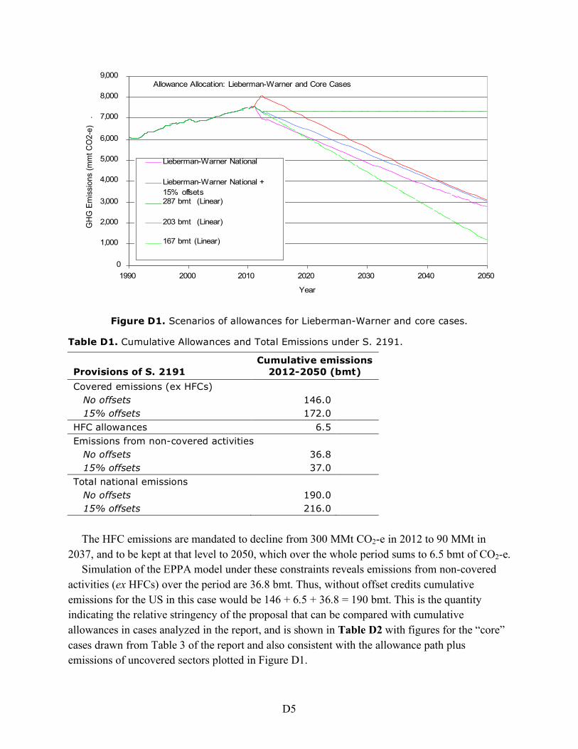
As explained in the report, in a system with banking, such as Lieberman-Warner, and on the assumption that the Act’s target is credible, then the stringency of the system can be represented by the total emissions permitted during the control period (2012 to 2050). We show in Figure D1 a path of allowances plus an estimate of emissions from uncovered sectors for S. 2191 with and without 15% offsets compared with the core cases. We add in emissions from uncovered sectors to the S. 2191 allowance path so that it is possible to see what S. 2191 achieves nationally compared with previous core cases that covered all emissions. We get the estimate of emissions from uncovered sectors from our model simulation of emissions from those sectors when the policy is implemented. The level of emissions from uncovered sectors is just about 1000 mmt CO2-e in 2015, falling to about 900 mmt by the middle of the period and rising to about 950 mmt by 2050. A summary of the available cumulative allowances under the two Lieberman-Warner cases are provided in Table D1. First consider the case with no offsets. For covered emissions other than the HFCs, allowances available under the Act are required to be reduced from 5775 mmt CO2-e in 2012 to 1732 mmt in 2050. Given the specified linear path of decline, this provision sums to 146 bmt CO2-e over the period.

D5

Figure D1. Scenarios of allowances for Lieberman-Warner and core cases.

Table D1. Cumulative Allowances and Total Emissions under S. 2191.

Provisions of S. 2191

Cumulative emissions 2012-2050 (bmt)

Covered emissions (ex HFCs) No offsets 146.0 15% offsets 172.0 HFC allowances 6.5 Emissions from non-covered activities No offsets 36.8 15% offsets 37.0 Total national emissions No offsets 190.0 15% offsets 216.0

The HFC emissions are mandated to decline from 300 MMt CO2-e in 2012 to 90 MMt in

2037, and to be kept at that level to 2050, which over the whole period sums to 6.5 bmt of CO2-e. Simulation of the EPPA model under these constraints reveals emissions from non-covered

activities (ex HFCs) over the period are 36.8 bmt. Thus, without offset credits cumulative emissions for the US in this case would be 146 + 6.5 + 36.8 = 190 bmt. This is the quantity indicating the relative stringency of the proposal that can be compared with cumulative allowances in cases analyzed in the report, and is shown in Table D2 with figures for the “core” cases drawn from Table 3 of the report and also consistent with the allowance path plus emissions of uncovered sectors plotted in Figure D1.

Allowance Allocation: Lieberman-Warner and Core Cases

0

1,000

2,000

3,000

4,000

5,000

6,000

7,000

8,000

9,000

1990 2000 2010 2020 2030 2040 2050

Year

GH

G E

mis

sio

ns (

mm

t C

O2

-e)

.

Lieberman-Warner National

Lieberman-Warner National +

15% offsets287 bmt (Linear)

203 bmt (Linear)

167 bmt (Linear)

D6

Table D2. Cumulative allowances available from 2012 to 2050.

Allowance Path

Cumulative Allowances 2012-2050 (bmt)

Udall-Petri 2006 293 287 bmt 287 Bingaman-Specter 2007 250 (210) Lieberman-Warner 2007, no offsets 190 (153) Lieberman-Warner 2007, 15% offsets 216 (179) 203 bmt 203 Feinstein August 2006 195 Kerry-Snowe 2007 179 Sanders-Boxer 2007 167 167 bmt 167 Waxman 2007 148 Note: For Lieberman-Warner variations and Bingaman-Specter: numbers in parentheses are for

covered sectors only and numbers outside of parenthesis are estimates for total national emissions including uncovered sectors.

Under the assumption of 15% offsets we relax the emissions constraint and it appears from

the accounting in Table D1 that emissions are higher, but assuming that the credit system generates real reductions or an increase in sinks somewhere, the net effect on atmospheric concentrations would be nearly the same as without the credit system. In this case, total allowances for emissions (ex the HFCs) plus offsets is then 146.4/0.85 = 172 bmt. The HFC limit remains the same. The one slight difference that emerges is that when the EPPA model is simulated under this looser set of constraints the economic impacts are reduced leading to a slight increase in estimated emissions from non-covered sectors, from 36.8 to 37.0 bmt. Total national emissions as accounted in Table D1 in this case then sum to 172 + 6.5 + 37 = 216 bmt, however, this accounting excludes changes in domestic land use emissions/sinks and any foreign emissions/sinks brought about by the credit system.3

Note that this approach to including credits should show approximately the correct impact on the CO2-e price if indeed credits are available up to the 15% limit. Welfare impacts are, however, underestimated by this approach unless the credits are domestically supplied at nearly zero real cost. The real cost to the US economy of credits purchased from domestic sources is the inframarginal abatement cost rather than the price actually paid for the credits, since the difference between the price paid and the inframarginal cost simply represent transfers within the US between buyers and sellers of the credits. On the other hand, if all of the credits are purchased from abroad any inframarginal rents are earned by foreign credit sellers and the US welfare cost, at least from a partial equilibrium perspective, is the carbon price times the number credits purchased.

3 If credits were generated from non-covered activities that are accounted in the table, then we would see a

concomitant reduction in emissions of non-covered sectors.

D7

D2.2 Special Treatment of Carbon Capture and Storage

Because of the importance of carbon capture and storage, we also have constructed a scenario that simulates the extra incentives provided for it in the Act. As noted above, the ten-year limit on the incentive for any facility needs to be considered. We have implemented this feature in the EPPA model as follows, in the form of a bonus value for this technology and assuming a CCS plant life of 40 years. Since the EPPA model is recursive dynamic, we calculate the levelized value of the bonus allowances over the lifetime of a CCS plant. The levelized value reflects the fact that a CCS plant is a commitment to a 40 year investment but the bonus allowances are only awarded for 10 years. The levelized value is calculated within the EPPA model and depends on the endogenous CO2-e price and the specified bonus rate. We introduce it as a subsidy to CCS production that changes as a result of competing effects: over time the CO2-e price rises tending to increase the levelized value but the bonus rate is falling and eventually is phased out completely tending to decrease the bonus value eventually to zero. We have not implemented the 4% limit on the bonus award but evaluate whether/when that limit would be exceeded.

To calculate the LevelizedBonusValue, we begin with the discounted BonusValue that would be associated with 1 ton of CO2 storage per year over an assumed 40 year life of a plant, where period 0 is the first period the plant operates:

BonusValue =P

CO2,t! B

t

(1+ r)t

0

39

" (1)

We take advantage of the fact that with banking the CO2-e price rises at the discount rate, r, and thus the 40 year price path can be represented as exponential growth at r of the period 0 price. We then note that the discount term in the denominator cancels the price increase rate term in the numerator:

BonusValue =P

CO2,0(1+ r)t

Bt

(1+ r)t= P

CO2,00

39

! Bt

0

39

! (2)

Finally, the LevelizedBonusValue is the value per ton sequestered in year 0, and so we divide the BonusValue by the 40 tons sequestered over the life of the plant.

LevelizedBonusValue =

PCO2,0

! Bt

0

39

"

40 (3)

This formula conveniently eliminates the need to know CO2-e prices in periods beyond the period of the investment decision, allowing us to calculate the value in the recursive dynamic structure. The intuition of the formula (3) is that even though the actual bonus value is lumped into the first 10 years, the incentive to invest in the plant that bonus value creates must be spread over the full life of the plant given the irreversible nature of the investment.

D8

D3. GREENHOUSE GAS PRICES AND WELFARE COST

As with the analysis in the report for the core cases, the tightening of the target over time results in the banking of allowances, so that the actual pattern of reductions will differ from the paths laid out in Figure D1 (see Figure 2 in the report). First we analyze S. 2191 without the special incentive for CCS investments, and then repeat the simulation with this provision in place to show its potential influence.

D3.1 Case Assuming No CCS Incentive

Prices for the Group of Gases ex HFCs. The results for the CO2-e price and welfare effects are presented in Table D3 and Figure D2. Detailed results are presented in Tables D6 to D9. The initial price is $56/tCO2-e without offset credits (LW) and $48 tCO2-e with credits (LW+15%), and rises to $222 (without offsets) and $190 (with offsets). These results are very close to the original 167 bmt case analyzed in the body of the report which has an initial price of $53 tCO2-e that rises to $210.

Prices for HFCs. The HFCs have quite high GWPs and thus the incentive to reduce them can be very strong for a given CO2-e price. CO2-e prices like those we see in the cases simulated here

Table D3. CO2-equivalent prices (ex HFCs).

CO2-e Price ($/tCO2-e)

LW LW+CSS Subsidy

LW+15% Credits

LW+15% Credits + CCS Subsidy

2015 56 55 48 48 2020 68 67 59 58 2025 83 81 71 71 2030 101 99 87 86 2035 123 120 106 105 2040 150 147 128 128 2045 182 178 156 155 2050 222 217 190 189

Figure D2. Welfare Change.

Welfare Change

-2.00

-1.80

-1.60

-1.40

-1.20

-1.00

-0.80

-0.60

-0.40

-0.20

0.00

2015 2020 2025 2030 2035 2040 2045 2050

Year

Welfa

re C

hange (

%)

.

LW

LW+15% Credits

LW+CCS Subsidy

LW+15%

Credits+CCS Subsidy

D9

typically lead to very high abatement levels of HFC emissions. The separate HFC cap requires reductions in HFC use of only about 50% and so we see very low marginal abatement costs in the separate HFC market, starting at under $.10 per ton CO2-e and rising to about $2.40 per ton. If trade were allowed with the rest of the CO2-e market the prices would equalize and we would see far higher abatement of HFCs, somewhat less abatement in other sectors, and some overall reduction in the cost of the policy. However, HFCs are a relatively small fraction of emissions and so the CO2-e price with trading would likely settle to within a few dollars of the price in the larger market.

Welfare Effects. The welfare effects without credits are almost exactly the same as the 167 bmt case even though the CO2-e prices are slightly higher, but since the cost is across a smaller base, that result should be expected. With the 15% credits the welfare costs are considerably less than the 167 bmt case, and close to the 203 bmt case. The close similarity of the results of S. 2191 to previous runs means that many of the other results and variants produced in the earlier analysis apply to S. 2191—for example, the role of biofuels, emissions trading, the possibility of a second generation of nuclear power, etc. and so those interested in such variants can fairly confidently extrapolate from the previous results.

D3.2 Case with CCS Incentive

We expect the additional incentive for CCS to move up the deployment of CCS and increase the amount of CCS used, especially in early years when the incentive is strong. With more CCS in the electric generation sector the pressure to abate in other sectors will be less and thus we expect the CO2-e price to fall. We do see a slight decrease in CO2-e prices in Table D3 when we add the CCS subsidy to both the LW and LW+15% cases. In the LW case, CO2-e price drops by about $1 per ton CO2-e in 2015 and by about $5 per ton in 2050. In the LW+15% case, the decrease in price is smaller, about $1 or less in all years. However, these results overstate the actual effect of the CCS bonus because, as we will show below, the incentive leads to a potential bonus award that exceeds the 4 percent limit on these allowances as specified in S. 2191.

While we expect the CO2-e price to fall we would in general expect welfare costs to rise because the additional bonus for CCS diverges from equal marginal cost pricing. We see in Figure D2 a slight increase in the welfare cost in early years with the CCS subsidy but then see fairly substantial reductions in the welfare cost in later years compared to comparable cases without the subsidy, suggesting that overall the CCS subsidy leads to a lower net present value welfare cost. This result reflects part of the motivation for such a subsidy whereby the hope would be that by encouraging early demonstration of the CCS technology and creating earlier development of the industries that would support the construction of the plants, one gets lower costs in later years. In an idealized, forward-looking general equilibrium model one would tend not to get this result because agents could look forward to see the gains from earlier demonstration of the technology and thus would deploy it earlier as long as they could fully appropriate the gains from their early investment. Full appropriation of the gains from early investment seems unlikely as firms that waited could still take advantage of lower cost

D10

construction. Thus, there is an argument as to why in reality an extra incentive for CCS could lead to an overall welfare improvement as it would correct the spillover externality that comes with early investment in CCS. This issue is explored in the context of the Netherlands in a study by Otto and Reilly (2006) with a forward looking CGE model with technology externalities explicitly represented. They find welfare benefits from additional subsidy for CCS because of technology spillovers.

The EPPA model does not have as explicit a treatment of the technology spillover decision process. The positive welfare result for the CCS subsidy we see in Figure D2 is the combination of the myopic behavior in the recursive formulation of EPPA and the treatment of constraints on the rate of deployment of new technologies like CCS. In the EPPA model, new technologies are endowed with a limited amount of a technology specific capital referred to as a fixed factor input (Paltsev et al., 2005). This places a limit on how much capacity can be added in early years of deployment. The limit can be overcome by substitution of more labor and capital, but the representation leads to fairly sharply increasing costs as more capacity expansion is attempted. The intuition behind this approach is that the fixed factor endowment represents an initial constrained capacity of trained engineers. Trying to build more plants stretches this limited capacity more thinly and results in extra costs of construction. Expansion of the endowment of the fixed factor in year t+1 is a function of investment in the technology in year t — experience with actually constructing plants leads to more trained engineers in the next period. As a result, the more investment in the new technology in year t that occurs in the model the greater the increase in the fixed factor endowment in the next year.

The parameters of this formulation were estimated to reflect penetration rates seen with nuclear power in the 1960s and 1970s, at that time a new technology that was penetrating rapidly. Because the EPPA structure is recursive dynamic, the decision to invest in period t is made with agents unaware of the benefit in terms of a larger fixed factor it confers in the next (and all future) periods. The way the fixed factor is handled in EPPA thus creates a form of technology spillover because the benefits in the future are not considered in the decision to invest today. This structure explains the results and is an underlying rationale for them, but the way the process is handled in the EPPA model is somewhat ad hoc compared with the more explicit treatment in Otto and Reilly (2006). Modeling the process accurately is computationally intensive and even if that it done completely, the empirical issues involved with estimating possible spillovers for a specific technology are substantial. Thus, the numerical results for welfare effects related to CCS subsidy from these simulations are at best suggestive.

While the welfare results are only suggestive, the fact that a substantial subsidy would encourage earlier development of CCS is expected. Thus we see in Figure D3 and Table D4 the amount of generation in exajoules from coal-based CCS and the amount of CO2 captured and stored when the CCS subsidy is included compared with cases without the subsidy. Whereas CCS does not enter until 2020 without the subsidy we find it enters in 2015 with the subsidy. Not surprisingly, given the structure of the subsidy, it has the biggest effect in the period up to 2035, but there is a lasting effect even beyond 2040 when the subsidy disappears.

D11

Figure D3. CCS Output in EJ.

Table D4. Carbon Sequestered.

Carbon Sequestered (mmt CO2)

LW LW+CSS Subsidy

LW+15% Credits

LW+15% Credits+CCS Subsidy

2015 0 57 0 54 2020 67 173 65 167 2025 156 515 142 449 2030 464 1264 415 1203 2035 1605 2184 1420 1772 2040 2210 2521 2150 2530 2045 2711 2953 2657 2944 2050 3175 3309 3165 3312

In Table D5 we calculate the tons sequestered that would be eligible for bonus allowances

and the fraction of allowances this would require. The legislation allows bonuses to be awarded for the first 10 years of operation, and so we calculate the eligible tons sequestered by accounting the net new sequestration occurring in each year, and assume that allowances can be awarded for two 5-year periods in EPPA. Thus, for example the 57 mmt sequestered in 2015 in the LW+CCS case are eligible for bonus allowances in 2015 and 2020, and we subtract them out of the total tons sequestered in 2025 to calculate the eligible tons in 2025. We then multiply the eligible tons by the bonus rate in each year as specified in S. 2191, and then divide this by the total number of allowances available in each year. The bill limits the amount of bonus allowances for CCS to 4% of the total and we see from this calculation that the potential award exceeds this limit for almost all years, rising to as much as 20 or 25% of the total allowances. Thus, our estimates of the impact of this provision on CCS adoption, coal use, and the CO2-e price are overestimated if this allowance limit is enforced. The program will need to devise some method of rationing the bonus allowances.

CCS Output

0.0

2.0

4.0

6.0

8.0

10.0

12.0

14.0

16.0

18.0

20.0

2015 2020 2025 2030 2035 2040 2045 2050

Year

CC

S O

utp

ut

(EJ)

.

LW

LW+15% Credits

LW+CCS Subsidy

LW+15%

Credits+CCS Subsidy

D12

Table D5. Potential Bonus Allowances for CCS.

Tons of Eligible Emissions

Bonus Rate

Potential Bonuses Awarded

Fraction of Allowances

LW+ CCS

LW+15+CCS

LW+ CCS

LW+15+ CCS

LW+ CCS

LW+15+ CCS

2015 57 54 4.5 257 243 0.05 0.04 2020 173 167 3.6 623 601 0.13 0.12 2025 458 395 2.1 962 830 0.22 0.19 2030 1091 1036 0.9 982 932 0.25 0.24 2035 1669 1323 0.5 835 662 0.25 0.20

Political interest in CCS stems in part from concern about the coal industry. The analysis in

the body of this report tend to show an extended shift to gas generation in the nearer term, with CCS penetration beginning later and only coming on strong after 2030 or so. The result is that the coal industry shrinks and only recovers once CCS technology penetrates the market. The retrenchment of the coal industry would likely cause dislocation in the industry, loss of jobs, and would be a blow to the economic base in states where coal production was important. Thus, one motivation for getting more CCS earlier is to avoid the difficult period in the coal industry. Figure D4 shows for the LW (panel a) and LW+15% (panel b) cases the level of coal production in the US with and without the CCS subsidy. The CCS subsidy clearly does alleviate some of the impacts on the coal industry but it still experiences a period of decline before it recovers. Critical to this result is the specification of the fixed factor, and the ability to substitute for that was discussed above. This formulation does not absolutely limit initial period production of CCS, but it does strongly limit the amount in the first few periods of the model that is determined by the elasticity of substitution between the fixed factor and other inputs and the size of the initial endowment of the fixed factor. It reflects a view that construction of these plants will have to gradually ramp up, and attempts to build many (e.g. dozens of plants) that all come on line at about the same time would be very costly because of the lack of experience. Thus, even with a

Figure D4. Coal Primary Energy Use With and Without the CCS Subsidy: (a) LW, (b) LW+15%

(a) LW Cases With and Without CCS Subsidy

0

5

10

15

20

25

30

35

40

45

2005 2010 2015 2020 2025 2030 2035 2040 2045 2050

Year

Co

al P

rim

ary

En

erg

y U

se

(E

J)

.

LW

LW+CCS

Subsidy

(b) LW+15% With and Without CCS Subsidy

0

5

10

15

20

25

30

35

40

45

2005 2010 2015 2020 2025 2030 2035 2040 2045 2050

Year

Co

al P

rim

ary

En

erg

y U

se

(E

J)

.

LW+15% Offsets

LW+15%

Offsets+CCS Subsidy

D13

very strong subsidy, the number of plants must gradually ramp up. That representation of the process combined with the fairly strong reductions needed to meet the caps in this legislation lead inevitably to a cut back in coal production. Increasing the bonus allowance rate would not significantly speed up the introduction of these plants at least as the EPPA model is formulated because the critical elasticity is relatively low. One might question the specific formulation of this process in EPPA, but the idea that it takes some time to ramp up an industry is fairly widespread. At issue is the degree to which additional economic incentives can speed up the process.

D4. FEATURES OF THE ACT NOT COVERED IN THE ANALYSIS

We are able to represent some of the main features of the cap and trade measures laid out in S. 2191, but there are many important features of the bill that are difficult to quantify in a model like EPPA or that were simply beyond the scope of the analysis we conducted. We briefly identify some of the more important features here.

D4.1 A Changing Mix of Free Allocation and Auctioning

The Act specifies the free distribution of allowances in some detail. In addition, a significant proportion of allowances—22.5% in 2012 rising to 70.5% by 2031—are slated to be auctioned by a Climate Change Credit Corporation (CCCC). Auction revenue is to be used for a host of purposes from mitigating impacts on low-income energy consumers and promoting energy efficiency and technology development to addressing impacts of climate change. To the extent R&D is successful that could reduce the direct costs of the climate cap-and-trade components of the legislation. Similarly, promotion of energy efficiency provides incentives beyond the CO2-e price embedded in energy prices to conserve energy and would tend to reduce the direct costs of cap and trade components of the legislation. It is very difficult to assess how much technology development or additional efficiency one can achieve with such programs. And the gains in terms of lower direct costs associated with the cap-and-trade program need to balanced against the opportunity cost of the money used to support these programs that otherwise could be returned back to citizens in a lump-sum manner or used, as some have proposed, to reduce other distortionary taxes.

D4.2 Interaction with Other Incentives

The economic logic of cap-and-trade systems leads to a recommendation of lump-sum distribution or auction of allowances so that an equal signal is sent to all covered activities regarding the marginal value of abatement. Creating additional incentives for emissions reduction, either with the revenue or the allowance distribution, can create distortions that erode the economic efficiency benefits of an idealized cap-and-trade implementation. Missing in such a textbook system, of course, is the fact that some activities may be outside the cap. The usual approach for including them is through a crediting system, which the bill includes as discussed above.

D14

S. 2191 introduces an innovation in that it also uses allowance distribution and revenue allocation, in part, to extend incentives for the-cap-and trade program beyond the capped entities. For example, 5% of allowances are dedicated for use in agriculture and forestry to encourage sinks related to land use. This provision is separate from the one that allows these sectors to produce credits to be sold into the allowance market (and it specifically prohibits land sinks from benefiting from both the sale of credit and the awarding of an allowance). The combined effect of these provisions is to extend the incentives of a credit system beyond the 15% limit. But because the allowance incentive removes the allowances from the general pool, it is not an open-ended credit system, and this distribution should not affect the CO2-e price within the capped system. Any allowances distributed in this way simply reduce the number either given to capped entities or auctioned, but then those receiving them would sell them back to capped entities and so there is no net change in the total allowances available. In contrast, a credit system tends to reduce the CO2-e price in the system by creating credits that can be used in place of allowances. Other activities covered under this provision include methane from land fills and coal mining and international forest protection. On top of this, some of the auction revenue is also directed to be used to create such incentives.

The provisions of the legislation thus create as many as three different mechanisms directed toward creating incentives for non-capped sectors. The overall structure ties the level of incentive per ton abated to the market price for CO2 and the legislation’s instructions are to avoid overlap—that is entities could not sell credits into the system and also have allowances awarded to them for the same ton of CO2. Thus, this approach has some desirable efficiency attributes by relating the value of abatement in these programs to the CO2-e price. However, both awarding allowances outside of the capped system and funding programs with auction revenue face the same difficulties of a traditional credit system—requiring the development of a counterfactual baseline for qualifying projects and activities to determine the level of real additional abatement. The bureaucratic process that results tends to limit the amount of abatement that can qualify, and the project-by-project approach may create a situation where significant leakage occurs—an enhanced forest sink receiving allowances or payments may be offset by a reduction in a sink somewhere else, given an unchanged overall demand for land conversion.

D4.3 The Cost Control Mechanism

A Federal Carbon Market Efficiency Board is established whose function is to monitor the allowance trading system. Apart from reporting to Congress, the primary power of the Board is to increase opportunities to borrow allowances from future allocations—i.e., to increase the allocation available in the near-term while imposing a compensating reduction in the future. The Board may do this by relaxing the limits on borrowing by regulated entities (private borrowing), or it may itself temporarily issue more allowances, providing it then reduces those available in the future (a form of public borrowing).

Because the prescribed allowance path imposes ever greater stringency with time the system is strongly biased at the outset toward net banking rather than net borrowing. Private firms would

D15

tend to bank allowances in early periods and, if that is the case, efforts by an Efficiency Board to borrow from the future could be frustrated by the action of private agents to bank the additional allowances in anticipation of the tightening future constraint. There may be some value to this feature if for some reason early in the program unusual conditions lead to exceptionally high demand for allowances and a spike in their price. However, such conditions could easily be interpreted by private agents as evidence that the stringency of the program had been underestimated, and that the whole future price path should be expected to stay higher than anticipated. Private entities would then simply bank the allowances brought forward, frustrating the Board’s efforts to control costs in the short run. While intended to provide the Board with ability to limit costs, this provision probably provides it little real power to do so.

D4.4 Potential Coverage of Large Land Operations

It appears that the intent of the bill is to include land use emissions and sinks only through relatively high transaction-cost provisions for offset credits (and allowance and revenue allocation) described above. However, it seems possible that larger land holders could be included as a “Covered Facility” as defined in Section 4, Paragraph 7 should the EPA Administrator choose to include them, and thus could be brought fully under the cap-and-trade program. In particular, a covered facility can include:

“. . . any facility that in any year produces, or any entity that in any year imports, more than 10,000 carbon dioxide equivalents of chemicals that are class I greenhouse gases, assuming no capture and destruction of or permanent storage.”

As we read this text (without access to the intent of the authors) is appears that a large forest company that in harvesting a forest produced 10,000 tons of CO2 emissions could be a covered facility. The initial definition of a “facility” is “1 or more buildings, structures, or installations on 1 or more contiguous or adjacent property.” However, the Act states that:

“at the option of the Administrator, a facility can include any activity or operation that emits 10,000 carbon dioxide equivalents in any year; and has a technical connection with activities carried out at a facility, such as the use of transportation fleets, pipelines, transmissions lines, and distribution lines, but that is not conducted or located on the property of the facility.”

Thus, for example, a large forest company has mills (structures) that are technically connected to forest land through a transportation system (that brings logs to the mill), and emissions related to logging—even if they do not occur at the mill itself—could be counted together to add up to 10,000 tons of CO2. Moreover, emissions only need exceed the 10,000 ton limit in “any” year, and so if when the land is harvested the limit was exceeded the facility (i.e. the mill and the land) would remain covered even as regrowth occurred and the land acted as a CO2 sink.

If this interpretation of the bill were exercised we believe this would be a positive development in bringing all large US land holders fully within a cap-and-trade system. Other analysts with whom we have discussed this provision believe this is not the intention of the legislation. Supporting their interpretation are summaries of the bill that are more explicit in

D16

suggesting covered facilities are those that produce for sale or distribution 10,000 tons of CO2 equivalent. They argue that land use CO2 emissions are a by-product, not produced for sale or distribution, and that this component of the definition of covered facility is intended to cover SF6 and PFCs—manufactured gases produced for sale and distribution. However, the language in the bill itself does not include “sale and distribution” terms which appear only in a simplified summary. As we argued elsewhere (Reilly and Asadoorian, 2007), there is nothing in principle that prevents land use emissions from being included within a cap-and-trade system, and the fact that the language in S. 2191 could be easily be interpreted to include them seems to make that point. Incorporation of major land users within the cap-and-trade program could have substantial effects on the overall costs of the program depending on how baselines were established for covered entities. Given that US forests are currently a net sink, if baselines were set at zero the inclusion of forests would significantly reduce costs because the existing net sink would essentially relax the constraint. Assuming that baseline issue were addressed in a way that assured additionality, one would still expect considerable cost savings by effectively bringing within the cap-and-trade system another set of activities with additional low-cost abatement options.

D5. CONCLUSIONS

The analysis in this appendix supplements the main report by providing an evaluation of the cap-and-trade components of S. 2191 developed as a compromise bill after the completion of the body of this report. The analysis presented here represents the main quantitative features of the proposed cap-and-trade system. The results suggest that overall carbon price and economic welfare effects are similar to cases analyzed in the body of the report. We have therefore not extensively investigated alternative scenarios and sensitivities to key assumptions in this appendix. The general results from the sensitivity studies in the body of the report remain valid for the new legislation. The novel features of the legislation included in our quantitative analysis is the move upstream in the coverage of energy, separation of the HFC allowance market from the allowance market for other abatement, and bonus allowances awarded to carbon capture and storage (CCS). The upstream nature of the system means that nearly all fossil energy emissions are included under the cap, with emissions of non-CO2 GHGs from agricultural and waste activities being the biggest category of domestic emissions that remain outside the system. The separate HFC market is, according to our analysis, far less tightly constrained than the primary market, leading to much lower CO2-e prices than in the main CO2 market. The bonus allowance awards for CCS provide a substantial incentive to speed up deployment of CCS, but they do not completely eliminate the retrenchment of the coal industry in the first decade or so of the cap-and-trade program. As in some previous legislation, there are provisions for credits from outside the system limited to 15% of total emissions, with potentially an additional 15% of emissions accounted for by allowances from foreign trading systems such as the ETS. We find that availability of credits would reduce CO2-e prices from the case without credits by about $8/tCO2-e in 2015, rising to a savings of almost $32/tCO2-e by 2050. We did not analyze cases

D17

that simulate credits from foreign trading systems as that effect could be either to reduce or to increase the allowance price depending on the stringency of the foreign system with which the US system was linked.

There are other features of the bill that we did not analyze that will be important in implementation of the legislation if some form of it were to enter into law. Some of these features include the use of auction revenue, how allowances are awarded to encourage abatement beyond the covered sectors, the role of the Federal Carbon Market Efficiency Board, and the latitude given to the EPA Administrator to extend the definition of covered entities. Directing revenue toward R&D and to efficiency would likely reduce the direct costs of the cap-and-trade system, but at the opportunity cost of these funds if they were alternatively either distributed back to consumers or used in other ways. The use of allowances and auction revenue as incentives for additional abatement outside of the capped sectors represents an interesting way to extend the boundaries of the program to influence emissions beyond the capped sectors, but it would not affect costs within the trading system in our evaluation. Expansive interpretation of the latitude given to the EPA Administrator to define a facility could, in our interpretation, be read to include entities with large land use emissions or potential sinks. This extension could substantially reduce costs of the program, but analysis of that potential was beyond the scope of this brief analysis.

D6. REFERENCES

Otto, M.V., and J. Reilly, 2006: Directed Technical Change and the Adoption of CO2 Abatement Technology: The Case of CO2 Capture and Storage. MIT Joint Program Report 139, Cambridge, MA (August); http://mit.edu/globalchange/www/MITJPSPGC_Rpt139.pdf.

Paltsev, S., J.M. Reilly, H.D. Jacoby, R.S. Eckaus, J. McFarland, M. Sarofim, M. Asadoorian and M. Babiker, 2005: The MIT Emissions Prediction and Policy Analysis (EPPA) Model: Version 4. MIT Joint Program Report 125, Cambridge, MA (August); http://mit.edu/globalchange/www/MITJPSPGC_Rpt125.pdf.

Reilly, J., and M. Asadoorian, 2007: Mitigation of Greenhouse Gas Emissions from Land Use: Creating Incentives within Greenhouse Gas Emissions Trading Systems. Climatic Change, 80:173-197; available as MIT Joint Program Reprint 2007-1 (http://mit.edu/globalchange/www/MITJPSPGC_Reprint07-1.pdf).

D18

Table D6. Lieberman-Warner (No Offsetts, No CCS Subsidy)

2005 2010 2015 2020 2025 2030 2035 2040 2045 2050

ECONOMY WIDE INDICATORS

Population (million) 296 309 321 334 347 359 369 379 388 397 GDP (billion 2005$) 11981 14339 16810 19637 22760 26377 30236 34679 39148 43724

% Change GDP from Reference 0.00 0.00 -0.65 -0.69 -0.38 -0.31 -0.97 -0.72 -0.97 -1.10

Market Consumption (billion 2005$) 8217 9858 11492 13262 15154 17418 20053 22833 25812 28870

% Change Consumption from Reference 0.00 0.00 -0.35 -0.92 -1.36 -1.93 -2.02 -2.39 -2.43 -2.36

Welfare (billion 2005$) 9656 11773 13923 16250 18759 21692 25035 28494 32166 35893

% Change Welfare from Reference(EV) 0.00 0.00 -0.07 -0.56 -0.99 -1.47 -1.49 -1.85 -1.87 -1.81

CO2-E Price (2005$/tCO2-e) 0.00 0.00 56.14 68.30 83.10 101.11 123.01 149.66 182.09 221.54

PRICES (index, 2005=1.00)

Petroleum Product 1.00 1.15 1.28 1.39 1.38 1.40 1.22 1.19 1.21 1.21 Natural Gas 1.00 1.11 1.14 1.38 1.70 1.97 1.97 1.99 1.96 1.87

Coal 1.00 1.04 1.00 0.98 0.97 0.97 1.02 1.07 1.11 1.15

Electricity 1.00 1.11 1.61 1.74 1.66 1.81 1.74 1.62 1.61 1.61

TRADE & PRODUCTION (selected indicators)

Bio Liquids Production in US (EJ) 0.0 0.0 0.0 0.0 0.0 0.0 0.0 0.0 3.9 5.6

Net Bio Liquids Imports (EJ) 0.0 0.0 0.3 7.3 17.6 28.7 18.1 31.0 29.8 29.6

Net Bio Liquids Imports (billion 2005$) 0.00 0.00 1.83 39.14 94.19 153.36 96.92 165.48 159.17 158.17

Net Crude Oil Imports (billion 2005$) 77.40 85.21 70.97 52.61 32.15 5.92 71.27 40.20 42.51 50.82

Net Agriculture Exports (billion 2005$) 25.64 25.53 12.23 12.33 9.91 10.21 11.82 15.41 1.78 -2.27

GHG EMISSIONS (mmt CO2-e)

GHG Emissions 7091.9 7680.1 6725.7 5903.7 5158.6 4195.1 4374.8 3656.2 3583.2 3605.9

CO2 Emissions 5984.3 6517.4 5525.6 4766.5 4069.7 3164.1 3400.9 2667.7 2575.2 2570.4

CH4 Emissions 583.4 602.0 564.7 541.5 527.8 527.0 523.0 544.6 558.7 571.0

N2O Emissions 385.2 387.9 360.0 348.5 343.1 341.5 345.5 354.5 359.8 375.2

Fluorinated Gases Emissions 140.0 173.8 276.4 248.3 219.0 163.4 106.3 90.3 90.3 90.3

PRIMARY ENERGY USE (EJ)

Coal 22.6 24.3 18.0 12.6 10.4 10.6 18.1 26.1 32.4 38.2 Petroleum Products 42.0 46.0 41.1 35.4 27.3 18.5 33.0 23.0 23.1 24.6

Including Shale Oil 0.0 0.0 0.0 0.0 0.0 0.0 0.0 0.0 0.0 0.0

Natural Gas 22.5 24.7 23.5 27.8 31.3 30.8 26.4 23.1 19.7 16.7

Nuclear (primary energy eq) 9.3 9.0 8.9 8.9 8.5 8.3 8.2 8.2 8.2 8.2

Hydro (primary energy eq) 2.9 2.8 3.2 3.2 3.1 3.1 3.1 3.1 3.2 3.3

Renewable Elec. (primary energy eq) 0.6 0.7 0.9 1.1 0.9 1.2 1.1 1.4 1.5 1.6

Biomass Liquids 0.0 0.0 0.3 7.3 17.6 28.7 18.1 31.0 33.7 35.2

Total Primary Energy Use 99.8 107.6 95.9 96.4 99.1 101.3 108.1 115.8 121.8 127.7

Reduced Use from Reference 0.0 0.0 18.6 24.1 27.7 33.3 35.8 37.3 40.1 42.2

ELECTRICITY PRODUCTION (EJ)

Coal w/o CCS 6.9 7.6 6.0 3.9 3.0 2.2 0.0 0.0 0.0 0.0

Oil w/o CCS 0.3 0.3 0.2 0.2 0.1 0.1 0.0 0.0 0.0 0.0

Gas w/o CCS 2.1 2.5 3.1 5.3 7.2 6.4 3.9 2.8 1.5 0.4

Nuclear 3.0 3.0 3.1 3.2 3.1 3.1 3.1 3.1 3.1 3.1

Hydro 0.9 1.0 1.1 1.1 1.1 1.2 1.2 1.2 1.2 1.3

Other Renewables 0.2 0.2 0.1 0.7 0.3 0.5 0.4 0.5 0.6 0.6

Gas with CCS 0.0 0.0 0.0 0.3 0.6 1.6 2.2 1.4 1.1 0.7

Coal with CCS 0.0 0.0 0.0 0.3 0.6 1.8 7.7 11.5 14.6 17.3

Total Electricity Production 13.4 14.6 13.7 14.9 16.0 16.9 18.5 20.6 22.0 23.4

D19

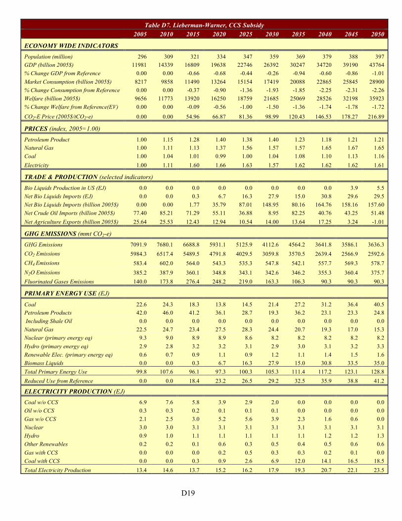
Table D7. Lieberman-Warner, CCS Subsidy

2005 2010 2015 2020 2025 2030 2035 2040 2045 2050






Welfare (billion 2005$) 9656 11773 13920 16250 18759 21685 25069 28526 32198 35923


CO2-E Price (2005$/tCO2-e) 0.00 0.00 54.96 66.87 81.36 98.99 120.43 146.53 178.27 216.89



Coal 1.00 1.04 1.01 0.99 1.00 1.04 1.08 1.10 1.13 1.16

Electricity 1.00 1.11 1.60 1.66 1.63 1.57 1.62 1.62 1.62 1.61






Net Agriculture Exports (billion 2005$) 25.64 25.53 12.43 12.94 10.54 14.00 13.64 17.25 3.24 -1.01


GHG Emissions 7091.9 7680.1 6688.8 5931.1 5125.9 4112.6 4564.2 3641.8 3586.1 3636.3

CO2 Emissions 5984.3 6517.4 5489.5 4791.8 4029.5 3059.8 3570.5 2639.4 2566.9 2592.6

CH4 Emissions 583.4 602.0 564.0 543.3 535.3 547.8 542.1 557.7 569.3 578.7

N2O Emissions 385.2 387.9 360.1 348.8 343.1 342.6 346.2 355.3 360.4 375.7





Natural Gas 22.5 24.7 23.4 27.5 28.3 24.4 20.7 19.3 17.0 15.3




Biomass Liquids 0.0 0.0 0.3 6.7 16.3 27.9 15.0 30.8 33.5 35.0




Coal w/o CCS 6.9 7.6 5.8 3.9 2.9 2.0 0.0 0.0 0.0 0.0

Oil w/o CCS 0.3 0.3 0.2 0.1 0.1 0.1 0.0 0.0 0.0 0.0

Gas w/o CCS 2.1 2.5 3.0 5.2 5.6 3.9 2.3 1.6 0.6 0.0

Nuclear 3.0 3.0 3.1 3.1 3.1 3.1 3.1 3.1 3.1 3.1

Hydro 0.9 1.0 1.1 1.1 1.1 1.1 1.1 1.2 1.2 1.3


Gas with CCS 0.0 0.0 0.0 0.2 0.5 0.3 0.3 0.2 0.1 0.0

Coal with CCS 0.0 0.0 0.3 0.9 2.6 6.9 12.0 14.1 16.5 18.5


D20

Table D8. Lieberman-Warner, 15%Offsets

2005 2010 2015 2020 2025 2030 2035 2040 2045 2050






Welfare (billion 2005$) 9656 11773 13926 16279 18809 21757 25212 28684 32257 35964


CO2-E Price (2005$/tCO2-e) 0.00 0.00 48.14 58.57 71.26 86.70 105.49 128.34 156.15 189.98



Coal 1.00 1.04 1.01 0.99 0.97 0.96 1.02 1.08 1.11 1.15

Electricity 1.00 1.11 1.56 1.70 1.64 1.79 1.75 1.61 1.61 1.60






Net Agriculture Exports (billion 2005$) 25.64 25.53 13.28 11.33 8.07 7.82 6.35 11.75 4.72 0.27


GHG Emissions 7091.9 7680.1 6863.2 6362.9 5802.7 4838.9 5974.9 4845.3 3855.1 3768.4

CO2 Emissions 5984.3 6517.4 5655.7 5219.3 4717.1 3816.8 4993.2 3851.7 2838.4 2723.6

CH4 Emissions 583.4 602.0 569.8 546.7 524.7 518.7 530.3 548.8 564.9 578.1

N2O Emissions 385.2 387.9 362.4 349.6 343.1 340.8 345.4 354.8 361.8 376.7





Natural Gas 22.5 24.7 24.0 28.3 32.7 33.7 27.7 25.0 21.8 18.6




Biomass Liquids 0.0 0.0 0.4 2.8 9.2 19.5 0.0 16.6 32.3 35.2




Coal w/o CCS 6.9 7.6 6.2 4.1 2.6 1.4 0.4 0.0 0.0 0.0

Oil w/o CCS 0.3 0.3 0.2 0.2 0.1 0.1 0.0 0.0 0.0 0.0

Gas w/o CCS 2.1 2.5 3.2 5.4 8.0 7.8 5.2 3.7 2.2 0.7

Nuclear 3.0 3.0 3.1 3.1 3.1 3.1 3.1 3.1 3.1 3.1

Hydro 0.9 1.0 1.1 1.1 1.1 1.2 1.2 1.2 1.2 1.3


Gas with CCS 0.0 0.0 0.0 0.3 0.5 1.2 0.8 0.6 0.4 0.3

Coal with CCS 0.0 0.0 0.0 0.3 0.6 1.8 7.4 11.7 14.7 17.6


D21

Table D9. Lieberman-Warner, 15% Offsets and CCS Subsidy

2005 2010 2015 2020 2025 2030 2035 2040 2045 2050






Welfare (billion 2005$) 9656 11773 13923 16274 18816 21773 25251 28720 32283 35990


CO2-E Price (2005$/tCO2-e) 0.00 0.00 47.87 58.24 70.86 86.21 104.89 127.61 155.26 188.90



Coal 1.00 1.04 1.01 1.00 1.00 1.04 1.07 1.10 1.14 1.16

Electricity 1.00 1.11 1.55 1.65 1.60 1.57 1.61 1.62 1.61 1.61






Net Agriculture Exports (billion 2005$) 25.64 25.53 13.36 11.81 8.92 11.46 9.16 12.89 6.35 1.25


GHG Emissions 7091.9 7680.1 6813.2 6324.6 5820.9 4888.7 6162.1 4840.8 3806.5 3760.2

CO2 Emissions 5984.3 6517.4 5607.2 5180.9 4720.2 3831.8 5151.6 3834.0 2779.0 2708.5

CH4 Emissions 583.4 602.0 568.6 546.8 538.8 551.6 556.6 562.2 575.8 585.3

N2O Emissions 385.2 387.9 362.2 349.6 343.8 342.9 347.8 355.3 362.4 377.2





Natural Gas 22.5 24.7 23.8 27.9 29.1 25.1 23.0 19.9 17.7 16.0




Biomass Liquids 0.0 0.0 0.3 2.6 8.8 18.9 0.1 15.5 32.2 35.1




Coal w/o CCS 6.9 7.6 6.0 3.9 3.0 2.1 1.4 0.0 0.0 0.0

Oil w/o CCS 0.3 0.3 0.2 0.2 0.1 0.1 0.1 0.0 0.0 0.0

Gas w/o CCS 2.1 2.5 3.1 5.2 6.2 4.3 3.3 1.8 0.8 0.0

Nuclear 3.0 3.0 3.1 3.1 3.1 3.1 3.1 3.1 3.1 3.1

Hydro 0.9 1.0 1.1 1.1 1.1 1.1 1.1 1.2 1.2 1.3


Gas with CCS 0.0 0.0 0.0 0.2 0.1 0.1 0.1 0.1 0.0 0.0

Coal with CCS 0.0 0.0 0.3 0.8 2.5 6.7 9.9 14.2 16.6 18.6


appendix d: analysis of the cap and trade features of the...

Documents