appendix: methods and tables - anu...
TRANSCRIPT

335
Appendix: Methods and tables
Statistical significance, confidence intervals and sourcesIn all Tables, ** indicates statistical significance at 0.01 or better (99 out of 100 possible samples) and * indicates significance at 0.05 (19 out of a possible 20 samples).
In most figures, confidence intervals at the 95 per cent level have been added. In post-estimation, sometimes statistically significant findings do have confidence intervals that overlap. We report this where necessary, leaving it up to readers to decide for themselves how reliable and robust they consider our findings to be.
All data is drawn from New Zealand Election Study (NZES) 2014, unless noted otherwise.
WeightingOur dataset contains oversamples of young people and the Māori electorates and is affected by non-response bias that is based on political interest, political knowledge, education and turnout behaviour. We have weighted to correct for oversampling by gender, age and Māori electorates on a cell by cell basis, and on top of that by education, reported vote and validated turnout, on the basis of iterative weighting on the marginal frequencies. For users of the dataset, the weight variable is dwtfin.

A BARk BuT No BITE
336
Cha
pter
4Ta
ble
4.A1
: Mul
tinom
ial l
ogis
tic re
gres
sion
par
ty c
hoic
e at
the
2014
ele
ctio
n (re
fere
nce
cate
gory
=Nat
iona
l; N
=258
1)N
ot v
otin
gLa
bour
Gre
enN
Z Fi
rst
Con
serv
ativ
eO
ther
Coe
ffr.s
.e.†
Coe
ffr.s
.e.
Coe
ffr.s
.e.
Fem
ale (m
ale)
0.00
60.
200
0.21
20.
147
0.27
70.
196
–0.4
01*
0.20
3–0
.565
0.33
6–0
.278
0.36
6Ag
e (1
8 >)
–0.0
15*
0.00
60.
000
0.00
5–0
.038
**0.
006
0.00
40.
007
–0.0
090.
011
–0.0
030.
011
(Eur
opea
n an
d ot
her)
Māo
ri1 .
768
**0.
311
1.48
3**
0.26
80.
871
**0.
321
1.60
7**
0.36
5–1
.202
1.07
33 .
663
**0.
344
Pasifi
ka1 .
686
*0.
653
1.58
4*
0.64
3–0
.366
0.86
91 .
317
0.83
6–1
5.16
9**
0.62
52.
360
*1.
093
Asian
0.72
90.
382
–0.0
900.
309
–1.8
38**
0.52
3–1
6.32
3**
0.24
3–0
.817
0.72
81.
410
0.78
1(M
id-e
duca
tion)
Low
edu
catio
n–0
.225
0.22
7–0
.057
0.17
7–0
.309
0.24
6–0
.120
0.23
80.
403
0.38
4–0
.217
0.35
9hi
gh e
duca
tion
–0.5
520.
296
0.56
6**
0.20
20.
869
**0.
219
0.00
20.
297
0.29
50.
391
0.24
80.
491
Relat
ive in
com
e (1
–5)
–0.1
410.
101
–0.5
08**
0.08
5–0
.379
**0.
102
–0.5
51**
0.12
2–0
.500
**0.
167
–0.6
17**
0.23
6(P
rivat
e)Pu
blic
sect
or0.
241
0.27
00.
339
0.18
90.
134
0.21
60.
165
0.25
20.
492
0.38
90.
123
0.34
5Se
lf-em
ploy
ed0.
175
0.28
1–0
.184
0.22
60.
487
0.27
3–0
.484
0.27
50.
083
0.34
50.
025
0.48
0(N
on-m
anua
l)M
anua
l0.
231
0.24
00.
631
**0.
177
0.00
00.
257
0.14
50.
250
–0.2
890.
385
–0.5
820.
408
Farm
ing
hous
ehol
d0.
151
0.46
8–0
.644
0.54
4–1
.338
*0.
585
–0.9
240.
590
–0.6
000.
537
–0.1
080.
753
No o
ccup
atio
n Re
porte
d0.
442
0.48
4–0
.594
0.43
30.
000
0.69
30.
643
0.58
0–1
.838
1.10
8–1
.481
0.88
7
unio
n ho
useh
old
0.30
00.
291
0.92
2**
0.20
50.
721
**0.
231
0.56
20.
295
0.24
70.
458
0.02
80.
383

337
APPENdIxN
ot v
otin
gLa
bour
Gre
enN
Z Fi
rst
Con
serv
ativ
eO
ther
Coe
ffr.s
.e.†
Coe
ffr.s
.e.
Coe
ffr.s
.e.
Chur
ch a
ttend
ance
(0
–1)
–0.0
360.
332
0.18
40.
217
–0.8
10*
0.38
60.
373
0.29
72.
010
**0.
333
–0.4
040.
403
Asse
ts s
cale
(0–4
)–0
.334
**0.
093
–0.3
89**
0.07
3–0
.247
**0.
084
–0.0
970.
104
0.13
90.
183
–0.1
250.
154
on
bene
fit (n
ot)
0.26
70.
248
0.26
50.
190
0.30
30.
235
–0.2
710.
310
–0.3
980.
486
0.33
30.
387
Majo
r urb
an (n
ot)
0.01
00.
204
0.10
60.
151
0.39
1*
0.18
4–0
.331
0.21
2–0
.229
0.30
4–0
.080
0.32
1Co
nsta
nt1.
285
*0.
568
0.92
9*
0.45
61.
431
**0.
539
0.19
60.
613
–1.2
380.
790
–0.4
921 .
361
R-sq
uare
d 0.
113
Note
: The
bas
eline
mod
el em
ploy
s m
ultin
omial
logi
stic
regr
essio
n, w
ith p
arty
vot
e fo
r the
Nat
iona
l Par
ty a
s th
e ba
selin
e ca
tego
ry. T
his
is on
e of
the
best
fo
rms
of m
ultiv
ariat
e an
alysis
for a
n un
orde
red
set o
f cat
egor
ies. B
y in
cludi
ng n
ot v
otin
g an
d all
oth
er p
artie
s in
the
mod
el, a
ll cho
ices
are
acco
unte
d fo
r and
se
t aga
inst
eac
h ot
her.
The
othe
r cat
egor
y in
clude
s th
e M
āori
Party
, Int
erne
t-MAN
A, th
e AC
T Pa
rty, u
nite
d Fu
ture
and
all o
ther
par
ties.
Bec
ause
thes
e ar
e a
mixt
ure
of q
uite
diffe
rent
par
ties,
the
cate
gory
is in
the
mod
el to
be
adde
d in
to th
e ov
erall
pat
tern
but
are
of li
ttle
relev
ance
in th
emse
lves.
Not
votin
g is
also
inclu
ded,
but
will
be d
iscus
sed
in c
hapt
er 1
1. T
he fig
ures
in th
is ch
apte
r and
thos
e fo
llow
ing
are
usua
lly p
ost-e
stim
atio
n pr
obab
ilities
der
ived
from
the
mod
el,
usin
g th
e po
st-e
stim
atio
n co
mm
and
mar
gins
in S
tata
, the
sta
tistic
al an
alysis
sof
twar
e pr
imar
ily u
sed
for t
his
book
. Si
gnific
ance
: * p
< 0.
05; *
* p<
0.01
.† r
.s.e
. = ro
bust
sta
ndar
d er
ror.
Tabl
e 4.
A2: M
ultin
omia
l log
istic
regr
essi
on p
arty
cho
ice
at th
e 20
14 e
lect
ion,
with
par
enta
l par
ty id
entifi
catio
n an
d in
com
e/as
sets
inte
ract
ion
(refe
renc
e ca
tego
ry=N
atio
nal;
N=2
581)
Not
vot
ing
Labo
urG
reen
NZ
Firs
tC
onse
rvat
ive
Oth
erC
oeff
r.s.e
.C
oeff
r.s.e
.C
oeff
r.s.e
.Fe
male
(male
)0.
005
0.20
10.
228
0.15
50.
266
0.19
5–0
.392
0.20
6–0
.564
0.34
5–0
.303
0.36
8Ag
e (1
8 >)
–0.0
15*
0.00
6–0
.003
0.00
5–0
.042
**0.
007
–0.0
010.
007
–0.0
070.
010
–0.0
040.
010
(Eur
opea
n an
d ot
her)
Māo
ri1.
574
**0.
316
1.17
0**
0.28
20.
565
0.33
61.
224
**0.
368
–1.1
441.
072
3.40
6**
0.34
0

A BARk BuT No BITE
338
Not
vot
ing
Labo
urG
reen
NZ
Firs
tC
onse
rvat
ive
Oth
erC
oeff
r.s.e
.C
oeff
r.s.e
.C
oeff
r.s.e
.Pa
sifika
0.64
80.
401
0.05
30.
329
–1.6
40**
0.52
0–1
4.51
4**
0.26
7–0
.777
0.73
11.
245
0.76
9As
ian1.
339
*0.
663
1.35
4*
0.62
3–0
.672
0.88
20.
873
0.83
2–1
3.39
5**
0.65
21.
409
1 .16
3(M
id-e
duca
tion)
Low
edu
catio
n–0
.287
0.22
6–0
.204
0.18
8–0
.428
0.24
7–0
.239
0.24
20.
370
0.38
1–0
.249
0.36
5hi
gh e
duca
tion
–0.5
270.
295
0.59
7**
0.21
30.
861
**0.
226
0.07
10.
306
0.28
10.
387
0.33
70.
484
Relat
ive in
com
e (1
–5)
–0.3
780.
219
–0.7
02**
0.19
0–0
.279
0.19
6–0
.217
0.28
3–0
.178
0.55
0–0
.828
*0.
323
(Priv
ate)
Publ
ic se
ctor
0.20
40.
272
0.18
00.
200
0.00
90.
223
0.00
20.
259
0.47
50.
390
0.04
40.
351
Self-
empl
oyed
0.08
60.
288
–0.2
510.
233
0.42
80.
264
–0.5
400.
283
0.08
90.
356
–0.0
820.
493
(Non
-man
ual)
Man
ual
0.24
20.
239
0.57
5**
0.18
7–0
.079
0.25
30.
071
0.25
2–0
.279
0.38
6–0
.588
0.41
1Fa
rmin
g ho
useh
old
0.43
90.
469
–0.1
450.
517
–1.0
540.
606
–0.4
090.
589
–0.5
520.
555
0.30
60.
728
No o
ccup
atio
n Re
porte
d0.
496
0.45
3–0
.502
0.43
50.
185
0.67
50.
809
0.57
6–1
.798
1.11
2–1
.366
0.87
2
unio
n ho
useh
old
0.31
70.
302
0.98
0**
0.22
00.
751
**0.
233
0.59
5*
0.29
60.
223
0.45
80.
025
0.39
2Ch
urch
atte
ndan
ce
(0–1
)0.
057
0.32
40.
311
0.23
4–0
.681
0.38
50.
481
0.31
11.
972
**0.
328
–0.2
800.
399
Asse
ts s
cale
(0–4
)–0
.588
*0.
243
–0.6
05**
0.21
3–0
.091
0.22
10.
268
0.26
00.
454
0.39
3–0
.298
0.48
6o
n be
nefit
(not
)0.
253
0.25
10.
317
0.20
20.
394
0.23
5–0
.145
0.31
1–0
.342
0.49
20.
355
0.36
9M
ajor u
rban
(not
)–0
.024
0.20
20.
016
0.15
70.
315
0.18
5–0
.394
0.21
5–0
.227
0.30
7–0
.129
0.29
5Pa
rent
s La
bour
(0–2
)0.
045
0.12
50.
567
**0.
097
0.65
7**
0.12
00.
660
**0.
133
–0.0
670.
213
0.12
50.
168
Pare
nts
Natio
nal
(0–2
)–0
.532
**0.
148
–0.7
44**
0.13
9–0
.223
0.12
3–0
.398
*0.
168
–0.1
230.
173
–0.7
79**
0.21
9

339
APPENdIxN
ot v
otin
gLa
bour
Gre
enN
Z Fi
rst
Con
serv
ativ
eO
ther
Coe
ffr.s
.e.
Coe
ffr.s
.e.
Coe
ffr.s
.e.
Asse
ts*in
com
e (in
tera
ctio
n)0.
106
0.07
90.
104
0.07
0–0
.043
0.07
0–0
.126
0.09
3–0
.114
0.16
60.
094
0.15
5
Cons
tant
2.08
1**
0.78
41.
468
*0.
667
1 .11
60.
742
–0.6
340.
920
–2.1
121.
384
0.22
91.
244
R-sq
uare
d 0.
144
Note
: As
for T
able
4.A1
.
Tabl
e 4.
A3: B
asel
ine
mod
el, p
lus
secu
rity
and
inse
curit
y, co
ntro
lling
for e
cono
mic
per
form
ance
per
cept
ions
and
asp
iratio
ns
Not
vot
ing
Labo
urG
reen
NZ
Firs
tC
onse
rvat
ive
Oth
erC
oeff
r.s.e
.C
oeff
r.s.e
.C
oeff
r.s.e
.Ca
n fin
d jo
b–0
.129
0.08
5–0
.167
*0.
072
–0.0
480.
091
–0.1
010.
093
0.13
20.
131
–0.1
410.
141
Econ
omy
bette
r–0
.800
**0.
116
–1.1
55**
0.10
3–0
.929
**0.
107
–0.9
68**
0.12
8–0
.497
**0.
174
–1.0
70**
0.18
9Be
tter i
n 10
yea
rs–0
.016
0.09
0–0
.095
0.07
7–0
.394
**0.
090
–0.2
70**
0.10
00.
031
0.12
80.
061
0.14
5Fe
ar in
com
e lo
ss0.
112
0.08
20.
184
**0.
070
–0.0
430.
082
0.30
8**
0.08
10.
245
0.13
40.
169
0.12
6Co
nsta
nt1.
782
*0.
820
1 .11
80.
760
1.18
50.
818
–0.9
810.
947
–2.4
861.
492
–0.3
911.
240
N25
81R-
squa
red
0.19
1
Note
: As
for T
able
4.A1
. In
addi
tion,
all v
ariab
les in
Tab
le 4.
A2 w
ere
also
inclu
ded
in th
is m
odel
as c
ontro
ls, b
ut a
re n
ot s
how
n he
re.

A BARk BuT No BITE
340
Table 4.A4: Left–right position, social structure and aspirations and insecurity
Model 1 Model 2Coeff r.s.e. Coeff r.s.e.
Female (male) –0.038 0.097 0.027 0.096Age (25–65) 0.789 ** 0.114 0.867 ** 0.126(European and other)Māori –0.089 0.188 0.024 0.184Pasifika 0.316 0.354 0.430 0.372Asian 0.519 * 0.236 0.498 * 0.214(Mid-education)Low education 0.264 * 0.117 0.235 * 0.115high education –0.600 ** 0.125 –0.568 ** 0.124Relative income (1–5) –0.009 0.112 –0.171 0.116(Private)Public sector –0.100 0.130 –0.105 0.128Self-employed 0.071 0.141 0.049 0.139(Non-manual)Manual –0.174 0.114 –0.123 0.111Farming household 0.463 0.330 0.423 0.298No occupation Reported –0.438 * 0.201 –0.311 0.205union household –0.286 * 0.146 –0.164 0.142Church attendance (0–1) 0.127 0.139 0.149 0.137Assets scale (0–4) –0.188 0.112 –0.277 * 0.114on benefit (not) –0.152 0.127 –0.171 0.124Major urban (not) –0.027 0.094 –0.046 0.090Parents National/Labour (0–2) 0.336 ** 0.037 0.290 ** 0.036Assets*income (interaction) 0.101 ** 0.037 0.116 ** 0.037Can find job –0.003 0.041Economy last year 0.489 ** 0.057Aspirations 0.107 ** 0.041Fear income loss –0.005 0.038Constant 4.469 ** 0.409 4.724 ** 0.419R-squared 0.159 0.216N 2,654 2,654
Significance: * p< 0.05; ** p< 0.01.

341
APPENdIx
Chapter 5Table 5.A1: Valence model on the National vote
Coeff r.s.e.Easy to find job 0.104 0.081Improve in 10 years –0.080 0.082Income reduce next year –0.118 0.074Economy better or worse over last year 0.201 0.191Like/dislike John key 0.198 0.135Dirty politics –0.823 * 0.355Dirty politics*key like/dislike (interaction) 0.083 0.045National 2011 2.009 ** 0.409Government performance 0.935 ** 0.270Performance*National 2011 (interaction) –0.626 0.360Economy*National 2011 (interaction) 0.037 0.266Constant –3.048 * 1.357R-squared 0.460N 2,455
Note: Controls for baseline social structure model applied but not shown. Significance: * p< 0.05; ** p< 0.01.
Table 5.A2: Effects of liking or disliking Labour coalition/support parties on the National vote
Coeff r.s.e.Left–right position 0.052 0.057Like/dislike Green –0.069 0.043Like/dislike NZ First –0.069 0.043Like/dislike MANA 0.056 0.058Like/dislike Internet –0.115 * 0.059Constant –2.314 1.413R-squared 0.469N 2,455

A BARk BuT No BITE
342
Chapter 6Factor analysis enables us to test correlations between these question responses. As Table 6.1 indicates, four factors or dimensions are apparent.
Table 6.A1: Dimensionality of government expenditure preferences
Targeted benefits
Universal benefits
Environment Security
unemployment benefits 0.898 0.045 0.066 –0.055welfare benefits 0.895 0.067 0.130 0.024health 0.084 0.878 0.052 0.061Education 0.024 0.806 0.249 –0.005Superannuation 0.234 0.474 –0.050 0.427Public transport 0.047 0.143 0.766 0.028Environment 0.213 0.120 0.716 –0.062housing 0.379 0.273 0.576 0.075defence 0.117 –0.020 –0.144 0.753Police and law –0.155 0.284 0.075 0.668Business and industry –0.207 –0.121 0.369 0.582% variance 26 16 11 10
Note: Principal component analysis, varimax rotation. Loadings in bold are those contributing the most to each factor.
The first dimension refers to the targeted benefits: unemployment and welfare; the second to universal services: health, education and New Zealand Superannuation. The third dimension relates to infrastructure (public transport and housing) and the environment. The last factor can be interpreted as tapping into preferences for security, most clearly through expenditure on defence, police and law enforcement, but also supporting business and therefore direct government investment in underpinning economic growth. The four dimensions amount together to a little under two-thirds of the total variation in responses among all the expenditure questions.
Table 6.A2: Correlates of opinions on universal and targeted benefits
Universal TargetedCoeff r.s.e. Coeff r.s.e.
Female 0.015 * 0.007 –0.012 0.011Age 0.000 0.000 0.001 ** 0.000(European and others)Māori –0.009 0.013 0.054 ** 0.018

343
APPENdIx
Universal TargetedCoeff r.s.e. Coeff r.s.e.
Asian –0.015 0.013 –0.082 ** 0.031Pasifika –0.037 0.024 0.065 * 0.031(Post-school)School qualification 0.007 0.009 0.038 ** 0.012university –0.011 0.009 0.056 ** 0.014Relative income –0.009 * 0.004 –0.001 0.006Wage/salary privatePublic sector –0.004 0.008 –0.001 0.013Self-employed 0.003 0.010 0.007 0.017(Non-manual)Manual –0.002 0.009 0.000 0.013Farmer 0.001 0.019 0.016 0.030No occupation –0.039 0.026 0.099 ** 0.029union house 0.042 ** 0.009 0.001 0.014Assets scale –0.004 0.003 –0.021 ** 0.005Religious services –0.012 0.011 0.047 ** 0.014on benefit –0.010 0.009 0.070 ** 0.013Parental partisanship –0.009 ** 0.003 –0.008 * 0.004Subjective working Class 0.003 0.009 –0.029 * 0.013Could find job –0.008 ** 0.003 –0.018 ** 0.005Economy last year 0.002 0.005 –0.015 * 0.007Better in 10 years 0.001 0.003 –0.004 0.005Fears income loss 0.006 * 0.003 0.011 * 0.004Left–right scale –0.005 ** 0.002 –0.023 ** 0.003Constant 0.708 ** 0.022 0.491 ** 0.031R-squared 0.075 0.237N 2,672 2,672
Notes: Age estimated in years. Left–right runs from 0–10, Relative income from 1–5, 3 being average income. university education vs not university educated. working class: subjective working class 1, rest 0. Significance: * p< 0.05; ** p< 0.01.
Table 6.A3: Agreement with raising the age of New Zealand superannuation
Coeff Sign. r.s.e.Age 0.002 ** 0.000Māori –0.203 ** 0.069Age*Māori (interaction) 0.002 0.001Female –0.056 ** 0.017Right–left –0.010 ** 0.004Relative income 0.034 ** 0.009

A BARk BuT No BITE
344
Coeff Sign. r.s.e.university degree 0.045 * 0.020Political knowledge 0.035 ** 0.007working class –0.059 ** 0.020Constant 0.320 * 0.048R-squared 0.093N 2,807
Notes: ordinary Least Squares Regression on five-point scale indicating strong agreement (1) through to strong disagreement (0): ‘Between 2020 and 2033, the age of eligibility for New Zealand Superannuation should be gradually increased to 67’. Age, education, income, left–right as Table 6.A1. The political knowledge scale is based on four questions, scored 1=right and 0=no or don’t know. ‘which of these people was minister of finance before the 2011 election?’ (Judith Collins, Bill English, Tony Ryall, or Nick Smith); ‘what was the unemployment rate in New Zealand when it was recently released last month?’ (four options, one correct); ‘which party won the second largest number of seats at the 2014 General election?’; ‘who is the current secretary-general of the united Nations?’ (four recent secretaries, one of them the current). An alternative ordinal logit model produces almost identical results, as does an alterna’tive model including all the baseline social structure variables as controls (without interactions). Significance: * p< 0.05; ** p< 0.01.
Table 6.A4: Social correlates of support for capital gains tax: Ordinary least squares regression
Coeff r.s.e.Age 0.000 0.001Left 0 (2)–right 10 (8) –0.044 ** 0.004own business or rental 0.037 0.048Aspirational –0.018 ** 0.007union household 0.048 * 0.024Parental party –0.018 ** 0.006Age*business (interaction) –0.002 * 0.001Constant 0.759 ** 0.032R-squared 0.13N 2,807
Notes: The question asked respondents on a 5-point scale to what extent they agreed or disagreed with the statement ‘New Zealand needs a capital gains tax excluding the family home’, rescaled to run between 0 and 1, with a higher score referring to supporting the introduction of a capital gains tax. ‘Aspirational’ relies on the question: ‘over the next 10 years or so, how likely or unlikely is it you will improve your standard of living?’ Answering categories ranged between very likely (1) and very unlikely (5), but have been recoded in such a way that a higher value refers to believing that it is very likely that the standard of living will improve. An alternative ordinal logit model produces almost identical results, as does an alternative model including all the baseline social structure variables as controls (without interactions). The slope estimate for left–right is between 2 and 8 of the 0–10 point scale to reduce the apparent effect of extreme values.Significance: * p< 0.05; ** p< 0.01.

345
APPENdIx
Table 6.A5: The Treaty of Waitangi as part of the law
Coeff Sign. r.s.e.Ethnic background (Reference: European) Māori 0.346 ** 0.076 Pasifika 0.171 ** 0.059 Asian –0.034 0.034Age –0.002 ** 0.001Māori*age (interaction) 0.001 0.002Female 0.058 ** 0.016Left (0)–right (10) –0.033 ** 0.004Assets –0.023 ** 0.008Relative income 0.027 ** 0.009Level of education (Reference: middle education) Low education –0.044 * 0.019 university degree 0.084 ** 0.021Public sector 0.037 0.020Political knowledge 0.016 * 0.008Constant 0.602 ** 0.045R-squared 0.22N 2,807
Note: An alternative ordinal logit model produces almost identical results, as does an alternative model including all the baseline social structure variables as controls (without interactions). Significance: * p< 0.01; ** p< 0.05.
Table 6.A6: Demographic and attitudinal correlates of opposition to inequality
Coeff Sign r.s.e.Age 0.001 ** 0.000university degree 0.029 * 0.015Left (0)–right (10) –0.041 ** 0.003Relative income –0.031 ** 0.007Assets –0.013 * 0.006Political knowledge 0.014 ** 0.005Church attendance 0.055 ** 0.021working class 0.052 ** 0.016Easy to find job –0.019 ** 0.005Better in 10 years –0.014 * 0.006Constant 0.897 ** 0.036R-squared 0.209N 2,672
Significance: * p< 0.05; ** p< 0.01.

A BARk BuT No BITE
346
Tabl
e 6.
A7a:
The
Lab
our v
ote
or n
ot, 2
014
by p
ositi
onal
and
val
ence
var
iabl
esM
odel
1M
odel
2M
odel
3M
odel
4C
oeff
r.s.e
.C
oeff
r.s.e
.C
oeff
r.s.e
.C
oeff
r.s.e
.Ag
e0.
009
*0.
004
0.01
6**
0.00
4–0
.002
0.00
50.
005
0.00
5M
āori
–0.4
150.
238
–0.6
73**
0.25
1–0
.763
**0.
293
–0.8
97**
0.30
8M
anua
l or s
ervic
e0.
588
**0.
153
0.50
3**
0.16
70.
564
**0.
180
0.48
1*
0.19
1un
ion
0.48
3**
0.17
50.
460
*0.
195
0.37
80.
207
0.40
70.
212
Pare
ntal
party
–0.3
13**
0.05
9–0
.256
**0.
069
–0.2
13**
0.07
0–0
.189
*0.
075
disli
ke/lik
e ke
y–0
.220
**0.
026
–0.1
67**
0.03
0di
slike
/like
Cunl
iffe0.
329
**0.
036
0.28
3**
0.04
0Le
ft–rig
ht–0
.298
**0.
044
–0.1
79**
0.04
6–0
.177
**0.
045
–0.1
02*
0.05
2Au
thor
itaria
n0.
096
*0.
039
0.10
3*
0.04
10.
073
0.04
30.
083
0.04
4Ag
ainst
ineq
uality
1.40
0**
0.36
40.
606
0.39
91.
216
**0.
440
0.64
80.
463
Capi
tal g
ains
tax
(exp
)0.
520
**0.
135
0.34
7*
0.15
20.
500
**0.
149
0.37
8*
0.15
7w
omen
MPs
0.25
00.
181
0.19
50.
195
0.25
10.
205
0.24
50.
221
Trea
ty0.
577
*0.
253
0.52
4*
0.26
30.
692
**0.
262
0.60
8*
0.26
9Pe
nsio
n ag
e–0
.519
*0.
223
–0.4
85*
0.23
8–0
.480
*0.
237
–0.3
620.
246
unive
rsal
serv
ices
0.25
60.
567
0.13
80.
603
0.19
20.
671
0.09
40.
692
Targ
eted
ben
efits
1.05
6**
0.38
20.
084
0.39
90.
776
0.44
2–0
.055
0.45
420
11 L
abou
r vot
e2.
355
**0.
172
2.03
4**
0.18
1Co
nsta
nt–3
.996
**0.
646
–3.8
56**
0.70
3–4
.549
**0.
734
–4.5
42**
0.82
8R-
squa
red
0.21
30.
325
0.36
00.
422
N2,
572
2,57
22,
572
2,57
2
Note
s: w
omen
’s re
pres
enta
tion:
A s
cale
betw
een
–1 a
nd 1
bas
ed o
n tw
o qu
estio
ns: ‘
Shou
ld th
ere
be m
ore
effor
ts to
incr
ease
the
num
ber o
f wom
en M
Ps.
If so
, wha
t mea
ns w
ould
you
pre
fer?
’; an
d ‘L
ookin
g at
the
type
s of
peo
ple
who
are
MPs
, do
you
thin
k th
ere
shou
ld b
e m
ore,
few
er, o
r abo
ut th
e sa
me
num
ber a
s th
ere
are
now
: wom
en’.
Capi
tal g
ains
tax
opin
ion
is es
timat
ed b
y an
exp
onen
tial f
orm
of t
he v
ariab
le.
Sign
ifican
ce: *
p<
0.05
; ** p
< 0.
01.

347
APPENdIx
Table 6.A7b: The Labour vote or not, 2014 by positional and valence variables
Model 5 Model 6Coeff r.s.e. Coeff r.s.e.
Age –0.003 0.005 0.003 0.005Māori –0.678 * 0.267 –0.826 ** 0.287Manual or service 0.526 ** 0.184 0.454 * 0.196union 0.358 0.201 0.400 0.210Parental party –0.194 ** 0.072 –0.180 * 0.078dislike/like key –0.160 ** 0.031dislike/like Cunliffe 0.286 ** 0.040Left–right –0.162 ** 0.045 –0.094 0.051Authoritarian 0.069 0.042 0.079 0.044Against inequality 1.620 * 0.715 0.766 0.699Capital gains tax (exp) 0.445 * 0.218 0.311 0.221women MPs 0.207 0.209 0.206 0.224Treaty 1.462 ** 0.350 1.272 ** 0.347Pension age –0.686 * 0.331 –0.725 * 0.342universal services 0.274 0.669 0.185 0.702Targeted benefits 0.839 0.447 0.007 0.4602011 Labour vote 3.594 ** 0.819 2.540 ** 0.870Interactions:2011 Labour vote interacted withAgainst inequality –0.923 0.932 –0.393 0.953Capital gains tax (exp) 0.049 0.302 0.105 0.312Treaty –1.444 ** 0.459 –1.258 ** 0.481Pension age 0.480 0.466 0.722 0.496Constant –5.173 ** 0.916 –4.810 ** 0.967R-squared 0.368 0.427N 2,572 2,572
A BARk BuT No BITE
348
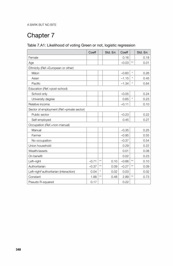
Chapter 7Table 7.A1: Likelihood of voting Green or not, logistic regression
Coeff Std. Err. Coeff Std. Err.Female 0.16 0.18Age –0.03 ** 0.01Ethnicity (Ref.=European or other) Māori –0.60 * 0.26 Asian –1.15 * 0.45 Pacific –1.34 * 0.64Education (Ref.=post-school) School only –0.05 0.24 university degree 0.65 * 0.23Relative income –0.11 0.10Sector of employment (Ref.=private sector) Public sector –0.23 0.22 Self-employed 0.45 0.27occupation (Ref.=non-manual) Manual –0.35 0.25 Farmer –0.95 0.55 No occupation –0.37 0.54union household 0.29 0.22wealth/assets 0.01 0.08on benefit 0.02 0.23Left–right –0.71 ** 0.10 –0.66 ** 0.10Authoritarian –0.37 ** 0.09 –0.27 ** 0.09Left–right*authoritarian (interaction) 0.04 * 0.02 0.03 0.02Constant 1 .88 ** 0.48 2.89 ** 0.73Pseudo R-squared 0.17 0.22

349
APPENdIxTa
ble
7.A2
: Spl
it vo
ting,
201
4 el
ectio
n (to
tal p
erce
ntag
es)
Elec
tora
te v
ote
Party
vot
eAC
TC
onse
rv-
ativ
eG
reen
Inte
rnet
- M
ANA
Labo
urM
āori
Nat
iona
lN
Z Fi
rst
Uni
ted
Futu
reO
ther
sIn
depe
nden
ts
& no
n-lis
t pa
rties
Can
dida
te
info
rmal
sPa
rty
vote
on
ly
Party
vo
te
ACT
0.18
0.03
0.02
0.00
0.09
0.00
0.32
0.01
0.00
0.00
0.00
0.02
0.01
0.69
Cons
erva
tive
0.03
1.59
0.06
0.01
0.40
0.01
1 .66
0.07
0.02
0.03
0.01
0.03
0.04
3.96
Gre
en P
arty
0.03
0.09
3.69
0.18
5.05
0.15
0.91
0.13
0.02
0.08
0.03
0.08
0.21
10.6
5In
tern
et-M
ANA
0.01
0.02
0.16
0.60
0.39
0.05
0.05
0.02
0.00
0.03
0.01
0.01
0.07
1.41
Labo
ur P
arty
0.04
0.20
1 .31
0.40
20.5
80.
320.
790.
360.
040.
100.
030.
220.
6425
.02
Māo
ri Pa
rty0.
000.
010.
060.
090.
260.
660.
140.
020.
000.
010.
000.
020.
051.
32Na
tiona
l Par
ty0.
801.
040.
890.
062.
790.
2839
.00
0.47
0.47
0.18
0.05
0.33
0.49
46.8
3NZ
Firs
t 0.
050.
340.
530.
163.
230.
231.
601.
910.
020.
150.
050.
200.
158.
62un
ited
Futu
re0.
000.
010.
020.
000.
050.
000.
100.
010.
020.
000.
000.
000.
000.
22o
ther
s0.
010.
030.
120.
030.
210.
030.
150.
040.
000.
150.
010.
020.
030.
84Pa
rty In
form
als0.
000.
010.
010.
010.
120.
010.
050.
010.
000.
000.
000.
210.
010.
45El
ecto
rate
vot
e1.
153.
366.
861.
5433
.16
1.74
44.7
73.
040.
610.
720.
201.
151.
7010
0.00
Note
: oth
ers
are
ACT
New
Zea
land,
Aot
earo
a Le
galis
e Ca
nnab
is Pa
rty, B
an10
80, d
emoc
rats
for S
ocial
Cre
dit,
Focu
s Ne
w Z
ealan
d, N
Z In
depe
nden
t Co
alitio
n, T
he C
ivilia
n Pa
rty.
Sour
ce: E
lecto
ral C
omm
issio
n 20
17 (R
ecalc
ulat
ed fr
om o
rigin
al so
urce
).

A BARk BuT No BITE
350
Chapter 8Table 8.A1: Social groups and authoritarian–libertarianism: Ordinary least squares regression
Coeff r.s.e.Female –0.10 * 0.05Age 0.00 0.00(European)Māori 0.61 ** 0.07Pasifika 0.44 * 0.19Asian 0.69 ** 0.11(Post-school qualification)School only 0.14 ** 0.06university –0.38 ** 0.07Relative income –0.07 * 0.03(Private sector wage/salary)Public –0.07 0.06Self-employed 0.03 0.07(Non-manual household)Manual 0.09 0.06Farmer –0.07 0.13No occupation –0.20 0.17union household –0.17 * 0.07Assets scale –0.05 * 0.02on benefit –0.12 0.07Church attendance 0.17 * 0.07urban –0.12 * 0.05Constant 0.35 * 0.15R-squared 0.14
Table 8.A2: Social groups and attitudes to immigration: Ordinary least squares regression
Coeff r.s.e. Coeff r.s.e.Female –0.080 0.052 –0.08 0.05Age 0.004 * 0.002 0.00 0.00(European)Māori –0.335 ** 0.094 –0.10 0.10Pasifika 0.472 ** 0.111 0.29 0.16Asian 0.206 0.141 0.47 ** 0.12

351
APPENdIx
Coeff r.s.e. Coeff r.s.e.(Post-school qualification)School only –0.123 * 0.061 –0.07 0.06university 0.179 * 0.071 0.09 0.07Relative income 0.182 ** 0.027 0.14 ** 0.03(Private sector wage/salary)Public 0.084 0.067 0.06 0.06Self-employed 0.053 0.066 0.04 0.07(Non-manual household)Manual –0.025 0.064 0.00 0.06Farmer 0.005 0.127 0.03 0.13No occupation 0.131 0.140 0.14 0.15union household –0.104 0.068 –0.11 0.07Assets scale 0.014 0.025 0.00 0.02on benefit 0.113 0.066 0.11 0.06Married –0.111 0.057 –0.10 0.06Church attendance 0.160 * 0.071 0.19 * 0.07New Zealand born –0.27 ** 0.07Better in 10 years –0.05 * 0.02Can find job 0.07 ** 0.02Fear of income loss 0.00 0.02Economy last year 0.16 ** 0.03Inequality –0.03 0.11Left–right –0.08 ** 0.01Authoritarian–libertarian –0.04 ** 0.01Constant 1.824 ** 0.143 2.88 ** 0.21R-squared 0.10 0.16N 2,727 2,727
Note: Those most in favour 5, those most against 1.
Table 8.A3: Social groups and attitudes to abortion: Ordinary least squares regression
Coeff r.s.e. Coeff r.s.e.Female –0.15 * 0.07 –0.13 * 0.06Age 0.00 * 0.00 0.00 * 0.00(European)Māori 0.50 ** 0.13 0.39 ** 0.12Asian 0.66 ** 0.16 0.56 ** 0.16Pasifika 0.58 * 0.25 0.52 * 0.25

A BARk BuT No BITE
352
Coeff r.s.e. Coeff r.s.e.(Post-school qualification)School only 0.14 0.08 0.11 0.08university –0.26 ** 0.08 –0.18 ** 0.08Relative income –0.06 0.04 –0.06 0.04(Private sector wage/salary)Public 0.01 0.09 0.03 0.09Self-employed 0.09 0.10 0.08 0.10(Non-manual household)Manual 0.11 0.08 0.10 0.08Farmer –0.06 0.15 –0.07 0.16No occupation 0.14 0.17 0.15 0.17union household –0.16 0.08 –0.11 0.08Assets scale 0.01 0.03 0.02 0.03on benefit 0.27 ** 0.09 0.29 ** 0.09Married 0.04 0.07 0.02 0.07Church attendance 1.98 ** 0.10 1.95 ** 0.10Inequality –0.14 0.13Left–right 0.02 0.02Authoritarian–libertarian 0.08 ** 0.02Constant 1 .78 ** 0.19 1 .31 ** 0.24R-squared 0.29 0.30
Table 8.A4: New Zealand First vote choice models
Coeff r.s.e.Female –0.473 * 0.215Age 0.005 0.008(European)Māori –0.045 0.389Asian 0.000 0.691(Post-school qualification)School only –0.146 0.230university 0.056 0.308Relative income –0.039 0.123(Private sector wage/salary)Public 0.054 0.249Self-employed –0.544 0.282(Non-manual household)Manual –0.141 0.245Farmer –0.416 0.599
353
APPENdIx
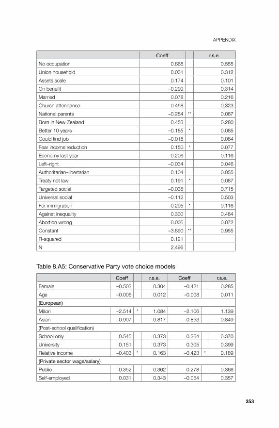
Coeff r.s.e.No occupation 0.868 0.555union household 0.031 0.312Assets scale 0.174 0.101on benefit –0.299 0.314Married 0.078 0.216Church attendance 0.458 0.323National parents –0.284 ** 0.087Born in New Zealand 0.453 0.280Better 10 years –0.185 * 0.085Could find job –0.015 0.084Fear income reduction 0.150 * 0.077Economy last year –0.206 0.116Left–right –0.034 0.046Authoritarian–libertarian 0.104 0.055Treaty not law 0.191 * 0.087Targeted social –0.038 0.715universal social –0.112 0.503For immigration –0.295 * 0.116Against inequality 0.300 0.484Abortion wrong 0.005 0.072Constant –3.890 ** 0.955R-squared 0.121N 2,496
Table 8.A5: Conservative Party vote choice models
Coeff r.s.e. Coeff r.s.e.Female –0.503 0.304 –0.421 0.285Age –0.006 0.012 –0.008 0.011(European)Māori –2.514 * 1.084 –2.106 1.139Asian –0.907 0.817 –0.853 0.849(Post-school qualification)School only 0.545 0.373 0.364 0.370university 0.151 0.373 0.305 0.399Relative income –0.403 * 0.163 –0.423 * 0.189(Private sector wage/salary)Public 0.352 0.362 0.278 0.366Self-employed 0.031 0.343 –0.054 0.357

A BARk BuT No BITE
354
Coeff r.s.e. Coeff r.s.e.(Non-manual household)Manual –0.383 0.387 –0.286 0.403Farmer –0.679 0.577 –0.527 0.555No occupation –1.715 1.109 –1.925 1.228union household –0.243 0.435 –0.195 0.469Assets scale 0.287 0.180 0.189 0.188on benefit –0.493 0.487 –0.551 0.473Married 1.169 ** 0.429 1.034 * 0.429Church attendance 2.024 ** 0.314 1.527 ** 0.392National parents 0.181 0.097 0.132 0.096Born in New Zealand 0.140 0.370 0.189 0.386Left–right 0.124 0.066Authoritarian–libertarian –0.133 0.079Treaty not law 0.276 0.151Targeted social –1.744 1.321universal social –0.419 0.810For immigration –0.172 0.175Against inequality –0.090 0.690Abortion wrong 0.349 ** 0.120Constant –4.068 ** 0.855 –3.557 ** 1.370R-squared 0.143 0.19N 2,551 2,551
Table 8.A6: Liking or disliking the ACT Party
Coeff r.s.e. Coeff r.s.e.Female 0.28 * 0.12 0.43 ** 0.11Age –0.01 * 0.00 –0.01 0.00(European)Māori 0.32 0.19 0.35 0.19Pasifika 1.03 ** 0.34 0.74 * 0.31Asian 1.34 ** 0.36 0.96 ** 0.32(Post-school qualification)School only 0.10 0.14 0.01 0.13university –0.51 ** 0.16 –0.24 0.15Relative income 0.18 ** 0.06 –0.01 0.06(Private sector wage/salary)Public –0.30 * 0.15 –0.25 0.13Self-employed –0.29 0.18 –0.33 * 0.17(Non-manual household)Manual –0.03 0.14 0.06 0.14

355
APPENdIx
Coeff r.s.e. Coeff r.s.e.Farmer 0.11 0.29 0.07 0.30No occupation 0.47 0.43 0.39 0.35union household –0.61 ** 0.16 –0.32 * 0.15Assets scale 0.17 ** 0.06 0.10 * 0.05on benefit 0.00 0.15 0.00 0.14Married –0.23 0.13 –0.33 ** 0.12Church attendance 0.41 ** 0.15 0.17 0.17National parents 0.20 ** 0.04 0.07 0.04NZ born –0.24 0.14 –0.07 0.14urban–not urban –0.08 0.12 0.02 0.11Better 10 years 0.19 ** 0.05Could find job 0.00 0.05Fears income loss 0.03 0.05Economy last year 0.00 0.07Left–right 0.17 ** 0.03Authoritarian–libertarian 0.05 0.03Treaty 0.11 * 0.05universal social –1.25 ** 0.43Targeted social –0.30 0.34Immigration 0.22 ** 0.06Inequality –1.50 ** 0.24Abortion 0.14 ** 0.05Constant 3 .11 ** 0.39 2.91 0.62R-squared 0.089 0.206N 2,672 2,672
Chapter 10The Māori Electorate NZES dataThe 2014 NZES oversampled the Māori electorates, and within that young voters as well. The response rate for those freshly sampled (N=284) was 19.2 per cent. Another 263 Māori electorate respondents came from the 2011 panel that, overall, had a 61.7 per cent response rate from those responding in 2011. The full Māori electorate sample has an N of 547. Despite the low response rate, within expected margins of error it contained a good representation of the various groups of voters, although non-voters were under-represented. Findings are based on weighting to more accurately reflect the vote/non-vote distributions for the party and electorate votes.

A BARk BuT No BITE
356
Table 10.A1: Comparing candidate effects on the Labour vote: Māori electorate and the general electorate vote
Coeff r.s.e.Age –0.012 ** 0.003Female –0.110 0.111Parents Labour 0.396 ** 0.071Favours Labour candidate 2.930 ** 0.151Favours Māori Party candidate –0.686 * 0.306Labour MP incumbent 0.209 0.216Favours MANA candidate –0.785 0.433Labour Party most favoured 2.303 ** 0.191Māori electorate 0.162 0.222Labour candidate*Māori electorate (interaction) –1.482 ** 0.351Constant –1.754 ** 0.222 /lnsig2u –2.213 0.633sigma_u 0.331 0.105rho 0.032 0.020N (Clusters) 2,805 (71)
Note: This is a multilevel model with random effects, taking account of the clustering of the electorate-level data. The dependent variable is an electorate vote for Labour versus the rest. To make sure that the effects we identify are not due to deeper party preferences or to the advantages of incumbency, we control for the following: whether there is an incumbent Labour MP; whether or not people report that Labour is the party they most like; and preferences for other candidates. we also control for parental party preferences for Labour. By interacting a preference for the Labour candidate or not with Māori or general electorate, we therefore estimate the relative effects of candidate preferences in the two classes of electorate.

357
APPENdIxTa
ble
10.A
2: B
asel
ine
mod
el o
f vot
ing
in th
e M
āori
elec
tora
tes:
The
ele
ctor
ate
vote
(mul
tinom
ial l
ogis
tic re
gres
sion
)
Non
-vot
eG
reen
Māo
ri Pa
rty
MAN
AAg
e–0
.013
0.01
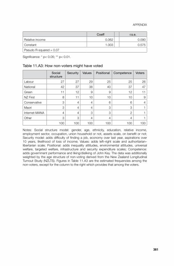
3–0
.007
0.02
10.
013
**0.
012
0.01
80.
014
Iwi c
onne
ctio
n–0
.770
*0.
444
0.19
50.
647
0.26
00.
454
0.64
20.
589
Spea
ks te
reo
0.23
90.
737
–1.0
441.
128
1.45
0**
0.59
91.
016
0.62
9Lo
w e
duca
tion
0.09
30.
409
–0.4
210.
568
–0.2
66*
0.39
4–0
.248
0.41
8ur
ban
–0.2
980.
390
1.19
4**
0.61
0–0
.478
0.42
6–0
.030
0.43
8M
anua
l hou
seho
ld0.
560
0.39
4–0
.295
0.67
30.
238
0.41
11.
078
**0.
426
Asse
ts s
cale
0.08
20.
167
–0.5
59**
0.25
30.
285
**0.
128
0.09
40.
162
Pare
nts
Labo
ur‡
0.01
70.
213
–0.6
24**
0.25
2–0
.145
0.22
4–0
.283
0.20
1Co
nsta
nt1.
114
*0.
629
–0.7
311.
090
–1.4
87**
0.63
6–2
.411
***0.
697
R-sq
uare
d0.
085
N44
8
Note
s: L
abou
r vot
e is
the
miss
ing
or re
sidua
l cat
egor
y in
the
mul
tinom
ial lo
git m
odel,
all o
ther
beh
avio
ur is
thus
mea
sure
d ag
ainst
a L
abou
r vot
e. N
ot v
otin
g is
indi
stin
guish
able
from
Lab
our v
otin
g, a
t lea
st in
term
s of
sta
tistic
al sig
nific
ance
.‡
This
varia
ble
mea
sure
s pa
rent
al pa
rtisa
nshi
p an
d ha
s a
scor
e of
2 w
hen
both
par
ents
vot
ed L
abou
r, on
e w
hen
one
of th
e pa
rent
s vo
ted
Labo
ur, a
nd z
ero
whe
n th
ere
is no
kno
wled
ge a
bout
par
enta
l par
tisan
ship
. Si
gnific
ance
: * p
< 0.
05; *
* p<
0.01
.

A BARk BuT No BITE
358
Tabl
e 10
.A3:
Bas
elin
e m
odel
of v
otin
g in
the
Māo
ri el
ecto
rate
s: T
he p
arty
vot
e (m
ultin
omia
l log
istic
regr
essi
on)
Non
-vot
eN
atio
nal
Gre
enN
Z Fi
rst
Māo
ri Pa
rtyM
ANA
Age
–0.0
150.
012
0.01
30.
015
–0.0
26*
0.01
30.
014
0.01
20.
019
0.01
40.
050
*0.
014
Iwi c
onne
ctio
n–1
.049
*0.
445
–0.7
880.
662
0.30
70.
555
–0.9
29*
0.50
40.
036
0.52
7–0
.098
0.73
0Sp
eaks
te re
o–0
.247
0.74
6–1
.551
1 .11
80.
591
0.70
3–0
.091
0.64
90.
429
0.65
71.
007
0.64
2Lo
w e
duca
tion
0.10
00.
404
0.78
70.
577
–0.4
320.
486
0.63
20.
446
–0.4
120.
393
–0.7
820.
493
urba
n0.
079
0.38
2–0
.184
0.66
60.
261
0.48
20.
368
0.43
3–0
.321
0.42
70.
761
0.48
4M
anua
l ho
useh
old
0.21
50.
400
–0.8
280.
660
–0.2
290.
490
–0.5
290.
478
0.63
80.
422
–0.0
450.
441
Asse
ts s
cale
0.32
9*
0.16
80.
652
**0.
218
0.42
8*
0.16
70.
461
*0.
184
0.47
8**
0.14
60.
110
0.24
4Pa
rent
s La
bour
‡0.
169
0.21
7–0
.436
0.27
50.
056
0.25
50.
110
0.24
8–0
.116
0.19
5–0
.147
0.26
0
Cons
tant
0.81
60.
612
–2.4
96**
0.79
7–1
.007
0.61
9–2
.211
**0.
777
–2.6
54**
0.75
7–3
.945
**0.
918
R-sq
uare
d0.
100
N51
1
Note
s: L
abou
r vot
e is
the
miss
ing
or re
sidua
l cat
egor
y in
the
mul
tinom
ial lo
git m
odel,
all o
ther
beh
avio
ur is
thus
mea
sure
d ag
ainst
a L
abou
r vot
e. N
ot v
otin
g is
indi
stin
guish
able
from
Lab
our v
otin
g, a
t lea
st in
term
s of
sta
tistic
al sig
nific
ance
. ‡
This
varia
ble
mea
sure
s pa
rent
al pa
rtisa
nshi
p an
d ha
s a
scor
e of
2 w
hen
both
par
ents
vot
ed L
abou
r, on
e w
hen
one
of th
e pa
rent
s vo
ted
Labo
ur, a
nd z
ero
whe
n th
ere
is no
kno
wled
ge a
bout
par
enta
l par
tisan
ship
. Si
gnific
ance
: * p
< 0.
05; *
* p<
0.01
.

359
APPENdIxTa
ble
10.A
4: D
imen
sion
al m
odel
of v
otin
g in
the
Māo
ri el
ecto
rate
s: T
he p
arty
vot
e
Non
-vot
eN
atio
nal
Gre
enN
Z Fi
rst
Māo
riM
ANA
Age
–0.0
230.
013
0.01
00.
018
–0.0
43**
0.01
50.
004
0.01
30.
014
0.01
60.
047
**0.
017
Iwi c
onne
ctio
n–0
.738
0.46
7–0
.389
0.70
10.
627
0.62
8–0
.687
0.54
0–0
.211
0.60
6–0
.084
0.73
6Sp
eaks
te re
o0.
125
0.94
1–1
.186
1 .31
60.
044
0.76
10.
257
0.69
90.
483
0.84
60.
146
0.78
6Lo
w e
duca
tion
0.17
30.
426
0.82
60.
609
–0.1
740.
478
0.93
00.
498
–0.2
760.
452
–1.1
010.
605
urba
n–0
.061
0.40
6–0
.525
0.76
00.
445
0.43
80.
265
0.46
7–0
.142
0.45
50.
786
0.60
6M
anua
l ho
useh
old
0.28
30.
420
–0.8
200.
738
–0.2
030.
450
–0.6
610.
499
0.94
50.
495
–0.2
390.
560
Asse
ts s
cale
0.39
1*
0.17
60.
683
**0.
253
0.54
1**
0.18
50.
526
**0.
200
0.50
3**
0.16
40.
311
0.26
8Pa
rent
s La
bour
0.15
00.
222
–0.3
990.
329
–0.0
450.
242
0.06
80.
249
–0.0
640.
211
–0.4
960.
334
Likes
Lab
our c
.†–1
.799
**0.
488
–1.3
01**
0.64
2–1
.184
*0.
506
–2.1
24**
0.55
0–0
.824
0.56
8–2
.231
*1.
007
Like
s M
ANA
c.–0
.292
0.75
4–1
4.42
9*
0.85
21.
062
0.79
6–1
.042
0.84
3–2
.446
*1.
219
2.85
7**
0.82
6Li
kes
Māo
ri c.
–0.3
240.
616
–0.5
930.
792
–0.3
200.
644
–0.6
340.
620
1.44
7**
0.47
6–0
.532
0.84
8In
cum
b M
RIM
P–1
.401
*0.
560
–1.7
45*
0.81
9–0
.020
0.66
0–1
.382
*0.
592
0.22
50.
478
–1.2
370.
770
Trea
ty–0
.579
0.62
7–1
.834
**0.
691
–0.4
870.
717
–0.5
620.
730
0.50
20.
655
0.64
70.
997
Ineq
uality
–1.9
86*
0.83
3–2
.351
*0.
954
1.59
91.
169
0.34
30.
928
0.11
00.
895
–0.1
001.
330
Cons
tant
4.21
1**
0.96
61.
791
1.17
4–0
.232
1.43
6–0
.471
1 .17
8–2
.676
*1.
144
–3.2
621.
730
R-sq
uare
d.2
0N
511
Sign
ifican
ce: *
p<
0.05
; ** p
< 0.
01.
† c. =
can
dida
te.

A BARk BuT No BITE
360
Chapter 11Regression Model, Figure 11.3Data for the figure is estimated from a logistic regression of vote/not vote against age, female/male, Māori on Māori roll, Māori on general roll (with non-Māori on the general roll as a residual category). Gender and the two variables are also interacted with the age variable, which is continuous, using the mid-point within five-year bands.
Table 11.A1: Vote/not vote by age, gender, Māori and electorate
Voted or not Coeff Linear Std. ErrFemale 0.530 ** 0.079Age 0.032 ** 0.001Māori electorate –0.676 ** 0.130Māori on general roll –0.366 * 0.148Residual: non-MāoriInteractions with ageFemale –0.009 ** 0.002Māori electorate –0.001 0.003Māori on general roll 0.003 0.003Constant –0.352 ** 0.059Pseudo R-squared = 0.48N = 29,989
Significance: * p< 0.05; ** p< 0.01. Source: vowles 2015b.
Table 11.A2: Non-voting and social structure, 2014 election
Coeff r.s.e.Female 0.039 0.187Age –0.041 ** 0.010Assets scale –0.479 * 0.208Age*assets (interaction) 0.008 * 0.004(European) Māori 0.548 * 0.238 Asian 0.933 * 0.379 Pasifika 0.340 0.449(Post-school qualification) School only –0.225 0.212 university –0.859 ** 0.294
361
APPENdIx
Coeff r.s.e.Relative income 0.062 0.090Constant 1.003 0.575Pseudo R-squared = 0.07
Significance: * p< 0.05; ** p< 0.01.
Table 11.A3: How non-voters might have voted
Social structure
Security Values Positional Competence Voters
Labour 27 27 29 25 25 26National 42 37 38 40 37 47Green 11 12 9 9 12 11NZ First 8 11 10 10 10 9Conservative 3 4 4 6 6 4Maori 3 4 4 3 3 1Internet-MANA 4 4 3 3 2 1other 3 3 4 4 4 1
100 100 100 100 100 100
Notes: Social structure model: gender, age, ethnicity, education, relative income, employment sector, occupation, union household or not, assets scale, on benefit or not; Security model: adds difficulty of finding a job, economy over last year, aspirations over 10 years, likelihood of loss of income; values: adds left–right scale and authoritarian–libertarian scale; Positional: adds inequality attitudes, environmental attitudes, universal welfare, targeted welfare, infrastructure and security expenditure scales; Competence: adds government performance and liking/disliking of John key. The data was additionally weighted by the age structure of non-voting derived from the New Zealand Longitudinal Turnout Study (NZLTS). Figures in Table 11.A3 are the estimated frequencies among the non-voters, except for the column to the right which provides that among the voters.

This text is taken from A Bark But No Bite: Inequality and the 2014 New Zealand General Election, by Jack Vowles, Hilde Coffé and Jennifer
Curtin, published 2017 by ANU Press, The Australian National University, Canberra, Australia.