Application Note

Tang Resonator

Application Note: Tang Resonator Version 8.6/PC Part Number 30-090-101 Jan 2010 © Copyright IntelliSense Software Corporation 2004, 2005, 2006, 2007, 2008, 2009, 2010 All Rights Reserved. Printed in the United States of America This manual and the software described within it are the copyright of IntelliSense Software Corporation, with all rights reserved. Restricted Rights Legend Under the copyright laws, neither this manual nor the software that it describes may be copied, in whole or in part, without the written consent of IntelliSense Software Corporation. Use, duplication or disclosure of the Programs is subject to restrictions stated in your software license agreement with IntelliSense Software Corporation. Although due effort has been made to present clear and accurate information, IntelliSense Software Corporation disclaims all warranties with respect to the software or manual, including without limitation warranties of merchantability and fitness for a particular purpose, either expressed or implied. The information in this documentation is subject to change without notice. In no event will IntelliSense Software Corporation be liable for direct, indirect, special, incidental, or consequential damages resulting from use of the software or the documentation. IntelliSuite™, SYNPLE, CleanRoom, Blueprint, Fastfield Multiphysics, Hexpresso, TEM, IntelliMask, IntelliMask Pro, MEMS-Synth, 3DBuilder, IntelliFAB, FABViewer, WaveRunner, EDALinker, are trademarks of IntelliSense Software Corporation. Windows NT, Windows 2000, Windows XP, Vista and Windows 7 are trademarks of Microsoft Corporation. Patent Number 6,116,766: Fabrication Based Computer Aided Design System Using Virtual Fabrication Techniques Patent Number 6,157,900: Knowledge Based System and Method for Determining Material Properties from Fabrication and Operating Parameters

Table of Contents 1. Introduction 1

1.1. Background 1

2. Design Exploration 3

2.1. Frequency Analysis 4

2.2. DC Analysis 10

2.3. 3D Visualization of SYNPLE Model 12

2.4. Mask Extraction from SYNPLE 14

3. Process Validation/Visualization 15

3.1. Layout 15

3.2. Process Development with IntelliFab 15

3.3. Visualization in FabViewer 18

4. Extraction 20

4.1. Creating the Model in 3D Builder 20

4.2. Thermoelectromechanical Analysis 22

4.2.1 Setting up the model 22

4.2.2 Frequency Analysis 26

4.2.3 Static Analysis 29

4.3. System Model Extraction 33

4.3.1 What is System Model Extraction? 33

4.4. Extracting the Macromodel 35

5. Final Verification 41

5.1. Loading the Macromodel 41

5.2. Connecting Macromodel to a Circuit 43

5.3. Benchmarks 45

5.3.1 Effects of Ambient Pressure 45

5.3.2 DC Voltage vs. Displacement 48

6. Summary 49

1

1. Introduction In this application note, we will discuss the design of a resonator from initial system-level design exploration, through fabrication processing and device-level analysis, to macromodel extraction and verification. We will analyze the resonator we have developed and discuss the benefits of IntelliSuite, a complete Computer Aided Design (CAD) software package offered by IntelliSense, when it comes to MEMS-based resonator design. We will begin the design exploration in SYNPLE, the system-level simulator. Analyses can be performed very quickly in this tool, making it ideal for the initial design stages. We will then discuss the layout and process development of the device. From the mask layout we will automatically generate a 3D meshed model to be used for finite element analysis. After running simulations in the analysis module, we will extract a macromodel to be connected to a circuit and used for verification in SYNPLE. 1.1. Background Recent advances in fabrication and packaging technologies have allowed for the development of small, high-quality, cost-effective MEMS resonators. Resonators are now an important sector of the MEMS market, with a large potential for growth in the wireless communications and inertial sensing industries. This resonator design discussed in this application note was developed by Dr. William C. Tang, currently of UC-Irvine. A model of the resonator is shown in the figure below.

Figure 1: Resonator Model

One comb drive is used to drive the resonator, and a double-sided single-folded beam structure is used as a spring. The second comb drive is used to sense the displacement of the device. Shown below is a partial SEM micrograph of a Tang resonator.

2

Figure 2: Tang Resonator

3

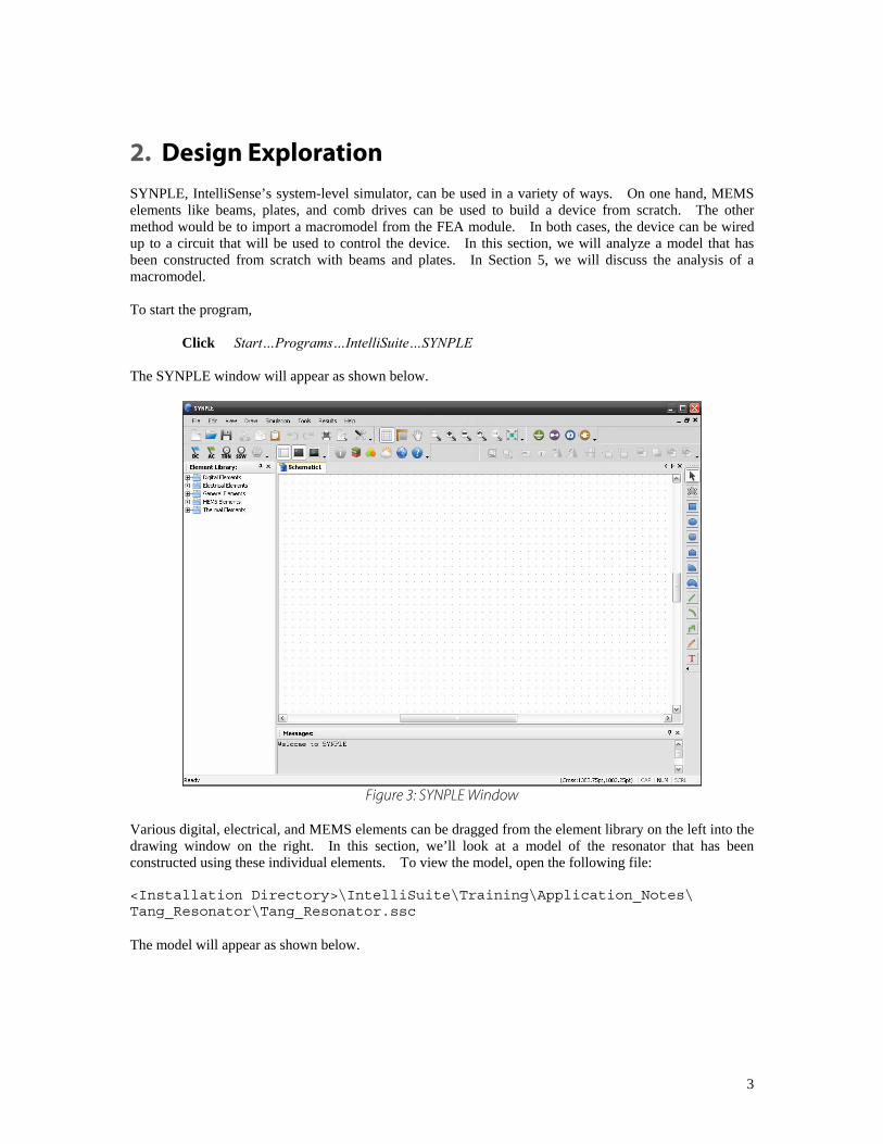
2. Design Exploration SYNPLE, IntelliSense’s system-level simulator, can be used in a variety of ways. On one hand, MEMS elements like beams, plates, and comb drives can be used to build a device from scratch. The other method would be to import a macromodel from the FEA module. In both cases, the device can be wired up to a circuit that will be used to control the device. In this section, we will analyze a model that has been constructed from scratch with beams and plates. In Section 5, we will discuss the analysis of a macromodel. To start the program, Click Start…Programs…IntelliSuite…SYNPLE The SYNPLE window will appear as shown below.

Figure 3: SYNPLE Window

Various digital, electrical, and MEMS elements can be dragged from the element library on the left into the drawing window on the right. In this section, we’ll look at a model of the resonator that has been constructed using these individual elements. To view the model, open the following file: <Installation Directory>\IntelliSuite\Training\Application_Notes\ Tang_Resonator\Tang_Resonator.ssc The model will appear as shown below.

4

Figure 4 Resonator Model in SYNPLE

Double click on any of the elements to view their individual parameters. 2.1. Frequency Analysis When you have finished examining the elements, Click Simulation…AC Analysis For the AC simulation, we will examine the device response to a frequency sweep from 1000 Hz to 1 MHz. The simulation settings are already set. To view the settings, Click Frequency Sweep

5

Figure 5 Frequency Sweep Selection and Settings

You will see the frequency range we are analyzing. To return to the simulation settings window, click OK. Under the Signals tab, you will see that the x- and y-displacement of the resonator will be observed. The settings in the Convergence Setup tab should be left on the defaults. To run the AC simulation, Click OK After about two minutes, a notification will appear in the message window informing you of the location of the simulation results. The Plot Manager window will also appear and will allow you to view a 2D graph of any of the output signals.

6

Figure 6 Feedback and Signal Manager Windows

Click mag_of_Y_ac

Click Open in Waverunner

Waverunner module will launch automatically. This module is new postprocessor of IntelliSuite, especially for MEMS, Analog, mixed signal waveform management.

Figure 7 Waverunner window

Click Chart… Import Data Source

Find the file “Tang_resonator.ac.dat”

Click Open

7

Click Add Chart

Figure 8 Select signal to display

Click Y_ac Click OK

The plot will appear as below:

Figure 9 AC Results

If you want to view the graph on a logarithmic scale, double click on the axes and the axis property editor window will appear.

8

Figure 10 Chart Information Dialog

Click Axes Click Y

Figure 11 axis options

Click Axis Options Select Log…Scale

9

Figure 12 logarithmic axis

The magnitude curve using logarithmic axes are shown below.

Figure 13 Magnitude Plot

To export the data to Excel or a text editor

Click Chart…Show Data

10

Figure 14 data window

Select and Copy to copy the data to the clipboard. You should notice that the resonant frequency is 34.4 kHz. 2.2. DC Analysis Open the following file: <Installation Directory>\IntelliSuite\Training\Application_Notes\ Tang_Resonator\Tang_Resonator_DC.ssc The model will appear as shown below.

11

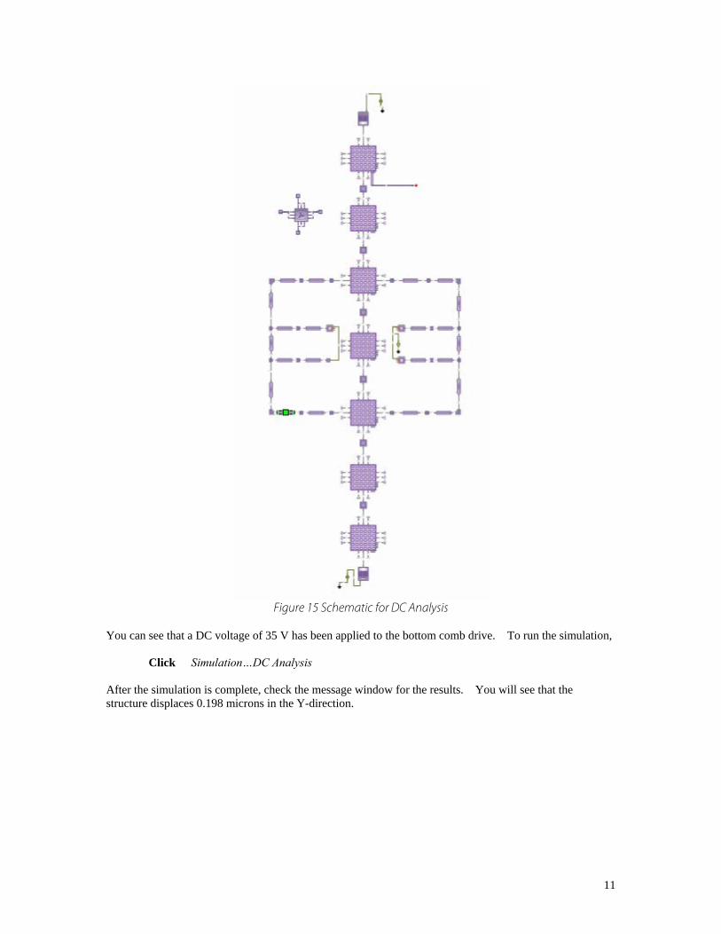
Figure 15 Schematic for DC Analysis

You can see that a DC voltage of 35 V has been applied to the bottom comb drive. To run the simulation, Click Simulation…DC Analysis After the simulation is complete, check the message window for the results. You will see that the structure displaces 0.198 microns in the Y-direction.

12

2.3. 3D Visualization of SYNPLE Model Results from a simulation in SYNPLE can be visualized in 3D. First, run the simulation again. Click Simulation…DC Analysis We will need results from all of the output signals to get an accurate 3D visualization. Select All Nodes under the Signals tab in the DC Simulation dialog.

Figure 16 DC Simulation Dialog

Click OK to run the simulation. After the simulation is complete, select MEMS 3D Visualization in the Results menu. If you don’t see this option, you need to reset your toolbar.

Click View…Preference…Customize or Click Reset… in the dialog box that appears. MEMS 3D Visualization should now appear as an option in the Results menu.

13

Figure 17 3D Visualization in Results Menu

IntelliSense’s post-processing module VisualEase will open with the 3D visualization of the device. Choose Displacement Y under the Variable box to view the y-displacement.

Figure 18 Resonator in VisualEase

14

2.4. Mask Extraction from SYNPLE Mask layouts can be extracted from your SYNPLE schematic. Select Synthesize Mask Layout in Blueprint from the Synthesis menu as shown in the figure below.

Figure 19 Synthesis Menu

Blueprint will automatically open with a mask layout for the structure.

Figure 20 Resonator Layout in Blueprint

15

3. Process Validation/Visualization There are two ways to build a model in IntelliSuite. A model based on the layout and actual fabrication processes can be constructed in IntelliFab and visualized in FabViewer. In 3D Builder, a user can generate a meshed 3D model of a device without worrying about the device processing. The first method will be discussed in this section, and the creation of a model in 3D Builder will be discussed in Section 4. 3.1. Layout The first step in building the resonator model is to generate the layout for the device. In Figure 21 you will see the layout used for the resonator.

Figure 21 Resonator Layout

To view the mask, you must run IntelliMask. Click Start…Programs…IntelliSuite…Blueprint Once you have started Blueprint you can open the mask. Click File…Open. You must select the file from: <Installation Directory>\IntelliSuite\Training\ 3DBuilder\Non-Manhattan_Isotropic\MUMPS\TangResonator.msk When you are finished inspecting the mask, exit the software. Click File…Exit. 3.2. Process Development with IntelliFab Once the layout is designed, the process must be developed. This is done using IntelliFab.

16

Click Start…Programs…IntelliSuite…IntelliFab. The IntelliFab window will appear. The database on the left contains all of the available process steps. Double-clicking on a process step will add it to the process flow on the right.

Figure 22 IntelliFab window

To view the resonator process flow that uses the MUMPs template, Click File…Open Fab… Select the file from the following location: <Installation Directory>\IntelliSuite\ Training\FabViewer\TangResonator\MUMPS_with_release_holes.fab. A setup window will appear where you can select the mask file and set the die size. Leave everything as is and click OK. The process flow will appear as shown below.

17

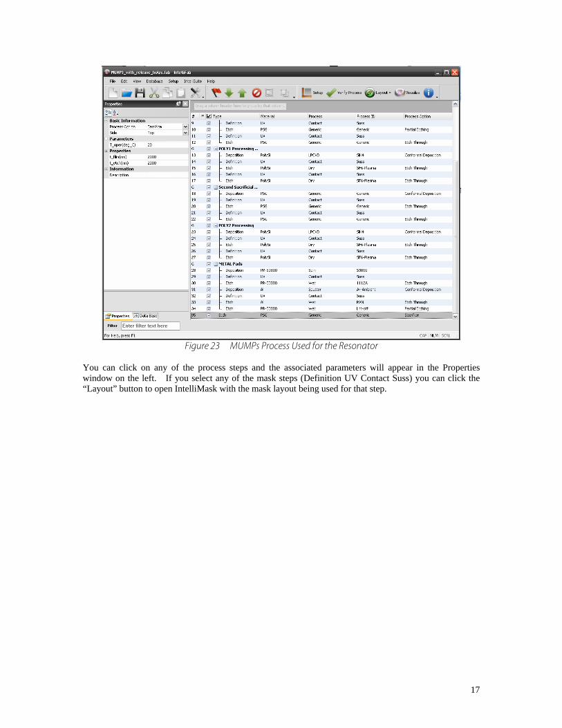
Figure 23 MUMPs Process Used for the Resonator

You can click on any of the process steps and the associated parameters will appear in the Properties window on the left. If you select any of the mask steps (Definition UV Contact Suss) you can click the “Layout” button to open IntelliMask with the mask layout being used for that step.

18

3.3. Visualization in FabViewer Once the process has been fully developed, the device can be visualized in FabViewer. Click IntelliSuite…Visualize in FabViewer FabViewer will open as shown below.

Figure 24 FabViewer Window

Click Setup…Resolution The resolution setup window will appear as below. Here you can input scaling factors for both the surface layers and the substrate. You can also select from a list of preset resolution values or input your own resolution settings. Set the resolution to Best as shown below.

19

Figure 25 Resolution settings

To view a simulation of the process and the resulting device, click the play button at the top of the screen. The figure below shows the final structure when the resolution is set to “Best”. The simulation will take about 5 minutes to run at this resolution setting.

Figure 26 Resonator Model in FabViewer

20

4. Extraction

4.1. Creating the Model in 3D Builder Building a model based on a process flow in IntelliFab (discussed in Section 3) is one way to create a model in IntelliSuite. The second method uses a program called 3D Builder to generate a meshed 3D model of a device based solely on the mask layout. The benefit of the second method is that it allows the user to forgo the process development part of MEMS design and skip straight to device level analysis, leaving process development to later. To open the program, Click Start…Programs…IntelliSuite…3D Builder. The 3D Builder window will appear. Select Automesh from mask layout in the Mesh drop-down menu.

Figure 27 Automeshing in 3D Builder

In the dialog box that appears, Click Browse… Select the following file: <Installation Directory>\IntelliSuite\Training 3DBuilder\Non-Manhattan_Isotropic\MUMPS\TangResonator.msk Click the Advanced Setup button. This will bring up a dialog box where you can choose which process steps to include.

21

Figure 28 Advanced Layer Setup

This particular device will be generated based on the MUMPS process. Leave all of the boxes checked, and click OK to return to the previous dialog box. Leave the maximum mesh size at 30 um and click OK in the Meshing Type dialog box. The program will then begin creating the automeshed structure.

Figure 29 Automeshed structure

22

For a better view of the structure, click inside the 3D window, then select View…Define View Z Scaling. Set the Z Scale Factor to 5. Open the following file: <Installation Directory>\IntelliSuite\Training\Application_Notes\ Tang_Resonator\Tang_Resonator.solid This structure is the same as the automeshed structure you just created, but the comb drives have been set as different entities. This will be necessary for applying voltage loads in the finite element analysis tool. To send the structure to the finite element analysis module, Click File…Export to Analysis Module… Click Continue without Check and select the ThermoElectroMechanical analysis module. Save the analysis file, making sure not to use spaces in the file or folder names. 4.2. Thermoelectromechanical Analysis The ThermoElectroMechanical Analysis Module (TEM) is the device-level finite element analysis application developed by IntelliSense. This module allows you to incorporate material properties, loads, and boundaries to fully analyze a device in the static, frequency, and dynamic domains. One additional feature that is completely unique to IntelliSuite’s TEM is the ability to create N-DOF system models from finite element models that can be imported into a system level simulator like SYNPLE. These models retain the accuracy of their finite element-based models, but can be quickly simulated under multiple loading conditions in the system-level solver. Another capability this allows is the ability to co-simulate your CMOS control circuitry with your finite element-based MEMS device. This is a very powerful capability only offered by IntelliSense that allows our users to fully develop their device from layout through processing and device level development all the way to the full integration of the MEMS device with their circuit. 4.2.1 Setting up the model The Export to Analysis Module function in 3D Builder will automatically open the model in the TEM module.

23

Figure 30 Resonator in TEM Module

To set the Z scaling factor, Click View…Zoom…Define Set the Zoom Factor in the z-direction to 5. The first step in the TEM module is to choose a simulation setting and check the material properties. Click Simulation…Simulation Setting. The window shown in Figure 31 will appear. In this window you will find all of the simulation types and their respective options.

24

Figure 31 Simulation Setting Window

In the first simulation we will run is a natural frequency analysis, so set the Calculation Type to Frequency, and the Analysis Type to Static Stress. Set the simulation to analyze the first 5 modes using small scale displacement theory, an undeformed start shape, and no piezomaterial. Once we have the simulation set, we can work on our material properties, loads, and boundaries. Click Material…Check/Modify. Select the entity that includes the beams and comb drives and makes up the moving structure. The entity will turn red and the Material Properties dialog will appear.

25

Figure 32 Material Properties

You will find that this entity has the material properties of poly silicon. The material properties of the rest of the entities do not matter in this case because they will be used for electrostatic purposes only, none of them will move. Click OK to exit this dialog. Once we have verified the material properties, we need to apply the boundary conditions for the model. In this example, we will only use the Fixed boundary condition. Click Boundary…Selection Mode…Pick on Geometry Click Boundary…Fixed Select the faces shown in Figure 30. All fixed faces are displayed in red.

Figure 33 Fixed Faces displayed in red When you feel you have finished applying the fixed boundary conditions, check that they have all been applied.

26

Click Boundary…Selection Mode…Check Only. Click Boundary…Fixed. The software should go through a command prompt, and all of the fixed faces will appear in bright red. Note that you would have to select Boundary…Pick on Geometry before you could define any more boundary conditions. 4.2.2 Frequency Analysis Because we have already set up the simulation with the correct material properties and boundaries, the frequency analysis is easy to complete. Click Analysis…Start Frequency Analysis The frequency analysis will take 2-3 minutes. A command prompt similar to the one shown below will appear on the screen while the simulation is running.

Figure 34 Natural Frequency Results

When this window disappears, the simulation is complete. After the simulation, the results available to you will be the list of natural frequencies and animations of each mode shape. These can be found next to each other in the Result menu (Figure 35).

27

Figure 35 Natural Frequency Results

Click Result…Natural Frequency You will see the list of natural frequencies shown in Figure 36.

Figure 36 List of Natural Frequencies

Click OK to exit this dialog. If you want to view the animation of one of the natural frequencies,

28

Click Result…Mode Animation This will bring up a window that will ask you for the mode number of the natural frequency you want to animate and the scale factor.

Figure 37 Mode animation selection box

Select 2 for the mode number and 1 for the scale factor. When the mode animation begins, you will see the mass moving in the y-direction. This is the mode that we are interested in (Mode 1 corresponds to the movement of the mass in the z-direction). The natural frequency of mode 2 is 34744 Hz.

29

4.2.3 Static Analysis Close the frequency analysis model and open the following file: <Installation Directory>\IntelliSuite\Training\Application_Notes\ Tang_Resonator\TEM\Resonator_DC.save In the Model Explorer on the left, you will see that static voltage loads have been applied to the model (applied using the Voltage…Entity option under the Loads menu). Double-click on Voltage Entity 4 and you will see that a 35 V load has been applied to the top comb drive. The folded-beam structure and opposite comb drive have been set to 0 V.

Figure 38 Model Explorer

With all finite element solvers, a solution is more accurate with a more refined mesh. One thing that is special to IntelliSuite and its TEM is the ability to decouple the mechanical and electrostatic meshes. This allows the user to define where the important mechanical elements are and where the important electrostatic elements are. In this particular case, the important electrostatic elements are the comb drives. To refine the electrostatic mesh, Click Mesh…Group Surfaces for Elec_mesh…Group Surfaces The Group Mesh Dialog will appear. Fill in the values in Figure 36 and click OK.

30

Figure 39 Mesh Coordinates for Comb 1

Click Mesh…Group Surfaces for Elec_mesh…Group Surfaces Fill in the values in Figure 37 and click OK.

Figure 40 Mesh Coordinates for Comb 2

31

Click Mesh…Update Electrical Mesh The electrostatic mesh will appear as shown below.

Figure 41 Electrostatic Mesh

Click Simulation…Simulation Setting to view the simulation settings for this model.

Figure 42 Static Simulation Settings

32

The material properties and boundary conditions are the same as defined in the previous model. After you have finished examining the model, Click Analysis…Start Static Analysis When the command prompt disappears, the simulation is complete. To view the y-displacement results, Click Result…Displacement…Y The model will appear as shown below.

Figure 43 Y-Displacement Results

To view the displacement of a certain node, Click Result…Node Value Click the center of the proof mass, for example. You will see that the y-displacement is 0.199 microns. The value obtained earlier from SYNPLE is within 0.5% of this value. For more information on the comparison of static simulations in SYNPLE and TEM, see Section 5.3.2.

33

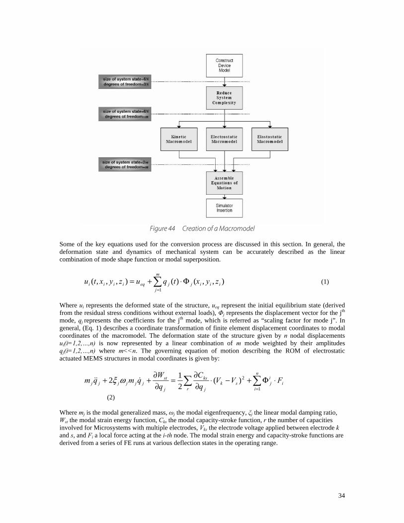
4.3. System Model Extraction 4.3.1 What is System Model Extraction? SME is a means by which a full three-dimensional meshed numerical model of a multi-conductor electromechanical device without dissipation can be converted into a reduced-order analytical macromodel. This can then be inserted as a black-box element into a mixed signal circuit simulator. This process is based upon the energy method approach, in that we construct analytical models for each of the energy domains of the system and determine all forces as gradients of the energy. The energy method approach has the advantage of making this process modular, enabling us to incorporate other energy domains into our models in the future. Another beneficial side effect of energy methods is that the models we construct are guaranteed to be energy conserving, because each of the stored energies is constructed as an analytical function, and all forces are computed directly from analytically computed gradients. The SME process also has the advantage of being able to be performed almost entirely automatically, requiring the designer only to construct the model, run a few full three-dimensional numerical computations, and set a few preferences a priori. Above all, this process has the ultimate benefit of constructing models that are computationally efficient, allowing their use in a dynamical simulator. Our first task is to reduce the degrees of freedom of the system. Rather than allow each node in a finite element model to be free to move in any direction, we constrain the motion of the system to a linear superposition of selected set of deformation shapes. This set will act as our basis set of motion. The positional state of the system will hence be reduced to a set of generalized coordinates, each coordinate being the scaling factor by which its corresponding basis shape will contribute. Next, we must construct analytical macromodels of each of the energy domains of the system. In the case of conservative capacitive electromechanical systems, these consist of the electrostatic, elastostatic, and kinetic energy domains. These macromodels will be analytical functions of the generalized coordinates. (As we will see in the section on Using Mode Shapes as a Basis Set, some of these energy domains will be determined as a byproduct of modal analysis, avoiding the need for explicit calculation.) We can then use Lagrangian mechanics to construct the equations of motion for the system in terms of its generalized coordinates. Finally, we can translate these equations of motion into an analog hardware description language, thereby constructing a black-box model of the electromechanical system that can be inserted into an analog circuit simulator. The figure below gives the Flow Chart for the conversion of an FEA model into an equivalent system level mode.

34

Figure 44 Creation of a Macromodel

Some of the key equations used for the conversion process are discussed in this section. In general, the deformation state and dynamics of mechanical system can be accurately described as the linear combination of mode shape function or modal superposition.

),,()(),,,(1

iii

m

jjjeqiiii zyxtquzyxtu ∑

=

Φ⋅+= (1)

Where ui represents the deformed state of the structure, ueq represent the initial equilibrium state (derived from the residual stress conditions without external loads), Φj represents the displacement vector for the jth

mode, qj represents the coefficients for the jth mode, which is referred as “scaling factor for mode j”. In general, (Eq. 1) describes a coordinate transformation of finite element displacement coordinates to modal coordinates of the macromodel. The deformation state of the structure given by n nodal displacements ui(i=1,2,…,n) is now represented by a linear combination of m mode weighted by their amplitudes qj(i=1,2,…,n) where m<<n. The governing equation of motion describing the ROM of electrostatic actuated MEMS structures in modal coordinates is given by:

i

n

i

ijsk

r j

ks

j

stjjjjjj FVV

qC

qW

qmqm ⋅Φ+−⋅∂∂

=∂∂

++ ∑∑=1

2)(212 &&& ωξ

(2) Where mj is the modal generalized mass, ωj the modal eigenfrequency, ξj the linear modal damping ratio, Wst the modal strain energy function, Cks the modal capacity-stroke function, r the number of capacities involved for Microsystems with multiple electrodes, Vks the electrode voltage applied between electrode k and s, and Fi a local force acting at the i-th node. The modal strain energy and capacity-stroke functions are derived from a series of FE runs at various deflection states in the operating range.

35

The modal superposition method is efficient since just one equation per mode and one equation per conductor is necessary to describe the coupled system entirely, which can be applied to both linear and nonlinear geometry. The modal superposition based reduced order modeling procedure includes the following steps:

• Determine the “Modal Contribution”. In this step, the software performs the standard electromechanical relaxation analysis and solves the initial deformed state (derived from the residual stress without external loads) and the final deformed state (with mechanical loads and applied voltages). Then use the QR factorization algorithm to determine the mode contribution for the deformed state.

• Calculate the relationship of “Strain Energy vs Modal amplitudes” for each mode. • Calculate the relationship of “Mutual capacitance vs Modal amplitudes”. • From step 2 and 3, the user will obtain ∂Wst(q)/∂qj and ∂C(q)/∂qj respectively.

. 4.4. Extracting the Macromodel The following procedure describes the steps to extract an electromechanical macromodel of the resonator.

Click Simulation…Simulation Setting

Set the simulation as shown in the figure below.

Figure 45 Modal Contribution Simulation Settings

36

Click OK To start the analysis, Click Analysis…Start Extract Macro Model Once the analysis is complete, Click Result…Macromodel…Modal Contribution This will show the contribution of each mode to the deformation of the device.

Figure 46 Modal Contribution

If you wanted to reduce the time necessary to complete the strain energy calculation (the next step), you could disable any of the modes by double-clicking on them. In this case we will use all five modes. Next, we will run the strain energy calculation.

Click Simulation…Simulation Setting Set the simulation as shown in the figure below.

37

Figure 47 Strain Energy Simulation Settings

Click OK To start the analysis, Click Analysis…Start Extract Macro Model Once the analysis is complete, Click Result…Macromodel…Strain Energy vs. Modal Amplitudes To show a plot of the strain energy vs. scaling factor for a particular mode, double-click on the mode number and click OK.

38

Figure 48 Strain Energy vs. Mode 1

Next, select the Mutual Capacitance vs. Modal Amplitudes button in the Simulation Settings window.

Figure 49 Capacitance Simulation Settings

39

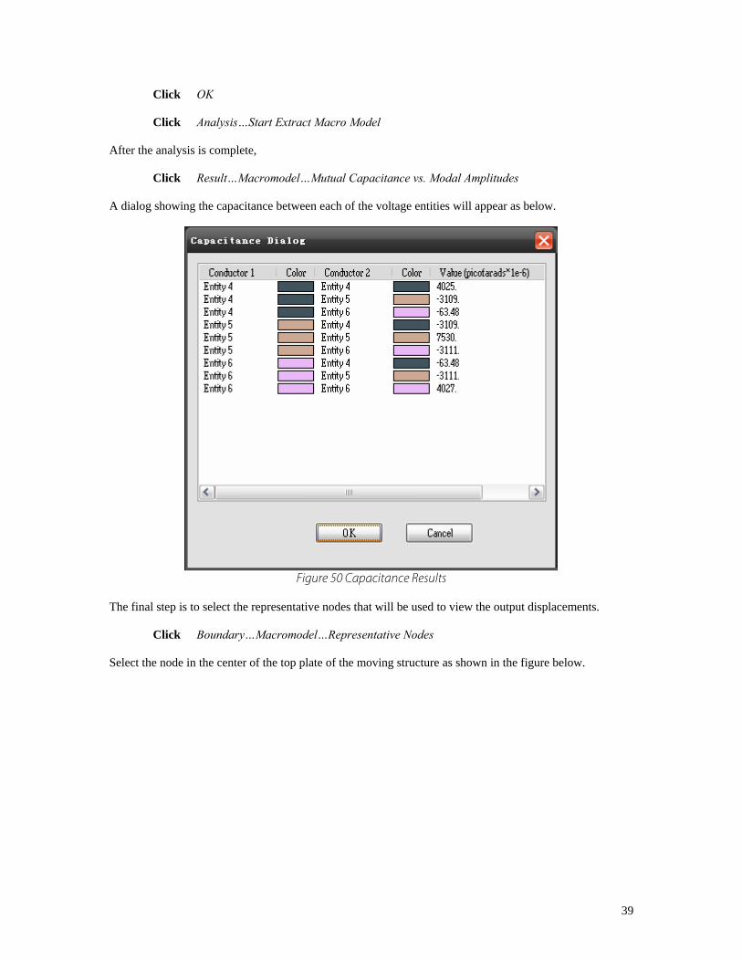
Click OK Click Analysis…Start Extract Macro Model After the analysis is complete, Click Result…Macromodel…Mutual Capacitance vs. Modal Amplitudes A dialog showing the capacitance between each of the voltage entities will appear as below.

Figure 50 Capacitance Results

The final step is to select the representative nodes that will be used to view the output displacements. Click Boundary…Macromodel…Representative Nodes Select the node in the center of the top plate of the moving structure as shown in the figure below.

40

Figure 51 Representative Node

When you have selected the representative nodes, the macromodel extraction is complete. Save the TEM file. Copy the “curr.macromodel,” “macromodel.out,” and “str.out” files from the active directory and place them in a new directory for use with SYNPLE. Be sure to move these files to a new folder, as they will be overwritten in the current directory if you run another simulation.

41

5. Final Verification Simulations, especially dynamic simulations, can take several hours to complete in the TEM module. Extracting a macromodel and running the simulation in SYNPLE can save a great deal of time without sacrificing the accuracy of the results. You will also be able to connect the macromodel to the circuitry that will be used to control the device. 5.1. Loading the Macromodel To open SYNPLE, Click Start…Programs…IntelliSuite…SYNPLE Click and drag the MEMS Devices…Macro-Model-I element from the element library on the left into the drawing window.

Figure 52 Schematic with Macro-Model Element

The next step is to link the macromodel element to the macromodel file we have extracted. Click on the Macro-Model element to highlight it.

Click Tools…Load ROM Macro-model To load the macromodel, you would need to find the location of your macromodel files, select the “curr.macmodel” file, and click Open. This will bring up a verification dialog box to let you know that the macromodel has been properly loaded and linked to the element. In this case, we will examine a schematic that has already been created. Open the following file:

42

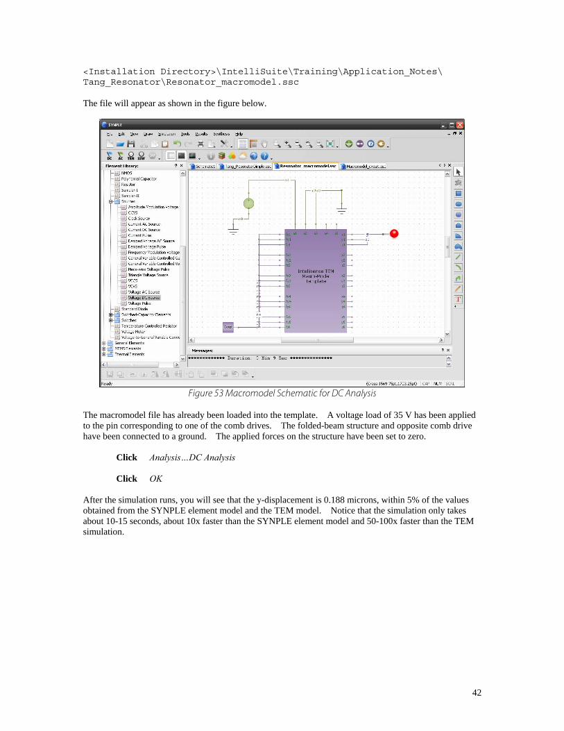
<Installation Directory>\IntelliSuite\Training\Application_Notes\ Tang_Resonator\Resonator_macromodel.ssc The file will appear as shown in the figure below.

Figure 53 Macromodel Schematic for DC Analysis

The macromodel file has already been loaded into the template. A voltage load of 35 V has been applied to the pin corresponding to one of the comb drives. The folded-beam structure and opposite comb drive have been connected to a ground. The applied forces on the structure have been set to zero.

Click Analysis…DC Analysis

Click OK After the simulation runs, you will see that the y-displacement is 0.188 microns, within 5% of the values obtained from the SYNPLE element model and the TEM model. Notice that the simulation only takes about 10-15 seconds, about 10x faster than the SYNPLE element model and 50-100x faster than the TEM simulation.

43

5.2. Connecting Macromodel to a Circuit Open the following file: <Installation Directory>\IntelliSuite\Training\Application_Notes\ Tang_Resonator\Macromodel_circuit.ssc The schematic will appear as shown below.

Figure 54 Macromodel and Circuit for AC Analysis

The folded beam structure has been connected to a DC voltage. An AC voltage has been attached to one comb drive, and the inverted signal has been attached to the other comb drive. The frequency of the AC source has been set to 35 kHz to activate mode 2. To run the simulation,

Click Analysis…AC Analysis

Click OK After the simulation runs, double click mag_of_y1_ac in the Plot Manager.

44

Figure 55 Plot Manager

This will bring up a plot of the AC response in the y-direction as shown below. Note that the axes in this curve have been set to Logarithmic Scale as discussed earlier in Section 2.1.

Figure 56 AC Response

Since mode 2 is being activated, this curve only shows the response corresponding to mode 2 and not any of the other modes. The peak occurs at 34.6 kHz, within 0.5% of the value from TEM.

45

5.3. Benchmarks 5.3.1 Effects of Ambient Pressure The quality factor for the resonator will be highly dependent upon the packaging pressure for the device. In this section we will observe how the AC response changes for different packaging pressures. The ambient parameter settings can be accessed through the Ambient Parameters button in the Managers toolbar.

Figure 57 Managers Toolbar

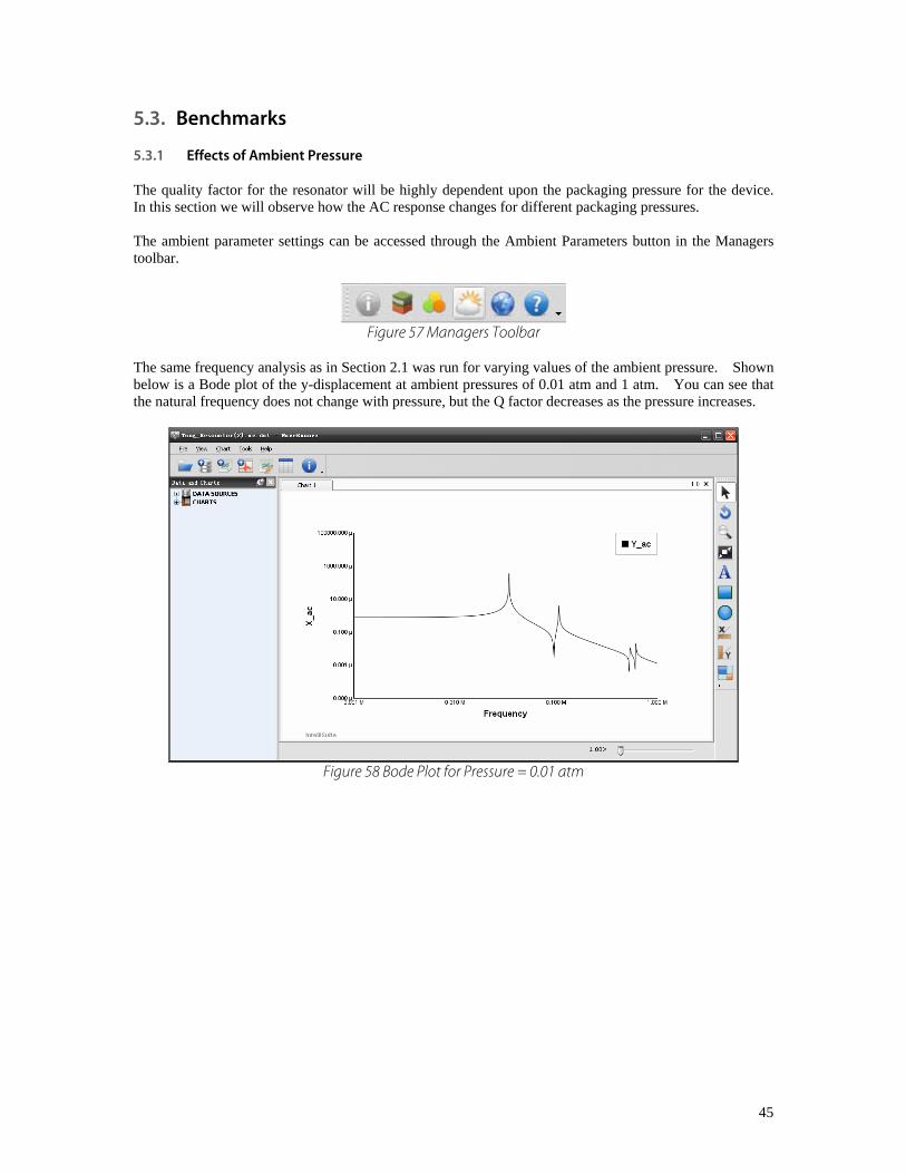
The same frequency analysis as in Section 2.1 was run for varying values of the ambient pressure. Shown below is a Bode plot of the y-displacement at ambient pressures of 0.01 atm and 1 atm. You can see that the natural frequency does not change with pressure, but the Q factor decreases as the pressure increases.

Figure 58 Bode Plot for Pressure = 0.01 atm

46

Figure 59 Bode Plot for Pressure = 1 atm

The results from SYNPLE were compared with an empirical model developed by Xia Zhang and William C. Tang. This model predicts the Q factor of such a resonator for various packaging pressures and is defined as

( ) ⎟⎟

⎠

⎞⎜⎜⎝

⎛+⎟

⎠⎞

⎜⎝⎛ +=

hdAd

dhA

lwAEQ c

cq

mδ

α

ρμ 1

/2

13

1

(1)

where μ is the effective viscosity of the ambient fluid, E is the Young’s modulus of the structure, ρ is the density, Am is the effective area, w and l are the width and length of the beams, α is an experimental scaling factor, Aq is the damping-related effective area, d is the air film thickness, h is the structure thickness, δ is the penetration depth, Ac is the area of comb finger overlap, and dc is the comb finger gap. The effective viscosity is calculated using the following equation:

10/788.02.021 nK

nn

stp

eKK −++=

μμ 2,

(2) where μstp is the viscosity of the fluid at standard temperature and pressure and Kn is the Knudsen number, given by

d

K nλ= .

(3)

λ is the mean free path and d is the air gap in this case. The Q factor obtained from SYNPLE was compared to Q obtained from Equation 1. The results are shown below.

47

0

100

200

300

400

500

600

700

0.001 0.01 0.1 1 10 100

Pressure (atm)

Q fa

ctor SYNPLE

Empirical

Figure 60 SYNPLE/Empirical Comparison

As you can see, the results from SYNPLE match up very well with the empirical predictions.

48

5.3.2 DC Voltage vs. Displacement Varying static voltages were placed on one of the comb drives in the SYNPLE element model, TEM finite element model, and SYNPLE macromodel. The displacement of the central mass was obtained from each of the models, and the results are plotted in the figure below.

0.00

0.05

0.10

0.15

0.20

0.25

0.30

0.35

0.40

0.45

0 10 20 30 40 50 60

Voltage (V)

Dis

plac

emen

t (um

)

TEMSYNPLEMacromodel

Figure 61 DC Voltage vs. Displacement

As you can see, the results from the three models match up almost exactly.

49

6. Summary In this application note we discussed the development of a Tang resonator from the initial design stages all the way through the design process to final verification and control circuitry integration. We first began the design exploration in SYNPLE. The capability to run simulations that are much faster than FEA simulations makes this a great tool for early design optimization. Furthermore, the 3D visualization and mask extraction features make it easy to jump right into the next stage of the design process. From a mask layout in IntelliMask and process flow in IntelliFab we were able to create a 3D model based on processing effects in FabViewer. We also used the automeshing feature in 3D Builder to create a 3D model from the mask layout with one click. From there the model was exported to the ThermoElectroMechanical Analysis model for a more in-depth analysis. We discussed how to set up the simulation and learned about IntelliSuite’s unique mesh refinement capabilities. The TEM uses Exposed Face Meshing methods to de-couple the mechanical and electrostatic meshes of devices, allowing users to perform mechanical mesh refinement in areas with high stress gradients and electrostatic mesh refinement in areas of high charge density. This greatly simplifies the mesh needed for the device without sacrificing any accuracy and can save an order of magnitude on time. A macromodel was then extracted to SYNPLE to be used for quick dynamic analyses and control circuitry integration. System Model Extraction and SYNPLE modeling saves an incredibly large amount of time when compared to our own finite element solver, while our own FE solver saves time over our competitors’. Running optimization analyses with SME and SYNPLE can take a few hours, while running multiple optimization analyses with a FE solver would take days, weeks, or possibly months. Also, because resonators are complex structures with many degrees of freedom, it is absolutely necessary to utilize the N-Degree of Freedom (N-DOF) System Models that the TEM produces. 6-DOF models will not produce results anywhere near the accuracy of the N-DOF models for gyro devices. These N-DOF models give users a much better idea of how their device is going to react to its control circuitry. Finally, we discussed how SYNPLE had been benchmarked against experimental models as well as against finite element simulations. High accuracy, unique features, and fast, easy-to-run simulations make IntelliSuite the perfect tool for resonator designers.

50

51

52

IntelliSense

Total MEMS Solutions

www.intellisense.com