application of convolutional neural networks to four-class

Information Technology and Control 2017/2/46260

Application of Convolutional Neural Networks to Four-Class Motor Imagery Classification Problem

ITC 2/46Journal of Information Technology and ControlVol. 46 / No. 2 / 2017pp. 260-273DOI 10.5755/j01.itc.46.2.17528 © Kaunas University of Technology

Application of Convolutional Neural Networks to Four-Class Motor Imagery Classification Problem

Received 2017/03/02 Accepted after revision 2017/05/12

http://dx.doi.org/10.5755/j01.itc.46.2.17528

Corresponding author: [email protected]

Tomas Uktveris, Vacius JusasKaunas University of Technology, Software Engineering Department, Studentu st. 50, Kaunas, Lithuania, e-mail: [email protected], [email protected]

In this paper the use of a novel feature extraction method oriented to convolutional neural networks (CNN) is discussed in order to solve four-class motor imagery classification problem. Analysis of viable CNN archi-tectures and their influence on the obtained accuracy for the given task is argued. Furthermore, selection of optimal feature map image dimension, filter sizes and other CNN parameters used for network training is investigated. Methods for generating 2D feature maps from 1D feature vectors are presented for commonly used feature types. Initial results show that CNN can achieve high classification accuracy of 68% for the four-class motor imagery problem with less complex feature extraction techniques. It is shown that optimal accu-racy highly depends on feature map dimensions, filter sizes, epoch count and other tunable factors, therefore various fine-tuning techniques must be employed. Experiments show that simple FFT energy map generation techniques are enough to reach the state of the art classification accuracy for common CNN feature map sizes. This work also confirms that CNNs are able to learn a descriptive set of information needed for optimal elec-troencephalogram (EEG) signal classification.KEYWORDS: convolutional neural network, motor imagery, feature map, image classification, FFT energy map.

IntroductionMotor imagery classification is one of many wide-spread machine-learning problems of brain-comput-er interface (BCI) systems. With the need for human mind controlled applications the recording of elec-

troencephalograms (EEG) has emerged as an optimal solution for non-interventional brain activity analy-sis. The ability to fully understand this brain induced electrical signal would greatly simplify the life for

261Information Technology and Control 2017/2/46

people with disabilities or break the barrier for natu-ral interaction in entertainment industry.This work focuses on four-class motor imagery prob-lem where the recorded EEG signal is classified into four different classes that correspond to four different human subject imagined motoric actions (left hand, right hand, feet and tongue movement). Even if a sim-pler two-class (binary) problem achieves good classi-fication performance, the four-class still struggles to reach the same results and requires more scientific investigation.A relatively new and perspective approach to EEG data classification was found in deep learning branch of machine learning. Convolutional neural network (CNN) is a novel animal visual cortex inspired meth-od for image based classification that has not been widely used with EEG, let alone motor-imagery task. With the abilities to generalize/pool and self-learn the needed features in non-linear ways it can benefit EEG classification. Since EEG motor imagery task lacks accurate solutions the CNN could be the new perspective way to look deeper into the same prob-lem. Regarding its novelty and success in other fields it was chosen as the main tool for four-class EEG mo-tor imagery problem analysis in this paper.By using CNN for classification subtle fine tuning is required to receive best results. This involves select-ing a proper neural network architecture, feature method and feature map size. These nuances and their effect on classification performance are further analyzed and discussed in this paper.Furthermore, feature extraction and feature map (image) generation methods for classification are of great significance. In simplest cases, the EEG signal and feature vector can be treated as one-dimension-al signal. In order to move to two-dimensional image classification, two dimensional features or feature transformation methods are required. Possible tech-niques for such a task are presented and discussed in this work.

Related workIn recent years, an increasing number of papers that use CNN for EEG classification task have been pub-lished. Multiple approaches have been proposed for solving motor imagery and other related problems. A

short review of the common techniques is presented in the remainder of this section.CNN was successfully used by Mirowski et al. [12] to predict epileptic seizures from EEG. The authors have proposed to use four types of bivariate statisti-cal properties of the EEG signal as features for clas-sification. They argue that commonly used univariate features (computed on each EEG channel separately) lack the required channel relationship information. Cross-correlation, non-linear interdependence, Lya-punov exponent and wavelet synchrony feature infor-mation was packed into 2D images for classification. Prediction accuracy of 70% was achieved. Another work in the field of EEG analysis was dedicated to solving the SSVEP (Steady State Visually Evoked Po-tential) signal classification problem by Cecotti and Gräser [6], where a subject is introduced to visual stimulation at a specific frequency. A four layer CNN network topology with a Fourier transform filter in second layer was tested. Selected architecture proved to achieve up to 97% classification accuracy. It was noted that the switch from time domain to frequency domain gave a positive effect on the classification per-formance. However, introduced reliability rejection criteria for each class made the final solution less ro-bust, produced a lot of sample rejections and gave av-erage generalization. Different application of CNN to the SSVEP is described in a paper by Bevilacqua et al. [2]. The authors used a four layer network architec-ture with a hidden L2 Fast Fourier Transform (FFT) layer for frequency extraction. Due to the nature of the problem the signal analysis was done in frequency domain. Channels Pz, PO3, PO4, Oz (of 10-20 elec-trode system) were used to record EEG samples at 256Hz within 2 second windows. Images of 4x512 el-ements were composed of filtered EEG data and used as input for the CNN classifier. Network was trained for 1000 epochs. Mean accuracy of 88% was obtained by this method.CNN capability of detecting P300 events from EEG was showcased by Cecotti and Gräser [7] with accu-racy of 95%. The signal analysis was conducted sep-arately in time and space domains. Images of 64x64 in size created from 64 channels of downsampled EEG data were used for classification. Seven differ-ent CNN models were verified. Additionally, the work employed a strategy to use vector based CNN kernels instead of matrix kernels in order to prevent mixing


features related to space and time domains. A tech-nique based on trained network first layer weight analysis was used to extract 8 most relevant elec-trodes for each subject. Recently, CNN has been used by Manor et al. [11] to solve RSVP (Rapid Serial Visual Presentation) task (where a subject has to detect a target image within five possible categories). The authors introduced, a spatio-temporal regularization penalty for EEG clas-sification to reduce network overfitting. Accuracy of 75% was reached with CNN architecture of three lay-ers having 64x1 convolutional, two pooling and two fully connected filters. Images of 64x64 (64 channels by 64 time samples) were used as input for the net-work. Advantages of using neural network models against manually designed feature extraction algo-rithms were presented along with criticism for the manual method for unclear and endless possibilities of combining different methods in an efficient way. Various techniques directly related to the current motor imagery problem have been proposed over the years in literature. Qin and He in [14] describe an analysis of a two-class motor imagery problem. Au-thors proposed a technique to analyze the EEG in fre-quency domain. A time-frequency distribution (TFD) images were constructed based on complex Morlet wavelet decomposition for electrode pairs. The TFDs were subtracted from symmetrical channels to form weight matrices that were used to compute in weight-ed energy for classification. A Laplacian filter was used for signal preprocessing. Average classification rate of 78% was achieved for this method. Another approach based on energy entropy preprocessing and Fisher class separability criteria was proposed in [20] by Xiao et al. Authors analyzed a two-class motor imagery problem in time-frequency domain. Similar TFD distributions (spectrograms) were construct-ed from EEG short-term Fourier transform (STFT) data. Three different classification methods were compared. Classification accuracy for the two class problem was 85%. A more complicated approach for 3-class motor imagery analysis was done by Zhou et al. in [22]. The study proposed a new method to extract the MRICs (movement related independent components) and utilized ICA (Independent Compo-nent Analysis) spatial distribution patterns for such a task. Different ICA filter designs were tested. ICA filter design was confirmed to be subject invariant. Classification accuracy of 62% was received.

A more recent study by Bai et al. [1] on 4-class motor imagery proposed a novel Wavelet-CSP (Common Spatial Patterns) with ICA-filter method. The EEG artifacts were removed using negative entropy-based ICA. Mean accuracy of 76% was achieved using SVM (Support Vector Machine) classifier. One of the latest works in the field of CNN and 4-class motor imagery is the paper by Yang et al. [21]. The authors proposed a frequency complemen-tary feature map selection (FCMS) method. ACSP (Augmented CSP) feature filtering was used in their work. Two other feature selection methods - random map selection (RMS) and selection of all feature maps (SFM) were analyzed. FCMS was the best per-forming method due to its ability to limit the ACSP feature redundancy in different frequency bands. The CNN used 5 layer architecture with 5x5 filters (kernels). The work also demonstrated that CNNs are capable of learning discriminant, deep structure features for EEG classification without relying on the handcrafted features. Average classification ac-curacy achieved was 69%.

Methods of analysis

Convolutional Neural Networks (CNN)Convolutional neural networks are biologically-in-spired variants of MLPs (multi-layer perceptrons). They have been successfully used for character recog-nition in the past by LeCun et al. [9] and currently have gained interest from researchers due to performance capabilities. CNNs consist of one or more convolu-tional layers, with weights of the layer shared across the input. Multiple of such layers form a non-linear “filter” chain. The convolution is designed to handle 2D data, as opposed to other neural networks that op-erate on 1D vectors. This ability makes the extracted features easier to view and interpret.

Feed-forward neural network A typical neural network function as presented by Ve-daldi and Lenc [17] is defined as:

3

�(�) = ��(… ��(��(�� )� ��) … , ��) (1) �: ℝ�� → ℝ�� (2)

where x 1,…,xk is the

�� = � ��,��,��

(3)

�� = ��: � � �� + �, � � ��

� � + �� (4)

�� = ��, �� . (5)

�� = ��

�� + � ∑ ��(��) �� , (6)

�� = ��

∑ �� . (7)

��: ��(��∑��) (8) �� : ��(∑� + ∑�)� = � (9)

(1)

3

�: ℝ�� → ℝ�� (2) where x 1,…,xk is the

�� = � ��,��,��

(3)

�� = ��: � � �� + �, � � ��

� � + �� (4)

�� = ��, �� . (5)

�� = ��

�� + � ∑ ��(��) �� , (6)

�� = ��

∑ �� . (7)

��: ��(��∑��) (8) �� : ��(∑� + ∑�)� = � (9)

(2)


where x = (x1,…,xk) is the network layer input (a M×N size image with K channels), w = (w1,…,wn) is the vec-tor of learned parameters.

Convolution A 3-dimensional convolution operation with k’ filter count can be expressed as:

3


�� = � ��,��,��

(3)

�� = ��: � � �� + �, � � ��

� � + �� (4)

�� = ��, �� . (5)

�� = ��

�� + � ∑ ��(��) �� , (6)

�� = ��

∑ �� . (7)

��: ��(��∑��) (8) �� : ��(∑� + ∑�)� = � (9)

(3)

where y is the output of the convolution.

PoolingCNN concept of pooling is a form of non-linear down-sampling. Pooling partitions the input image into a set of non-overlapping rectangles and, for each such sub-region, outputs the maximum or average value. This way it is possible to reduce the feature size (and computation) as required and provide transla-tion invariance. Pooling function is given by:

3


�� = � ��,��,��

(3)

�� = ��: � � �� + �, � � ��

� � + �� (4)

�� = ��, �� . (5)

�� = ��

�� + � ∑ ��(��) �� , (6)

�� = ��

∑ �� . (7)

��: ��(��∑��) (8) �� : ��(∑� + ∑�)� = � (9)

(4)

where y is the output, p is padding.

Non-linear gatingTypical CNN non-linear filters use linear functions with a non-linear gating function, applied identical-ly to each component of a feature map. The simplest such function is the Rectified Linear Unit (ReLU). Such filter can be written as:

3


�� = � ��,��,��

(3)

�� = ��: � � �� + �, � � ��

� � + �� (4)

�� = ��, �� . (5)

�� = ��

�� + � ∑ ��(��) �� , (6)

�� = ��

∑ �� . (7)

��: ��(��∑��) (8) �� : ��(∑� + ∑�)� = � (9)

(5)

NormalizationAnother important CNN building block is chan-nel-wise normalization. This operator normalizes the vector over feature channels at each spatial loca-tion in the input map x. The form of the normaliza-tion operator is:

3


�� = � ��,��,��

(3)

�� = ��: � � �� + �, � � ��

� � + �� (4)

�� = ��, �� . (5)

�� = ��

�� + � ∑ ��(��) �� , (6)

�� = ��

∑ �� . (7)

��: ��(��∑��) (8) �� : ��(∑� + ∑�)� = � (9)

(6)

where y is the output; κ, α, β are normalization para-

meters,

G(k)=[k−⌊ρ2⌋,k+⌈ρ2⌉]∩{1,2,…,K} is a group of ρ consecutive feature channels in the input map.

SoftmaxThe operation computes the softmax operator across feature channels and, in a convolutional manner, at all spatial locations. It is a combination of an acti-vation function (exponential) and a normalization operator:

3


�� = � ��,��,��

(3)

�� = ��: � � �� + �, � � ��

� � + �� (4)

�� = ��, �� . (5)

�� = ��

�� + � ∑ ��(��) �� , (6)

�� = ��

∑ �� . (7)

��: ��(��∑��) (8) �� : ��(∑� + ∑�)� = � (9)

(7)

Common Spatial Patterns (CSP)CSP is a widely adopted signal pre-processing meth-od that decomposes the raw EEG into subcompo-nents (spatial patterns) having maximum differences in variance as shown by Naeem et al. [13]. Wang et al. in [19] concluded that this technique allows better feature separation in feature space and thus more ac-curate signal classification. Also, the property of CSP to decrease feature dimensionality is very suitable for EEG data complexity reduction. It has been shown by Uktveris and Jusas in [16] and other works that this method gives a substantial EEG signal classification performance increase, thus is a highly recommended filtering method.The filter is a spatial coefficient matrix W:S = WT Ewhere S is the filtered signal matrix, E is original EEG signal. Columns of W denote spatial filters, while inverse, i.e. W-1, are spatial patterns of EEG signal. The criterion of CSP for a two C1, C2 class problem is given by:

3


�� = � ��,��,��

(3)

�� = ��: � � �� + �, � � ��

� � + �� (4)

�� = ��, �� . (5)

�� = ��

�� + � ∑ ��(��) �� , (6)

�� = ��

∑ �� . (7)

��: ��(��∑��) (8) �� : ��(∑� + ∑�)� = � (9)

(8)

3


�� = � ��,��,��

(3)

�� = ��: � � �� + �, � � ��

� � + �� (4)

�� = ��, �� . (5)

�� = ��

�� + � ∑ ��(��) �� , (6)

�� = ��

∑ �� . (7)

��: ��(��∑��) (8) �� : ��(∑� + ∑�)� = � (9) (9)

where ∑1 and ∑2 are the class covariance matrices.Solution can be acquired by solving a generalized ei-genvalue problem. Since CSP was designed for a bi-nary problem, multiclass solutions are combined of multiple spatial filters. Due to the broad and positive acknowledgement of CSP, the method was used in the current work to filter EEG data before commencing feature extraction.


Feature extraction methodsA multitude of EEG feature extraction methods have been studied by Uktveris and Jusas in [16] and other lit-erature. Their output usually is a one dimensional fea-ture vector that can be used for classification. The abil-ity to adapt the algorithms for two-dimensional CNN has not been thoroughly analyzed. It is also important to know if the adapted methods can give similar or bet-ter results when applied in 2D for CNN. Thus, a review of the most common feature extraction techniques and their implementations for CNN is presented in this work. A short description of the EEG feature methods that were tested and analyzed in this paper is given next.

Mean channel energy (MCE)The energy of each i-th EEG channel is computed as the mean of squared time domain samples (10). The result is then transformed using a Box-Cox [4] trans-formation (i.e. logarithm) in order to make the fea-tures more normally distributed, and finally, the re-sulting values are combined into a feature vector:

�� = �� 1

� � ��

�� = 1� �� . (10)

�� = �� 1

� �(�� )��

�� = 1� �� . (11)

�� = �� 1

� � � 1� � ��

�

��

�

��

= 1� �� . (12)

�� = |��(��)|� � = 1� �� . (13)

�� = �� 1

� � ��

�� = 1� �� . (14)

�̅�� = �� 1

� � ��

�� (15)

�� = 1

� � �̅��

�� = 1� �� (16)

�� = �� (��)�

�

�� = 1� �� (17)

(10)

Channel variance (CV)Variance for each i-th EEG channel is the second mo-ment of the signal computed about its mean . The result is normalized using Box-Cox for final feature vector:

�� = �� 1

� � ��

�� = 1� �� . (10)

�� = �� 1

� �(�� )��

�� = 1� �� . (11)

�� = �� 1

� � � 1� � ��

�

��

�

��

= 1� �� . (12)

�� = |��(��)|� � = 1� �� . (13)

�� = �� 1

� � ��

�� = 1� �� . (14)

�̅�� = �� 1

� � ��

�� (15)

�� = 1

� � �̅��

�� = 1� �� (16)

�� = �� (��)�

�

�� = 1� �� (17)

(11)

An example of a feature map generated using this technique is given in Figure 1.

�� = �� 1

� � ��

�� = 1� �� . (10)

�� = �� 1

� �(�� )��

�� = 1� �� . (11)

�� = �� 1

� � � 1� � ��

�

��

�

��

= 1� �� . (12)

�� = |��(��)|� � = 1� �� . (13)

�� = �� 1

� � ��

�� = 1� �� . (14)

�̅�� = �� 1

� � ��

�� (15)

�� = 1

� � �̅��

�� = 1� �� (16)

�� = �� (��)�

�

�� = 1� �� (17)

Figure 1 Feature map generated with CV method

Mean window energy (MWE)This technique computes (12) the mean signal en-ergy of N windows of size W=s/N for each i-th EEG channel (where s is EEG channel sample count). The resulting coefficients are Box-Cox transformed (12) to form final map:

�� = �� 1

� � ��

�� = 1� �� . (10)

�� = �� 1

� �(�� )��

�� = 1� �� . (11)

�� = �� 1

� � � 1� � ��

�

��

�

�� = 1� �� .

�� = |��(��)|� � = 1� �� . (13)

�� = �� 1

� � ��

�� = 1� �� . (14)

�̅�� = �� 1

� � ��

�� (15)

�� = 1

� � �̅��

�� = 1� �� (16)

�� = �� (��)�

�

�� = 1� �� (17)

(12)

The maximum window count in experiments was se-lected as p=n (where n is EEG channel count) in order to form rectangle feature maps.

Principal Component Analysis (PCA)PCA is a filtering technique that decomposes input signal into main components by using orthogonal transformations (13). Wang et al. showed in [18] that it also can be used to suppress artifacts and noise in EEG signal. The decomposition (13) is carried out multiple times – initially to determine the principal components, secondly – to suppress noisy compo-nents at decomposition levels 1-3:

�� = �� 1

� � ��

�� = 1� �� . (10)

�� = �� 1

� �(�� )��

�� = 1� �� . (11)

�� = �� 1

� � � 1� � ��

�

��

�

��

= 1� �� . (12)

�� = |��(��)|� � = 1� �� . (13)

�� = �� 1

� � ��

�� = 1� �� . (14)

�̅�� = �� 1

� � ��

�� (15)

�� = 1

� � �̅��

�� = 1� �� (16)

�� = �� (��)�

�

�� = 1� �� (17)

(13)

The final feature vector consists of filtered EEG mean energy elements (14) that were normalized via Box-Cox:

�� = �� 1

� � ��

�� = 1� �� . (10)

�� = �� 1

� �(�� )��

�� = 1� �� . (11)

�� = �� 1

� � � 1� � ��

�

��

�

��

= 1� �� . (12)

�� = |��(��)|� � = 1� �� . (13)

�� = �� 1

� � ��

�� = 1� �� . (14)

�̅�� = �� 1

� � ��

�� (15)

�� = 1

� � �̅��

�� = 1� �� (16)

�� = �� (��)�

�

�� = 1� �� (17)

(14)

Multi-resolution of 5 levels with Daubechies’ least-asymmetric wavelet (4 vanishing moments) was used for the decomposition in this work.

Mean band power (BP)Algorithm calculates the power of three major fre-quency bands: 8-14Hz, 19-24Hz and 24-30Hz (cor-responding to Mu, Alfa and Beta brain waves) by first band-pass filtering the signal using the 4-th order Butterworth finite impulse response (FIR) filter.

�� = �� 1

� � ��

�� = 1� �� . (10)

�� = �� 1

� �(�� )��

�� = 1� �� . (11)

�� = �� 1

� � � 1� � ��

�

��

�

��

= 1� �� . (12)

�� = |��(��)|� � = 1� �� . (13)

�� = �� 1

� � ��

�� = 1� �� . (14)

�̅�� = �� 1

� � ��

�� (15)

�� = 1

� � �̅��

�� = 1� �� (16)

�� = �� (��)�

�

�� = 1� �� (17)

(15)


The resulting signal is then squared to obtain the power, and a w-sized smoothing window operation is performed to filter the signal as shown in (15). The mean power values (16):

�� = �� 1

� � ��

�� = 1� �� . (10)

�� = �� 1

� �(�� )��

�� = 1� �� . (11)

�� = �� 1

� � � 1� � ��

�

��

�

��

= 1� �� . (12)

�� = |��(��)|� � = 1� �� . (13)

�� = �� 1

� � ��

�� = 1� �� . (14)

�̅�� = �� 1

� � ��

�� (15)

�� = 1

� � �̅��

�� = 1� �� (16)

�� = �� (��)�

�

�� = 1� �� (17)

(16)

of each computed band are then used as feature vec-tor components.

Channel FFT energy (CFFT)As analyzed by Cecotti and Gräser in [7], this method employs the Fast Fourier Transform (FFT) for com-puting i-th EEG channel signal energy estimation in the frequency domain. The FFT result is squared and the sum of all elements is computed:

�� = �� 1

� � ��

�� = 1� �� . (10)

�� = �� 1

� �(�� )��

�� = 1� �� . (11)

�� = �� 1

� � � 1� � ��

�

��

�

��

= 1� �� . (12)

�� = |��(��)|� � = 1� �� . (13)

�� = �� 1

� � ��

�� = 1� �� . (14)

�̅�� = �� 1

� � ��

�� (15)

�� = 1

� � �̅��

�� = 1� �� (16)

�� = �� (��)�

�

�� = 1� �� (17) (17)

Final feature vector components are formed after Box-Cox transformation is applied.

Channel Discrete Cosine Transform (DCT)Signal energy concentration can be estimated via DCT as shown by Birvinskas et al. in [3]. The sum of squared DCT coefficients of each i-th EEG channel forms the feature vector components of this method (18). Features are normalized using Box-Cox trans-form:

5

�� = l�� (��)�

�

�� , � = 1, �� . (18)

��(�) = ��(�)�� , � = �,1, � , �

(19)

�� = 1� � ln�� (1 � �) � �� 1��

�

��, � = 1, �� (20)

�� = �� 1�� + 1� (21)

�� = l�� 1� � Ψ��

�

�� , � = 1, ��

(22)

�� = |��(��)|, � = 1, �� (23)

Figure 2. FFT energy map example

��(�, �) = � �(�)

+∞

�∞��,�(�)�� . (24)

��,�(�) = ��2��(��)�� (��)2

2�2 (25)

�� = 1

� ��, ��

�=1, � = 1, �� . (26)

Figure 3. Feature map generated with CWT

�� = ��, � = 1, �� . (27)

�� = l�� , � = 1, �� . (28)

(18)

Time Domain Parameters (TDP)Time domain parameters compute time-varying en-ergy of the first k derivatives of the i-th EEG channel. Obtained derivative values (19) are smoothed using exponential moving average and a logarithm is taken as given by (20). The resulting signal mean is used in feature vector generation.

5

�� = l�� (��)�

�

�� , � = 1, �� . (18)

��(�) = ��(�)�� , � = �,1, � , �

(19)

�� = 1� � ln�� (1 � �) � �� 1��

�

��, � = 1, �� (20)

�� = �� 1�� + 1� (21)

�� = l�� 1� � Ψ��

�

�� , � = 1, ��

(22)

�� = |��(��)|, � = 1, �� (23)


��(�, �) = � �(�)

+∞

�∞��,�(�)�� . (24)

��,�(�) = ��2��(��)�� (��)2

2�2 (25)

�� = 1

� ��, ��

�=1, � = 1, �� . (26)


�� = ��, � = 1, �� . (27)

�� = l�� , � = 1, �� . (28)

(19)

5

�� = l�� (��)�

�

�� , � = 1, �� . (18)

��(�) = ��(�)�� , � = �,1, � , �

(19)

�� = 1� � ln�� (1 � �) � �� 1��

�

��, � = 1, �� (20)

�� = �� 1�� + 1� (21)

�� = l�� 1� � Ψ��

�

�� , � = 1, ��

(22)

�� = |��(��)|, � = 1, �� (23)


��(�, �) = � �(�)

+∞

�∞��,�(�)�� . (24)

��,�(�) = ��2��(��)�� (��)2

2�2 (25)

�� = 1

� ��, ��

�=1, � = 1, �� . (26)


�� = ��, � = 1, �� . (27)

�� = l�� , � = 1, �� . (28)

5

�� = l�� (��)�

�

�� , � = 1, �� . (18)

��(�) = ��(�)�� , � = �,1, � , �

(19)

�� = 1� � ln�� (1 � �) � �� 1��

�

��, � = 1, �� (20)

�� = �� 1�� + 1� (21)

�� = l�� 1� � Ψ��

�

�� , � = 1, ��

(22)

�� = |��(��)|, � = 1, �� (23)


��(�, �) = � �(�)

+∞

�∞��,�(�)�� . (24)

��,�(�) = ��2��(��)�� (��)2

2�2 (25)

�� = 1

� ��, ��

�=1, � = 1, �� . (26)


�� = ��, � = 1, �� . (27)

�� = l�� , � = 1, �� . (28)

(20)

here u is the moving average parameter, u ∈ [0; 1].

Teager-Kaiser Energy Operator (TKEO)TKEO is a more accurate signal energy calculation method that allows to detect high frequency and low amplitude components. Approximation for discrete i-th EEG channel signals is given by (21).

5

�� = l�� (��)�

�

�� , � = 1, �� . (18)

��(�) = ��(�)�� , � = �,1, � , �

(19)

�� = 1� � ln�� (1 � �) � �� 1��

�

��, � = 1, �� (20)

�� = �� 1�� + 1� (21)

�� = l�� 1� � Ψ��

�

�� , � = 1, ��

(22)

�� = |��(��)|, � = 1, �� (23)


��(�, �) = � �(�)

+∞

�∞��,�(�)�� . (24)

��,�(�) = ��2��(��)�� (��)2

2�2 (25)

�� = 1

� ��, ��

�=1, � = 1, �� . (26)


�� = ��, � = 1, �� . (27)

�� = l�� , � = 1, �� . (28)

(21)

5

�� = l�� (��)�

�

�� , � = 1, �� . (18)

��(�) = ��(�)�� , � = �,1, � , �

(19)

�� = 1� � ln�� (1 � �) � �� 1��

�

��, � = 1, �� (20)

�� = �� 1�� + 1� (21)

�� = l�� 1� � Ψ��

�

�� , � = 1, ��

(22)

�� = |��(��)|, � = 1, �� (23)


��(�, �) = � �(�)

+∞

�∞��,�(�)�� . (24)

��,�(�) = ��2��(��)�� (��)2

2�2 (25)

�� = 1

� ��, ��

�=1, � = 1, �� . (26)


�� = ��, � = 1, �� . (27)

�� = l�� , � = 1, �� . (28)

(22)

The components of the final feature vector are com-puted by using (22).

FFT energy map (FFTEM)This method generates a 2D feature map from EEG by using FFT. Each i-th EEG channel signal is transformed into frequency domain and forms a single row in the fea-ture map as shown in (23). Full signal window was used to gain a global energy view as opposed to the work by Hu et al. [8], which used short-term FFT windows.

5

�� = l�� (��)�

�

�� , � = 1, �� . (18)

��(�) = ��(�)�� , � = �,1, � , �

(19)

�� = 1� � ln�� (1 � �) � �� 1��

�

��, � = 1, �� (20)

�� = �� 1�� + 1� (21)

�� = l�� 1� � Ψ��

�

�� , � = 1, ��

(22)

�� = |��(��)|, � = 1, �� (23)


��(�, �) = � �(�)

+∞

�∞��,�(�)�� . (24)

��,�(�) = ��2��(��)�� (��)2

2�2 (25)

�� = 1

� ��, ��

�=1, � = 1, �� . (26)


�� = ��, � = 1, �� . (27)

�� = l�� , � = 1, �� . (28)

(23)

The computed map H is scaled to required feature map size for CNN classification. Figure 2 shows an example result map generated with this method.

Figure 2 FFT energy map example

5

�� = l�� (��)�

�

�� , � = 1, �� . (18)

��(�) = ��(�)�� , � = �,1, � , �

(19)

�� = 1� � ln�� (1 � �) � �� 1��

�

��, � = 1, �� (20)

�� = �� 1�� + 1� (21)

�� = l�� 1� � Ψ��

�

�� , � = 1, ��

(22)

�� = |��(��)|, � = 1, �� (23)


��(�, �) = � �(�)

+∞

�∞��,�(�)�� . (24)

��,�(�) = ��2��(��)�� (��)2

2�2 (25)

�� = 1

� ��, ��

�=1, � = 1, �� . (26)


�� = ��, � = 1, �� . (27)

�� = l�� , � = 1, �� . (28)


Complex Morlet Wavelet Transform (CWT)CWT is a time-frequency analysis method used by Le Van Quyen et al. in [10] for obtaining wavelet coeffi-cient maps W (24) at specific frequencies, that were analyzed more by Qin and He in [6]:

5

�� = l�� (��)�

�

�� , � = 1, �� . (18)

��(�) = ��(�)�� , � = �,1, � , �

(19)

�� = 1� � ln�� (1 � �) � �� 1��

�

��, � = 1, �� (20)

�� = �� 1�� + 1� (21)

�� = l�� 1� � Ψ��

�

�� , � = 1, ��

(22)

�� = |��(��)|, � = 1, �� (23)


��(�, �) = � �(�)

+∞

�∞��,�(�)�� . (24)

��,�(�) = ��2��(��)�� (��)2

2�2 (25)

�� = 1

� ��, ��

�=1, � = 1, �� . (26)


�� = ��, � = 1, �� . (27)

�� = l�� , � = 1, �� . (28)

(24)

All EEG channel signals combined as one x(t) signal are convolved with a number of different frequency Morlet Wavelets (25), where σ = n/2πf and n is the number of wavelet cycles.

5

�� = l�� (��)�

�

�� , � = 1, �� . (18)

��(�) = ��(�)�� , � = �,1, � , �

(19)

�� = 1� � ln�� (1 � �) � �� 1��

�

��, � = 1, �� (20)

�� = �� 1�� + 1� (21)

�� = l�� 1� � Ψ��

�

�� , � = 1, ��

(22)

�� = |��(��)|, � = 1, �� (23)


��(�, �) = � �(�)

+∞

�∞��,�(�)�� . (24)

��,�(�) = ��2��(��)�� (��)2

2�2 (25)

�� = 1

� ��, ��

�=1, � = 1, �� . (26)


�� = ��, � = 1, �� . (27)

�� = l�� , � = 1, �� . (28)

(25)

Finally, the

5

�� = l�� (��)�

�

�� , � = 1, �� . (18)

��(�) = ��(�)�� , � = �,1, � , �

(19)

�� = 1� � ln�� (1 � �) � �� 1��

�

��, � = 1, �� (20)

�� = �� 1�� + 1� (21)

�� = l�� 1� � Ψ��

�

�� , � = 1, ��

(22)

�� = |��(��)|, � = 1, �� (23)


��(�, �) = � �(�)

+∞

�∞��,�(�)�� . (24)

��,�(�) = ��2��(��)�� (��)2

2�2 (25)

�� = 1

� ��, ��

�=1, � = 1, �� . (26)


�� = ��, � = 1, �� . (27)

�� = l�� , � = 1, �� . (28)

is decomposed back to initial EEG dimensions and the mean energy coefficients of each channel form a single row (26) in the feature map:

5

�� = l�� (��)�

�

�� , � = 1, �� . (18)

��(�) = ��(�)�� , � = �,1, � , �

(19)

�� = 1� � ln�� (1 � �) � �� 1��

�

��, � = 1, �� (20)

�� = �� 1�� + 1� (21)

�� = l�� 1� � Ψ��

�

�� , � = 1, ��

(22)

�� = |��(��)|, � = 1, �� (23)


��(�, �) = � �(�)

+∞

�∞��,�(�)�� . (24)

��,�(�) = ��2��(��)�� (��)2

2�2 (25)

�� = 1

� ��, ��

�=1, � = 1, �� . (26)


�� = ��, � = 1, �� . (27)

�� = l�� , � = 1, �� . (28)

(26)

In this work, 22 different frequencies were used from [0; 30] Hz range band along with wavelet cycles from range [0.5; 5]. An example output of this method is giv-en in Figure 3.

Figure 3 Feature map generated with CWT

5

�� = l�� (��)�

�

�� , � = 1, �� . (18)

��(�) = ��(�)�� , � = �,1, � , �

(19)

�� = 1� � ln�� (1 � �) � �� 1��

�

��, � = 1, �� (20)

�� = �� 1�� + 1� (21)

�� = l�� 1� � Ψ��

�

�� , � = 1, ��

(22)

�� = |��(��)|, � = 1, �� (23)


��(�, �) = � �(�)

+∞

�∞��,�(�)�� . (24)

��,�(�) = ��2��(��)�� (��)2

2�2 (25)

�� = 1

� ��, ��

�=1, � = 1, �� . (26)


�� = ��, � = 1, �� . (27)

�� = l�� , � = 1, �� . (28)

Raw signal features (RAW)RAW is a baseline method that uses the initially pre-processed EEG signal as values for the feature

map. Each i-th EEG signal channel directly maps to feature map H i-th row as shown in (27):

5

�� = l�� (��)�

�

�� , � = 1, �� . (18)

��(�) = ��(�)�� , � = �,1, � , �

(19)

�� = 1� � ln�� (1 � �) � �� 1��

�

��, � = 1, �� (20)

�� = �� 1�� + 1� (21)

�� = l�� 1� � Ψ��

�

�� , � = 1, ��

(22)

�� = |��(��)|, � = 1, �� (23)


��(�, �) = � �(�)

+∞

�∞��,�(�)�� . (24)

��,�(�) = ��2��(��)�� (��)2

2�2 (25)

�� = 1

� ��, ��

�=1, � = 1, �� . (26)


�� = ��, � = 1, �� . (27)

�� = l�� , � = 1, �� . (28)

(27)

If necessary, the resulting feature map is scaled to the required image size for CNN training.

Signal energy map (SEM)This method is using raw EEG signal energy values for feature map generation. The Box-Cox normalized energy of each i-th EEG signal channel is computed and the resulting vector is directly mapped to feature map H i-th row as shown in (28):

5

�� = l�� (��)�

�

�� , � = 1, �� . (18)

��(�) = ��(�)�� , � = �,1, � , �

(19)

�� = 1� � ln�� (1 � �) � �� 1��

�

��, � = 1, �� (20)

�� = �� 1�� + 1� (21)

�� = l�� 1� � Ψ��

�

�� , � = 1, ��

(22)

�� = |��(��)|, � = 1, �� (23)


��(�, �) = � �(�)

+∞

�∞��,�(�)�� . (24)

��,�(�) = ��2��(��)�� (��)2

2�2 (25)

�� = 1

� ��, ��

�=1, � = 1, �� . (26)


�� = ��, � = 1, �� . (27)

�� = l�� , � = 1, �� . (28) (28)

If necessary, the resulting feature map is scaled to the required image size for CNN training. An example map generated with this method is given in Figure 4.

Figure 4 Feature map generated with SEM

6

Figure 4. Feature map generated with SEM

Figure 5. CNN architecture evaluation

Figure 6. Momentum evaluation

Accu

racy

Proc

essi

ng ti

me,

s

CNN architecture selectionChoosing the correct network architecture for the problem gives a greater probability of getting better classification results. CNN supports serially connect-ed layers. Due to the large number of different lay-er types it is not trivial to find an optimal chain that closely matches the given problem. Tests for 11 different CNN architectures were com-pleted. Starting from simplest and ending with more complex ones. The architecture configurations in a simplified notation are given in Table 1. The used no-tation is explained in Table 2.


Evaluation results are shown in Figure 5. It can be noted that testing accuracy is around ~65% between most of the configurations. However, training accura-cy displays a more dynamic profile from 50% to 80%. In this case, the CNN configuration with the least amount of computational-processing resources (i.e. simplest) should be selected as optimal – 1, 2, 4 or 10.

CNN parameter tuningCNNs are more complex since they have more hy-per-parameters than a standard MLP. However, the usual learning rates and regularization constants still apply. CNN training parameters, initial learning rate, momentum, batch size and the number of epochs, must be tuned for best performance. Since a 4D pa-rameter grid based search is too resource intensive, a

Table 1 Different evaluated CNN architectures

# CNN configuration Notes

1 IC(4)RPFSO 4 filters

2 IC(4)RP(4)FSO stride 4


4 ICRPFSO



7 ICRPCRPFSO

8 ICRFSO

9 ICFSO

10 IC(7x1)RC(1x7)RPFSO Non-rect filters

11 IC(1x7)RPC(7x1)RPFSO Non-rect filters

Table 2 CNN layer symbolic notation

Notation Description (default parameters)

I input layer of size (44x44x1)

C convolutional layer (7x7, 16 filters)

R ReLU layer

P max pooling layer (2x2, stride 2)

F fully connected layer (4 classes)

S softmax layer

O classification (output) layer

parameter range scanning approach was carried out to find optimal values.The momentum value denotes the contribution for the next gradient value from previous iteration in Stochastic Gradient Descent (SGD) method. Larger parameter values decrease the effectiveness of faster learning as shown in Figure 6. In tests, values above 0.6 push the CNN to overfitting and thus decrease generalization and testing accuracy. Value of zero for momentum is not recommended since that invokes a loss of historical gradient learning information.

Figure 5 CNN architecture evaluation

6




Accu

racy

Proc

essi

ng ti

me,

s

Figure 6 Momentum evaluation

6




Accu

racy

Proc

essi

ng ti

me,

s

The optimal number of training epochs ensures that the network learns and generalizes the provided fea-tures. Excessive epochs deteriorate the testing accu-


racy since the network is overfitting. Figure 7 shows that the optimal count for training is 400-500 epochs.

Figure 7 Epoch count evaluation

7

Figure 7. Epoch count evaluation

Batch size is the image count that is used for single

Figure 8. Batch size evaluation

��ℝ → ℝ�. (29)

Figure 10. Feature map generated via vector duplication

Figure 11. Example of 22x22 raw EEG feature maps

(from left - nearest, bilinear, bicubic filtering)

Accu

racy

Batch size is the image count that is used for single epoch training. It has direct effect on the network learning quality as shown in Figure 8. The maximum batch size is the number of total images, e.g. N=288 in experiments. The values lower than N/4 prevent the network from fully maximizing learning efficiency, greater values only increase computational costs at the price of no change in testing accuracy.

Figure 8 Batch size evaluation

7




��ℝ → ℝ�. (29)




Accu

racy

Initial learning rate must be adopted for each prob-lem. Experiments show that the value should be no

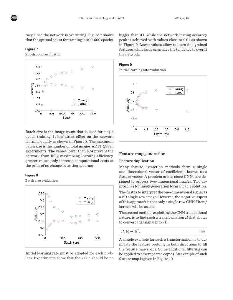
bigger than 0.1, while the network testing accuracy peak is achieved with values close to 0.01 as shown in Figure 9. Lower values allow to learn fine grained features, while large ones have the tendency to overfit the network.

Figure 9 Initial learning rate evaluation

7




��ℝ → ℝ�. (29)



(from left - nearest, bilinear, bicubic filtering) Ac

cura

cy

Feature map generationFeature duplicationMany feature extraction methods form a single one-dimensional vector of coefficients known as a feature vector. A problem arises since CNNs are de-signed to process two-dimensional images. Two ap-proaches for image generation form a viable solution. The first is to interpret the one-dimensional signal as a 2D single row image. However, the negative aspect of this approach is that only a single row CNN filters/kernels will be usable.The second method, exploiting the CNN translational nature, is to find such a transformation H that allows to convert a 1D signal into 2D:

7




��ℝ → ℝ�. (29)




Accu

racy

(29)

A simple example for such a transformation is to du-plicate the feature vector y in both directions to fill the feature map space. Some additional filtering can be applied to new repeated copies. An example of such feature map is given in Figure 10.


Feature map scalingA baseline method and the simplest approach from all feature extraction techniques is to classify the raw EEG signal samples. The raw EEG data form factor of NxM, (where N is number of channels, M is number of samples, N<<M) restricts a direct use of it for CNN feature images due to large number of samples. Thus it must be scaled down. Generally, a feature map of WxH size (where W is width and H is height) can be formed by down/up-scaling the raw EEG signal or extracted feature data. The technique of resizing can use bilinear or other type of filtering in order to prevent sharp data transitions, limit noise and smooth out the final fea-ture map. An example of filtering applied to raw EEG feature maps can be seen in Figure 11.

Figure 10 Feature map generated via vector duplication

7




��ℝ → ℝ�. (29)




Accu

racy

niques are applied. It can be seen that for raw EEG signal analysis nearest filtering method should be used in order to retain original signal details as much as possible. For other feature types the effect could be the opposite.

Figure 11 Example of 22x22 raw EEG feature maps (from left - nearest, bilinear, bicubic filtering)

7




��ℝ → ℝ�. (29)




Accu

racy

Initial testing results of the three different image fil-tering techniques for raw EEG signal classification are given in Table 3. Results show ~10% difference in classification accuracy when various filtering tech-

Table 3 Raw EEG feature map resize filtering accuracy

Filter method Training Testing

Nearest 0.47 ± 0.14 0.43 ± 0.11

Bilinear 0.35 ± 0.11 0.33 ± 0.12

Bicubic 0.33 ± 0.10 0.32 ± 0.11

Feature map and filter dimensionsThe problem is to find the right level of granularity in order to create data abstractions at the proper scale, given a particular dataset. Different feature maps and filter sizes were analyzed for the motor imagery prob-lem. Dimensions from 8x8 to 64x64 of feature maps were tested. Test results are given in Figure 12.

Figure 12 Feature map size evaluation

10 20 30 40 50 60Feature map size

0.4

0.45

0.5

0.55

0.6

0.65

0.7

Accu

racy

TrainingTesting

2 3 4 5 6 7 8 9 10 11Filter size

0.63

0.64

0.65

0.66

0.67

0.68

0.69

0.7 TrainingTesting

The plot shows that the optimal feature map size is 24x24 with accuracy of 65%, even though a more ac-curate solution of 66% exists at size 44x44. Choosing a smaller size feature map ensures faster computation and processing speeds. Also note that the accuracy


convergence is reached when the feature map size is at least twice (15x15) the size as the convolution layer filter size (7x7 in the experiment). When the optimal size is reached, the further increase in dimension only introduces extra computational costs.Convolution layer filter size limits the learning granu-larity by encompassing fixed size feature map regions. Ten different filter sizes were tested in range [2; 11] for 22x22 feature maps. Test results are displayed in Figure 13.

Figure 13 Convolution layer filter size evaluation

The optimal filter size, that gives highest accuracy, is 7x7 and 11x11. Choosing the smaller filter size ensures faster processing speeds. Filters of size 2x2 and 3x3 exhibit too few weights to fully learn the details of the provided data.

ExperimentsThe main purpose of the experimentation activities was to investigate the capabilities of CNN classifier for four-class motor imagery classification problem. Also, to analyze influence of various CNN architec-tures, feature maps, filter sizes and other parameters to classification accuracy. Experiments were con-ducted in the analysis step (tuning the CNN network parameters) and also in the main motor imagery clas-sification step (for each subject).The experiment results were measured and evaluated using normalized accuracy in range [0; 1]. The CNN network parameters were tuned and verified before


0.4

0.45

0.5

0.55

0.6

0.65

0.7

Accu

racy

TrainingTesting

2 3 4 5 6 7 8 9 10 11Filter size

0.63

0.64

0.65

0.66

0.67

0.68

0.69

0.7 TrainingTesting

final classification step. Tests were carried out using ten-fold cross validation. Also, the ability of CNN to learn from feature data was validated visually by in-specting the learned filter/weight images.Final classification results for each subject are pro-vided in the results section further.

DatasetBCI signal Dataset 2a (contributed and described by Brunner et al. [5]) from the BCI IV competition held in 2008 was used for classifier training and testing. The data consists of 22 channels of 250 Hz sample rate re-corded EEG signal for 9 healthy test subjects (total 288 motor imagery trials per subject). The EEG signal was bandpass-filtered between 0.5 Hz and 100 Hz and ad-ditional 50 Hz notch filter was enabled to suppress line noise. For each subject, two sessions on different days were recorded. During each session and using a cue-paced (synchronous) mode of operation, test subjects were asked to imagine movement of one out of four dif-ferent motions (left hand, right hand, feet, tongue) for 3 s. Each of the trials (Figure 14) in the dataset started with an audible signal (beep), followed by visual infor-mation (cue) on screen to perform one of the mental tasks and a short break after the mental task. Before the experiments additional artifact correction of EEG data was done to discard invalid trials as described in [5] by Brunner et al. The corrected EEG data were band-pass-filtered between 7 Hz and 30 Hz in order to cover mu and beta rhythm bands.

Figure 14 Single trial timing scheme


0.4

0.45

0.5

0.55

0.6

0.65

0.7

Accu

racy

TrainingTesting

2 3 4 5 6 7 8 9 10 11Filter size

0.63

0.64

0.65

0.66

0.67

0.68

0.69

0.7 TrainingTesting

Implementation detailsSoftware code for experiments was implemented in MATLAB 2016b/9.1 numerical computation environ-ment. CNN is a new MATLAB functionality (starting from the 2016a/9.0 version), which uses GPU proces-


sor for parallel computations. Other alternatives for convolutional neural networks exist such as the open source MatConvNet library created by Vedaldi and Lenc [17], however, the library was left as an option for future CNN evaluations. Parts of the open source BioSig library for biomedical signal processing and imaging were used in EEG signal analysis. CNN convolution layer initial filter weights in all tests were set to have a Gaussian distribution with a mean of 0 and standard deviation of 0.01. The default for the initial bias was 0.All MATLAB source code used in this work with results are available at the Github Git repository: https://github.com/tomazas/itc2017.

ResultsFinal classification results were obtained after analy-sis and CNN parameter fine-tuning step. A CNN with initial learning rate of 0.01, momentum of 0.1, batch size of 128, 200 epochs and architecture I(22x22)C(4x4,16)RPFSO was trained and tested for final evaluation on all subjects. Results were verified by us-ing 10-fold cross-validation scheme. The accuracies with their standard deviation values are displayed in Table 4. From the results, it can be seen that the best performing approach (70% in training) and (68% in testing) is the FFT energy map method. The second and third best methods in tests are the Channel vari-ance (68%/61%) and Signal energy map (67%/61%) features. The lowest accuracy of (41%/31%) was achieved by the TDP feature method.

ConclusionsThis work analyzed Convolutional Neural Networks and their application to four-class motor-imag-ery based problem. After an in-depth CNN analysis and parameter fine-tuning, promising results were

Table 4 Classification results for feature methods

Method Training Testing

MCE 0.66 ± 0.19 0.58 ± 0.20

CV 0.68 ± 0.18 0.61 ± 0.22

MWP 0.66 ± 0.19 0.58 ± 0.20

PCA 0.61 ± 0.16 0.55 ± 0.20

BP 0.52 ± 0.18 0.39 ± 0.11

CFFT 0.66 ± 0.19 0.58 ± 0.20

DCT 0.54 ± 0.17 0.42 ± 0.11

TDP 0.41 ± 0.11 0.31 ± 0.07

TKEO 0.43 ± 0.12 0.34 ± 0.05

FFTEM 0.70 ± 0.18 0.68 ± 0.20

CWT 0.46 ± 0.10 0.43 ± 0.13

RAW 0.48 ± 0.14 0.37 ± 0.11

SEM 0.67 ± 0.18 0.61 ± 0.20

achieved for the selected problem. The FFT energy map method demonstrated the best feature deter-mination abilities and achieved 68% mean testing accuracy for all the BCI IV competition 2a dataset subjects. The gained accuracy is slightly better than in new techniques proposed by Tabar and Halici in [15] and similar to more complex state-of-the-art EEG analysis techniques by Yang et. al. [21]. The use of simpler feature extraction methods like FFT ener-gy map shows a high CNN method potential for motor imagery EEG analysis.Further work will continue in order to provide more efficient feature extraction methods favoring pro-cessing speed and accuracy.

AcknowledgmentsWe would like to present our thanks to anonymous re-viewers for their helpful suggestions.

References1. Bai, X. Wang, X., Zheng, S., Yu, M. The offline fea-

ture extraction of four-class motor imagery EEG based on ICA and Wavelet-CSP. Control Conference (CCC), 2014, 7189-7194. https://doi.org/10.1109/ChiCC.2014.6896188

2. Bevilacqua, V. et al. A novel BCI-SSVEP based approach for control of walking in Virtual Environment using a Convolutional Neural Network. International Joint Conference on Neural Networks (IJCNN), 2014, 4121-4128. https://doi.org/10.1109/IJCNN.2014.6889955


3. Birvinskas, D., Jusas, V., Martišius, I., Damaševičius, R. EEG dataset reduction and feature extraction using discrete cosine transform. UKSim-AMSS EMS 2012: 6th European Modelling Symposium on Mathemati-cal Modeling and Computer Simulation 2012, 186-191. https://doi.org/10.1109/EMS.2012.88

4. Box, G. E. P., Cox, D. R. An analysis of transformations. Journal of the Royal Statistical Society, Series B, 1964, 26(2), 211-252. http://www.jstor.org/stable/2984418

5. Brunner, C. et al. BCI Competition 2008 – Graz data set A, 2008. http://www.bbci.de/competition/iv/desc_2a.pdf

6. Cecotti, H., Gräser, A. Convolutional neural network with embedded fourier transform for EEG classifica-tion. Proceedings of the 19th International Conference on PatternRecognition (ICPR’08), 2008, 1-4, https://doi.org/10.1109/ICPR.2008.4761638

7. Cecotti, H., Gräser, A. Convolutional neural networks for P300 detection with application to brain–computer interfaces. IEEE Transactions on Pattern Analysis and Machine Intelligence, 2011, 33(3), 433-445, https://doi.org/10.1109/TPAMI.2010.125

8. Hu, J., Mu, Z., Xiao, D. Application of Energy Entropy in Motor Imagery EEG Classification. JDCTA, 2009, 3, 83-90. http://dblp.dagstuhl.de/rec/bib/journals/jdcta/HuXM09

9. LeCun, Y., Bottou, L., Bengio, Y., Haffner, P. Gradi-ent-based learning applied to document recognition. Proceedings of the IEEE, 86(11), 2278-2324. https://doi.org/10.1109/5.726791

10. Le Van Quyen, M., Foucher, J., Lachaux, J., Rodriguez, E., Lutz, A., Martinerie, J., Varela, F. J. Comparison of Hilbert transform and wavelet methods for the analysis of neuronal synchrony. Journal of Neuroscience Meth-ods, 2001, 111, 83-98. https://doi.org/10.1016/S0165-0270(01)00372-7

11. Manor, R., Geva, A. B. Convolutional Neural Network for Multi-Category Rapid Serial Visual Presenta-tion BCI. Frontiers Media S. A, 2015. https://dx.doi.org/10.3389%2Ffncom.2015.00146

12. Mirowski, P., LeCun, Y., Madhavan, D., Kuzniecky, R. Comparing SVM and convolutional networks for epi-leptic seizure prediction from intracranial EEG. IEEE Workshop Machine Learning Signal Processing, 2008. https://doi.org/10.1109/MLSP.2008.4685487

13. Naeem, M., Brunner, C., Pfurtscheller, G. Dimension-ality Reduction and Channel Selection of Motor Im-

agery Electroencephalographic Data. Computational Intelligence and Neuroscience, 2009. http://dx.doi.org/10.1155/2009/537504

14. Qin, L., He, B. A wavelet-based time-frequency anal-ysis approach for classification of motor imagery for brain-computer interface applications. Journal of Neural Engineering, 2005, 2, 65-72. https://doi.org/10.1088/1741-2560/2/4/001

15. Tabar, Y. R., Halici, U. A novel deep learning approach for classification of EEG motor imagery signals. Jour-nal of Neural Engineering, 2016, 14(1), https://doi.org/10.1088/1741-2560/14/1/016003

16. Uktveris, T., Jusas, V. Comparison of Feature Extraction Methods for EEG BCI Classification. Information and Software Technologies: 21st International Conference, 2015, 81-92. https://doi.org/10.1007/978-3-319-24770-0_8

17. Vedaldi, A., Lenc, K. MatConvNet – Convolutional Neu-ral Networks for MATLAB. Proceedings of the ACM International Conference on Multimedia, 2015. https://arxiv.org/abs/1412.4564

18. Wang, D., Miao, D., Blohm, G. Multi-Class Motor Imagery EEG Decoding for Brain-Computer Inter-faces. Frontiers in Neuroscience, 2012. https://doi.org/10.3389/fnins.2012.00151

19. Wang, Y., Gao, S., Gao, X. Common Spatial Pattern Method for Channel Selection in Motor Imagery Based Brain-Computer Interface. IEEE Engineering in Medi-cine and Biology 27th Annual Conference, 2005, 5392-5395. https://doi.org/10.1109/IEMBS.2005.1615701

20. Xiao, D., Mu, Z. D., Hu, J. F. Classification of motor imagery EEG signals based on energy entropy. 2009 International Symposium on Intelligent Ubiquitous Computing and Education, 2009, 61-64. https://doi.org/10.1109/IUCE.2009.57

21. Yang, H., Sakhavi, S., Ang, K. K., Guan, C. On the use of convolutional neural networks and augmented CSP features for multi-class motor imagery of EEG signals classification. 37th Annual International Conference of the IEEE Engineering in Medicine and Biology Soci-ety (EMBC), 2015, 2620-2623, https://doi.org/10.1109/EMBC.2015.7318929

22. Zhou, B. , Wu, X. , Zhang, L. , Lv, Z., Guo, X. Robust Spa-tial Filters on Three-Class Motor Imagery EEG Data Using Independent Component Analysis. Journal of Biosciences and Medicines, 2014, 2, 43-49. http://dx.doi.org/10.4236/jbm.2014.22007


Summary / Santrauka

In this paper the use of a novel feature extraction method oriented to convolutional neural networks (CNN) is discussed in order to solve four-class motor imagery classification problem. Analysis of viable CNN archi-tectures and their influence on the obtained accuracy for the given task is argued. Furthermore, selection of optimal feature map image dimension, filter sizes and other CNN parameters used for network training is in-vestigated. Methods for generating 2D feature maps from 1D feature vectors are presented for commonly used feature types. Initial results show that CNN can achieve high classification accuracy of 68% for the four-class motor imagery problem with less complex feature extraction techniques. It is shown that optimal accuracy highly depends on feature map dimensions, filter sizes, epoch count and other tunable factors, therefore various fine-tuning techniques must be employed. Experiments show that simple FFT energy map generation tech-niques are enough to reach the state of the art classification accuracy for common CNN feature map sizes. This work also confirms that CNNs are able to learn a descriptive set of information needed for optimal electroen-cephalogram (EEG) signal classification.

Straipsnyje analizuojamas naujas bruožų išskyrimo metodas, paremtas sąsukos neuroniniais tinklais (CNN) ir skirtas keturių klasių įsivaizduojamosios motorikos klasifikavimo problemai spręsti. Darbe analizuojamos ga-limos CNN architektūros ir jų įtaka uždavinio tikslumui. Taip pat atliekamas optimalaus bruožų žemėlapio dy-džio pasirinkimo, filtrų dydžio ir kitų CNN tinklui mokyti naudojamų parametrų tyrimas. Pristatomi metodai skirti generuoti 2D bruožų žemėlapius iš 1D bruožų vektorių dažniausiai naudojamiems bruožų tipams. Pirmi-niai rezultatai parodė, jog CNN gali pasiekti 68 % klasifikavimo tikslumą sprendžiant keturių klasių įsivaizduo-jamosios motorikos problemą, net kai taikomi mažiau sudėtingi bruožų išskyrimo metodai. Parodoma, kad op-timalus klasifikavimo tikslumas labai priklauso nuo bruožų žemėlapio dydžio, filtro dydžio, mokymo iteracijų skaičiaus ir kitų faktorių, todėl turi būti taikomos įvairios derinimo metodikos. Atlikus eksperimentus matyti, kad nesudėtingas FFT energijos žemėlapio generavimo metodas yra pakankamas norint pasiekti moderniausių metodų klasifikavimo tikslumą su dažniausiai naudojamais CNN bruožų žemėlapių dydžiais. Straipsnyje taip pat akcentuojama, kad CNN gali išmokti aibę apibūdinančios informacijos, reikalingos elektroencefalogramos (EEG) signalui optimaliai klasifikuoti.

application of convolutional neural networks to four-class

Documents