Int. J. Appl. Math. Comput. Sci., 2015, Vol. 25, No. 4, 927–941DOI: 10.1515/amcs-2015-0066

APPLICATION OF CUBIC BOX SPLINE WAVELETS IN THE ANALYSIS OFSIGNAL SINGULARITIES

WALDEMAR RAKOWSKI a

aFaculty of ManagementBiałystok University of Technology, ul. Stefana Tarasiuka 2, 16-001 Kleosin, Poland

e-mail: w.rakowski@pb.edu.pl

In the subject literature, wavelets such as the Mexican hat (the second derivative of a Gaussian) or the quadratic box splineare commonly used for the task of singularity detection. The disadvantage of the Mexican hat, however, is its unlimitedsupport; the disadvantage of the quadratic box spline is a phase shift introduced by the wavelet, making it difficult to locatesingular points. The paper deals with the construction and properties of wavelets in the form of cubic box splines whichhave compact and short support and which do not introduce a phase shift. The digital filters associated with cubic boxwavelets that are applied in implementing the discrete dyadic wavelet transform are defined. The filters and the algorithmea trous of the discrete dyadic wavelet transform are used in detecting signal singularities and in calculating the measuresof signal singularities in the form of a Lipschitz exponent. The article presents examples illustrating the use of cubic boxspline wavelets in the analysis of signal singularities.

Keywords: cubic box splines, wavelets, dyadic wavelet transform, singularity detection.

1. Introduction

An important issue in signal processing is to determinea representation of the signal, which simplifies furtherextraction of information contained in that signal.Often, the relevant characteristics of the signal arisefrom the existence of points where the signal variesrapidly in value. The derivative of the signal maybe useful in determining the location of these points.However, numerical differentiation of a discrete-timesignal, especially a noisy one, is an ill-conditionedproblem. The initial smoothing of the signal bycalculating the integral,

∫ +∞

−∞f(u) θ(u − t) du = f � θ(t), (1)

may be helpful in solving the problem where f(t) is thesignal processed, θ(t) is the smoothing function with ashort support in relation to the domain of the signal orrapidly vanishing as a Gaussian function, and where

∫ +∞

−∞θ(t) dt �= 0,

θ(t) = θ(−t),

f � θ(t) =

∫ +∞

−∞f(u) θ(t− u) du.

The derivative of the smoothed signal is equal toa convolution of the signal with the derivative of thesmoothing function (see Section 2),

d

dt

[f � θ(t)

]= f � θ

′(t), (2)

where θ′(t) = dθ(t)/dt. It may be useful to smooth

the signal using the scaled smoothing function and todifferentiate the smoothed signal in different scales,

d

dt

∫ +∞

−∞f(u)

1√sθ

(u− t

s

)du =

d

dt

[f � θs(t)

],

(3)where s > 0 is the scale factor. Initial signal smoothingand differentiation of the smoothed signal are particularlyuseful in locating places where the signal has a sharptransition. Such places are called singular points, andtheir determination is referred to as signal singularitydetection (formal definition in Section 6), which applies toone-dimensional signals as well as two-dimensional ones(images).

928 W. Rakowski

As far as the images are concerned, edges are agood illustration of singular places. Smoothing introducesinflection points in the signal where the first derivativehas local extremes and the second one has zero-crossings.Babaud et al. (1986) show that the roots of the secondderivative of the smoothed signal, i.e., the points (t, s) inthe half-plane 0ts (t ∈ R, s > 0) that satisfy the equation

d2

dt2[f � θs(t)

]= 0, (4)

when the smoothing function θ(t) is a Gaussian function,form outlines that end at the singular points of the signalas the scale decreases to zero, s → 0. Points on a coarsescale that satisfy Eqn. (4) allow us to identify (suggestthe existence of) singular positions, while points on afine scale can localize, i.e., determine, the value of thevariable t where the singularity occurs. The ability toidentify singularities in a coarse scale is important becausethe noise present in the signal may suggest the existenceof additional points corresponding to the contours thatappear in fine scales. At coarse scales, the noise is filteredand the appearing contours correspond to real singularpoints of the signal. However, at a coarse scale, due tostrong signal smoothing, it may be difficult to identify thepoints of local extremes, particularly in the discrete form,as the smoothed signal may have the same value at severalneighboring points. In such a case, identifying the pointsforming the contours ending in singular points is allowedby extremes in fine scales.

Smoothing and differentiation of the smoothed signalare directly related to the calculation of the wavelettransform of a signal using the wavelet equal to thederivative of the smoothing function. The mathematicalfoundation of singularity detection using the wavelettransform was presented in several papers. Namely,Mallat (1991) shows the application of the wavelet calledthe Mexican hat (the second derivative of a Gaussian) forsingularity detection. Mallat and Hwang (1992) use aquadratic box spline wavelet. Mallat and Zhong (1992)define filter coefficients corresponding to the quadraticbox spline wavelet.

In this paper, we present the design and applicationof digital filters corresponding to the scaling functionand the wavelet as a cubic box spline to detect signalsingularities. Box splines have a compact and shortsupport; the corresponding filters have finite and shortimpulse responses. The cubic box spline is an evenfunction, and as a consequence there is no phase shiftintroduced by the filter corresponding to that wavelet.

1.1. Definitions. Z denotes the set of integers,L2(R) means the space of measurable, square-integrableone-dimensional functions; l2(Z) means the space ofsquare-summable sequences, also known as the space offinite energy sequences.

The convolution of two continuous-time signalsf(t) ∈ L2(R) and g(t) ∈ L2(R) has the following symboland definition:

f � g(t) =

∫ +∞

−∞f(u) g(t− u) du. (5)

The convolution of two discrete-time signals f [n] ∈ l2(Z)and g[n] ∈ l2(Z) has the following symbol and definition:

f � g[n] =+∞∑

k=−∞f [k] g[n− k]. (6)

The reversed signal in relation to the continuous-timesignal f(t) is

f(t) = f(−t). (7)

The reversed signal in relation to the discrete-time signalf [n] is

f [n] = f [−n]. (8)

The Fourier transform of a continuous-time signal f(t) isdefined as

F (jω) =

∫ +∞

−∞f(t) e−jωt dt. (9)

The Fourier transform of a discrete-time signal f [n] isdefined as

F (ejω) =

+∞∑n=−∞

f [n] e−jωn. (10)

The scaled function fs(t) is defined as

fs(t) =1√sf

(t

s

). (11)

The scaled and translated function fu,s(t) is defined as

fu,s(t) =1√sf

(t− u

s

). (12)

θ′(t) represents the first derivative of the function θ(t),thus θ′(t) = dθ(t)/dt; θ′′(t) represents the secondderivative of the function θ(t), thus θ′′(t) = d2θ(t)/dt2.

2. Wavelet analysis

In a wavelet analysis, there are two functions: a scalingfunction φ(t) and a wavelet ψ(t), and two digital filters:a low-pass filter h and a high-pass filter g. In termsof signal processing, the scaling function is an impulseresponse of a low-pass filter and the wavelet is an impulseresponse of a band-pass filter. Both the wavelet and thescaling function are characterized by fast decay, e.g., anexponential or compact support. Relations between the

Application of cubic box spline wavelets in the analysis of signal singularities 929

scaling function, the wavelet and the filters are describedby the following two equations:

1√2φ(t/2) =

∑n

h[n] φ(t − n), (13)

1√2ψ(t/2) =

∑n

g[n] φ(t− n). (14)

Equation (13) is called the dilation equation. Acharacteristic feature of the scaling function is a non-zerovalue of the following integral:

∫ +∞

−∞φ(t) dt �= 0. (15)

It is assumed that ||φ(t)|| = 1. The coefficient 1/√2

ensures preservation of the norm of the scaled functionin the space L2(R). In the frequency domain, the scalingequation takes the form of

Φ(j2ω) =1√2H(ejω) Φ(jω). (16)

The Fourier transform of the scaling function as a transferfunction of a low-pass filter is not equal to zero for ω = 0,i.e., Φ(j0) �= 0. It is assumed that H(ej0) =

√2, which

means that∑+∞

n=−∞ h[n] =√2. The dilation equation

allows calculating the low-pass filter h for a given scalingfunction φ(t).

Equation (14) is called the wavelet equation. Themain feature of the wavelet is a vanishing integral of thewavelet, i.e., ∫ +∞

−∞ψ(t) dt = 0. (17)

In the frequency domain, the wavelet equation takes theform

Ψ(j2ω) =1√2G(ejω) Φ(jω). (18)

Since Φ(j0) �= 0, the number of zeros p of the transferfunction G(jω) for ω = 0 determines the number ofzeros of the Fourier transform of Ψ(jω) for ω = 0. Itis equivalent to the fact that the wavelet has p vanishingmoments, thus

∫ +∞

−∞tkf(t) dt = 0, 0 ≤ k ≤ p− 1. (19)

This property indicates that the wavelet is orthogonal tothe polynomial of degree k ≤ p−1. The wavelet equationallows calculating the wavelet for a given scaling functionφ(t) and a given high-pass filter g.

A wavelet transform of a continuous-time signal (acontinuous spatial variable) is a function of two variablesand is a measure of the similarity between the signalf(t) and the wavelet ψu,s(t) at scale s, shifted to the

time instant t = u. The formal definition of a wavelettransform of a continuous-time signal is

Wf(u, s) =

∫ +∞

−∞f(t)

1√sψ

(t− u

s

)dt

=

∫ +∞

−∞f(t)

1√sψ

(u− t

s

)dt

(20)

and has the following symbolic notation:

Wf(u, s) = f � ψs(u). (21)

The coefficient 1/√s that appears before the scaled and

shifted wavelet preserves the norm of the scaled waveletin the space L2(R).

The relationship between the continuous-timewavelet transform and a derivative of the smoothed signalis shown by the following calculations:

d

dt

[f � θs(t)

]=

d

dt

∫ ∞

−∞f(u)

1√sθ

(t− u

s

)du

=

∫ ∞

−∞f(u)

1√s

[d

dtθ

(t− u

s

)]du

=1

s

∫ ∞

−∞f(u) θ

′s(t− u) du

=1

sf � θ

′s(t). (22)

The last equation means that the derivative of the signalsmoothed by the scaled smoothing function is equal to theconvolution of the signal with a derivative of the scaledsmoothing function (with the accuracy to coefficient 1/s).

We define the wavelet in the form of a derivative ofthe smoothing function with a minus sign,

ψ(t) = −θ′(t), (23)

which is equivalent to

ψ(t) = θ′(t), (24)

ψs(t) = θ′s(t). (25)

Taking into account (22) and (25), we obtain

d

dt

[f � θs(t)

]=

1

sf � ψs(t). (26)

Thus, in accordance with (21),

Wf(t, s) = sd

dt

[f � θs(t)

]. (27)

The wavelet can also take the form of the secondderivative of the smoothing function:

ψ(t) = θ′′(t). (28)

930 W. Rakowski

Then

Wf(t, s) = s2d2

dt2[f � θs(t)

]. (29)

In the case of wavelets which are the first derivativeof the smoothing function, singular points correspond tothe modulus maxima of the wavelet transform; in thecase of wavelets which are the second derivative of thesmoothing function, singular points correspond to thezero-crossing of the wavelet transform.

Examples of wavelets in the form of the first andsecond derivatives of the smoothing function are shownin Section 4.

The wavelet transform is an effective tool forsingularity detection. Mallat (1991), Mallat and Hwang(1992) as well as Mallat and Zhong (1992) show that, ifthe scale factor s tends to zero, then the points (t, s) onthe half-plane t ∈ R, s > 0 corresponding to the modulusmaxima of the wavelet transformWf(t, s) represent linesthat end in the singular points of the signal.

2.1. Dyadic signal representation. The signalrepresentation in the form of a continuous-time wavelettransform which is a function of two variables (time andscale) is a highly redundant representation. It is proven(Mallat, 2009) that the signal can be reconstructed froma dyadic wavelet transform, in which the scale is not acontinuous variable but a countable set of dyadic values:{sk}k∈Z, where sk = 2k.

The dyadic wavelet transform is defined as follows:

W2kf(u) =

∫ +∞

−∞f(t)

1√2k

ψ

(t− u

2k

)dt

= f � ψ2k(u),

(30)

where k ∈ Z. This transform is a countable set offunctions of one variable (time or space).

In the frequency domain, the dyadic wavelettransform is expressed as

W2kF (jω) =√2k F (jω) Ψ(j2kω). (31)

To calculate the wavelet transform at points (n, 2k),n, k ∈ Z (linearly spaced points in time and a dyadicscale), a fast algorithm can be used which is called inFrench algorithme a trous (Holschneider et al., 1989;Shensa, 1992).

The first step is to define a rectangle [tmin, tmax] ×[smin, smax] in which the values of the wavelet transformwill be calculated. Two rectangles are commonly used:[0, N−1]×[2, smax] or [0, 1)×[smin, 1], whereN = 2K .In the case of the rectangle [0, N − 1] × [2, smax],the wavelet transform values W2kf(n) are calculated inpoints n = 0, 1, . . . , N − 1, for k = 1, 2, . . . ,K , whereK = log2N . In the case of the rectangle [0, 1) ×[smin, 1], the wavelet transform values W2kf(n/N) are

calculated at points n = 0, 1, . . . , N − 1, for k = −(K −1),−(K − 2), . . . , 0.

The application of the a trous algorithm to computethe wavelet transform requires the knowledge the digitalrepresentation of the signal f(t) in the finest scale, i.e.,scale s = 1 in the case of window [0, N − 1]× [2, smax]or scale s = 1/N in the case of window [0, 1)× [smin, 1].From now, on the descriptions of the algorithms willconcern the rectangle [0, N − 1]× [2, smax] on the plane0ts.

2.2. Discrete dyadic wavelet transform. Let

dk[n] =W2kf(n), (32)

aK [n] =

∫ +∞

−∞f(u)

1√2K

φ

(u− n

2K

)du

= f � φ2K (n),

(33)

k = 1, 2, . . . ,K and n = 0, 1, . . . , N − 1.The sequence of the numbers

{ { dk[n] } n=0,1,...,N−1 } k=1,2,...,K , (34)

{ aK [n] } n=0,1,...,N−1 (35)

is called the discrete dyadic K-level wavelet transform ofsignal f(t).

The wavelet coefficient dk[n] is a measure of thesimilarity (in the sense of the inner product) of signal f(t)in the surrounding of time instant (a point in space) t = nto the wavelet ψ

(t/2k

)or the value of the signal filtered

with a band-pass filter with the impulse responseψ(t/2k

)at t = n.

The coefficient aK [n] is a measure of a similarity ofsignal f(t) in the surrounding of the time instant t = n tothe scaling function φ

(t/2K

)or the value of the signal

filtered by a low-pass filter with the impulse responseφ(t/2K

)at t = n.

A fast algorithm for computing a discrete dyadicwavelet transform by using digital filtering is describedin Section 2.4.

The following section describes how to obtaina discrete-time signal {a0[n]}n∈Z which is a digitalrepresentation of the signal f(t) at the finest scale andforms input to the a trous algorithm for the calculationof a discrete dyadic wavelet transform.

2.3. Digital representation of the signal at the finestscale. The sequence of numbers equal to the innerproduct of signal f(t) and the translation of the scalingfunction φ(t− n)

a0[n] =

∫ +∞

−∞f(t) φ(t− n) dt, n ∈ Z (36)

Application of cubic box spline wavelets in the analysis of signal singularities 931

is a discrete representation of signal f(t) at scale 20. Byintroducing in the above equation a new variable u = t−n, we obtain

a0[n] =

∫ +∞

−∞f(n+ u) φ(u) du, n ∈ Z, (37)

showing that the n-th sample of the discrete signal isproduced by the averaging signal f(t) in the surroundingof the time instant t = n, with the scaling function φ(u)as a weighing function. The sequence (a0[n]) can also beconsidered a sample of the signal filtered by the filter withthe impulse response equal φ(t) = φ(−t). Indeed, let thesignal f0(t) be the result of filtration. Thus,

f0(t) =

∫ +∞

−∞f(u) φ(t− u) du, (38)

and then a0[n] = f0(n). The Fourier transform of signalf0(t) is given by

F0(jω) = F (jω) Φ(jω). (39)

2.4. Algorithme a trous. In order to describe thealgorithm for computing the discrete dyadic wavelettransform, numerical sequences are introduced anddefined as follows:

ak[n] =

∫ +∞

−∞f(u)

1√2k

φ

(u− n

2k

)du

= f � φ2k(n),

(40)

dk[n] =

∫ +∞

−∞f(u)

1√2k

ψ

(u− n

2k

)du

= f � ψ2k(n),

(41)

n = 0, 1, . . . , N − 1 and k = 1, . . . ,K .Let hk = (hk[n]), k ≥ 0, be a digital filter with

the impulse response created from the impulse responseof filter h = (h[n]) in such a way that, between each twoadjacent coefficients of filter h, 2k − 1 zeros are inserted,and hk[n] = hk[−n]; analogically, this is applied tofilters gk. The coefficients of the discrete dyadic wavelettransform of signal a0 can be calculated in the iterativeprocess specified in the following theorem.

Theorem 1. For k ≥ 0,

dk+1[n] = ak � gk[n], (42)

ak+1[n] = ak � hk[n]. (43)

Proof. The proof of this theorem can be found in the bookof Mallat (2009). �

gk dk+1

hk ak+1

ak

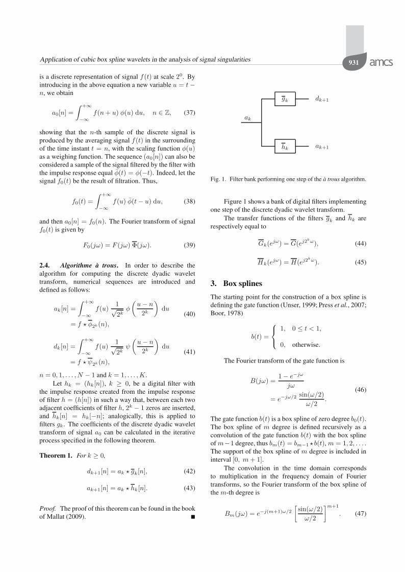
Fig. 1. Filter bank performing one step of the a trous algorithm.

Figure 1 shows a bank of digital filters implementingone step of the discrete dyadic wavelet transform.

The transfer functions of the filters gk and hk arerespectively equal to

Gk(ejω) = G(ej2

kω), (44)

Hk(ejω) = H(ej2

kω). (45)

3. Box splines

The starting point for the construction of a box spline isdefining the gate function (Unser, 1999; Press et al., 2007;Boor, 1978)

b(t) =

⎧⎨⎩

1, 0 ≤ t < 1,

0, otherwise.

The Fourier transform of the gate function is

B(jω) =1− e−jω

jω

= e−jω/2 sin(ω/2)

ω/2.

(46)

The gate function b(t) is a box spline of zero degree b0(t).The box spline of m degree is defined recursively as aconvolution of the gate function b(t) with the box splineofm−1 degree, thus bm(t) = bm−1 �b(t), m = 1, 2, . . . .The support of the box spline of m degree is included ininterval [0, m+ 1].

The convolution in the time domain correspondsto multiplication in the frequency domain of Fouriertransforms, so the Fourier transform of the box spline ofthe m-th degree is

Bm(jω) = e−j(m+1)ω/2

[sin(ω/2)

ω/2

]m+1

. (47)

932 W. Rakowski

The box spline of degreem can be calculated by using thebox splines of degreem− 1,

bm(t) = [ t bm−1(t) + (m+ 1− t) bm−1(t− 1) ] /m.(48)

The derivative of box spline of degreem can be calculatedby using the box spline of degree m− 1,

b′m(t) = bm−1(t)− bm−1(t− 1). (49)

The integer translations of box splines bm(t− n), n ∈ Z,are not orthogonal to one another. Thus

∫ +∞

−∞bm(t− n) bm(t− k) dt �= δ[n− k]. (50)

There is a procedure of orthogonalization; however,splines received as a result do not have a compact supportbut decay quickly (exponentially).

3.1. Box spline of the third degree. The box spline ofdegree 3 b3(t) has a support equal to interval [0, 4].

On each of the subintervals [k, k + 1], 0 ≤ k ≤3, the value of the function is determined by anotherpolynomial of the third degree, but a connection ofdifferent polynomials in the internal nodes, i.e., at pointst = 1, 2, 3, is twice continuously differentiable.

Table 1 shows polynomials defining the box splineof the third degree, and Fig. 2 presents the shape of thefunction.

Table 1. Polynomials describing the box spline of the third de-gree b3(t).

Interval b3(t)

t < 0 0

0 ≤ t < 1 16t3

1 ≤ t < 2 − 12t3 + 2t2 − 2t+ 2

3

2 ≤ t < 3 − 12(4− t)3 + 2(4− t)2 − 2(4− t) + 2

3

3 ≤ t < 4 16(4− t)3

t ≥ 4 0

The Fourier transform of the cubic box spline is

B3(jω) = e−j2ω

[sin(ω/2)

ω/2

]4. (51)

4. Scaling function and wavelet in the formof a cubic box spline

The scaling function is expressed as a box spline functionof the third degree shifted to the left by two units. Thus

φ(t) = b3(t+ 2). (52)

-0.5 0 0.5 1 1.5 2 2.5 3 3.5 4 4.50

0.1

0.2

0.3

0.4

0.5

0.6

0.7

Fig. 2. Box spline of the third degree b3(t).

Figure 3 shows the graph of the scaling function andTable 2 the polynomials describing that function.

The Fourier transform of the scaling function is equal

-2.5 -2 -1.5 -1 -0.5 0 0.5 1 1.5 2 2.50

0.1

0.2

0.3

0.4

0.5

0.6

0.7

Fig. 3. Scaling function φ(t) in the form of translation of thecubic box spline.

Table 2. Polynomials describing the scaling function φ(t) in theform of the cubic box spline.

Interval φ(t)

t < −2 0

−2 ≤ t < −1 (t+ 2)3/6

−1 ≤ t < 0 −t3/2− t2 + 2/3

0 ≤ t < 1 t3/2− t2 + 2/3

1 ≤ t < 2 (2− t)3/6

t ≥ 2 0

Application of cubic box spline wavelets in the analysis of signal singularities 933

-10 -8 -6 -4 -2 0 2 4 6 8 100

0.2

0.4

0.6

0.8

1

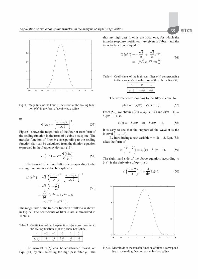
Fig. 4. Magnitude of the Fourier transform of the scaling func-tion φ(t) in the form of a cubic box spline.

to

Φ(jω) =

[sin(ω/2)

ω/2

]4. (53)

Figure 4 shows the magnitude of the Fourier transform ofthe scaling function in the form of a cubic box spline. Thetransfer function of filter h corresponding to the scalingfunction φ(t) can be calculated from the dilation equationexpressed in the frequency domain (13),

H(ejω

)=

√2Φ(j2ω)

Φ(jω). (54)

The transfer function of filter h corresponding to thescaling function as a cubic box spline is

H(ejω

)=

√2

(sinω

ω

)4 [sin(ω/2)

ω/2

]−4

=√2(cos

ω

2

)4

=

√2

16

(ej2ω + 4 ejω + 6

+4 e−jω + e−j2ω).

(55)

The magnitude of the transfer function of filter h is shownin Fig. 5. The coefficients of filter h are summarized inTable 3.

Table 3. Coefficients of the lowpass filter h[n] corresponding tothe scaling function φ(t) as a cubic box spline.

n −2 −1 0 1 2

h[n]√

216

√2

43√

28

√2

4

√2

16

The wavelet ψ(t) can be constructed based onEqn. (14) by first selecting the high-pass filter g. The

shortest high-pass filter is the Haar one, for which theimpulse response coefficients are given in Table 4 and thetransfer function is equal to

G(ejω

)= −

√2

2+

√2

2e−jω

= −j√2 e−j ω2 sin

ω

2.

(56)

Table 4. Coefficients of the high-pass filter g[n] correspondingto the wavelet ψ(t) in the form of the cubic spline (57).

n 0 1

g[n] −√

22

√2

2

The wavelet corresponding to this filter is equal to

ψ(t) = −φ(2t) + φ(2t− 1). (57)

From (52), we obtain φ(2t) = b3(2t+2) and φ(2t− 1) =b3(2t+ 1), so

ψ(t) = −b3(2t+ 2) + b3(2t+ 1). (58)

It is easy to see that the support of the wavelet is theinterval [−1, 1.5].

By introducing a new variable τ = 2t+ 2, Eqn. (58)takes the form of

− ψ

(τ − 2

2

)= b3(τ)− b3(τ − 1). (59)

The right hand-side of the above equation, according to(49), is the derivative of b4(τ), so

ψ

(τ − 2

2

)= − d

dτb4(τ). (60)

-4 -3 -2 -1 0 1 2 3 40

0.5

1

1.5

Fig. 5. Magnitude of the transfer function of filter h correspond-ing to the scaling function as a cubic box spline.

934 W. Rakowski

Going back to the variable t, we obtain

ψ(t) = − d

dt

[1

2b4(2t+ 2)

], (61)

which means that the smoothing function is equal to

θ(t) =1

2b4(2t+ 2) (62)

and ψ(t) = −θ′(t).The Fourier transform of the wavelet is calculated

using the wavelet equation (14),

Ψ(jω) =1√2G(ej

ω2 ) Φ(jω/2)

=−jω4

e−j ω4

[sin(ω/4)

ω/4

]5.

(63)

The transfer function of filter g expressed by theformula (56) has one zero for ω = 0, so the correspondingwavelet has one vanishing moment.

Table 5. Polynomials describing the wavelet ψ(t) in the form ofa cubic spline corresponding to filter g with coefficientsgiven in Table 4.

Interval ψ(t)

t < −1 0

−1 ≤ t < −0.5 − 43(1 + t)3

−0.5 ≤ t < 0 163t3 + 6t2 + t− 1

2

0 ≤ t < 0.5 −8t3 + 6t2 + t− 12

0.5 ≤ t < 1 163t3 − 14t2 + 11t − 13

6

1 ≤ t < 1.5 43( 32− t)3

t ≥ 1.5 0

Table 6. Smoothing function θ(t) in the form of a scaled andtranslated box spline of the fourth degree.

Interval θ(t)

t < −1 0

−1 ≤ t < −0.5 − 13(1 + t)4

−0.5 ≤ t < 0 − 43t4 − 2t3 − 1

2t2 + 1

2t+ 11

48

0 ≤ t < 0.5 2t4 − 2t3 − 12t2 + 1

2t+ 11

48

0.5 ≤ t < 1 − 43t4 + 14

3t3 − 11

2t2 + 13

6t+ 1

48

1 ≤ t < 1.5 13(1.5− t)4

t ≥ 1.5 0

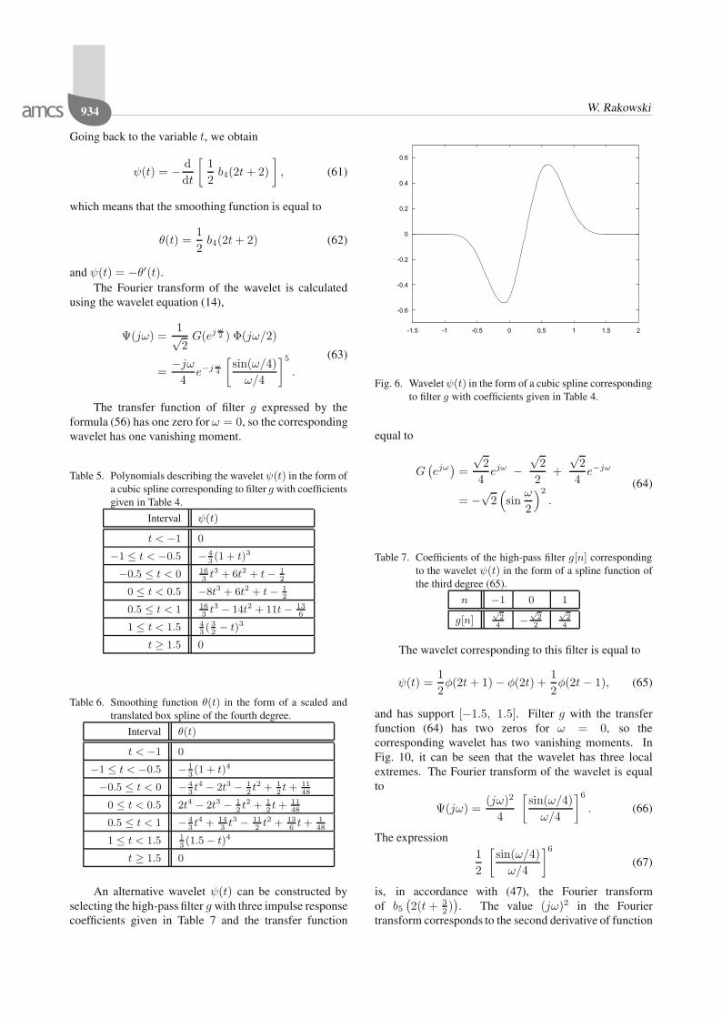
An alternative wavelet ψ(t) can be constructed byselecting the high-pass filter g with three impulse responsecoefficients given in Table 7 and the transfer function

-1.5 -1 -0.5 0 0.5 1 1.5 2

-0.6

-0.4

-0.2

0

0.2

0.4

0.6

Fig. 6. Wavelet ψ(t) in the form of a cubic spline correspondingto filter g with coefficients given in Table 4.

equal to

G(ejω

)=

√2

4ejω −

√2

2+

√2

4e−jω

= −√2(sin

ω

2

)2

.

(64)

Table 7. Coefficients of the high-pass filter g[n] correspondingto the wavelet ψ(t) in the form of a spline function ofthe third degree (65).

n −1 0 1

g[n]√2

4−

√2

2

√2

4

The wavelet corresponding to this filter is equal to

ψ(t) =1

2φ(2t+ 1)− φ(2t) +

1

2φ(2t− 1), (65)

and has support [−1.5, 1.5]. Filter g with the transferfunction (64) has two zeros for ω = 0, so thecorresponding wavelet has two vanishing moments. InFig. 10, it can be seen that the wavelet has three localextremes. The Fourier transform of the wavelet is equalto

Ψ(jω) =(jω)2

4

[sin(ω/4)

ω/4

]6. (66)

The expression1

2

[sin(ω/4)

ω/4

]6(67)

is, in accordance with (47), the Fourier transformof b5

(2(t+ 3

2 )). The value (jω)2 in the Fourier

transform corresponds to the second derivative of function

Application of cubic box spline wavelets in the analysis of signal singularities 935

-15 -10 -5 0 5 10 150

0.05

0.1

0.15

0.2

0.25

0.3

0.35

0.4

0.45

0.5

Fig. 7. Magnitude of the Fourier transform of the wavelet ψ(t)in the form of a cubic spline corresponding to filter gwith coefficients given in Table 4.

b5(2(t+ 3

2 )). Thus, the wavelet

ψ(t) =d2

dt2

{1

2b5

[2

(t+

3

2

)]}, (68)

and the smoothing function is

θ(t) =1

2b5(2t+ 3). (69)

The discussed wavelet is similar to the Mexican hatwavelet, described by

ψ(t) =2

π1/4√3(t2 − 1)e−t2/2 (70)

and shown in Fig. 12.The Mexican hat wavelet is the second derivative

of the Gaussian function. The Gaussian function isthe result of convolution of an infinite number of gatefunctions, i.e., limm→+∞ bm(t); it belongs to the spaceof function C∞ and, as the scale factor tends to zero, theGaussian function tends to the Dirac distribution δ(t). Thewhole axis (−∞, + ∞) is the support of the Gaussianfunction and the Mexican hat wavelet. The Mexicanhat wavelet was the first one used for multiscale filtering(Witkin, 1983; 1984) and detection of signal singularities(Mallat, 1991).

If there is a need for having synthesis filters(reconstruction filters), then a low-pass filter of thesynthesis can be assumed equal to the low-pass filteranalysis, i.e., h = h, as a consequence of the synthesisscaling function φ(t) = φ(t). The transfer function of thehigh-pass synthesis filter g can be calculated from the con-ditions of a perfect signal reconstruction (Mallat, 2009;

-1.5 -1 -0.5 0 0.5 1 1.5 20

0.05

0.1

0.15

0.2

0.25

0.3

0.35

Fig. 8. Smoothing function θ(t) in the form of a scaled andtranslated box spline of the fourth degree.

-20 -15 -10 -5 0 5 10 15 200

0.2

0.4

0.6

0.8

1

Fig. 9. Magnitude of the Fourier transform of the smoothingfunction θ(t) as a scaled and translated box spline of thefourth degree.

Rakowski, 2003) expressed by

H(ejω) H∗(ejω) + G(ejω) G∗(ejω) = 2, (71)

from which

G(ejω) =2− |H(ejω)|2G∗(ejω)

. (72)

Having the transfer function of the filter G(ejω), one cancalculate the coefficients of the impulse response g[n],and the synthesis wavelet ψ(t) is calculated using thewavelet equation (14). Different synthesis wavelet filterscalculated with the FFT algorithm are presented by Zhaoet al. (2013).

936 W. Rakowski

-2 -1.5 -1 -0.5 0 0.5 1 1.5 2

-0.5

-0.4

-0.3

-0.2

-0.1

0

0.1

0.2

0.3

Fig. 10. Wavelet ψ(t) in the form of a cubic spline correspond-ing to filter g with coefficients given in Table 7.

5. Scale-frequency analysis of a dyadicwavelet transform

Multiscale signal decomposition by a dyadic wavelettransform can be seen as a band decomposition of a signalin the frequency domain.

Figure 13 shows a filter configuration carryingK-level discrete dyadic decomposition of signal a0. Itfollows from it that the Fourier transform of signals dk,k = 1, 2, . . . ,K , can be expressed as

D1(ejω) = A0(e

jω) G0(ejω), (73)

Dk(ejω) = A0(e

jω) Gk−1(ejω)

k−2∏l=0

H l(ejω), (74)

k = 2, 3, . . . ,K. Defining the equivalent filter transferfunctions at scales 2k, k = 1, 2, . . . ,K , as

Pk(ejω) = Dk(e

jω)/A0(ejω) (75)

and taking into account (44) and (45), we obtain

P1(ejω) = G(ejω), (76)

Pk(ejω) = G(ej2

k−1ω)

k−2∏l=0

H(ej2lω), (77)

k = 2, 3, . . . ,K.In the case of filters h, g with real impulse response

coefficients, the transfer functions take the form of

P1(ejω) = G∗(ejω), (78)

Pk(ejω) = G∗(ej2

k−1ω)

k−2∏l=0

H∗(ej2lω), (79)

k = 2, 3, . . . ,K .

-25 -20 -15 -10 -5 0 5 10 15 20 250

0.5

1

1.5

Fig. 11. Magnitude of the Fourier transform of the wavelet ψ(t)in the form of a cubic spline corresponding to filter gwith coefficients given in Table 7.

5.1. Frequency characteristics of the equivalent cu-bic filters. The starting point for the construction of thefrequency characteristics of the equivalent cubic filtersPk , k = 2, 3, . . . ,K , is a transfer function of the filterassociated with the scaling function (55),

H(ejω) =√2(cos

ω

2

)4

, (80)

and a transfer function of the filter associated with awavelet.

5.1.1. Wavelet as the first derivative of a smoothingfunction. In this case, the smoothing function is a boxspline of the fourth degree and the wavelet is a cubic boxspline. A transfer function of the filter corresponding tothe wavelet as the first derivative of a smoothing function,according to (56), is equal to

G(ejω) = −j√2 e−j ω

2 sinω

2. (81)

Transfer functions of equivalent filters are obtained afterinserting (80) and (81) into (78) and (79). Figure 14 showsthe magnitudes of the filter transfer functions at scales22, 23, 24, 25. Table 8 presents 3dB pass-bands of thesefilters.

5.1.2. Wavelet as the second derivative of a smooth-ing function. In this case, the smoothing function is abox spline of the fifth degree and the wavelet is a cubicspline. A transfer function of the filter associated withthe wavelet in the form of the second derivative of asmoothing function, according to (64), is equal to

G(ejω) = −√2(sin

ω

2

)2

. (82)

Application of cubic box spline wavelets in the analysis of signal singularities 937

-5 -4 -3 -2 -1 0 1 2 3 4 5-1

-0.5

0

0.5

Fig. 12. Mexican hat wavelet.

a0

g0

d1

h0a1

g1

d2

hk−2ak−1

gk−1

dk

Fig. 13. Filter bank implementing the a trous algorithm.

Transfer functions of the equivalent filters areobtained after inserting (80) and (82) into (78) and (79).Figure 15 shows magnitudes of the transfer functions ofthe equivalent filters at scales 22, 23, 24, 25. Table 9 shows3 dB passband of these filters.

6. Regularity and singularity of a signal

The formal definition of the singularity of a signal isassociated with the Lipschitz exponent and Lipschitzregularity, explained below. If the signal f(t) isdifferentiable, then the number of the derivatives is ameasure of its smoothness. Let the signal f(t) have theFourier transform F (jω) and be m-times differentiable.The Fourier transform of the m-th derivative of the signalis (jω)mF (jω). If the value of α is in the intervalm ≤ α < m+ 1 and such that

∫ +∞

−∞|F (jω)| ( 1 + |ω|α) dω < +∞, (83)

a) | P2(ej�) | (prim)

0 0.1 0.2 0.3 0.40

0.5

1

1.5b) | P3(ej�) | (prim)

0 0.1 0.2 0.3 0.40

0.5

1

1.5

c) | P4(ej�) | (prim)

0 0.1 0.2 0.3 0.40

0.5

1

1.5

2d) | P5(ej�) | (prim)

0 0.1 0.2 0.3 0.40

1

2

3

Fig. 14. Magnitudes of the filter transfer functions associatedwith the cubic box wavelet in the form of the firstderivative of the smoothing function at scales 22, 23,24, 25.

Table 8. 3 dB pass bands of equivalent filters Pk(ejω) at scales

s = 2k, k = 1, 2, 3, 4, 5

Scale Passband 3 dB [rad]

s = 21 0.2500 0.5000

s = 22 0.0654 0.2129

s = 23 0.0303 0.0986

s = 24 0.0156 0.0488

s = 25 0.0078 0.0234

then it is said that the signal f(t) is uniformly Lipschitzwith exponent α. If the supremum of values α satisfiesthe above condition of convergence of the integral, thenthe supremum is a measure of the global regularity ofthe signal. The notion of regularity is an extensionof the concept of smoothness measured by the numberof derivatives. For example, the scaling functionscorresponding to the 9/7 low-pass filters (Fig. 16) usedin the JPEG2000 image compression standard (Skodraset al., 2001) have Lipschitz exponents equal respectivelyto 1.07 and 1.70 (Unser and Blu, 2003).

The Fourier transform of the signal does not allowdetermination of the local regularity of the signal, i.e., theregularity at a point and its surrounding. Point regularityin terms of the Lipschitz exponent is associated withestimation of the error of signal approximation by theTaylor polynomial.

Let the signal f(t) have m continuous derivatives.The Taylor polynomial

pv(t) = f(v) +

m∑k=1

f (k)(t)

k!(t− v)k (84)

938 W. Rakowski

a) | P2(ej�| (bis)

0 0.1 0.2 0.3 0.4 0.50

0.5

1b) | P3(ej�| (bis)

0 0.1 0.2 0.3 0.4 0.50

0.5

1

1.5

c) | P4(ej�| (bis)

0 0.1 0.2 0.3 0.4 0.50

0.5

1

1.5d) | P5(ej�| (bis)

0 0.1 0.2 0.3 0.4 0.50

1

2

3

Fig. 15. Magnitudes of the transfer functions of the equivalentfilters associated with the cubic wavelet as the secondderivative of the smoothing function at scales 22, 23,24, 25.

Table 9. 3 dB pass bands of equivalent filters Pk(ejω) at scales

s = 2k, k = 1, 2, 3, 4, 5.

scale 3 dB band [rad]

s = 21 0.3184 0.5000

s = 22 0.1045 0.2344

s = 23 0.0498 0.1104

s = 24 0.0244 0.0547

s = 25 0.0127 0.0264

approximates the signal f(t) in the neighborhood of pointv with the error

ev(t) = f(t)− pv(t). (85)

The Lipschitz exponent estimates the approximation errorand determines the regularity of the signal in the followingway (Mallat, 2009):

• At a point the signal f(t) has v the Lipschitzexponent α ≥ 0 if there exist a constant K > 0 andpolynomial pv(t) of degree m = α such that, foreach t ∈ R,

| f(t)− pv(t) | ≤ K |t− v|α. (86)

• The signal f(t) is uniformly Lipschitz α into interval[a, b] if it satisfies the Lipschitz condition (86) for allv ∈ [a, b] with a constant K independent of v.

• The Lipschitz regularity of the signal f(t) at a point vor in the interval [a, b] is defined by the supremum ofthe values α such that f(t) has Lipschitz exponentα.

a) filter of length 9

-4 -2 0 2 4-0.4

-0.2

0

0.2

0.4

0.6

0.8

1

1.2

1.4b) filter of length 7

-2 0 2-0.4

-0.2

0

0.2

0.4

0.6

0.8

1

1.2

1.4

Fig. 16. Scaling functions corresponding to 9/7 biorthogonal fil-ters.

If 0 ≤ α < 1, then the signal is non-differentiable at thepoint v and the Lipschitz condition is expressed by thefollowing inequality:

| f(t)− f(v) | ≤ K |t− v|α. (87)

A signal that is bounded but non-continuous at apoint v has the Lipschitz exponent equal to 0. If 0 < α <1, then the signal at the point v is singular. If α ≥ 1, thenf (p)(t), where p = α has the Lipschitz exponent equalto α− p, and if α− p > 0, then that value is a measure ofthe singularity of the p-th derivative of the signal f(t).

A wavelet transform of a signal, calculated with awavelet that has enough vanishing moments is equal to thewavelet transform of the error approximation (85). Let thevanishing moment number p of the wavelet be no less thanthe Lipschitz exponent α, i.e., p ≥ α. Thus,

Wf(t, s) =Wpv(t, s) +Wev(t, s)

=Wev(t, s),(88)

because the wavelet is orthogonal to pv(t). It followsthat, if 0 ≤ α ≤ 1, then a wavelet with one vanishingmoment can be used; if 1 < α ≤ 2, then a wavelet withtwo vanishing moments should be used. Among all thesingular points, the so-called isolated singularities standout. A point v is an isolated singular point if the maximumvalues of the wavelet transform modulus at a scale s lessthan a certain scale s0 are located in a cone

|t− v| ≤ Cs, (89)

where C is a certain positive constant. Mallat (2009)shows that in the case of the isolated singular points thereexists a constant A > 0 such that

|Wf(t, s)| ≤ A sα+1/2. (90)

Application of cubic box spline wavelets in the analysis of signal singularities 939

An equivalent form can be obtained by applying alogarithm on both sides of the inequality

log2 |Wf(t, s)| ≤ (α+ 1/2) log2 s+ log2 A, (91)

from which it follows that α+ 1/2 is the maximum slopeof a straight line y = rx + q, where x = log2 s and y =log2 |Wf(t, s)|.

7. Numerical results

Below are two examples illustrating the use of a discretedyadic wavelet transform and cubic wavelets for detectionof slopes (edges) of the signal.

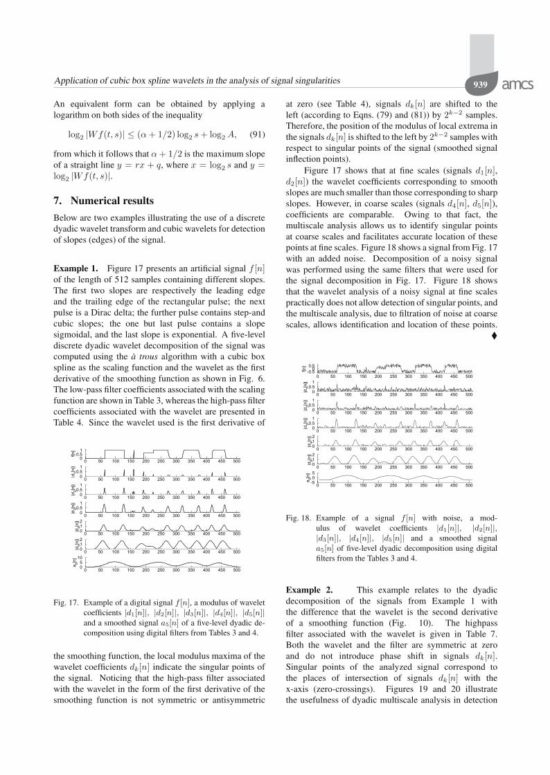
Example 1. Figure 17 presents an artificial signal f [n]of the length of 512 samples containing different slopes.The first two slopes are respectively the leading edgeand the trailing edge of the rectangular pulse; the nextpulse is a Dirac delta; the further pulse contains step-andcubic slopes; the one but last pulse contains a slopesigmoidal, and the last slope is exponential. A five-leveldiscrete dyadic wavelet decomposition of the signal wascomputed using the a trous algorithm with a cubic boxspline as the scaling function and the wavelet as the firstderivative of the smoothing function as shown in Fig. 6.The low-pass filter coefficients associated with the scalingfunction are shown in Table 3, whereas the high-pass filtercoefficients associated with the wavelet are presented inTable 4. Since the wavelet used is the first derivative of

f[n]

0 50 100 150 200 250 300 350 400 450 50000.5

1

|d1[n

]|

0 50 100 150 200 250 300 350 400 450 50000.5

1

|d2[n

]|

0 50 100 150 200 250 300 350 400 450 50000.5

1

|d3[n

]|

0 50 100 150 200 250 300 350 400 450 50000.5

1

|d4[n

]|

0 50 100 150 200 250 300 350 400 450 500012

|d5[n

]|

0 50 100 150 200 250 300 350 400 450 500012

a 5[n]

0 50 100 150 200 250 300 350 400 450 50005

10

Fig. 17. Example of a digital signal f [n], a modulus of waveletcoefficients |d1[n]|, |d2[n]|, |d3[n]|, |d4[n]|, |d5[n]|and a smoothed signal a5[n] of a five-level dyadic de-composition using digital filters from Tables 3 and 4.

the smoothing function, the local modulus maxima of thewavelet coefficients dk[n] indicate the singular points ofthe signal. Noticing that the high-pass filter associatedwith the wavelet in the form of the first derivative of thesmoothing function is not symmetric or antisymmetric

at zero (see Table 4), signals dk[n] are shifted to theleft (according to Eqns. (79) and (81)) by 2k−2 samples.Therefore, the position of the modulus of local extrema inthe signals dk[n] is shifted to the left by 2k−2 samples withrespect to singular points of the signal (smoothed signalinflection points).

Figure 17 shows that at fine scales (signals d1[n],d2[n]) the wavelet coefficients corresponding to smoothslopes are much smaller than those corresponding to sharpslopes. However, in coarse scales (signals d4[n], d5[n]),coefficients are comparable. Owing to that fact, themultiscale analysis allows us to identify singular pointsat coarse scales and facilitates accurate location of thesepoints at fine scales. Figure 18 shows a signal from Fig. 17with an added noise. Decomposition of a noisy signalwas performed using the same filters that were used forthe signal decomposition in Fig. 17. Figure 18 showsthat the wavelet analysis of a noisy signal at fine scalespractically does not allow detection of singular points, andthe multiscale analysis, due to filtration of noise at coarsescales, allows identification and location of these points.

�

f[n]

0 50 100 150 200 250 300 350 400 450 500-0.5

00.5

|d1[n

]|

0 50 100 150 200 250 300 350 400 450 50000.5

1

|d2[n

]|

0 50 100 150 200 250 300 350 400 450 50000.5

1

|d3[n

]|

0 50 100 150 200 250 300 350 400 450 50000.5

1

|d4[n

]|

0 50 100 150 200 250 300 350 400 450 500012

|d5[n

]|

0 50 100 150 200 250 300 350 400 450 500012

a 5[n]

0 50 100 150 200 250 300 350 400 450 500-505

Fig. 18. Example of a signal f [n] with noise, a mod-ulus of wavelet coefficients |d1[n]|, |d2[n]|,|d3[n]|, |d4[n]|, |d5[n]| and a smoothed signala5[n] of five-level dyadic decomposition using digitalfilters from the Tables 3 and 4.

Example 2. This example relates to the dyadicdecomposition of the signals from Example 1 withthe difference that the wavelet is the second derivativeof a smoothing function (Fig. 10). The highpassfilter associated with the wavelet is given in Table 7.Both the wavelet and the filter are symmetric at zeroand do not introduce phase shift in signals dk[n].Singular points of the analyzed signal correspond tothe places of intersection of signals dk[n] with thex-axis (zero-crossings). Figures 19 and 20 illustratethe usefulness of dyadic multiscale analysis in detection

940 W. Rakowski

of signal singularities, particularly in the case of noisysignals. �

f[n]

0 50 100 150 200 250 300 350 400 450 500-0.5

00.5

d 1[n]

0 50 100 150 200 250 300 350 400 450 500-101

d 2[n]

0 50 100 150 200 250 300 350 400 450 500-0.50

0.5

d 3[n]

0 50 100 150 200 250 300 350 400 450 500-0.50

0.5

d 4[n]

0 50 100 150 200 250 300 350 400 450 500-0.50

0.5

d 5[n]

0 50 100 150 200 250 300 350 400 450 500-101

a 5[n]

0 50 100 150 200 250 300 350 400 450 500-505

Fig. 19. Example of a digital signal f [n], wavelet coefficientsd1[n], d2[n], d3[n], d4[n], d5[n] and a smoothed sig-nal a5[n] of a five-level dyadic decomposition usingdigital filters from Tables 3 and 7.

f[n]

0 50 100 150 200 250 300 350 400 450 500-0.5

00.5

d 1[n]

0 50 100 150 200 250 300 350 400 450 500-101

d 2[n]

0 50 100 150 200 250 300 350 400 450 500-0.50

0.5

d 3[n]

0 50 100 150 200 250 300 350 400 450 500-0.50

0.5

d 4[n]

0 50 100 150 200 250 300 350 400 450 500-101

d 5[n]

0 50 100 150 200 250 300 350 400 450 500-101

a 5[n]

0 50 100 150 200 250 300 350 400 450 500-505

Fig. 20. Example of a digital signal f [n] with noise, waveletcoefficients d1[n], d2[n], d3[n], d4[n], d5[n] and asmoothed signal a5[n] of five-level dyadic decomposi-tion using digital filters from Tables 3 and 7.

8. Conclusion

The paper presents a discrete dyadic waveletdecomposition of signals utilizing cubic box splinewavelets to detect the signal edges and allowing the signalsingularity detection and calculation of a singularitymeasure in the form of Lipschitz exponent. Low-passfilter banks associated with cubic box spline waveletsused for wavelet decomposition do not shift the signal,thereby easing the tracking of lines that end at singularpoints of the signal. A cubic box spline wavelet that isthe first derivative of the smoothing function introduces

a phase shift that is easy to correct, and the cubic splinewavelet which is the second derivative of the smoothingfunction does not shift the signal at all.

Both the wavelets were applied for the dyadicdecomposition of a noiseless as well as a noisy signal. Theresults of calculations illustrate the usefulness of cubicbox spline wavelets for the detection of signal edges,particularly for noisy signals.

The singularity detection method presented in thispaper utilises real wavelets with compact and shortsupports, and a fast algorithm for dyadic waveletdecomposition (algorithm a trous). Tu and Hwang (2005)show that complex-valued wavelets can be used to analyzesignal singularities. Their paper constitutes an extensionof Mallat’s work on the subject discussed in this paper.

Acknowledgment

This work was supported by the Białystok University ofTechnology under the grant S/WZ/1/2014.

ReferencesBabaud, J., Witkin, A.P. and Baudin, M. (1986). Uniqueness of

the Gaussian kernel for scale-space filtering, IEEE Trans-actions on Pattern Analysis and Machine Intelligence 8(1):pp. 26–33.

Boor, C. (1978). A Practical Guide to Splines, Springer-Verlag,New York, NY.

Holschneider, M., Kronland-Martinet, R., Morlet, J. andTchamitchian, P. (1989). A real-time algorithm for signalanalysis with help of the wavelet transform, in J.-M.Combes, A. Grossmann and A.P. Tchamitchian (Eds.),Wavelets, Time-Frequency Methods and Phase Space,Springer-Verlag, Berlin/Heidelberg, pp. 286–297.

Mallat, S. (1991). Zero-crossings of a wavelet transform, IEEETransactions on Information Theory 37(4): 1019–1033.

Mallat, S. (2009). A Wavelet Tour of Signal Processing: TheSparce Way, Third Edition, Academic Press, Burlington,MA.

Mallat, S. and Hwang, L.W. (1992). Singularity detection andprocessing with wavelets, IEEE Transactions on Informa-tion Theory 38(2): 617–643.

Mallat, S. and Zhong, S. (1992). Characterization of signalsfrom multiscale edges, IEEE Transactions on Pattern Anal-ysis and Machine Intelligence 14(7): 710–732.

Press, W.H., Teukolsky, S.A., Vetterling, W.T. and Flannery, B.P.(2007). Numerical Recipes The Art of Scientific Comput-ing, Cambridge University Press, Cambridge.

Rakowski, W. (2003). A proof of the necessary condition forperfect reconstruction of signals using the two-channelwavelet filter bank, Bulletin of the Polish Academy of Sci-ence: Technical Sciences 51(1): 14–23.

Shensa, M.J. (1992). The discrete wavelet transform: Weddingthe a trous and Mallat algorithms, IEEE Transactions onSignal Processing 40(10): 2464–2482.

Application of cubic box spline wavelets in the analysis of signal singularities 941

Skodras, A., Christopoulos, C. and Ebrahimi, T. (2001). TheJPEG 2000 still image compression standard, IEEE SignalProcessing Magazine 18(5): 36–58.

Tu, C.-L. and Hwang, W.-L. (2005). Analysis of singularitiesfrom modulus maxima of complex wavelets, IEEE Trans-actions on Information Theory 51(3): 1049–1062.

Unser, M. (1999). Splines: A perfect fit for signal and imageprocessing, IEEE Signal Processing Magazine 16(6):22–38.

Unser, M. and Blu, T. (2003). Mathematical properties of theJPEG2000 wavelet filters, IEEE Transactions on ImageProcessing 12(9): 1080–1090.

Witkin, A.P. (1983). Scale-space filtering, Proceedings of theInternational Conference on Artificial Intelligence, Karl-sruhe, Germany, pp. 1019–1022.

Witkin, A.P. (1984). Scale-space filtering: A new approachto multi-scale description, in S. Ullman and W. Richards(Eds.), Image Understanding, Ablex, Norwood, NJ.

Zhao, Y., Hu, J., Zhang, L. and Liao, T. (2013). Mallat waveletfilter coefficient calculation, 5th International Confer-ence on Computational and Information Sciences, Shiyan,Hubei, China, pp. 963–965.

Waldemar Rakowski received the M.Sc. de-gree in computer science from the Faculty ofElectronics, Warsaw University of Technology,in 1974, the Ph.D. degree from the Szczecin Uni-versity of Technology in 1979, and the D.Sc. de-gree from the Łodz University of Technology in2003. Since 2004, he has been a professor at theBiałystok University of Technology. His researchinterests are focused on signal and image pro-cessing, in particular wavelets applications, and

on computer graphics.

Received: 27 June 2014Revised: 3 April 2015