application of data mining to predict and assess the rop ... · prediction. in the last part, the...
TRANSCRIPT
Chair of Drilling and Completion Engineering
Master's Thesis
Application of Data Mining to Predict and
Assess the ROP Response
Mildred Rosa Mejia Orellana
May 2019


I declare on oath that I wrote this thesis independently, did not use other than the specified sources and aids, and did not otherwise use any unauthorized aids.
I declare that I have read, understood, and complied with the guidelines of the senate of the Montanuniversität Leoben for "Good Scientific Practice".
Furthermore, I declare that the electronic and printed version of the submitted thesis are identical, both, formally and with regard to content.
Date 21.05.2019
Signature Author Mildred Rosa, Mejia Orellana
Matriculation Number: 01629933
AFFIDAVIT

Mildred Mejía Orellana Master Thesis supervised by Univ.-Prof. Dipl.-Ing. Dr.mont. Gerhard Thonhauser
ipl.- Dipl. Ing. Asad Elmgerbi
ipl.-Ing. Asad Elmgerbi
Application of Data Mining to Predict and Assess the ROP
Response

ii

iii
To my family, my kids and my dear friends.

iv
v
Abstract Performance enhancement is the main wish in any industry. In the drilling
process, the challenge lies in finding the right conditions to reach a desired
depth faster, while balancing the operational complexities with the
associated risks. In this regard, drilling operations generate enormous
quantities of data and metadata with the main goal of providing detailed
visualization of operations accessible remotely and in real time. This aligns
with the existent big-data time, where data mining techniques appear as
means to drive proficiencies in data processing to generate new and
valuable information. From this perspective, the ultimate goal of this thesis
is to assess the application of data mining software to transform commonly
acquired drilling data into actionable data with possible impact in well
planning and during later operations. In order to achieve the prime goal of
the thesis the Rate of Penetration (ROP) was selected to be the focus of the
study.
The ROP, known as one of the contributors in time estimation for
operations, is the variable of interest for the analysis and prediction. This
work applies data mining techniques to examine pre-existing data sets of
previously drilled wells looking for meaningful information about the
measured ROP. Then Machine-learning models are used for its predictions
to serve as a reference to evaluate any deviation and its possible causes, by
testing the prediction in a new data set.
This thesis is divided into four main parts. Starting by exploring data
mining functionalities and its applications, including specific examples
related to the Oil & Gas (O&G) industry. The following part involves
understanding drilling data, its origins in measurements, its data type, and
some of the challenges faced during its acquisition process. The ROP
measurement is discussed in detail during this stage as well. With a general
overview of the resources, the third part is dedicated to the methodology by
developing a workflow including Pre-processing and Processing of the data
using a commercial data mining software to implement a model for ROP
prediction. In the last part, the Data Analysis and Model Evaluation are
performed using different visualization tools, reinforced by descriptive
statistics. A discussion of the model implementation and testing process is
presented as well, based on the obtained results.
The outcome of this work, drawn a road for further research on ROP
deviation causes. It offers an insight for data mining applications for
practical analysis and prediction derived from drilling data. It endorses its
application when objectives are clearly defined and with no resources
constraints.

vi
vii
Zusammenfassung Effizienzsteigerung ist eines der Hauptziele in allen Industriezweigen. Während
des Bohrprozesses besteht die Herausforderung darin, die Bohrparameter so
anzupassen, dass die geplante Teufe möglichst schnell erreicht wird und die mit
dem Bohrprozess verbundenen Risiken und operativen Schwierigkeiten gleichzeitig
geringgehalten werden. Im Zusammenhang mit der Bohrtätigkeit werden enorme
Mengen an Daten und Metadaten generiert, mit dem Hauptziel, eine detaillierte
Visualisierung der Vorgänge zu ermöglichen, auf die von überall aus und in
Echtzeit zugegriffen werden kann. Diese Entwicklung geht Hand in Hand mit dem
vorherrschenden Trend zu Big Data, in dem Data Mining-Methoden eingesetzt
werden um die Effizienz in der Datenverarbeitung zu steigern und neue und
wertvolle Informationen zu gewinnen. Davon ausgehend ist es das Ziel dieser
Arbeit, die Anwendung von Data Mining-Software auf standardmäßig
aufgezeichnete Bohrdaten zu bewerten, um aus ihnen verwertbare Informationen
zu erhalten, die möglicherweise Einfluss in der Planungsphase und dem späteren
operativen Verlauf von Bohrungen haben können. Dazu wurde in dieser Arbeit die
Bohrfortschrittsrate (ROP) als Studienschwerpunkt ausgewählt.
Die Bohrfortschrittsrate stellt bekannterweise einen Faktor in der Zeitplanung von
Bohrungen dar und dient hier also zu untersuchende Variable für die Analyse und
Vorhersage. Die Arbeit wendet Data-Mining Methoden auf bereits existierende
Datensätze von abgeteuften Bohrungen an um diese auf aussagekräftigen
Informationen über die gemessene Bohrfortschrittsrate zu prüfen. Anschießend
werden maschinelle Lernmethoden genutzt um die Bohrfortschrittsrate
vorherzusagen. Diese dienen als Referenz um Abweichungen und deren mögliche
Gründe zu evaluieren, indem die Vorhersagen auf neue Datensätze angewandt
werden.
Die Arbeit gliedert sich in vier Hauptteile, beginnend mit Funktionsweisen des
Data Mining und deren Anwendung, einschließlich spezifischer Beispiele für die
Öl- und Gasindustrie. Darauffolgend werden Bohrdaten und die Ursprünge ihrer
Aufzeichnung, ihr Datenformat sowie die Schwierigkeiten im Zusammenhang mit
ihrer Aufzeichnung behandelt. Dies beinhaltet eine detaillierte Diskussion der
Messung der Bohrfortschrittsrate. Der dritte Teil behandelt die Methodik, mit einer
allgemeinen Übersicht über die Ressourcen in dem ein Workflow erarbeitet wird
der die Vorverarbeitung und Verarbeitung der Daten mit einer kommerziellen Data
Mining-Software umfasst, um ein Modell für die Vorhersage der
Bohrfortschrittsrate zu implementieren. Im letzten Teil werden die Datenanalyse
und die Modellbewertung mit verschiedenen Visualisierungswerkzeugen
durchgeführt und durch beschreibende Statistk gestützt. Anhand der erzielten
Ergebnisse werden Modellimplementierungs- und Testprozesse diskutiert.
Das Ergebnis der Arbeit zeigt einen Weg für die weitere Erforschung der Ursachen
von Abweichungen der Bohrfortschrittsrate auf. Es bietet einen Einblick in Data
Mining-Anwendungen zur praktischen Analyse und Vorhersagen die von
Bohrdaten abgeleitet werden. Die Anwendung von Data Mining ist aufgrund der
Ergebnisse zu befürworten, wenn die Ziele klar definiert sind und keine
Ressourcenbeschränkungen bestehen.

viii

ix
Acknowledgements
Primarily I want to thank my thesis advisor Dipl.-Ing. Asad Elmgerbi for his
support and guidance during my studies, and particularly for the
culmination of this work. He has been a true mentor for my professional
and personal growth.
I also would like to thank my friends from Ecuador, Iran, England, Austria,
Syria and Russia, who constantly inspire me, and provided their support
always when I needed.
Furthermore, I want to thank Arash, who always believed in me, giving me
his light during my darkest moments.
Special thanks to my family who gave me their love and unconditional
support during the highs and lows of this journey.
Finally yet importantly, I want to thank to my favourite person, my beloved
sister, who made many sacrifices for me. Without your support this would
not be possible, love you Kiki!

x
xi
Contents
Chapter 1 Introduction ................................................................................................. 1
1.1 Overview ........................................................................................................................... 1
1.2 Motivation and Objectives .............................................................................................. 1
Chapter 2 Data Mining ................................................................................................. 3
2.1 Overview ........................................................................................................................... 3
2.2 Functionalities .................................................................................................................. 4
2.2.1 Concept/Class Description: Characterization and Discrimination .................... 4
2.2.2 Frequent Patterns, Associations, and Correlations .............................................. 5
2.2.3 Classification and Prediction .................................................................................. 5
2.2.4 Outlier Detection ...................................................................................................... 6
2.2.5 Cluster Analysis ........................................................................................................ 7
2.2.6 Regression .................................................................................................................. 7
2.3 Common Applications .................................................................................................... 8
2.4 Applications in the Industry .......................................................................................... 9
2.4.1 Example 1 - Reservoir Management ...................................................................... 9
2.4.2 Example 2 – Data Mining to Understand Drilling Conditions. ....................... 11
2.4.3 Example 3 – Predictions of Formation Evaluation Measurements to Replace
Logging Tools used in Lateral Sections. ....................................................................... 12
Chapter 3 Measurements and Data .......................................................................... 15
3.1 Sensors and Rate of Penetration .................................................................................. 15
3.1.1 Sensors Measurements .......................................................................................... 15
3.1.2 Rate of Penetration (ROP) ..................................................................................... 17
3.2 Data Type ........................................................................................................................ 17
3.3 Data Issues, Limitations and Resource Constraints .................................................. 19
Chapter 4 Methodology ............................................................................................. 21
4.1 Data Gathering ............................................................................................................... 22
4.1.1 LAS Files .................................................................................................................. 23
4.1.2 Survey Data ............................................................................................................. 24
4.1.3 Bottom Hole Assembly (BHA) Configuration ................................................... 25
4.2 Data Pre-processing ....................................................................................................... 26
4.2.1 Rapidminer Studio Software................................................................................. 26
4.2.2 Data Transformation .............................................................................................. 28
4.2.3 Project creation and Data Loading ....................................................................... 30
4.2.4 Data Integration ...................................................................................................... 32
4.2.5 Data Cleaning .......................................................................................................... 33

xii
4.2.5.1 Data Cleaning and Filling .............................................................................. 34
4.2.5.2 Data Quality Control (QC) ............................................................................. 37
4.3 Data Processing .............................................................................................................. 40
4.3.1 Manual Model Implementation ............................................................................ 41
4.3.1.1 Model Evaluation ............................................................................................ 42
4.3.2 Auto Model Extension ........................................................................................... 44
4.3.2.1 Model Selection ................................................................................................ 45
4.3.2.2 Model Implementation and Evaluation ....................................................... 46
Chapter 5 Data Analysis and Results Discussion ................................................... 51
5.1 Training Error and Prediction Error ............................................................................ 51
5.2 Model Evaluation ........................................................................................................... 51
5.3 Models Comparison....................................................................................................... 51
5.3.1 Performance Error .................................................................................................. 52
5.3.2 Graphical View and Statistical Description ........................................................ 52
5.4 ROP Statistical Summaries ............................................................................................ 53
5.5 Evaluation of Results ..................................................................................................... 55
5.5.1 Visualization Tools Functionalities ...................................................................... 55
5.5.2 Predictive Modelling Evaluation .......................................................................... 56
5.5.3 Resource Constraints .............................................................................................. 57
Chapter 6 Conclusions & Recommendations .......................................................... 59
6.1 Conclusions ..................................................................................................................... 59
6.2 Recommendations .......................................................................................................... 60
6.3 Further Work .................................................................................................................. 60
Appendix ...................................................................................................................... 61
Bibliography ................................................................................................................. 73
Acronyms ..................................................................................................................... 77
Symbols ......................................................................................................................... 78
List of Figures............................................................................................................... 79
List of Tables ................................................................................................................ 81
Introduction
1
Chapter 1 Introduction
1.1 Overview There is no doubt that it is a data–driven time, where scientific data, medical data,
financial data, and practically every daily interaction inside a system is being
registered and stored in some kind of format as data. Only understanding what to do
or how to use this vast amount of data can open the possibilities to knowledge.
In this regard, data mining appears to provide the resources to handle this big amount
of data. It brings promising solutions as a dynamic, breadth, and multidisciplinary
field founded in statistics, data visualization, artificial intelligence, and machine
learning along with database technology and high-performance computing. In brief, its
focus is on finding insights, regardless of the methods, yet it commonly uses machine-
learning algorithms to build models, but its focus is knowledge discovery.
Drilling data is not exempted, with a trend of growing constantly accelerating in
volume and type, but still in the process of being explored to its theoretical potential.
Knowing that ROP is one of the parameters of concern during drilling operations, its
proper understanding and prediction have become of great interest for optimization,
where data mining and machine learning techniques, directly related with data
analysis and prediction, appear as a positive alternative for this purpose. Particularly
when so much theoretical research has been done regarding ROP, usually under
limited conditions that ends preventing its applicability. Data mining, on the other
hand, opens the possibility of insights and predictions based on real drilling data
generated under operations with tangible and, in many cases, repetitive conditions.
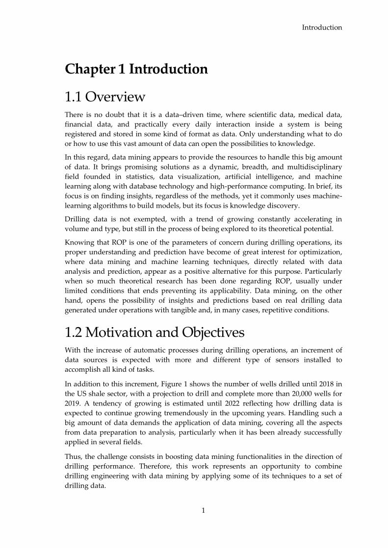
1.2 Motivation and Objectives With the increase of automatic processes during drilling operations, an increment of
data sources is expected with more and different type of sensors installed to
accomplish all kind of tasks.
In addition to this increment, Figure 1 shows the number of wells drilled until 2018 in
the US shale sector, with a projection to drill and complete more than 20,000 wells for
2019. A tendency of growing is estimated until 2022 reflecting how drilling data is
expected to continue growing tremendously in the upcoming years. Handling such a
big amount of data demands the application of data mining, covering all the aspects
from data preparation to analysis, particularly when it has been already successfully
applied in several fields.
Thus, the challenge consists in boosting data mining functionalities in the direction of
drilling performance. Therefore, this work represents an opportunity to combine
drilling engineering with data mining by applying some of its techniques to a set of
drilling data.
Introduction
2
Figure 1 Wells drilled, completed, and drilled-but-uncompleted per year until 2018.
Projection until 2022 (Jacobs, Journal of Petroleum Technology 2019)
The main objective is to improve the understanding of ROP behaviour, and when
possible identify the factors affecting its expected performance, with the creation of a
model to predict its response. The mean for this purpose are sensor data collected
constantly during normal drilling operations, along with geographical well position
data in one specific field.
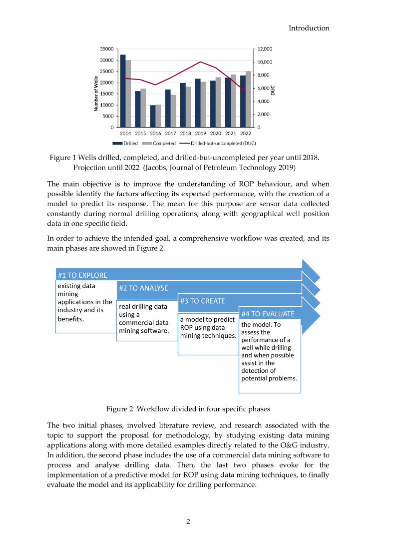
In order to achieve the intended goal, a comprehensive workflow was created, and its
main phases are showed in Figure 2.
Figure 2 Workflow divided in four specific phases
The two initial phases, involved literature review, and research associated with the
topic to support the proposal for methodology, by studying existing data mining
applications along with more detailed examples directly related to the O&G industry.
In addition, the second phase includes the use of a commercial data mining software to
process and analyse drilling data. Then, the last two phases evoke for the
implementation of a predictive model for ROP using data mining techniques, to finally
evaluate the model and its applicability for drilling performance.
#1 TO EXPLORE
existing data mining applications in the industry and its
benefits.
#2 TO ANALYSE
real drilling data using a commercial data mining software.
#3 TO CREATE
a model to predict ROP using data mining techniques.
#4 TO EVALUATE
the model. To assess the performance of a well while drilling and when possible assist in the detection of potential problems.
Data Mining
3
Chapter 2 Data Mining
2.1 Overview Data mining emerged during the late 1980s, with important advances through the next
decade and until today. It refers to the application of science to extract useful
information from large data sets or databases, focusing on issues relating to their
feasibility, usefulness, effectiveness, and scalability. In other words, a person, under a
particular situation, working with specific data sets and pursuing well-defined
objectives, executes it. (Gung 2016)
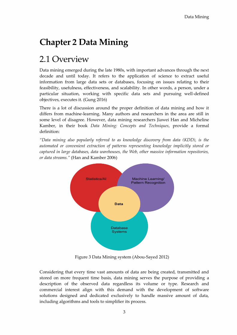
There is a lot of discussion around the proper definition of data mining and how it
differs from machine-learning. Many authors and researchers in the area are still in
some level of disagree. However, data mining researchers Jiawei Han and Micheline
Kamber, in their book Data Mining: Concepts and Techniques, provide a formal
definition:
“Data mining also popularly referred to as knowledge discovery from data (KDD), is the
automated or convenient extraction of patterns representing knowledge implicitly stored or
captured in large databases, data warehouses, the Web, other massive information repositories,
or data streams.” (Han and Kamber 2006)
Figure 3 Data Mining system (Abou-Sayed 2012)
Considering that every time vast amounts of data are being created, transmitted and
stored on more frequent time basis, data mining serves the purpose of providing a
description of the observed data regardless its volume or type. Research and
commercial interest align with this demand with the development of software
solutions designed and dedicated exclusively to handle massive amount of data,
including algorithms and tools to simplifier its process.
Data Mining
4
The term is not yet commonly used in the O&G industry; for that reason, some of its
functionalities and common applications should be shallow discussed to recognize its
value for the industry. There are two main tasks that can be performed using data
mining: descriptive and predictive. Descriptive tasks characterize the main features or
general properties of the data in a convenient way. The objective is to derive patterns,
which summarize the relationships in the data. On the other hand, predictive tasks
interpret the current data to model a future behaviour for some variables based on
values of other known variables.
To perform any of the tasks, a suite of techniques are employed. The selected approach
is highly depended on the nature of the task and the availability of the data. Some of
the techniques include Statistics, Artificial Intelligence (AI), Pattern Recognition,
Machine Learning, and Data Systems analysis.
2.2 Functionalities In order to be familiar with the terminology used in the framework of data mining, it is
important to properly segregate some common terms like model and pattern. A model
is a global concept that provides a full description of the data and can be apply to all
points in the database. On the other hand, a pattern corresponds to a local description
of some subset of the data that can hold for some variables, but not for all of them.
Patterns are used to extract unusual structures within the data and are valuable for
both main mining tasks. Then data mining techniques can be classified based on
different criteria like: the type of database to be mined, the type of knowledge to be
discovered, and the types of methods to be used. (Platon and Amazouz 2007)
Because it is a field in constant change, there are sort of best algorithms for certain
problems, and with pragmatic rules of thumb about when to apply each technique to
make it highly effective. Usually, a data mining system consists of a set of elements for
tasks such as characterization, association and correlation analysis, classification,
prediction, cluster analysis, outlier analysis, and evolution analysis. In addition, there
are a several variations of those tasks, resulting in new algorithms, considered in some
cases as “new techniques.” For the purpose of this thesis, only the broad classes of data
mining algorithms will be discussed. (Pinki, Prinima and Indu 2017)
2.2.1 Concept/Class Description: Characterization and
Discrimination Class/Concept description refers to the advantage of associating data with classes or
concepts for summaries of individual descriptions based on these precise terms.
There are three techniques used to derive this description:
Data Characterization: the class of interest, also referred as target class, is
summarized in general terms or, based on its features.
Data Discrimination: the general features of the class under study are compared
with the general features of one or more comparative classes, to obtain a
contrast between them.
Combination of both data characterization and discrimination.

Data Mining
5
The methods used for characterization and discrimination include summaries and
output presentations based on statistical measures, generalized relations, in rule forms
and descriptive plots like: bar charts, curves, pie charts, multidimensional tables, and
so on.
2.2.2 Frequent Patterns, Associations, and Correlations Frequent Patterns corresponds to one of the most basic techniques and is about
learning to recognize frequent patterns in data sets. It is usually based on
distinguishing aberrations in data happening at regular intervals over time. Different
kinds of frequent patterns include:
Frequent item-sets: denote a set of items that recurrently appear together in a
transactional data set.
Frequent sequential pattern: refer to a pattern occurring in a sub-sequential
trend, one after another, repeatedly.
Frequent sub-structured pattern: occur when different structural arrangements
take place on a regular basis. The form of those arrangements can be graphs,
trees or lattices, and may be combined with sub-sequences or item-sets.
Associations and correlations occur when frequent patterns within the data are tracked
in a more specific way to dependently link variables. In the association analysis, two
groups can be distinguished related to the number of attributes/dimensions:
Single-dimensional association rule: Involves a single attribute or predicate
that repeats (i.e., buy)
Multidimensional association rule: Consists of more than one attribute or
predicate (i.e., age, income, and buy).
When certain association rules are considered interesting, statistical correlations can be
applied to show whether and, how strongly associated attribute–values pairs relate.
2.2.3 Classification and Prediction A more complex and commonly applied mining technique is classification, where a
model is created to describe and differentiate data classes/concepts and then collect
them together into discernable categories. The final aim is to use the model, derived
from the known data, also known as ‘training data’, to make predictions of the data
labelled as unknown.
There are a number of forms to represent the model, for example using:
Classification rules: with the function IF – THEN.
Decision trees: creating a flow chart via an algorithm based on the “information
gain” of the attributes. Basically, each node is tested on an attribute value,
where the tree brands represent the outcome and the leaves denote the class
distribution.
k-nearest neighbour (k-NN) classification: uses the data to determine the model
structure by not making assumptions on the original data distribution (non-
parametric) but learning based on feature similarity. Hence, it does not do
Data Mining
6
generalization based on the training data rather it utilizes the training data for
the testing phase.
Neural networks: structurally consist of many small units called neurones, and
it is a powerful mathematical tool for solving problems. The neurons are linked
to each other into layers, and cooperate to propagate the inputs using weighted
connections through ‘activation functions’. Then the Bias values are converted
mathematically to continue the transformation of the inputs into outputs in the
best possible manner. (Solesa 2017)
Support Vector Machine: combines linear modelling and instance-based
learning to overcome the limitations of linear boundaries. It relies in selecting a
small number of critical boundary instances, called support vectors from each
class, and build a linear discriminant function that separates them as widely as
possible. The result permits the inclusion of extra nonlinear terms in the
function, in order to form higher-order decision boundaries. (Witten and Frank
2005)
Naïve Bayesian: it’s based on the Bayes’s rule (named after Rev. Thomas Bayes
1702-1761) and is mainly appropriate when the dimensionality of the inputs is
high, i.e., in a simplistic way, it assumes independency between attributes. This
technique works well when combined with procedures to eliminate
redundancy (non-independent attributes). The algorithm output will be a
function of the prior probability, based on previous experience, and the
likelihood for a new object to be classified in a certain class. Naïve Bayes
miscarries if a particular attribute value does not occur in the training set along
with every class value. (Witten and Frank 2005)
Though conventionally the term prediction is used in reference to numeric prediction
as class label prediction, more precisely, classification is used for categorical
predictions labels (discrete, unordered), and prediction to emphasize models
describing continuous-valued functions. In this context, regression analysis appears as
a statistical methodology, commonly used for numeric prediction. However, other
methods exist and could also provide a good performance.
2.2.4 Outlier Detection In many cases, data sets may include anomalies, or outliers, i.e., data that do not
comply with the general behaviour or model of the data, data that need to be identified
and demand investigation to get a clear understanding of the data set. In general, data
mining offers algorithms to discard outliers as noise or exceptions. This type of data
could affect data analysis and therefore, needs to be excluded.
This functionality can also serve other purpose, when anomalies can provide
information of interest, like for example, in cases of fraud detection using credit cards
to purchase extremely large amounts compare to regular transactions.
Outlier detection is possible conventionally through statistical tests, where a certain
type of distribution is assumed, or by using probability models to discard anomalies.
Other methods include the use of distance or density measures, where examples
substantially far or with less data density from any other cluster are identified as
Data Mining
7
outliers. On the other hand, deviation-based methods, compare the main
characteristics between examples and by examining the differences set apart outliers.
2.2.5 Cluster Analysis Clustering seems similar to classification, but involves grouping amounts of data
without a specific known class label, using only their similarities. Clustering, can in
fact, be used to generate the necessary labels.
The principle used to group the data search for examples to maximize their intraclass
similarities within the group, and at the same time, to minimize the intraclass
similarities with other groups. The final result is different groups (clusters) in a way
that examples in the same group are similar to each other but different from examples
in other groups. Groups are clearly distinguished and can be used to derive rules. (Han
and Kamber 2006)
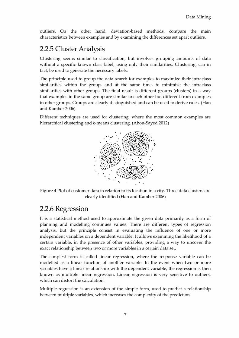
Different techniques are used for clustering, where the most common examples are
hierarchical clustering and k-means clustering. (Abou-Sayed 2012)
Figure 4 Plot of customer data in relation to its location in a city. Three data clusters are
clearly identified (Han and Kamber 2006)
2.2.6 Regression It is a statistical method used to approximate the given data primarily as a form of
planning and modelling continues values. There are different types of regression
analysis, but the principle consist in evaluating the influence of one or more
independent variables on a dependent variable. It allows examining the likelihood of a
certain variable, in the presence of other variables, providing a way to uncover the
exact relationship between two or more variables in a certain data set.
The simplest form is called linear regression, where the response variable can be
modelled as a linear function of another variable. In the event when two or more
variables have a linear relationship with the dependent variable, the regression is then
known as multiple linear regression. Linear regression is very sensitive to outliers,
which can distort the calculation.
Multiple regression is an extension of the simple form, used to predict a relationship
between multiple variables, which increases the complexity of the prediction.
Data Mining
8
Some of the most popular types of Regression are Logistic Regression, Polynomial
Regression, Stepwise Regression, Ridge Regression, Lasso Regression, among others.
Each one following specific conditions to better suits problems (Ray 2015).
2.3 Common Applications Data mining is widely popular in credit risk applications and in cases of fraud
detection. The common technique applied is Classification, where a model is
developed employing pre-classified examples and then categorize the records through
decision tree or neural network-based classification algorithms. Outlier detection is
also used for fraud detection, where the outliers become the data of interest. In general,
during the process, it is necessary to include records of valid and fraudulent activities
to properly train the model on how to determine the required parameters to do the
discrimination. (Pinki, Prinima and Indu 2017)
Data mining is also being used successfully in industrial process applications, in areas
that include process monitoring, fault detection and diagnosis, process-related
decision-making support to improve process understanding, soft sensors, process
parameter inference, and many others. Each application demands different techniques
along with different types of data bases. However, one of the most popular techniques
for prediction modelling is based on neural network approaches due to its well-known
predictive capabilities. In some cases, a combination of various methods can also be
used to create hybrid models and overcome individual limitations to achieve the
proposed objective. (Platon and Amazouz 2007)
Retailer analysis of buying patterns is another classical application of data mining,
where its solving problems proficiency of analysing long time stored databases full of
data of customer actions and loyalty represents an open door for the marketplaces. In
every transaction, customers expose their choices, along with some of their profile
data, that when properly processed results in patterns of customer behaviour. This
information allows to identify distinguishing characteristics related to their loyalty and
churn likelihood to certain products. The results provide client’s profile identification
and clients preferences that can be worked as inputs for marketing strategies, market
predictions, to serve a customer oriented economy where increasing sales is the final
aim. As an example, the giant Wal-Mart can be cited, which transfers all its relevant
daily transactions to a data warehouse collecting terabytes of data, that is also
accessible to its suppliers enabling them to extract the information regarding customer
buying patterns and shopping habits, as well as most shopped days, most sought for
products, and so on.
There are many other specific applications. Like screening images with a hazard
detection system to identify oil slicks from satellite images and give an earlier warning
of ecological disasters. For the forecast of the load for the electricity supply industry
based on historical records of consumption. In the medicine field, for best treatment
selection and in human in vitro fertilization where over 60 recorded features of the
embryos need to be analysed simultaneously; and countless more applications. (Witten
and Frank 2005)
Data Mining
9
2.4 Applications in the Industry It has been estimated that a large offshore field delivers more than 0.75 terabytes of
data weekly, and a large refinery 1 terabyte of raw data per day. References have been
made to input/output points somewhere between 4000 and 10000 per second. (Abou-
Sayed 2012) With this amount of data flowing constantly, the key lies in ensuring that
the right information reaches the right people at the right time.
The industry’s emphasis has been normally on monitoring and assurance of
production; therefore, some Operators and Service Companies recognizing the
potential of data mining have started to make important investments in that direction.
Some examples of the potential of data mining that are already applied to optimize
solutions are related to:
Predict well productivity, reservoir recovery factors, and decline rate.
Identify key drivers for performance of producers and water injectors subjected to
multiple factors like high pressures and temperature.
Defining best practices in completion.
Minimizing production downtime and well intervention costs.
Extend production life of wells.
Data Mining scope is still uncertain. Therefore some interesting advances are further
discussed showing it application in three different disciplines. The first example refers
to Reservoir Management and how supported on seismic data it is possible to identify
and advice regarding sweet spots. The second example is related to Wellbore stability,
and how data can be used to prevent some of the causes and the associated risks. In the
last case, an application for Formation Evaluation predictions is presented as an
alternative to reduce completion costs.
2.4.1 Example 1 - Reservoir Management British Petroleum (BP) along with Beyond Limits are working on a project to absorb the
learnings of petrotechnical experts, like geologists and petroleum engineers, using
cognitive computing to imitate their decision-making processes as they work on
subsurface challenges.
The first joint program is already running since July-2018 with a group of BP’s
upstream engineering team aiming that their expertise train the system and remain
longer digitally. It was meant to be used on the job, in a way that a number of Artificial
Intelligent (AI)-agents constantly interact with members of the team to start building
experience, learn the art of solving problems and store knowledge further. It starts as a
design tool, with a process of learning to become a recommendation tool that with
experience can build trust, to later be used as a control system. In a glimpse of the early
stage of the project, BP is expecting from the system answers on how to mitigate the
impact of sand production with prediction and advice with asphaltene buildups in a
well.
A cognitive computing system involves self-learning technologies that use basic
analytics, deep learning, data mining, pattern recognition, and natural language
Data Mining
10
processing to solve problems the way humans solve problems, by thinking, reasoning
and remembering. It can combine data from different information sources, weigh its
context, and solve conflicts using the evidence to propose the best possible answers.
Through deep learning, the information is processed in layers where the output from
one layer becomes the input for the next one, improving the result. (Jacobs, Journal of
Petroleum Technology 2018)
BP’s interest on Beyond Limits arose due to its work with Jet Propulsion Laboratory
(JPL) on the real Mars rovers Curiosity. One of their principals was the author of a
distinctive AI program in charge of managing one of the rover’s battery. The
outstanding was that when the program detected that the solar panels were suffering
from dust storms, it autonomously accessed data from pressure and temperature
sensors with the purpose of building a weather model in order to understand how to
properly orient its solar panels to prevent dust from storms. This aligns with the
definition of AI as “the science of making computers do things that require intelligence
when done by humans” (Evans 2017). In the Curiosity mission, the program was
capable to execute a task that was not designed in its model.
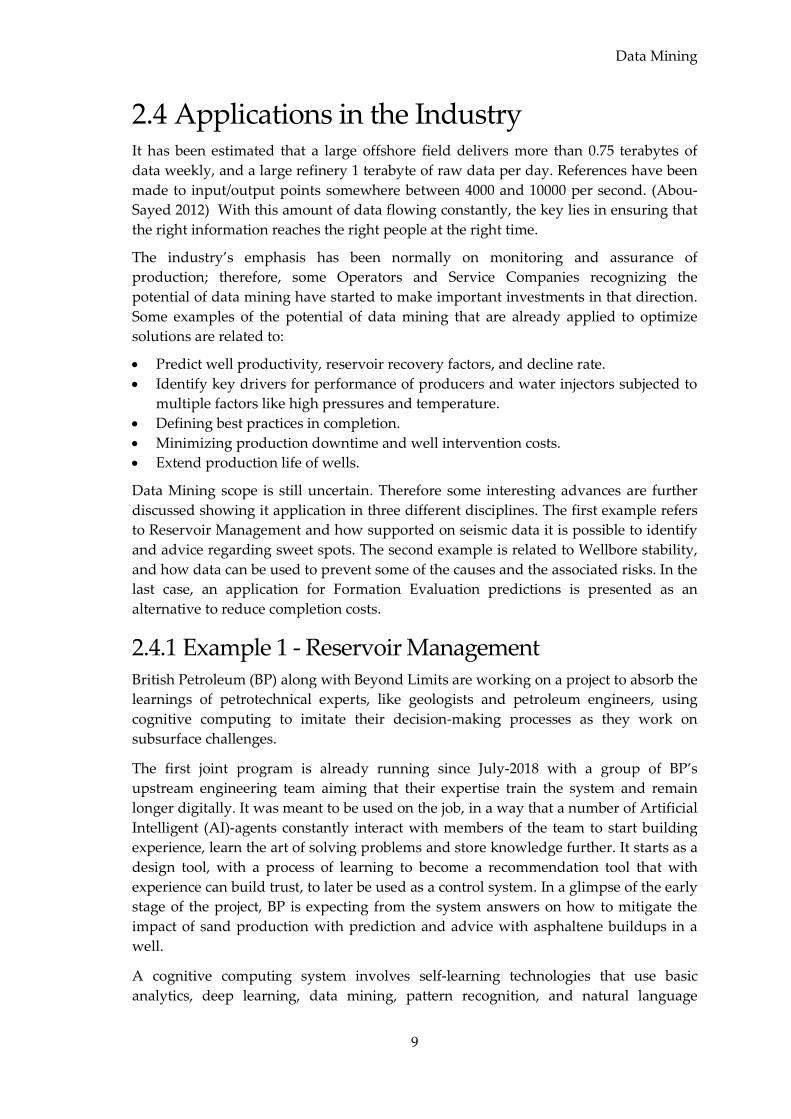
Beyond Limits is relatively new and not exclusive to the Oil & Gas industry, therefore
unknown. However, it is developing a system, referred as Reservoir Management
advisor, that will learn from geologists and reservoir engineers as they search for sweet
spots in offshore seismic data to recommend probable well locations, and the more
suitable well designs to maximize the recovery of hydrocarbons. It is supported on
another software called Sherlock IQ, born from the experience on the rover program
and based on machine cognition to autonomously shift through different paths of data
to discover specific details and scenarios that ultimately will allow it to assess risks. It
is expected to become reliable, faster, and capable to appraise more data in a period of
just few hours, to complement the work of real experts, which usually can take months.
Figure 5 Beyond Limits Reservoir Management advisor (Jacobs, Journal of Petroleum
Technology 2018)
Data Mining
11
2.4.2 Example 2 – Data Mining to Understand Drilling
Conditions. Lately terminologies like “intelligent wells” or “digital oilfields” are becoming more
and more oft used, according to how data use is changing in the industry. The usual
approach of established workflows using only specific set of relationships between
variables, like linking core data to well logs, has become obsolete.
Data mining functionality along with the proper technology allow to work with
disparate data types structured and unstructured, and with different degrees of
accuracy and granularity. The combination enables rapid associations between data
that normally would be assumed not linked. This perspective was tested by the UK
Department of Energy & Climate Change, with a project together with CGG as the
official UK Continental Shelf data release agent. The study purpose was to improve
drilling results using data mining main tasks: descriptive modelling and predictive
relationships. More specifically the project’s aim was to find out the optimum
conditions for drilling efficiency and identify the high-risk situations.
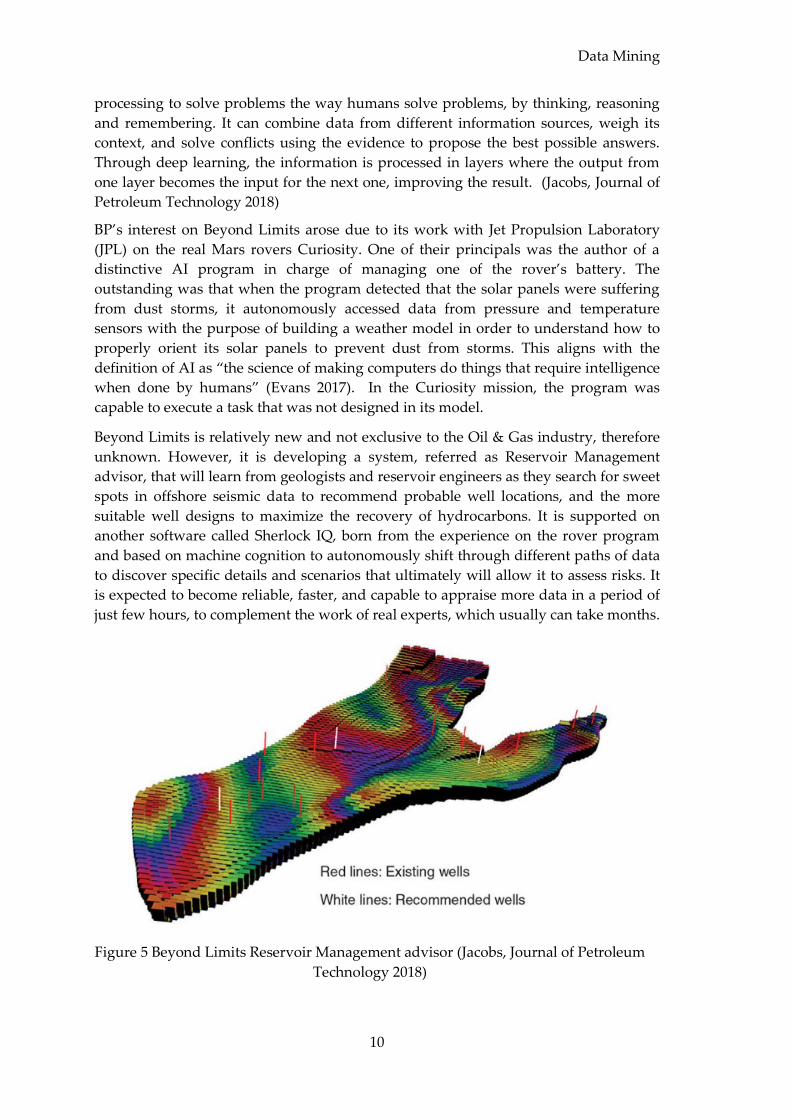
A total of 350 wells located in the UK North Sea were used for the study in the form of
20000 files with different formats but including data from Well logs, well geographical
locations, drilling parameters, geological reports, and well deviations. All data was
thoroughly loaded, quality controlled and finally used for the analysis. The caliper
reading was determined as the main reference, to identify poor hole conditions, by
normalizing it with the bit size. Other drilling parameters in detail used were: Torque,
Weight on Bit (WOB), and ROP. The visualization tool allowed to combine and
contrast the inputs/variables in order to understand how its variations affect borehole
quality. (Johnston and Aurelien 2015)
Figure 6 Anomaly Detection: A high risk situation was identified (Johnston and
Aurelien 2015)
Data Mining
12
Data mining revealed its functionality working with big amount of data and
performing better than the usual approach and in very short period. Figure 6, is an
example of how anomaly detection was possible using one of the visualization tools. It
showed the case of a single well well where an increase of WOB, ended in poor hole
conditions and affecting the reading of the caliper measurement. Subsequently, it was
found that the well faced logging stuck issues and forced an extra wiper trip. In
conclusion, a high risk situation was identified.
There were more discoveries as result of the study, which included some predictive
statistics meant to provide valuable information to drill future wells in the same area
hopefully with less problems.
2.4.3 Example 3 – Predictions of Formation Evaluation
Measurements to Replace Logging Tools used in Lateral
Sections. The shale revolution growth over the past two decades positioned United States in the
top of oil producers worldwide, competing with Saudi Arabia and Russia (Donnelly
2019). However, the threat of the low oil price market after the crisis at the end of 2014,
forced producers to become extremely efficient, to cut costs, and to look for innovation.
In this regard, in the Eagle Ford Shale in Texas, the EOG Resources reported a decrease
of 70% in the average drilling days from 14.2 during 2012 to 4.3 in 2015. The curios side
of this improvement in efficiency relates to the overall cost per well, which only
decreased a 20%, from USD 7.2 million to USD 5.7 million. The discrepancy is due to
the completion cost, being the major contributor and independent of any possible
improvement in efficiency during operations (Parshall 2015). Innovation was on
demand.
It is important to bear in mind that to provide smart completions, the location of stages
and perforation clusters is essential and currently engineering designed using
formation evaluation technology. This technology, known by being costly, must be add
to the already considerable cost per stage, where experience has shown that between
30% and 50% of the perforation clusters do not even produce. This situation caught the
attention of Quantico Energy Solutions, a data driven company, understanding the
need of more and better information about the reservoirs and its geological complexity
without the investment required by conventional logs.
The necessity of innovation became stronger due to the way shale fields are developed
where operators can afford to log few appraisal wells but not all the subsequent wells,
which ideally should be smartly completed too. Therefore, data mining became an
alternative, considering a scenario where already thousands of wells in the area have
been drilled, collecting not just important geological data from logging tools and
cutting samples, but also a huge amount of data regarding drilling parameters,
completion and production.
After a two years research, Quantico Energy Solutions, supported by several major
shale operators, along with industry specialist in neural networks and openhole
logging tool designers, developed a source of formation evaluation characteristics,
Data Mining
13
called QLog. It is a commercial logging system based on machine-learning software
that trained neural networks models using the drilling and logging data from
horizontal wells collected for years by operators. It is capable to simulate
compressional, shear, and density logs on horizontal wells to prevent the use of
expensive logging tools. With the results, it is possible to derive elastic properties such
as Young’s modulus, Poisson’s ratio, horizontal stress, and brittleness, fundamental to
engineer the completions. Actually, later on, the company developed QFrac software,
which using the simulated results, is able to recommend engineered stage locations.
The success of the system, requiring less investment compared to the actual design and
test of physical logging tools, created a network effect where more operators decided
to step in, providing more data. In consequence, a real time simulator service was
developed, QDrill, to assist drillers with well placement operations too. It is a software
based on artificial intelligence, that provides petrophysical properties of a reservoir.
The algorithm was developed using several hundred wells for many basins that have
the measured well logs along with the drilling data. It was designed to use as input,
gamma ray logs and drilling dynamics parameters, like ROP, WOB, torque, and so on.
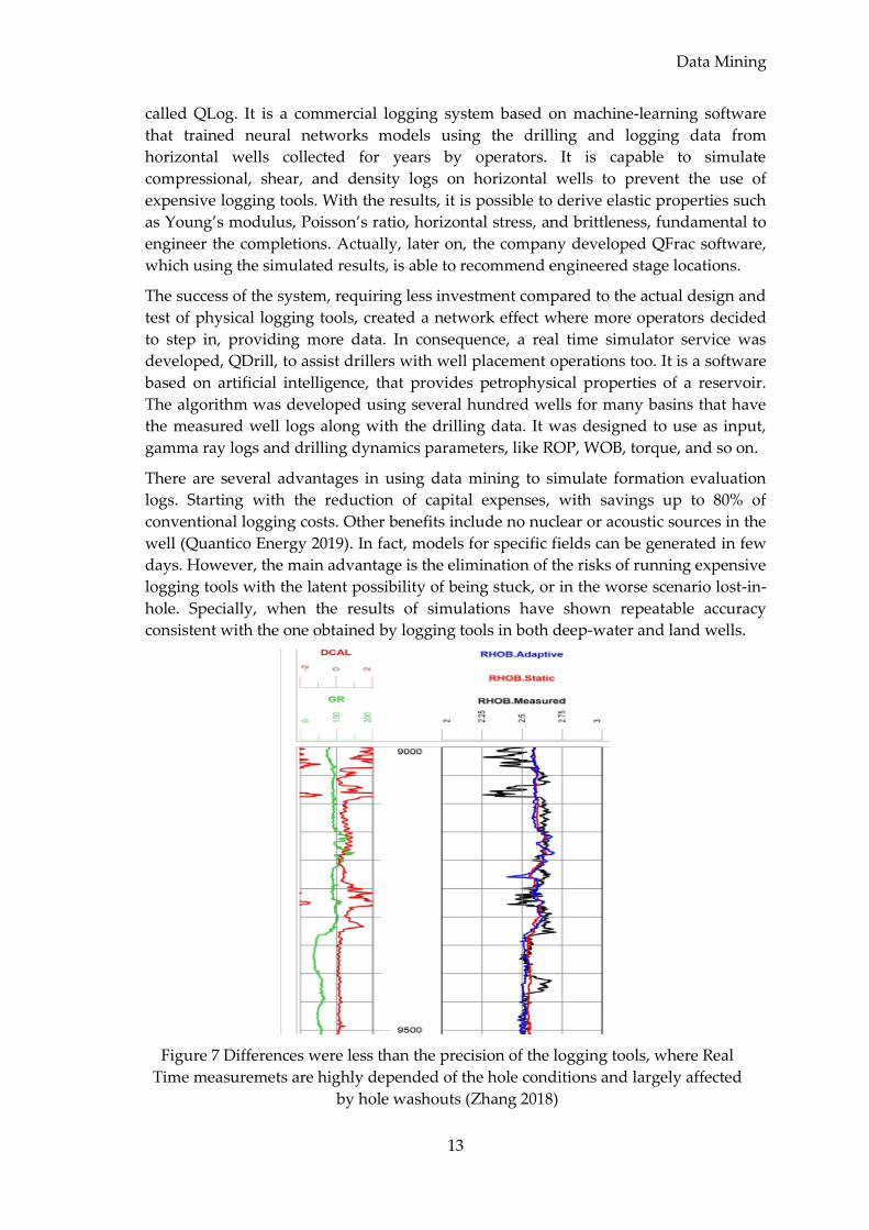
There are several advantages in using data mining to simulate formation evaluation
logs. Starting with the reduction of capital expenses, with savings up to 80% of
conventional logging costs. Other benefits include no nuclear or acoustic sources in the
well (Quantico Energy 2019). In fact, models for specific fields can be generated in few
days. However, the main advantage is the elimination of the risks of running expensive
logging tools with the latent possibility of being stuck, or in the worse scenario lost-in-
hole. Specially, when the results of simulations have shown repeatable accuracy
consistent with the one obtained by logging tools in both deep-water and land wells.
Figure 7 Differences were less than the precision of the logging tools, where Real
Time measuremets are highly depended of the hole conditions and largely affected
by hole washouts (Zhang 2018)

Data Mining
14
Figure 7, refers to a case study in the Midcontinent region of the U.S., where the target
was a formation with a clastic laminated/layered sandstone reservoir. The AI model
was prepared and the client drilled two laterals sections using Quantico logs for real
time geosteering interpretations to place completion stages in areas with higher
porosity intervals and equalizing minimum horizontal stress across stages. To compare
predicative accuracy and repeatability of the model with the real time measurements,
two models were used: one static, based on information from proprietary database,
and one adaptive, constantly incorporating in the training set the data acquired from
logging tools. The results showed negligible differences between the bulk densities
from both models in relation to the one measured by logging tools (Zhang 2018).
Measurements and Data
15
Chapter 3 Measurements and Data
The first step in data mining consist in gathering all relevant data for the study, which
might not be an obvious task. This is why it is important to state a clear objective to
identify the necessary data. In this regard and, as earlier mentioned, the aim for this
work looks for a better understanding of the ROP measurement, which in operations is
the reflection of the drilling conditions, and include among others, the drilling
parameters set while drilling. Thus, prior to mining the data, it is key to understand
which are the main measurements and sensors involved during drilling operations and
providing the data, as well as some relevant concepts and considerations regarding the
data itself.
3.1 Sensors and Rate of Penetration
3.1.1 Sensors Measurements There are different number and type of sensors involved during normal drilling
operations. This is highly related to the nature of the rig, the sort of operation, and the
available budget. Sensors are used in the process to measure parameters, and their
outputs are the values that provide these parameters’ descriptions.
It is important to distinguish how some measurements are originated with sensors
installed on surface while others come from downhole sensors included in the tools
used in the Bottom Hole Assembly (BHA). In addition, there are different types of
measurements, some are direct and others indirect. Finally, two domains are working
in parallel, so data measurements are acquired in Time and Depth.
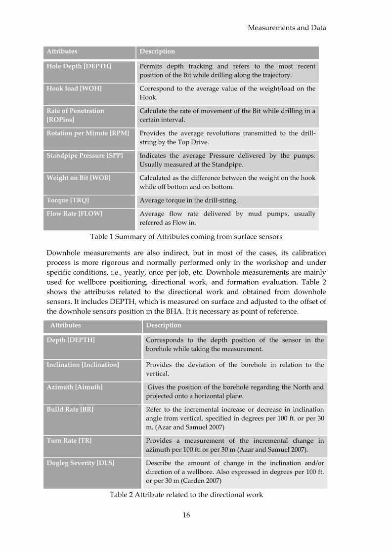
In general, there are more less 10 key measurements obtained from surface sensors.
However, due to the scope of the present work, only some of the main and most
common measurements will be discussed, as they provide input for further analysis
and modelling. Table 1 summarizes the surface sensor measurements, normally
acquired by the mud logging service provider during daily drilling operations, with a
brief description for each attribute (Nguyen 1996).
As previously mentioned, data is acquired in two domains, being DEPTH one of them;
for that reason, this attribute is by far the most important one regarding measurements.
Nevertheless, concerning rig operations, there are three measurements that are
indispensable for operations: hook load, rotation and pump discharge pressure.
Besides, the majority of these measurements are indirect, demanding a certain level of
interpretation along with regular on site calibration and thus more susceptible to
human error.
Measurements and Data
16
Attributes Description
Hole Depth [DEPTH] Permits depth tracking and refers to the most recent
position of the Bit while drilling along the trajectory.
Hook load [WOH] Correspond to the average value of the weight/load on the
Hook.
Rate of Penetration
[ROPins]
Calculate the rate of movement of the Bit while drilling in a
certain interval.
Rotation per Minute [RPM] Provides the average revolutions transmitted to the drill-
string by the Top Drive.
Standpipe Pressure [SPP] Indicates the average Pressure delivered by the pumps.
Usually measured at the Standpipe.
Weight on Bit [WOB] Calculated as the difference between the weight on the hook
while off bottom and on bottom.
Torque [TRQ] Average torque in the drill-string.
Flow Rate [FLOW] Average flow rate delivered by mud pumps, usually
referred as Flow in.
Table 1 Summary of Attributes coming from surface sensors
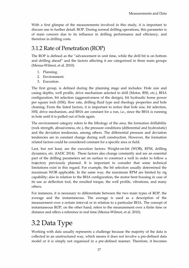
Downhole measurements are also indirect, but in most of the cases, its calibration
process is more rigorous and normally performed only in the workshop and under
specific conditions, i.e., yearly, once per job, etc. Downhole measurements are mainly
used for wellbore positioning, directional work, and formation evaluation. Table 2
shows the attributes related to the directional work and obtained from downhole
sensors. It includes DEPTH, which is measured on surface and adjusted to the offset of
the downhole sensors position in the BHA. It is necessary as point of reference.
Attributes Description
Depth [DEPTH] Corresponds to the depth position of the sensor in the
borehole while taking the measurement.
Inclination [Inclination] Provides the deviation of the borehole in relation to the
vertical.
Azimuth [Aimuth] Gives the position of the borehole regarding the North and
projected onto a horizontal plane.
Build Rate [BR] Refer to the incremental increase or decrease in inclination
angle from vertical, specified in degrees per 100 ft. or per 30
m. (Azar and Samuel 2007)
Turn Rate [TR] Provides a measurement of the incremental change in
azimuth per 100 ft. or per 30 m (Azar and Samuel 2007).
Dogleg Severity [DLS] Describe the amount of change in the inclination and/or
direction of a wellbore. Also expressed in degrees per 100 ft.
or per 30 m (Carden 2007)
Table 2 Attribute related to the directional work
Measurements and Data
17
With a first glimpse of the measurements involved in this study, it is important to
discuss one in further detail: ROP. During normal drilling operations, this parameter is
of main concern due to its influence in drilling performance and efficiency, and
therefore in drilling costs.
3.1.2 Rate of Penetration (ROP) The ROP is defined as the “advancement in unit time, while the drill bit is on bottom
and drilling ahead” and the factors affecting it are categorized in three main groups
(Mensa-Wilmot, et al. 2010):
1. Planning.
2. Environment.
3. Execution.
The first group, is defined during the planning stage and includes: Hole size and
casing depths, well profile, drive mechanism selected to drill (Motor, RSS, etc.), BHA
configuration, bit selection (aggressiveness of the design), bit hydraulic horse power
per square inch (HSI), flow rate, drilling fluid type and rheology properties and hole
cleaning. From the listed factors, it is important to notice that hole size, bit selection,
HSI, drive mechanism, and BHA are constant for a run, i.e., since the BHA is running
in hole until it is pulled out of hole again.
The environment category refers to the lithology of the area, the formation drillability
(rock strength, abrasiveness, etc.), the pressure conditions (differential and hydrostatic)
and the deviation tendencies, among others. The differential pressure and deviation
tendencies are in constant change during well construction. However, the formation
related factors could be considered constant for a specific area or field.
Last, but not least, are the execution factors: Weight-on-bit (WOB), RPM, drilling
dynamics, etc. (IADC 2014). These factors also change constantly and are an essential
part of the drilling parameters set on surface to construct a well in order to follow a
trajectory previously planned. It is important to consider that some technical
limitations exist in this regard. For example, the bit selection usually determined the
maximum WOB applicable. In the same way, the maximum RPM are limited by rig
capability; also in relation to the BHA configuration, the motor bent housing in case of
its use as deflection tool, the resulted torque, the well profile, vibrations, and many
others.
For instances, it is necessary to differentiate between the two main types of ROP, the
average and the instantaneous. The average is used as a description of the
measurement over a certain interval or in relation to a particular BHA. The concept of
instantaneous ROP, on the other hand, refers to the measurement over a finite time or
distance and offers a reference in real time (Mensa-Wilmot, et al. 2010).
3.2 Data Type Working with data usually represents a challenge because the majority of the data is
collected in an unstructured way, which means it does not involve a pre-defined data
model or it is simply not organized in a pre-defined manner. Therefore, it becomes
Measurements and Data
18
important to understand how to work with different data sets based on the final aim.
By definition “an attribute is a property or characteristic of an object, that may vary,
either from one object to another or from one time to another” (Tan, Steinbach and
Kumar 2006). The description of data is done by using different attributes, which not
only differ in its values but might also vary in its type.
At the most basic level, the physical value for different attributes are mapped as
numbers or symbols, where the values used to represent an attribute may have
properties that are not properties of the attribute itself, and vice versa. A way to
differentiate the types of attributes is to recognise the properties of numbers associated
to the properties of the attribute. Four main operations are used to distinguish between
attributes:
1. Distinctness.
2. Order.
3. Addition.
4. Multiplication.
Resulting in four types of attributes, with specific properties and operations clearly
defined and valid for each type (Tan, Steinbach and Kumar 2006):
1. Nominal: Provide enough information to distinguish one object from another
(=, ≠). For example, gender, ID numbers, etc.
2. Ordinal: Based on the information objects can be ordered with a logic criteria (<,
>). For example, grades, costs, quality, etc.
3. Interval: The differences between values are meaningful (+, -). For example,
temperature in Celsius or Fahrenheit, where a unit of measurement exists.
4. Ratio: The differences and ratios between values are meaningful. For example,
monetary quantities, age, length, etc.
The first and second type of attribute are commonly denoted as categorical or
qualitative, and cannot be treated as numbers, even if represented by numbers, because
of its absence of the properties of numbers. In contrast, the last two types of attributes
are usually referred to as quantitative or numeric, and are not only represented by
numbers but actually, those numbers have direct meaning as measurement and have
most of the properties of numbers.
In addition, attributes can also be classified based on their numeric values, which can
be discrete or continuous. Discrete attributes are usually represented using integer
variables and have a finite set of values, i.e., can only take certain values. A special
subgroup of discrete attributes is binary attributes, where only two values are possible
(0 or 1, True or False, etc.) and often represented as Boolean variables. Continuous
attributes are essentially real numbers, can occupy any value over a continuous range
and are represented as floating-point variables. Normally, categorical attributes are
discrete, while numeric attributes are continuous.
Measurements and Data
19
3.3 Data Issues, Limitations and Resource
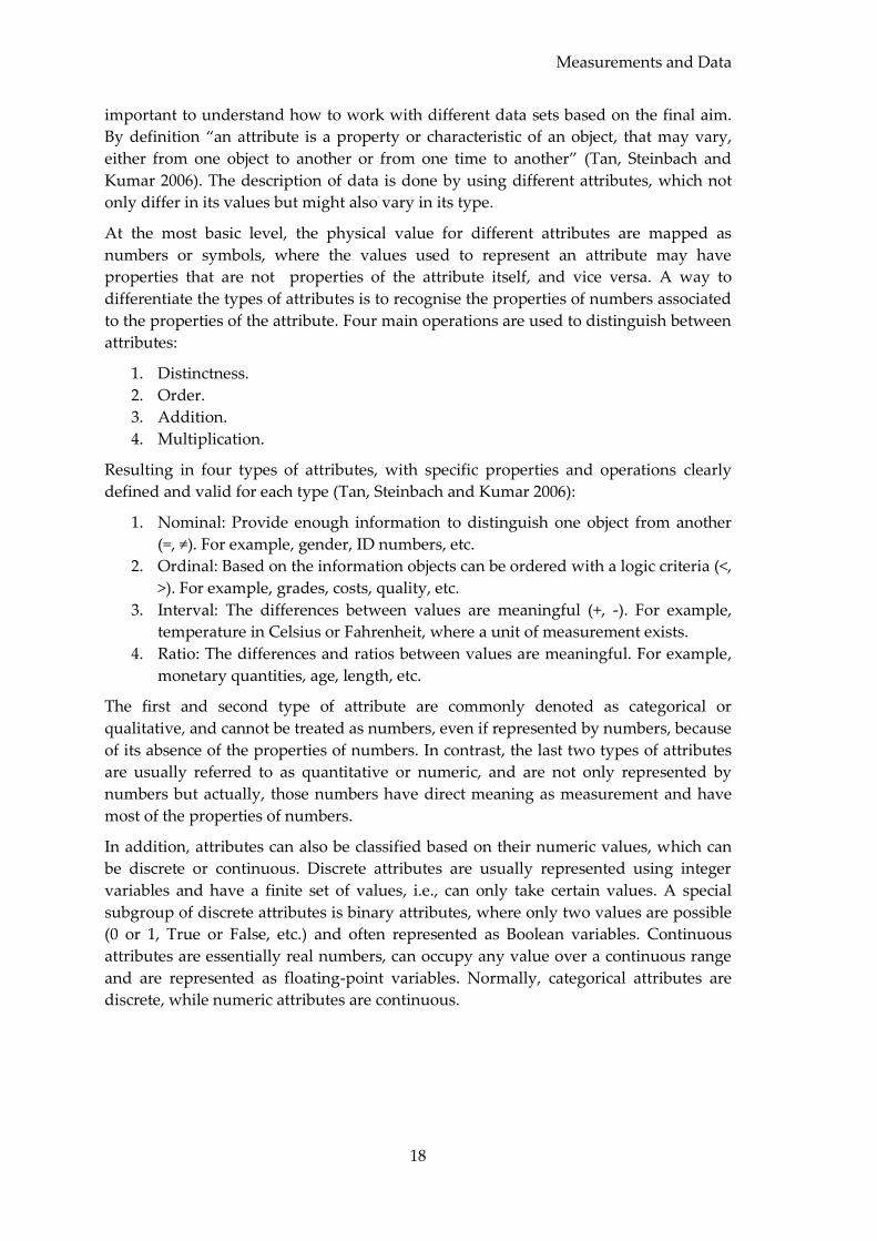
Constraints The most time consuming stage during any application of data mining corresponds to
the preparation of the data for processing. This includes collecting and cleaning the
data. Surveys show that between 60 to 80% of the time is designated to this purpose.
Figure 8 Results of survey between data scientists showing the time needed to
massage the data prior its use (Press 2016)
There are several measurements and data collection issues. Mainly, related to human
error, limitation of measuring devices, or defects in the data collection process, which
includes inappropriate sensor installation or poor understanding of the physics
involved behind the measurement (Maidla, et al. 2018). Therefore, it is very common to
find missing data, duplicate objects, outliers, and inconsistent values.
Typical errors during the measurement process result in differences between the
recorded value and the true value, which is known as discrepancy. This can happen
due to several reasons like a sensor defect, the used of wrong calibrations or an
inadequate installation. Other common problems involve facing noise in the signal or
simply lack of maintenance, allowing debris or humidity to affect the measurement.
Signal noise is normally associated with spatial or temporal components that result in
spiking signals distorting the measurement (Tan, Steinbach and Kumar 2006).
Errors concerning the data collection process include omitting relevant data or the
inappropriate inclusion of data, which is not suitable for the analysis. Moreover, lack of
availability of data. Finally, yet importantly, data frequency and range must as well be
considered, because it can affect the granularity of the data, having an impact on the
results.
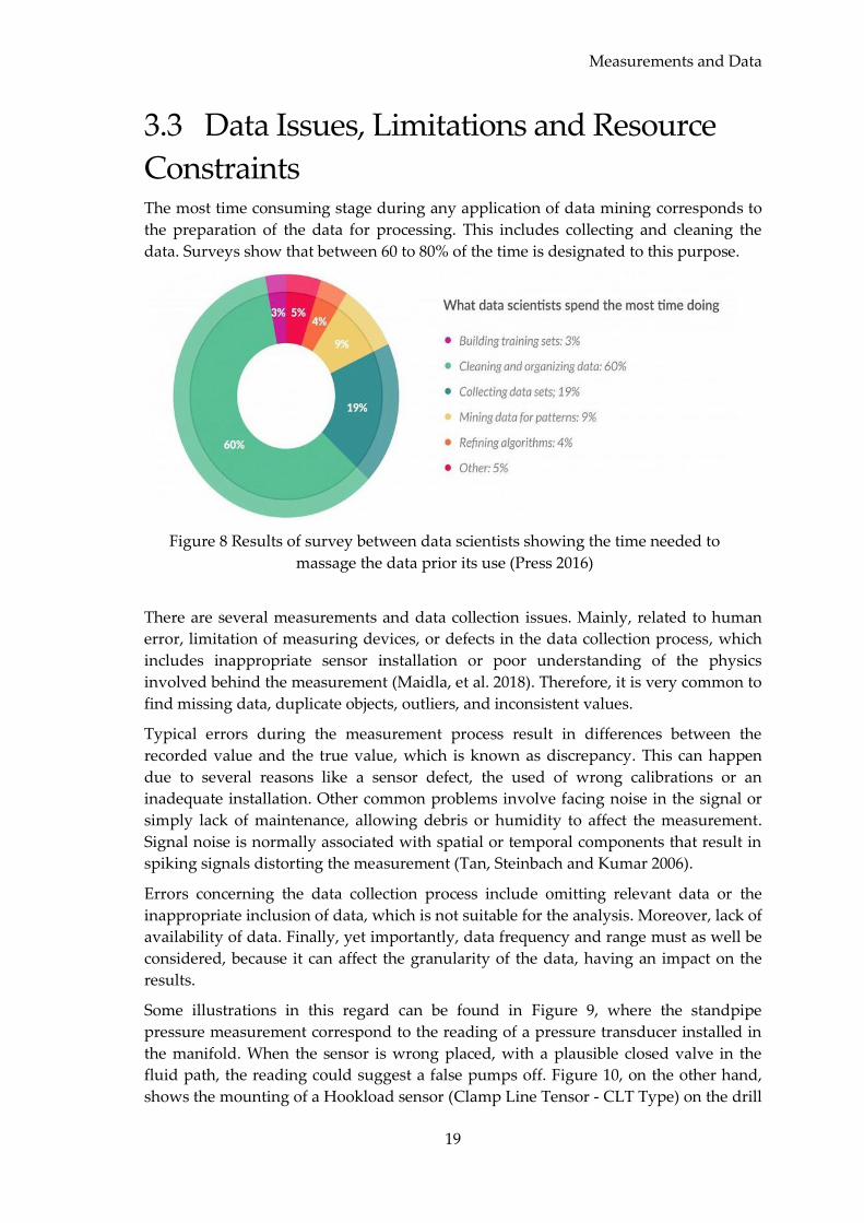
Some illustrations in this regard can be found in Figure 9, where the standpipe
pressure measurement correspond to the reading of a pressure transducer installed in
the manifold. When the sensor is wrong placed, with a plausible closed valve in the
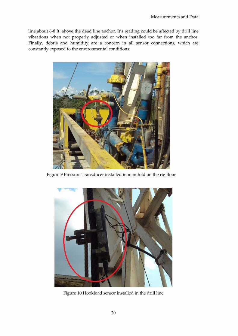
fluid path, the reading could suggest a false pumps off. Figure 10, on the other hand,
shows the mounting of a Hookload sensor (Clamp Line Tensor - CLT Type) on the drill
Measurements and Data
20
line about 6-8 ft. above the dead line anchor. It’s reading could be affected by drill line
vibrations when not properly adjusted or when installed too far from the anchor.
Finally, debris and humidity are a concern in all sensor connections, which are
constantly exposed to the environmental conditions.
Figure 9 Pressure Transducer installed in manifold on the rig floor
Figure 10 Hookload sensor installed in the drill line
Methodology
21
Chapter 4 Methodology
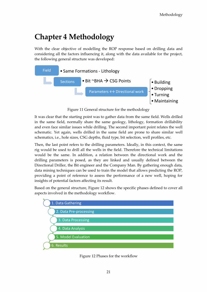
With the clear objective of modelling the ROP response based on drilling data and
considering all the factors influencing it, along with the data available for the project,
the following general structure was developed:
Figure 11 General structure for the methodology
It was clear that the starting point was to gather data from the same field. Wells drilled
in the same field, normally share the same geology, lithology, formation drillability
and even face similar issues while drilling. The second important point relates the well
schematic. Yet again, wells drilled in the same field are prone to share similar well
schematics, i.e., hole sizes, CSG depths, fluid type, bit selection, well profiles, etc.
Then, the last point refers to the drilling parameters. Ideally, in this context, the same
rig would be used to drill all the wells in the field. Therefore the technical limitations
would be the same. In addition, a relation between the directional work and the
drilling parameters is posed, as they are linked and usually defined between the
Directional Driller, the Bit engineer and the Company Man. By gathering enough data,
data mining techniques can be used to train the model that allows predicting the ROP,
providing a point of reference to assess the performance of a new well, hoping for
insights of potential factors affecting its result.
Based on the general structure, Figure 12 shows the specific phases defined to cover all
aspects involved in the methodology workflow.
Figure 12 Phases for the workflow
Field • Same Formations - Lithology
Sections • Bit ~BHA CSG Points
Parameters ↔ Directional work
• Building
• Dropping
• Turning
• Maintaining
1. Data Gathering
2. Data Pre-processing
3. Data Processing
4. Data Analysis
5. Model Evaluation
6. Results
Methodology
22
In the following sections, only the first four phases of the workflow will be explained
in detail, and the other ones will be covered in the next chapter.
4.1 Data Gathering Data confidentiality is the most important clause in any company, especially when
there is so much in gamble with high monetary investments and considerable
environmental associated risks. Therefore, obtaining data is the first challenge.
In this regard, drilling operations are described using different means in the form of
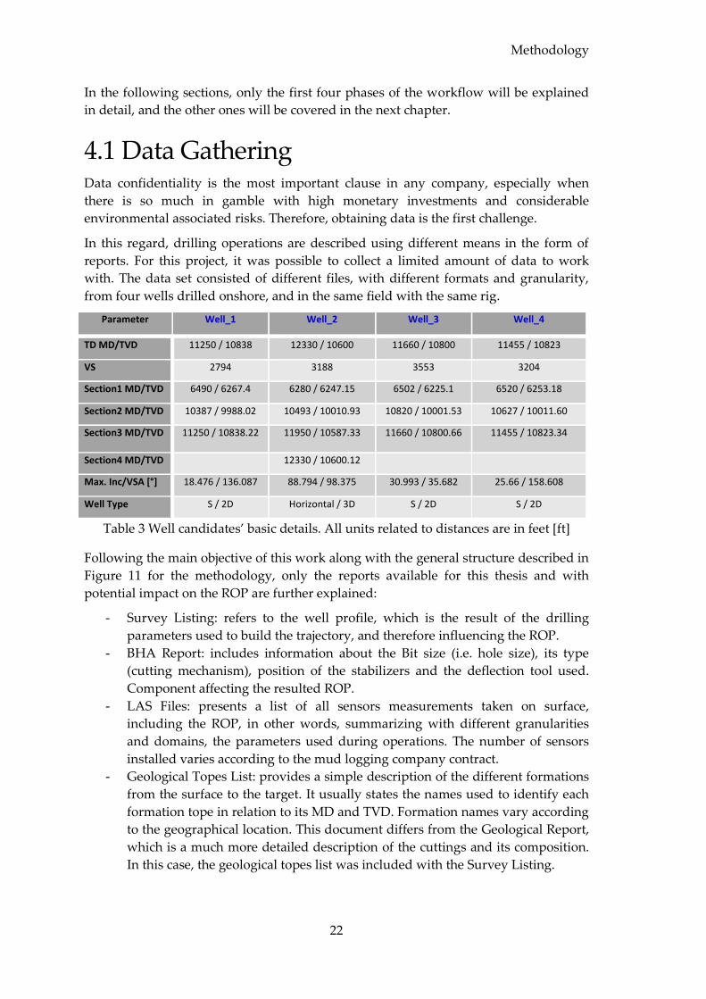
reports. For this project, it was possible to collect a limited amount of data to work
with. The data set consisted of different files, with different formats and granularity,
from four wells drilled onshore, and in the same field with the same rig.
Parameter Well_1 Well_2 Well_3 Well_4
TD MD/TVD 11250 / 10838 12330 / 10600 11660 / 10800 11455 / 10823
VS 2794 3188 3553 3204
Section1 MD/TVD 6490 / 6267.4 6280 / 6247.15 6502 / 6225.1 6520 / 6253.18
Section2 MD/TVD 10387 / 9988.02 10493 / 10010.93 10820 / 10001.53 10627 / 10011.60
Section3 MD/TVD 11250 / 10838.22 11950 / 10587.33 11660 / 10800.66 11455 / 10823.34
Section4 MD/TVD 12330 / 10600.12
Max. Inc/VSA [°] 18.476 / 136.087 88.794 / 98.375 30.993 / 35.682 25.66 / 158.608
Well Type S / 2D Horizontal / 3D S / 2D S / 2D
Table 3 Well candidates’ basic details. All units related to distances are in feet [ft]
Following the main objective of this work along with the general structure described in
Figure 11 for the methodology, only the reports available for this thesis and with
potential impact on the ROP are further explained:
- Survey Listing: refers to the well profile, which is the result of the drilling
parameters used to build the trajectory, and therefore influencing the ROP.
- BHA Report: includes information about the Bit size (i.e. hole size), its type
(cutting mechanism), position of the stabilizers and the deflection tool used.
Component affecting the resulted ROP.
- LAS Files: presents a list of all sensors measurements taken on surface,
including the ROP, in other words, summarizing with different granularities
and domains, the parameters used during operations. The number of sensors
installed varies according to the mud logging company contract.
- Geological Topes List: provides a simple description of the different formations
from the surface to the target. It usually states the names used to identify each
formation tope in relation to its MD and TVD. Formation names vary according
to the geographical location. This document differs from the Geological Report,
which is a much more detailed description of the cuttings and its composition.
In this case, the geological topes list was included with the Survey Listing.
Methodology
23
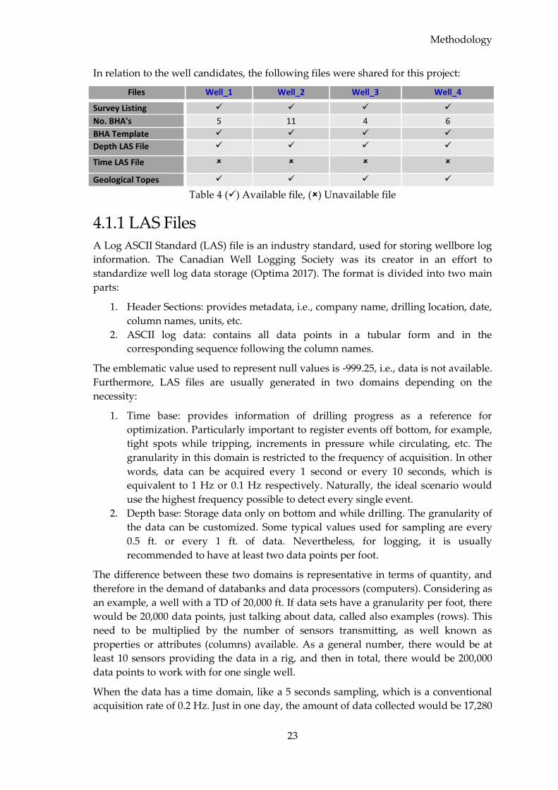
In relation to the well candidates, the following files were shared for this project:
Files Well_1 Well_2 Well_3 Well_4
Survey Listing
No. BHA's 5 11 4 6
BHA Template
Depth LAS File
Time LAS File
Geological Topes
Table 4 () Available file, () Unavailable file
4.1.1 LAS Files A Log ASCII Standard (LAS) file is an industry standard, used for storing wellbore log
information. The Canadian Well Logging Society was its creator in an effort to
standardize well log data storage (Optima 2017). The format is divided into two main
parts:
1. Header Sections: provides metadata, i.e., company name, drilling location, date,
column names, units, etc.
2. ASCII log data: contains all data points in a tubular form and in the
corresponding sequence following the column names.
The emblematic value used to represent null values is -999.25, i.e., data is not available.
Furthermore, LAS files are usually generated in two domains depending on the
necessity:
1. Time base: provides information of drilling progress as a reference for
optimization. Particularly important to register events off bottom, for example,
tight spots while tripping, increments in pressure while circulating, etc. The
granularity in this domain is restricted to the frequency of acquisition. In other
words, data can be acquired every 1 second or every 10 seconds, which is
equivalent to 1 Hz or 0.1 Hz respectively. Naturally, the ideal scenario would
use the highest frequency possible to detect every single event.
2. Depth base: Storage data only on bottom and while drilling. The granularity of
the data can be customized. Some typical values used for sampling are every
0.5 ft. or every 1 ft. of data. Nevertheless, for logging, it is usually
recommended to have at least two data points per foot.
The difference between these two domains is representative in terms of quantity, and
therefore in the demand of databanks and data processors (computers). Considering as
an example, a well with a TD of 20,000 ft. If data sets have a granularity per foot, there
would be 20,000 data points, just talking about data, called also examples (rows). This
need to be multiplied by the number of sensors transmitting, as well known as
properties or attributes (columns) available. As a general number, there would be at
least 10 sensors providing the data in a rig, and then in total, there would be 200,000
data points to work with for one single well.
When the data has a time domain, like a 5 seconds sampling, which is a conventional
acquisition rate of 0.2 Hz. Just in one day, the amount of data collected would be 17,280
Methodology
24
data points for one single property. Like in the previous example, assuming 10
measurements, the amount of data for one day would be 172,800 examples. Then the
duration of a well needs to be included in the final calculation and using a conservative
value of 15 days, the final amount of data per well would be approximately 2’592,000
data points. To sum up, when the file domain is time, data points are roughly
estimated as 10 times higher than when using a depth domain.
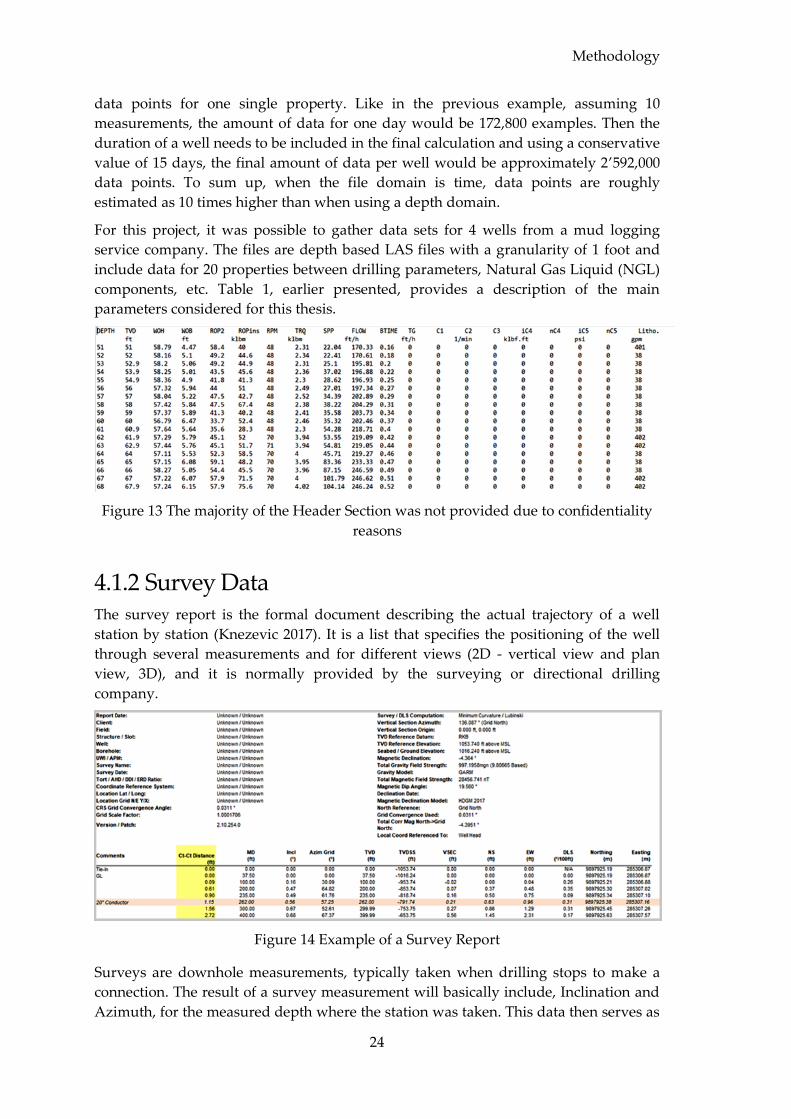
For this project, it was possible to gather data sets for 4 wells from a mud logging
service company. The files are depth based LAS files with a granularity of 1 foot and
include data for 20 properties between drilling parameters, Natural Gas Liquid (NGL)
components, etc. Table 1, earlier presented, provides a description of the main
parameters considered for this thesis.
Figure 13 The majority of the Header Section was not provided due to confidentiality
reasons
4.1.2 Survey Data The survey report is the formal document describing the actual trajectory of a well
station by station (Knezevic 2017). It is a list that specifies the positioning of the well
through several measurements and for different views (2D - vertical view and plan
view, 3D), and it is normally provided by the surveying or directional drilling
company.
Figure 14 Example of a Survey Report
Surveys are downhole measurements, typically taken when drilling stops to make a
connection. The result of a survey measurement will basically include, Inclination and
Azimuth, for the measured depth where the station was taken. This data then serves as
Methodology
25
input to calculate additional properties relevant for trajectory construction. Table 2,
presented in chapter 3, provides a brief description for the parameters considered in
this work. The format of a Survey Report might vary from client to client, but it usually
includes at least those three measurements. For this assignment, the survey reports for
the candidate wells included the geological tops information along with the casing
points’ depths.
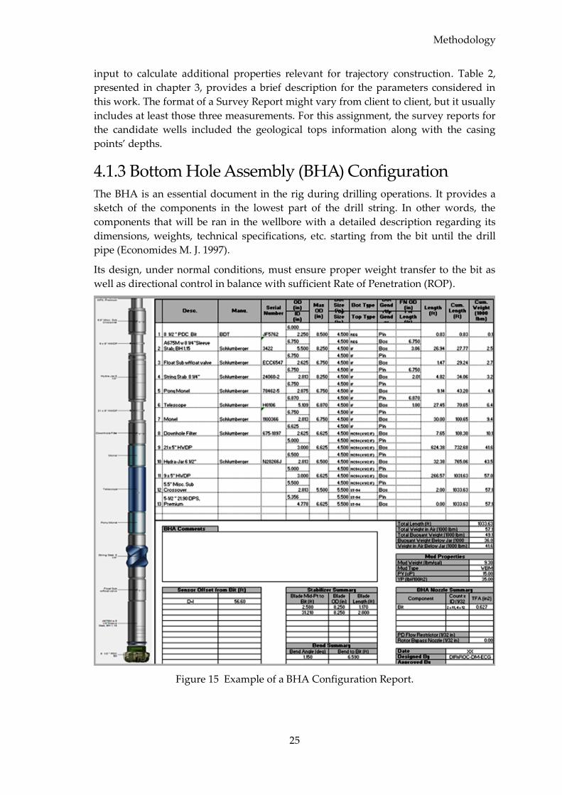
4.1.3 Bottom Hole Assembly (BHA) Configuration The BHA is an essential document in the rig during drilling operations. It provides a
sketch of the components in the lowest part of the drill string. In other words, the
components that will be ran in the wellbore with a detailed description regarding its
dimensions, weights, technical specifications, etc. starting from the bit until the drill
pipe (Economides M. J. 1997).
Its design, under normal conditions, must ensure proper weight transfer to the bit as
well as directional control in balance with sufficient Rate of Penetration (ROP).
Figure 15 Example of a BHA Configuration Report.
Methodology
26
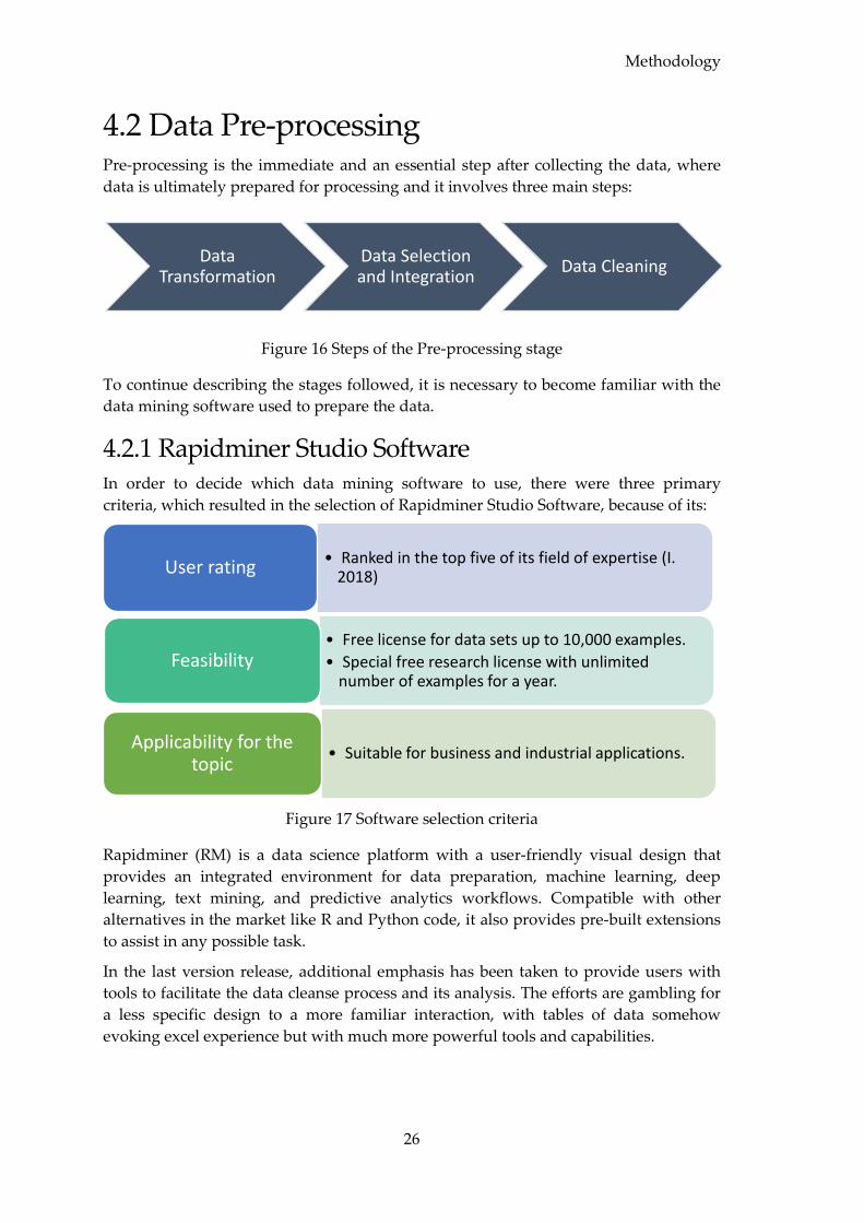
4.2 Data Pre-processing Pre-processing is the immediate and an essential step after collecting the data, where
data is ultimately prepared for processing and it involves three main steps:
Figure 16 Steps of the Pre-processing stage
To continue describing the stages followed, it is necessary to become familiar with the
data mining software used to prepare the data.
4.2.1 Rapidminer Studio Software In order to decide which data mining software to use, there were three primary
criteria, which resulted in the selection of Rapidminer Studio Software, because of its:
Figure 17 Software selection criteria
Rapidminer (RM) is a data science platform with a user-friendly visual design that
provides an integrated environment for data preparation, machine learning, deep
learning, text mining, and predictive analytics workflows. Compatible with other
alternatives in the market like R and Python code, it also provides pre-built extensions
to assist in any possible task.
In the last version release, additional emphasis has been taken to provide users with
tools to facilitate the data cleanse process and its analysis. The efforts are gambling for
a less specific design to a more familiar interaction, with tables of data somehow
evoking excel experience but with much more powerful tools and capabilities.
Data Transformation
Data Selection and Integration
Data Cleaning
• Ranked in the top five of its field of expertise (I. 2018)
User rating
• Free license for data sets up to 10,000 examples.
• Special free research license with unlimited number of examples for a year.
Feasibility
• Suitable for business and industrial applications.Applicability for the
topic
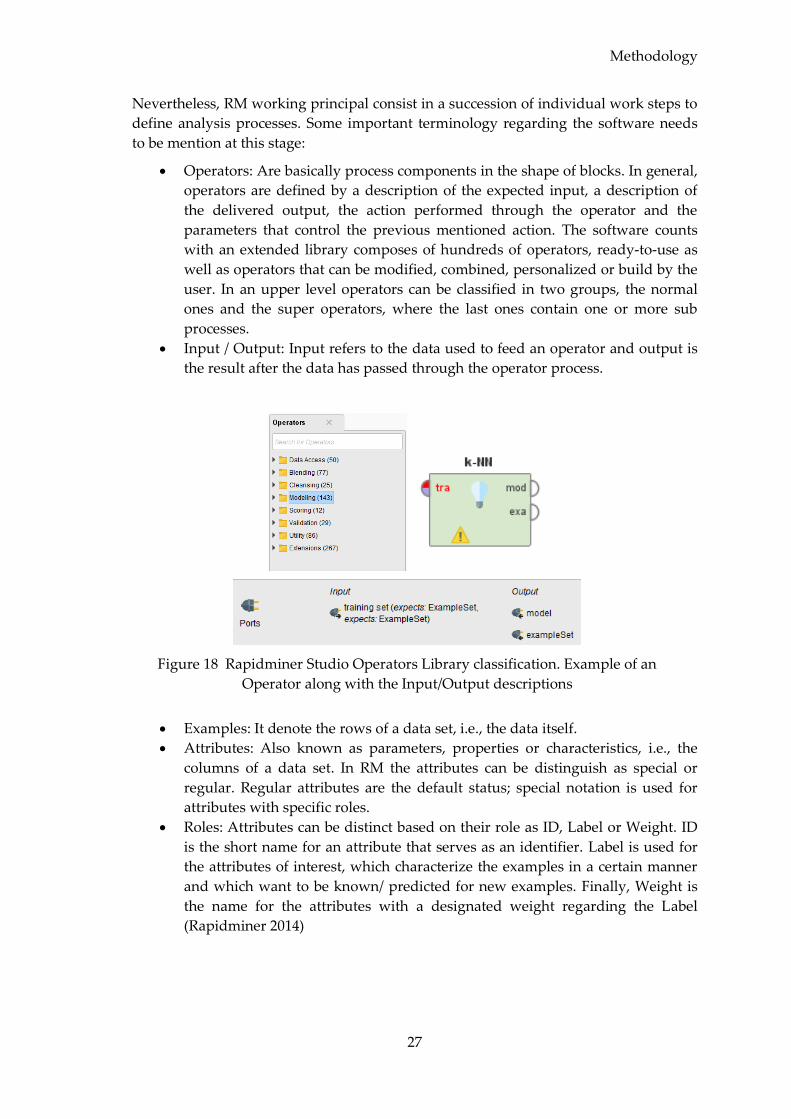
Methodology
27
Nevertheless, RM working principal consist in a succession of individual work steps to
define analysis processes. Some important terminology regarding the software needs
to be mention at this stage:
Operators: Are basically process components in the shape of blocks. In general,
operators are defined by a description of the expected input, a description of
the delivered output, the action performed through the operator and the
parameters that control the previous mentioned action. The software counts
with an extended library composes of hundreds of operators, ready-to-use as
well as operators that can be modified, combined, personalized or build by the
user. In an upper level operators can be classified in two groups, the normal
ones and the super operators, where the last ones contain one or more sub
processes.
Input / Output: Input refers to the data used to feed an operator and output is
the result after the data has passed through the operator process.
Figure 18 Rapidminer Studio Operators Library classification. Example of an
Operator along with the Input/Output descriptions
Examples: It denote the rows of a data set, i.e., the data itself.
Attributes: Also known as parameters, properties or characteristics, i.e., the
columns of a data set. In RM the attributes can be distinguish as special or
regular. Regular attributes are the default status; special notation is used for
attributes with specific roles.
Roles: Attributes can be distinct based on their role as ID, Label or Weight. ID
is the short name for an attribute that serves as an identifier. Label is used for
the attributes of interest, which characterize the examples in a certain manner
and which want to be known/ predicted for new examples. Finally, Weight is
the name for the attributes with a designated weight regarding the Label
(Rapidminer 2014)

Methodology
28
Figure 19 Data view through Examples, regular and special attributes
Data type: also known as Value Type, because it is an indication of the value of
the attribute. There are different value types, and they can also be transformed
into other type when necessary. Still, the main groups are text in the case of
free text, numerical when numbers are involved and nominal when only few
values are possible (Rapidminer 2014). Regarding this work, the following
table summarize the values types used and automatically selected by RM when
reading the data:
Integer A positive or negative number which no fractional part.
Real A number that represent any quantity along a number line. Can be positive or
negative. (Page 2011)
Polynominal Special case of nominal type. Attributes can have more than two different
non-numerical values.
Table 5 Summarize of the value types used in the data sets.
With a general overview of the software chosen, it is important to mention that
basically all the data analysis and simulations were done using it. Nevertheless, part of
the data preparation was done using Excel in combination with Visual Basic Script
(VBS) and can be reviewed in detail in the Appendix A.1.
4.2.2 Data Transformation As previously described, two files are the main source of data: the depth based LAS
files and the survey listings. It is necessary to consider that both files have different
granularities; the LAS files provide data every 1 foot while the survey report provide
data at different fixed depths. In addition, the BHA Reports are per drilling run.
To follow the proposed methodology and asses the functionality of data mining, all
data must be imported in the RM software and be comparable too. The LAS files are
already with the appropriate base, but the survey listing demands additional attention
as well as the BHA reports, which need to be transform to the same base.
As the Survey Report is commonly exported in Excel, it was decided to use VBS to
develop a tool to make the calculation and the coding process automatically, based on
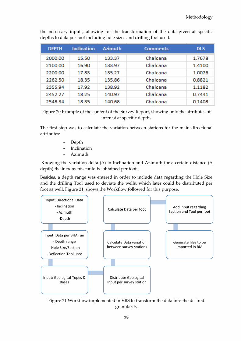
Methodology
29
the necessary inputs, allowing for the transformation of the data given at specific
depths to data per foot including hole sizes and drilling tool used.
Figure 20 Example of the content of the Survey Report, showing only the attributes of
interest at specific depths
The first step was to calculate the variation between stations for the main directional
attributes:
- Depth
- Inclination
- Azimuth
Knowing the variation delta (Δ) in Inclination and Azimuth for a certain distance (Δ
depth) the increments could be obtained per foot.
Besides, a depth range was entered in order to include data regarding the Hole Size
and the drilling Tool used to deviate the wells, which later could be distributed per
foot as well. Figure 21, shows the Workflow followed for this purpose.
Figure 21 Workflow implemented in VBS to transform the data into the desired
granularity
Input: Directional Data
- Inclination
- Azimuth
-Depth
Input: Data per BHA run
- Depth range
- Hole Size/Section
- Deflection Tool used
Input: Geological Topes & Bases
Distribute Geological Input per survey station
Calculate Data variation between survey stations
Calculate Data per footAdd Input regarding
Section and Tool per foot
Generate files to be imported in RM

Methodology
30
The result is showed in Directional and Geological Data per foot.Figure 22 providing
Directional Data, Geological topes, Hole Size and Drilling Tool used per foot.
Furthermore, other directional attributes were calculated as well:
- Dogleg Severity (DLS): It is a measure of the amount of change in the
inclination and azimuth of a borehole, expressed in degrees per 100 feet
or per 30 meters course length. It’s calculation is based on the Minimum
Curvature Method as it is the standard method used in the Industry
(Asad 2016).
𝐷𝐿𝑆 =100
𝑑𝑠𝑐𝑜𝑠−1{𝑠𝑖𝑛𝐼1𝑠𝑖𝑛𝐼2 cos(𝐴2 − 𝐴1) + 𝑐𝑜𝑠𝐼1𝑐𝑜𝑠𝐼2}
(1)
Where ds is the course length between survey stations 1 and 2
I1, I2 are the Inclinations in survey stations respectively
A1, A2 are the Azimuths in survey stations respectively.
- Build-rate angle (BR): refers to the increase or decrease in Inclination
from vertical per 100 ft. or 30 m.
𝐵𝑅 = 𝑑𝐼(𝑠)
𝑑𝑠= ∆𝐼
(2)
- Turn-rate angle (TR): is the degree of change in the Azimuth per 100 ft.
or 30 m.
𝑇𝑅 = 𝑑𝐴(𝑠)
𝑑𝑠= ∆𝐴
(3)
Figure 22 Directional and Geological Data per foot.
4.2.3 Project creation and Data Loading With the files ready to be imported into RM, it was necessary to create the project and
get familiar with the kind of operators suitable for the task. Appendix A.2 contains a
list of the main operators used to create the different processes which are also detailed
in the Appendix A.3. During the following steps, all RM processes will be referenced
by their process’ names in parenthesis for its further reference in the mentioned
appendix.
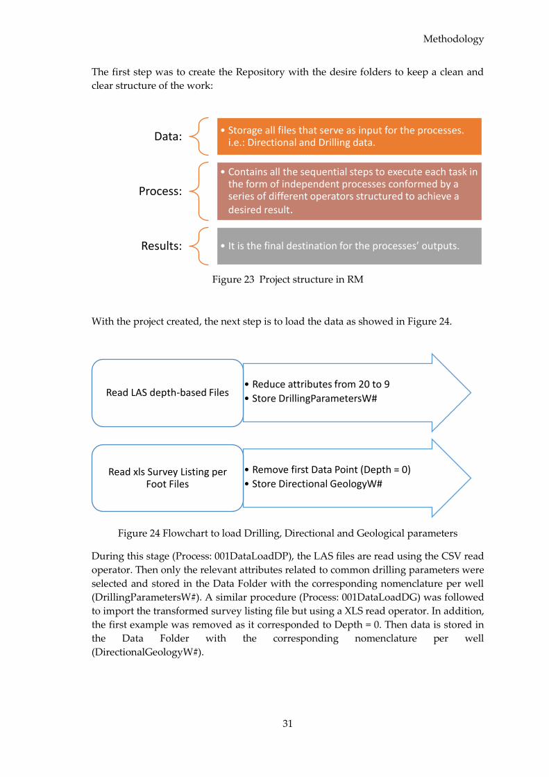
Methodology
31
The first step was to create the Repository with the desire folders to keep a clean and
clear structure of the work:
Figure 23 Project structure in RM
With the project created, the next step is to load the data as showed in Figure 24.
Figure 24 Flowchart to load Drilling, Directional and Geological parameters
During this stage (Process: 001DataLoadDP), the LAS files are read using the CSV read
operator. Then only the relevant attributes related to common drilling parameters were
selected and stored in the Data Folder with the corresponding nomenclature per well
(DrillingParametersW#). A similar procedure (Process: 001DataLoadDG) was followed
to import the transformed survey listing file but using a XLS read operator. In addition,
the first example was removed as it corresponded to Depth = 0. Then data is stored in
the Data Folder with the corresponding nomenclature per well
(DirectionalGeologyW#).
Data:• Storage all files that serve as input for the processes.
i.e.: Directional and Drilling data.
Process:
• Contains all the sequential steps to execute each task in the form of independent processes conformed by a series of different operators structured to achieve a desired result.
Results: • It is the final destination for the processes’ outputs.
• Reduce attributes from 20 to 9
• Store DrillingParametersW#Read LAS depth-based Files
• Remove first Data Point (Depth = 0)
• Store Directional GeologyW#Read xls Survey Listing per
Foot Files
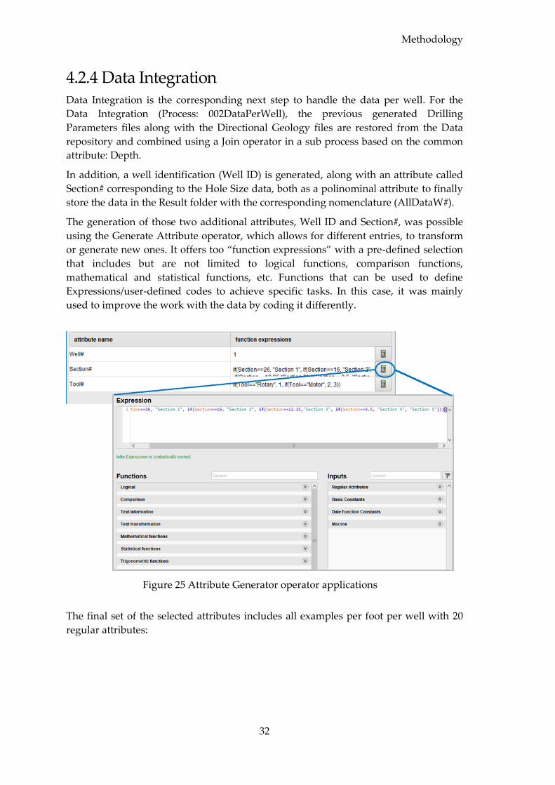
Methodology
32
4.2.4 Data Integration Data Integration is the corresponding next step to handle the data per well. For the
Data Integration (Process: 002DataPerWell), the previous generated Drilling
Parameters files along with the Directional Geology files are restored from the Data
repository and combined using a Join operator in a sub process based on the common
attribute: Depth.
In addition, a well identification (Well ID) is generated, along with an attribute called
Section# corresponding to the Hole Size data, both as a polinominal attribute to finally
store the data in the Result folder with the corresponding nomenclature (AllDataW#).
The generation of those two additional attributes, Well ID and Section#, was possible
using the Generate Attribute operator, which allows for different entries, to transform
or generate new ones. It offers too “function expressions” with a pre-defined selection
that includes but are not limited to logical functions, comparison functions,
mathematical and statistical functions, etc. Functions that can be used to define
Expressions/user-defined codes to achieve specific tasks. In this case, it was mainly
used to improve the work with the data by coding it differently.
Figure 25 Attribute Generator operator applications
The final set of the selected attributes includes all examples per foot per well with 20
regular attributes:
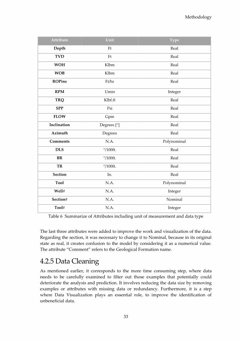
Methodology
33
Attribute Unit Type
Depth Ft Real
TVD Ft Real
WOH Klbm Real
WOB Klbm Real
ROPins Ft/hr Real
RPM 1/min Integer
TRQ Klbf.ft Real
SPP Psi Real
FLOW Gpm Real
Inclination Degrees [°] Real
Azimuth Degrees Real
Comments N.A. Polynominal
DLS °/100ft. Real
BR °/100ft. Real
TR °/100ft. Real
Section In. Real
Tool N.A. Polynominal
Well# N.A. Integer
Section# N.A. Nominal
Tool# N.A. Integer
Table 6 Summarize of Attributes including unit of measurement and data type
The last three attributes were added to improve the work and visualization of the data.
Regarding the section, it was necessary to change it to Nominal, because in its original
state as real, it creates confusion to the model by considering it as a numerical value.
The attribute “Comment” refers to the Geological Formation name.
4.2.5 Data Cleaning As mentioned earlier, it corresponds to the more time consuming step, where data
needs to be carefully examined to filter out those examples that potentially could
deteriorate the analysis and prediction. It involves reducing the data size by removing
examples or attributes with missing data or redundancy. Furthermore, it is a step
where Data Visualization plays an essential role, to improve the identification of
unbeneficial data.
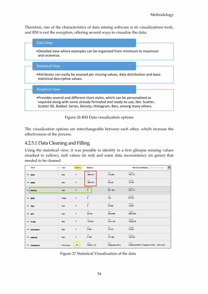
Methodology
34
Therefore, one of the characteristics of data mining software is its visualizations tools,
and RM is not the exception, offering several ways to visualize the data:
Figure 26 RM Data visualization options
The visualization options are interchangeable between each other, which increase the
effectiveness of the process.
4.2.5.1 Data Cleaning and Filling
Using the statistical view, it was possible to identify in a first glimpse missing values
(marked in yellow), null values (in red) and some data inconsistency (in green) that
needed to be cleaned.
Figure 27 Statistical Visualization of the data
•Detailed view where examples can be organized from minimum to maximum and viceversa.
Data View
•Attributes can easily be assesed per missing values, data distribution and basic statistical descriptive values.
Statistical View
•Provides several and different chart styles, which can be personalized as required along with some already formated and ready-to-use, like: Scatter, Scatter 3D, Bubbel, Series, Density, Histogram, Bars, among many others.
Graphical View
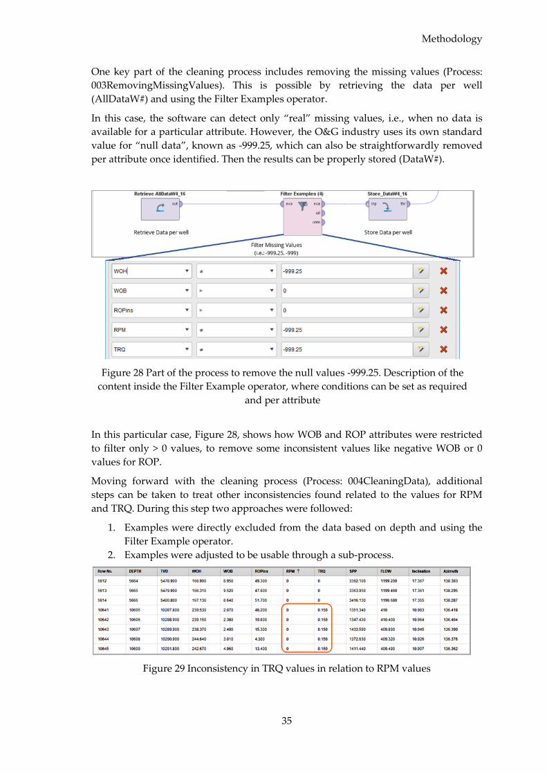
Methodology
35
One key part of the cleaning process includes removing the missing values (Process:
003RemovingMissingValues). This is possible by retrieving the data per well
(AllDataW#) and using the Filter Examples operator.
In this case, the software can detect only “real” missing values, i.e., when no data is
available for a particular attribute. However, the O&G industry uses its own standard
value for “null data”, known as -999.25, which can also be straightforwardly removed
per attribute once identified. Then the results can be properly stored (DataW#).
Figure 28 Part of the process to remove the null values -999.25. Description of the
content inside the Filter Example operator, where conditions can be set as required
and per attribute
In this particular case, Figure 28, shows how WOB and ROP attributes were restricted
to filter only > 0 values, to remove some inconsistent values like negative WOB or 0
values for ROP.
Moving forward with the cleaning process (Process: 004CleaningData), additional
steps can be taken to treat other inconsistencies found related to the values for RPM
and TRQ. During this step two approaches were followed:
1. Examples were directly excluded from the data based on depth and using the
Filter Example operator.
2. Examples were adjusted to be usable through a sub-process.
Figure 29 Inconsistency in TRQ values in relation to RPM values
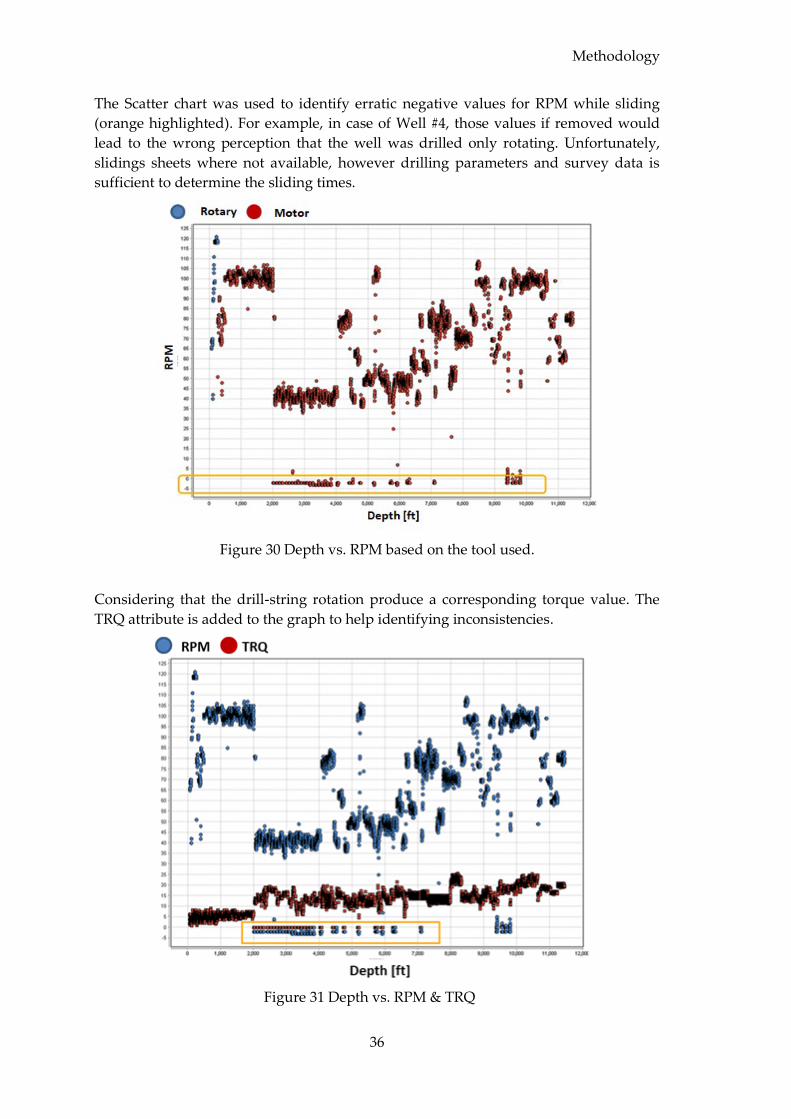
Methodology
36
The Scatter chart was used to identify erratic negative values for RPM while sliding
(orange highlighted). For example, in case of Well #4, those values if removed would
lead to the wrong perception that the well was drilled only rotating. Unfortunately,
slidings sheets where not available, however drilling parameters and survey data is
sufficient to determine the sliding times.
Figure 30 Depth vs. RPM based on the tool used.
Considering that the drill-string rotation produce a corresponding torque value. The
TRQ attribute is added to the graph to help identifying inconsistencies.
Figure 31 Depth vs. RPM & TRQ
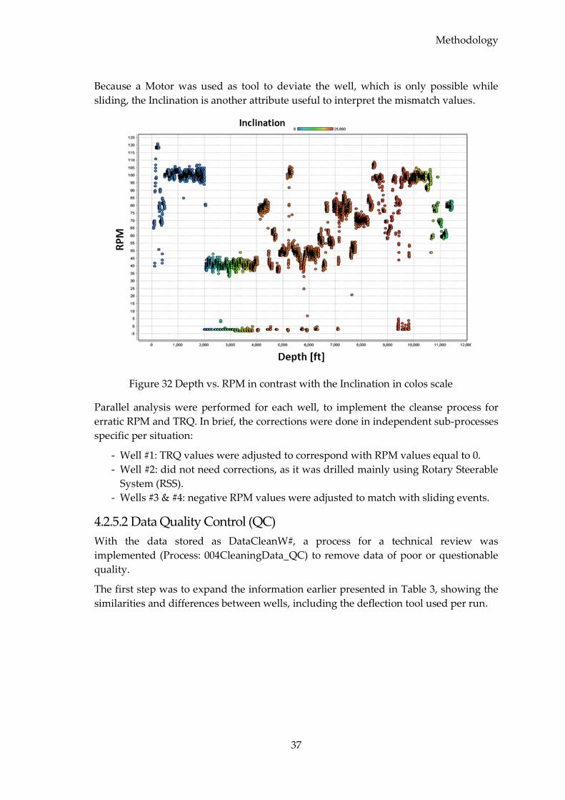
Methodology
37
Because a Motor was used as tool to deviate the well, which is only possible while
sliding, the Inclination is another attribute useful to interpret the mismatch values.
Figure 32 Depth vs. RPM in contrast with the Inclination in colos scale
Parallel analysis were performed for each well, to implement the cleanse process for
erratic RPM and TRQ. In brief, the corrections were done in independent sub-processes
specific per situation:
- Well #1: TRQ values were adjusted to correspond with RPM values equal to 0.
- Well #2: did not need corrections, as it was drilled mainly using Rotary Steerable
System (RSS).
- Wells #3 & #4: negative RPM values were adjusted to match with sliding events.
4.2.5.2 Data Quality Control (QC)
With the data stored as DataCleanW#, a process for a technical review was
implemented (Process: 004CleaningData_QC) to remove data of poor or questionable
quality.
The first step was to expand the information earlier presented in Table 3, showing the
similarities and differences between wells, including the deflection tool used per run.
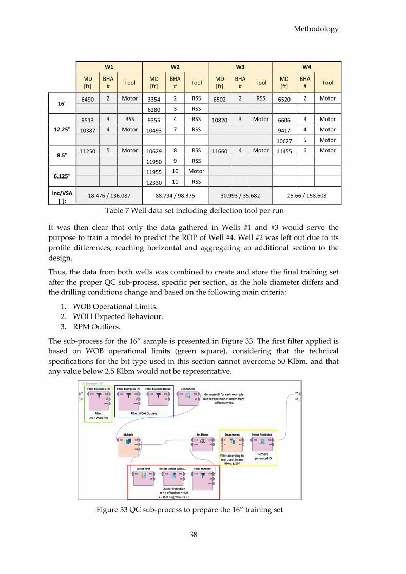
Methodology
38
W1 W2 W3 W4
MD [ft]
BHA #
Tool MD [ft]
BHA #
Tool MD [ft]
BHA #
Tool MD [ft]
BHA #
Tool
16" 6490 2 Motor 3354 2 RSS 6502 2 RSS 6520 2 Motor
6280 3 RSS
12.25"
9513 3 RSS 9355 4 RSS 10820 3 Motor 6606 3 Motor
10387 4 Motor 10493 7 RSS 9417 4 Motor
10627 5 Motor
8.5" 11250 5 Motor 10629 8 RSS 11660 4 Motor 11455 6 Motor
11950 9 RSS
6.125" 11955 10 Motor
12330 11 RSS
Inc/VSA [°]:
18.476 / 136.087 88.794 / 98.375 30.993 / 35.682 25.66 / 158.608
Table 7 Well data set including deflection tool per run
It was then clear that only the data gathered in Wells #1 and #3 would serve the
purpose to train a model to predict the ROP of Well #4. Well #2 was left out due to its
profile differences, reaching horizontal and aggregating an additional section to the
design.
Thus, the data from both wells was combined to create and store the final training set
after the proper QC sub-process, specific per section, as the hole diameter differs and
the drilling conditions change and based on the following main criteria:
1. WOB Operational Limits.
2. WOH Expected Behaviour.
3. RPM Outliers.
The sub-process for the 16” sample is presented in Figure 33. The first filter applied is
based on WOB operational limits (green square), considering that the technical
specifications for the bit type used in this section cannot overcome 50 Klbm, and that
any value below 2.5 Klbm would not be representative.
Figure 33 QC sub-process to prepare the 16” training set
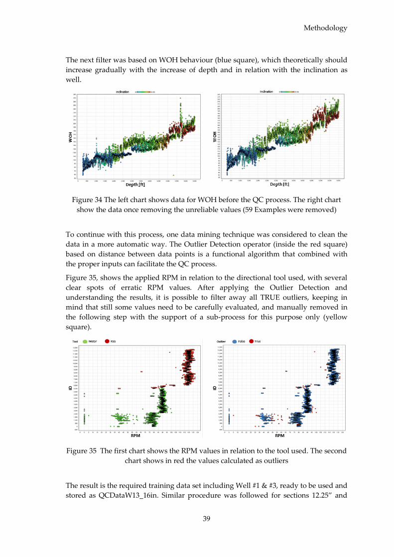
Methodology
39
The next filter was based on WOH behaviour (blue square), which theoretically should
increase gradually with the increase of depth and in relation with the inclination as
well.
Figure 34 The left chart shows data for WOH before the QC process. The right chart
show the data once removing the unreliable values (59 Examples were removed)
To continue with this process, one data mining technique was considered to clean the
data in a more automatic way. The Outlier Detection operator (inside the red square)
based on distance between data points is a functional algorithm that combined with
the proper inputs can facilitate the QC process.
Figure 35, shows the applied RPM in relation to the directional tool used, with several
clear spots of erratic RPM values. After applying the Outlier Detection and
understanding the results, it is possible to filter away all TRUE outliers, keeping in
mind that still some values need to be carefully evaluated, and manually removed in
the following step with the support of a sub-process for this purpose only (yellow
square).
Figure 35 The first chart shows the RPM values in relation to the tool used. The second
chart shows in red the values calculated as outliers
The result is the required training data set including Well #1 & #3, ready to be used and
stored as QCDataW13_16in. Similar procedure was followed for sections 12.25” and
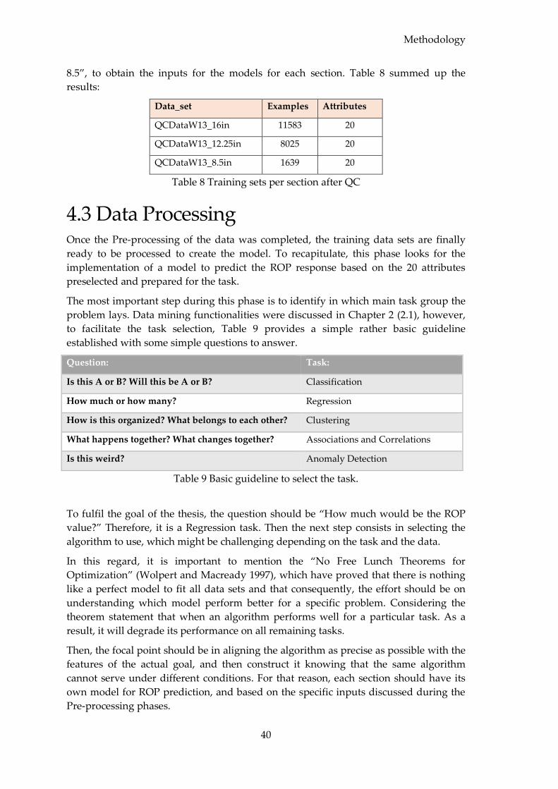
Methodology
40
8.5”, to obtain the inputs for the models for each section. Table 8 summed up the
results:
Data_set Examples Attributes
QCDataW13_16in 11583 20
QCDataW13_12.25in 8025 20
QCDataW13_8.5in 1639 20
Table 8 Training sets per section after QC
4.3 Data Processing Once the Pre-processing of the data was completed, the training data sets are finally
ready to be processed to create the model. To recapitulate, this phase looks for the
implementation of a model to predict the ROP response based on the 20 attributes
preselected and prepared for the task.
The most important step during this phase is to identify in which main task group the
problem lays. Data mining functionalities were discussed in Chapter 2 (2.1), however,
to facilitate the task selection, Table 9 provides a simple rather basic guideline
established with some simple questions to answer.
Question: Task:
Is this A or B? Will this be A or B? Classification
How much or how many? Regression
How is this organized? What belongs to each other? Clustering
What happens together? What changes together? Associations and Correlations
Is this weird? Anomaly Detection
Table 9 Basic guideline to select the task.
To fulfil the goal of the thesis, the question should be “How much would be the ROP
value?” Therefore, it is a Regression task. Then the next step consists in selecting the
algorithm to use, which might be challenging depending on the task and the data.
In this regard, it is important to mention the “No Free Lunch Theorems for
Optimization” (Wolpert and Macready 1997), which have proved that there is nothing
like a perfect model to fit all data sets and that consequently, the effort should be on
understanding which model perform better for a specific problem. Considering the
theorem statement that when an algorithm performs well for a particular task. As a
result, it will degrade its performance on all remaining tasks.
Then, the focal point should be in aligning the algorithm as precise as possible with the
features of the actual goal, and then construct it knowing that the same algorithm
cannot serve under different conditions. For that reason, each section should have its
own model for ROP prediction, and based on the specific inputs discussed during the
Pre-processing phases.
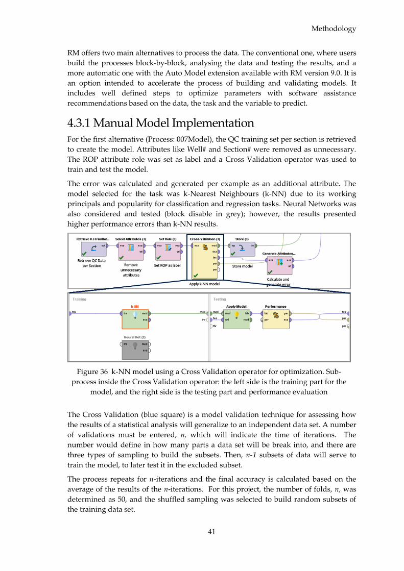
Methodology
41
RM offers two main alternatives to process the data. The conventional one, where users
build the processes block-by-block, analysing the data and testing the results, and a
more automatic one with the Auto Model extension available with RM version 9.0. It is
an option intended to accelerate the process of building and validating models. It
includes well defined steps to optimize parameters with software assistance
recommendations based on the data, the task and the variable to predict.
4.3.1 Manual Model Implementation For the first alternative (Process: 007Model), the QC training set per section is retrieved
to create the model. Attributes like Well# and Section# were removed as unnecessary.
The ROP attribute role was set as label and a Cross Validation operator was used to
train and test the model.
The error was calculated and generated per example as an additional attribute. The
model selected for the task was k-Nearest Neighbours (k-NN) due to its working
principals and popularity for classification and regression tasks. Neural Networks was
also considered and tested (block disable in grey); however, the results presented
higher performance errors than k-NN results.
Figure 36 k-NN model using a Cross Validation operator for optimization. Sub-
process inside the Cross Validation operator: the left side is the training part for the
model, and the right side is the testing part and performance evaluation
The Cross Validation (blue square) is a model validation technique for assessing how
the results of a statistical analysis will generalize to an independent data set. A number
of validations must be entered, n, which will indicate the time of iterations. The
number would define in how many parts a data set will be break into, and there are
three types of sampling to build the subsets. Then, n-1 subsets of data will serve to
train the model, to later test it in the excluded subset.
The process repeats for n-iterations and the final accuracy is calculated based on the
average of the results of the n-iterations. For this project, the number of folds, n, was
determined as 50, and the shuffled sampling was selected to build random subsets of
the training data set.
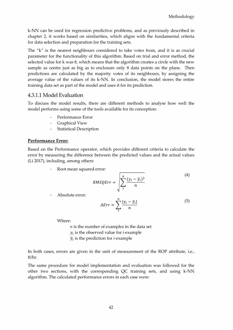
Methodology
42
k-NN can be used for regression predictive problems, and as previously described in
chapter 2, it works based on similarities, which aligns with the fundamental criteria
for data selection and preparation for the training sets.
The “k” is the nearest neighbours considered to take votes from, and it is as crucial
parameter for the functionality of this algorithm. Based on trial and error method, the
selected value for k was 8, which means that the algorithm creates a circle with the new
sample as centre just as big as to enclosure only 8 data points on the plane. Then
predictions are calculated by the majority votes of its neighbours, by assigning the
average value of the values of its k-NN. In conclusion, the model stores the entire
training data set as part of the model and uses it for its prediction.
4.3.1.1 Model Evaluation
To discuss the model results, there are different methods to analyse how well the
model performs using some of the tools available for its conception:
- Performance Error
- Graphical View
- Statistical Description
Performance Error:
Based on the Performance operator, which provides different criteria to calculate the
error by measuring the difference between the predicted values and the actual values
(Li 2017), including, among others:
- Root mean squared error:
𝑅𝑀𝑆𝑄𝐸𝑟𝑟 = √∑(𝑦𝑖 − �̅�𝑖)2
𝑛
𝑛
1
(4)
- Absolute error:
𝐴𝐸𝑟𝑟 = ∑|𝑦𝑖 − �̅�𝑖|
𝑛
𝑛
1
(5)
Where:
n is the number of examples in the data set
𝑦𝑖 is the observed value for i-example
�̅�𝑖 is the prediction for i-example
In both cases, errors are given in the unit of measurement of the ROP attribute, i.e.,
ft/hr.
The same procedure for model implementation and evaluation was followed for the
other two sections, with the corresponding QC training sets, and using k-NN
algorithm. The calculated performance errors in each case were:
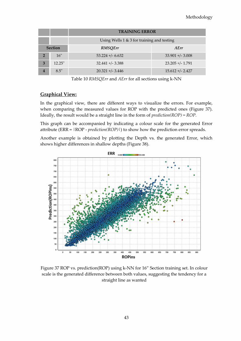
Methodology
43
TRAINING ERROR
Using Wells 1 & 3 for training and testing
Section RMSQErr AErr
2 16" 53.224 +/- 6.632 33.901 +/- 3.008
3 12.25" 32.441 +/- 3.388 23.205 +/- 1.791
4 8.5" 20.321 +/- 3.446 15.612 +/- 2.427
Table 10 RMSQErr and AErr for all sections using k-NN
Graphical View:
In the graphical view, there are different ways to visualize the errors. For example,
when comparing the measured values for ROP with the predicted ones (Figure 37).
Ideally, the result would be a straight line in the form of prediction(ROP) = ROP.
This graph can be accompanied by indicating a colour scale for the generated Error
attribute (ERR = |ROP - prediction(ROP)|) to show how the prediction error spreads.
Another example is obtained by plotting the Depth vs. the generated Error, which
shows higher differences in shallow depths (Figure 38).
Figure 37 ROP vs. prediction(ROP) using k-NN for 16” Section training set. In colour
scale is the generated difference between both values, suggesting the tendency for a
straight line as wanted
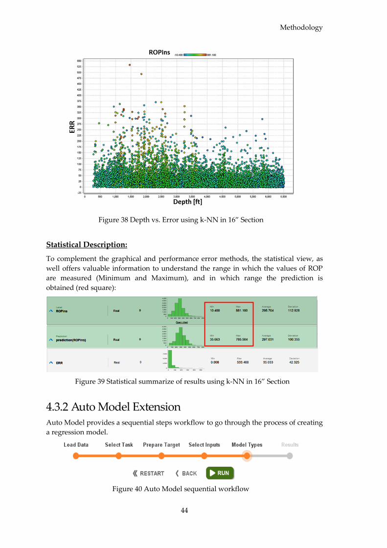
Methodology
44
Figure 38 Depth vs. Error using k-NN in 16” Section
Statistical Description:
To complement the graphical and performance error methods, the statistical view, as
well offers valuable information to understand the range in which the values of ROP
are measured (Minimum and Maximum), and in which range the prediction is
obtained (red square):
Figure 39 Statistical summarize of results using k-NN in 16” Section
4.3.2 Auto Model Extension Auto Model provides a sequential steps workflow to go through the process of creating
a regression model.
Figure 40 Auto Model sequential workflow
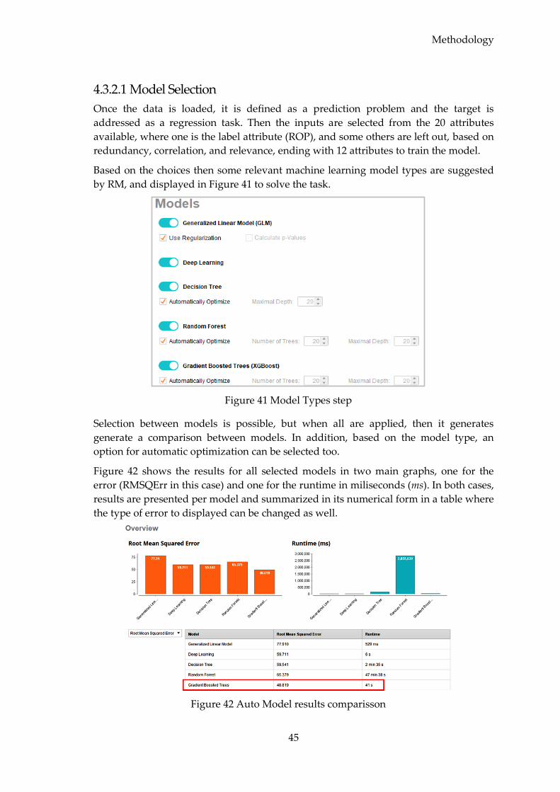
Methodology
45
4.3.2.1 Model Selection
Once the data is loaded, it is defined as a prediction problem and the target is
addressed as a regression task. Then the inputs are selected from the 20 attributes
available, where one is the label attribute (ROP), and some others are left out, based on
redundancy, correlation, and relevance, ending with 12 attributes to train the model.
Based on the choices then some relevant machine learning model types are suggested
by RM, and displayed in Figure 41 to solve the task.
Figure 41 Model Types step
Selection between models is possible, but when all are applied, then it generates
generate a comparison between models. In addition, based on the model type, an
option for automatic optimization can be selected too.
Figure 42 shows the results for all selected models in two main graphs, one for the
error (RMSQErr in this case) and one for the runtime in miliseconds (ms). In both cases,
results are presented per model and summarized in its numerical form in a table where
the type of error to displayed can be changed as well.
Figure 42 Auto Model results comparisson
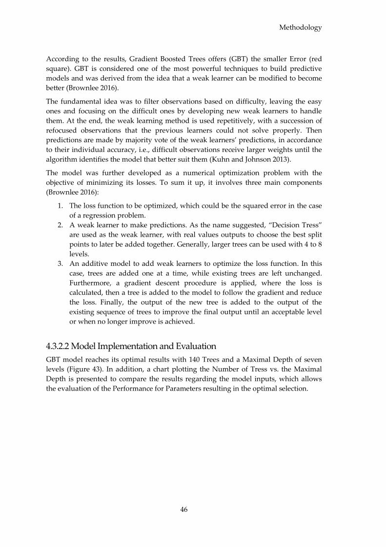
Methodology
46
According to the results, Gradient Boosted Trees offers (GBT) the smaller Error (red
square). GBT is considered one of the most powerful techniques to build predictive
models and was derived from the idea that a weak learner can be modified to become
better (Brownlee 2016).
The fundamental idea was to filter observations based on difficulty, leaving the easy
ones and focusing on the difficult ones by developing new weak learners to handle
them. At the end, the weak learning method is used repetitively, with a succession of
refocused observations that the previous learners could not solve properly. Then
predictions are made by majority vote of the weak learners’ predictions, in accordance
to their individual accuracy, i.e., difficult observations receive larger weights until the
algorithm identifies the model that better suit them (Kuhn and Johnson 2013).
The model was further developed as a numerical optimization problem with the
objective of minimizing its losses. To sum it up, it involves three main components
(Brownlee 2016):
1. The loss function to be optimized, which could be the squared error in the case
of a regression problem.
2. A weak learner to make predictions. As the name suggested, “Decision Tress”
are used as the weak learner, with real values outputs to choose the best split
points to later be added together. Generally, larger trees can be used with 4 to 8
levels.
3. An additive model to add weak learners to optimize the loss function. In this
case, trees are added one at a time, while existing trees are left unchanged.
Furthermore, a gradient descent procedure is applied, where the loss is
calculated, then a tree is added to the model to follow the gradient and reduce
the loss. Finally, the output of the new tree is added to the output of the
existing sequence of trees to improve the final output until an acceptable level
or when no longer improve is achieved.
4.3.2.2 Model Implementation and Evaluation
GBT model reaches its optimal results with 140 Trees and a Maximal Depth of seven
levels (Figure 43). In addition, a chart plotting the Number of Tress vs. the Maximal
Depth is presented to compare the results regarding the model inputs, which allows
the evaluation of the Performance for Parameters resulting in the optimal selection.
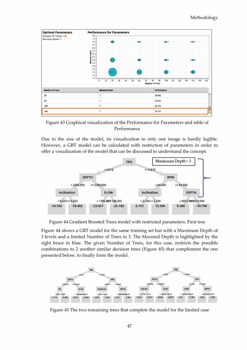
Methodology
47
Figure 43 Graphical visualization of the Performance for Parameters and table of
Performance
Due to the size of the model, its visualization in only one image is hardly legible.
However, a GBT model can be calculated with restriction of parameters in order to
offer a visualization of the model that can be discussed to understand the concept.
Figure 44 Gradient Boosted Trees model with restricted parameters. First tree
Figure 44 shows a GBT model for the same training set but with a Maximum Depth of
3 levels and a limited Number of Trees to 3. The Maximal Depth is highlighted by the
right brace in blue. The given Number of Trees, for this case, restricts the possible
combinations to 2 another similar decision trees (Figure 45) that complement the one
presented below, to finally form the model.
Figure 45 The two remaining trees that complete the model for the limited case
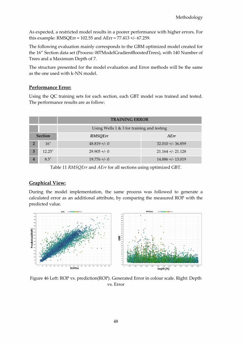
Methodology
48
As expected, a restricted model results in a poorer performance with higher errors. For
this example: RMSQErr = 102.55 and AErr = 77.413 +/- 67.259.
The following evaluation mainly corresponds to the GBM optimized model created for
the 16” Section data set (Process: 007ModelGradientBoostedTrees), with 140 Number of
Trees and a Maximum Depth of 7.
The structure presented for the model evaluation and Error methods will be the same
as the one used with k-NN model.
Performance Error:
Using the QC training sets for each section, each GBT model was trained and tested.
The performance results are as follow:
TRAINING ERROR
Using Wells 1 & 3 for training and testing
Section RMSQErr AErr
2 16" 48.819 +/- 0 32.010 +/- 36.859
3 12.25" 29.905 +/- 0 21.164 +/- 21.128
4 8.5" 19.776 +/- 0 14.886 +/- 13.019
Table 11 RMSQErr and AErr for all sections using optimized GBT.
Graphical View:
During the model implementation, the same process was followed to generate a
calculated error as an additional attribute, by comparing the measured ROP with the
predicted value.
Figure 46 Left: ROP vs. prediction(ROP). Generated Error in colour scale. Right: Depth
vs. Error
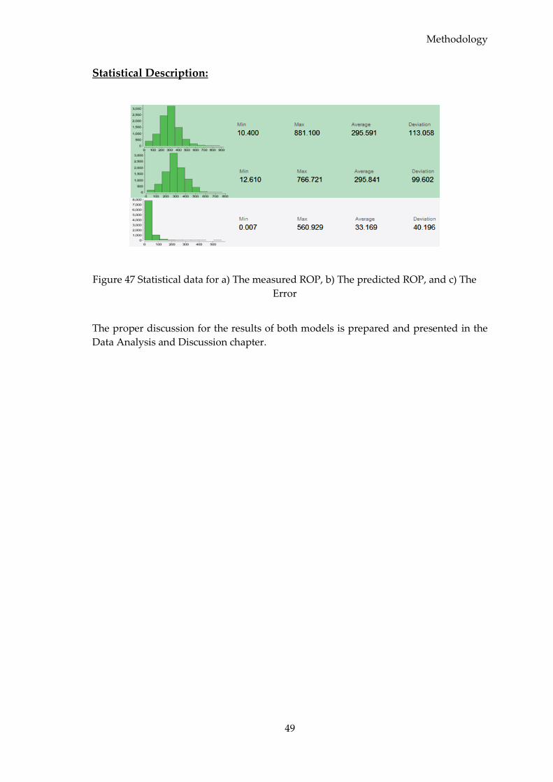
Methodology
49
Statistical Description:
Figure 47 Statistical data for a) The measured ROP, b) The predicted ROP, and c) The
Error
The proper discussion for the results of both models is prepared and presented in the
Data Analysis and Discussion chapter.

Methodology
50
Data Analysis and Results Discussion
51
Chapter 5 Data Analysis and Results
Discussion
With the data processed and prior to discuss the results, data needs to be further
analyzed using the visualization tools, considering the types of errors and using
descriptive statistics to improve the understanding of the variables on research.
5.1 Training Error and Prediction Error During the previous stage, models were implemented and tested, providing a
comparison between the measured values for ROP and the predicted ones. That
difference was called “Error”. However, in prediction modelling, there are two well-
defined types of errors, and quite different in importance (Nivre 2007):
1. Training error: Assess the model about the answer in comparison to the
training sample. The error is the mean error over the same data used for its
creation.
2. Prediction error: Also known as “Test error”, the model is tested with unseen
data sets. It refers on how well would do a model with an independent test
sample.
To this point, only the Training errors have been calculated and presented for the two
algorithms used, k-NN and GBT.
5.2 Model Evaluation In order to calculate the Prediction error, both models need to be tested in a “new”
Well. In this case, the initial data set included four Wells drilled in the same field and
in consequently order. Well #2 was excluded for the modelling due to its particularity
in the profile and design. Wells #1 and #3 were used to create the models, which can
now be tested in Well #4.
This stage is called deployment process (Process: 008Deployment), and its structure is
basically the same for both models. It starts by retrieving the corresponding created
model to apply it into the new Well. Data from new set must be filtered per section as
each section has its corresponding model. Finally, the Prediction errors are calculated
and consequently , the performance per model and per section can be generated.
5.3 Models Comparison With both models fully deployed and tested on a new data set, it was necessary to
compare its performance per section. Comparison was done following the same criteria
earlier defined using the Performance Error, the Graphical View and the Statistical
Description methods.
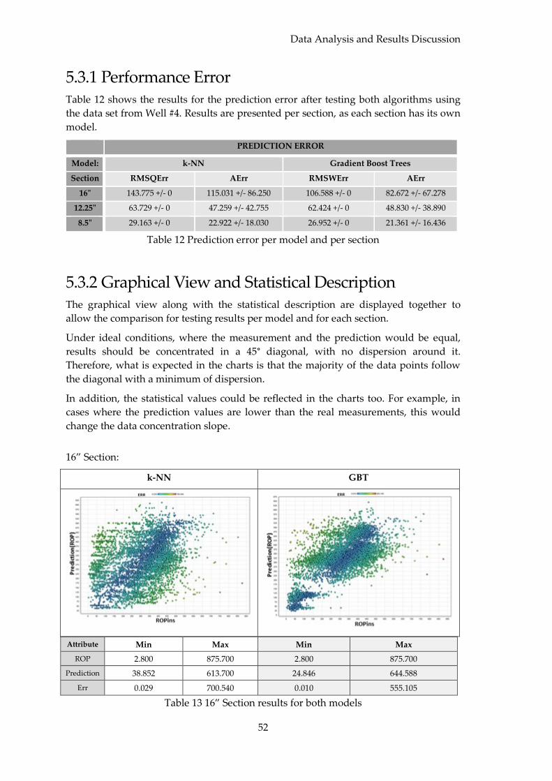
Data Analysis and Results Discussion
52
5.3.1 Performance Error Table 12 shows the results for the prediction error after testing both algorithms using
the data set from Well #4. Results are presented per section, as each section has its own
model.
PREDICTION ERROR
Model: k-NN Gradient Boost Trees
Section RMSQErr AErr RMSWErr AErr
16" 143.775 +/- 0 115.031 +/- 86.250 106.588 +/- 0 82.672 +/- 67.278
12.25" 63.729 +/- 0 47.259 +/- 42.755 62.424 +/- 0 48.830 +/- 38.890
8.5" 29.163 +/- 0 22.922 +/- 18.030 26.952 +/- 0 21.361 +/- 16.436
Table 12 Prediction error per model and per section
5.3.2 Graphical View and Statistical Description The graphical view along with the statistical description are displayed together to
allow the comparison for testing results per model and for each section.
Under ideal conditions, where the measurement and the prediction would be equal,
results should be concentrated in a 45° diagonal, with no dispersion around it.
Therefore, what is expected in the charts is that the majority of the data points follow
the diagonal with a minimum of dispersion.
In addition, the statistical values could be reflected in the charts too. For example, in
cases where the prediction values are lower than the real measurements, this would
change the data concentration slope.
16” Section:
k-NN GBT
Attribute Min Max Min Max
ROP 2.800 875.700 2.800 875.700
Prediction 38.852 613.700 24.846 644.588
Err 0.029 700.540 0.010 555.105
Table 13 16” Section results for both models
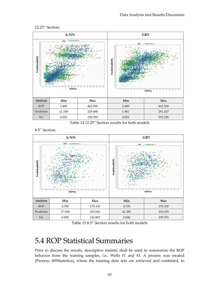
Data Analysis and Results Discussion
53
12.25” Section:
k-NN GBT
Attribute Min Max Min Max
ROP 2.400 462.500 2.400 462.500
Prediction 11.189 329.498 1.961 291.037
Err 0.023 256.589 0.001 253.256
Table 14 12.25” Section results for both models
8.5” Section:
k-NN GBT
Attribute Min Max Min Max
ROP 4.700 170.100 4.700 170.100
Prediction 17.944 103.942 41.281 102.039
Err 0.008 126.803 0.040 109.576
Table 15 8.5” Section results for both models
5.4 ROP Statistical Summaries Prior to discuss the results, descriptive statistic shall be used to summarize the ROP
behavior from the training samples, i.e., Wells #1 and #3. A process was created
(Process: 005Statistics), where the training data sets are retrieved and combined, to
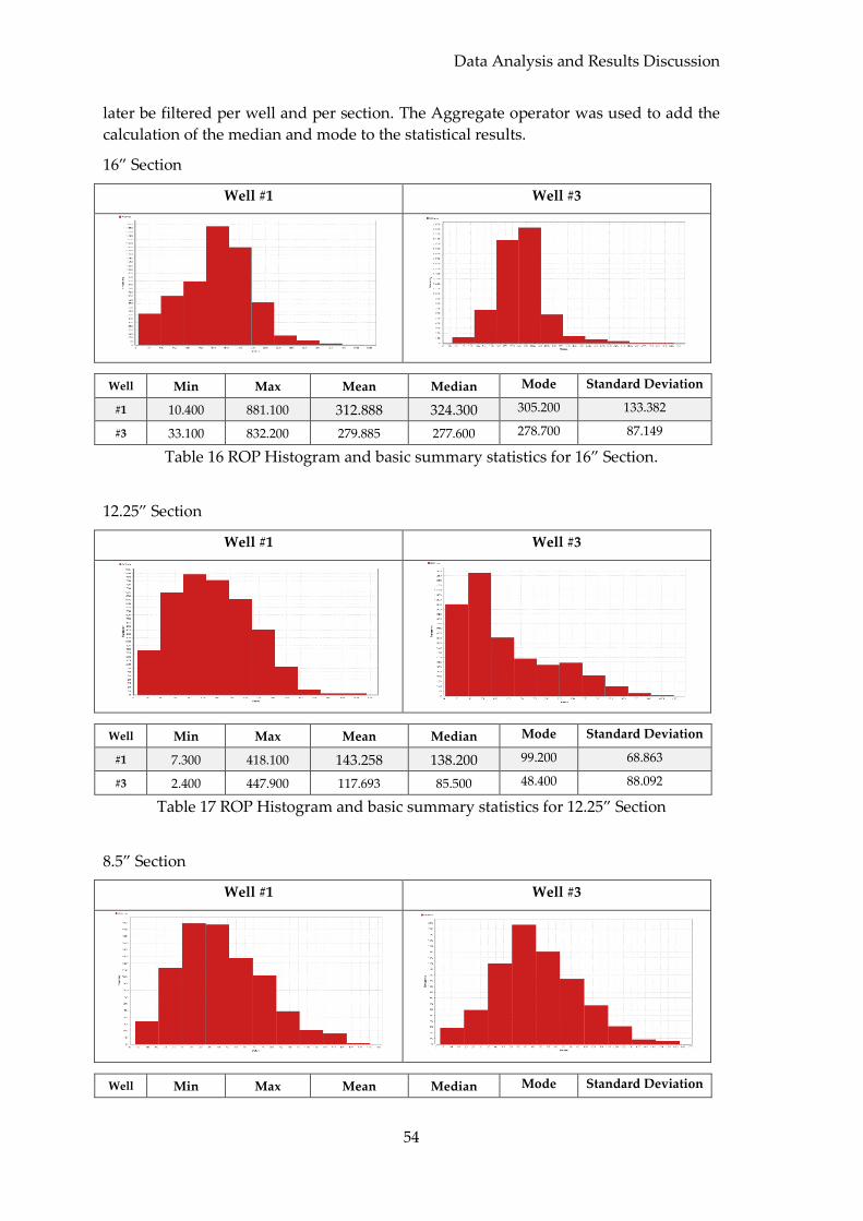
Data Analysis and Results Discussion
54
later be filtered per well and per section. The Aggregate operator was used to add the
calculation of the median and mode to the statistical results.
16” Section
Well #1 Well #3
Well Min Max Mean Median Mode Standard Deviation
#1 10.400 881.100 312.888 324.300 305.200 133.382
#3 33.100 832.200 279.885 277.600 278.700 87.149
Table 16 ROP Histogram and basic summary statistics for 16” Section.
12.25” Section
Well #1 Well #3
Well Min Max Mean Median Mode Standard Deviation
#1 7.300 418.100 143.258 138.200 99.200 68.863
#3 2.400 447.900 117.693 85.500 48.400 88.092
Table 17 ROP Histogram and basic summary statistics for 12.25” Section
8.5” Section
Well #1 Well #3
Well Min Max Mean Median Mode Standard Deviation
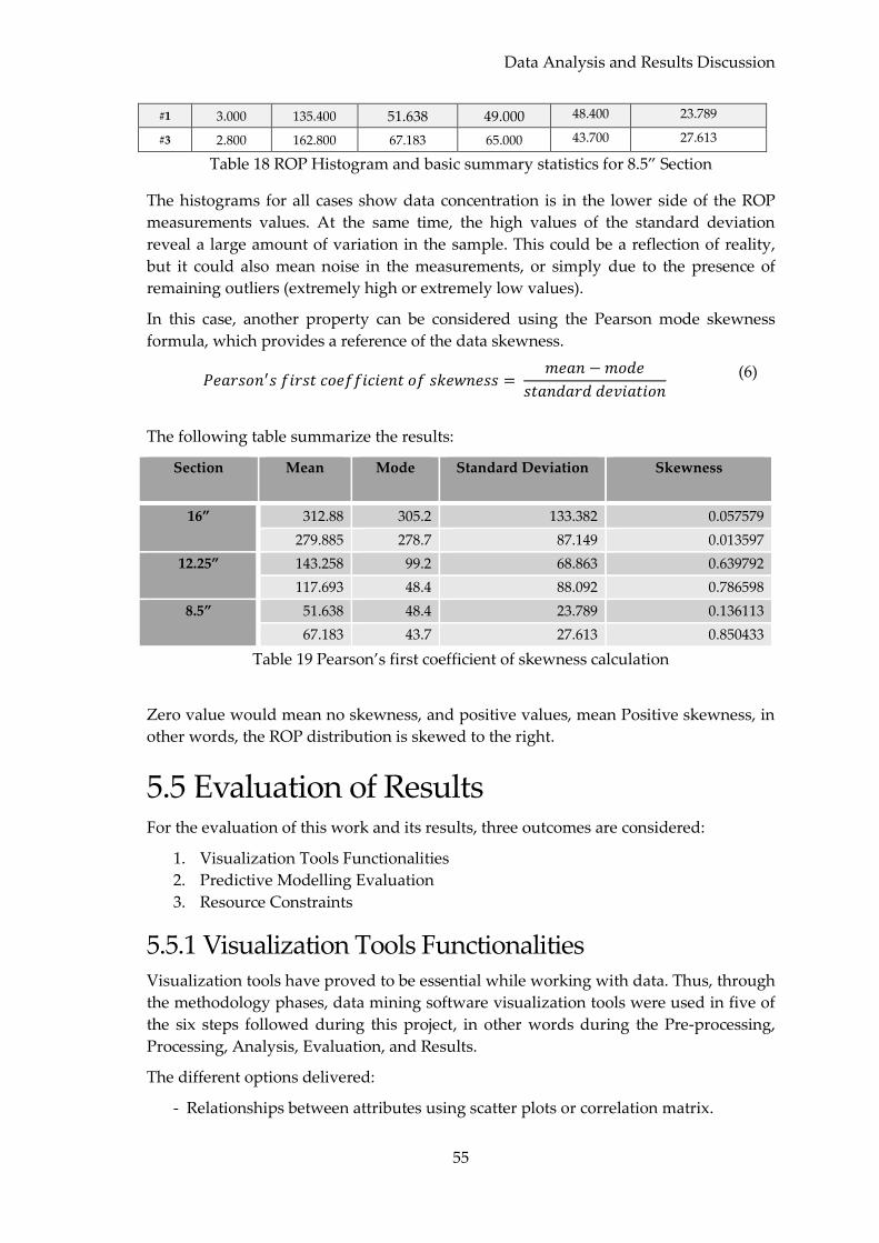
Data Analysis and Results Discussion
55
#1 3.000 135.400 51.638 49.000 48.400 23.789
#3 2.800 162.800 67.183 65.000 43.700 27.613
Table 18 ROP Histogram and basic summary statistics for 8.5” Section
The histograms for all cases show data concentration is in the lower side of the ROP
measurements values. At the same time, the high values of the standard deviation
reveal a large amount of variation in the sample. This could be a reflection of reality,
but it could also mean noise in the measurements, or simply due to the presence of
remaining outliers (extremely high or extremely low values).
In this case, another property can be considered using the Pearson mode skewness
formula, which provides a reference of the data skewness.
𝑃𝑒𝑎𝑟𝑠𝑜𝑛′𝑠 𝑓𝑖𝑟𝑠𝑡 𝑐𝑜𝑒𝑓𝑓𝑖𝑐𝑖𝑒𝑛𝑡 𝑜𝑓 𝑠𝑘𝑒𝑤𝑛𝑒𝑠𝑠 = 𝑚𝑒𝑎𝑛 − 𝑚𝑜𝑑𝑒
𝑠𝑡𝑎𝑛𝑑𝑎𝑟𝑑 𝑑𝑒𝑣𝑖𝑎𝑡𝑖𝑜𝑛
(6)
The following table summarize the results:
Section Mean Mode Standard Deviation Skewness
16” 312.88 305.2 133.382 0.057579
279.885 278.7 87.149 0.013597
12.25” 143.258 99.2 68.863 0.639792
117.693 48.4 88.092 0.786598
8.5” 51.638 48.4 23.789 0.136113
67.183 43.7 27.613 0.850433
Table 19 Pearson’s first coefficient of skewness calculation
Zero value would mean no skewness, and positive values, mean Positive skewness, in
other words, the ROP distribution is skewed to the right.
5.5 Evaluation of Results For the evaluation of this work and its results, three outcomes are considered:
1. Visualization Tools Functionalities
2. Predictive Modelling Evaluation
3. Resource Constraints
5.5.1 Visualization Tools Functionalities Visualization tools have proved to be essential while working with data. Thus, through
the methodology phases, data mining software visualization tools were used in five of
the six steps followed during this project, in other words during the Pre-processing,
Processing, Analysis, Evaluation, and Results.
The different options delivered:
- Relationships between attributes using scatter plots or correlation matrix.
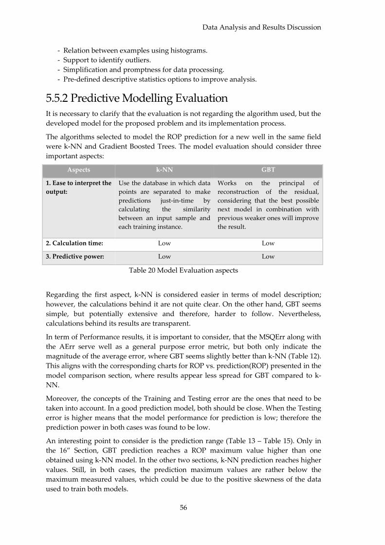
Data Analysis and Results Discussion
56
- Relation between examples using histograms.
- Support to identify outliers.
- Simplification and promptness for data processing.
- Pre-defined descriptive statistics options to improve analysis.
5.5.2 Predictive Modelling Evaluation It is necessary to clarify that the evaluation is not regarding the algorithm used, but the
developed model for the proposed problem and its implementation process.
The algorithms selected to model the ROP prediction for a new well in the same field
were k-NN and Gradient Boosted Trees. The model evaluation should consider three
important aspects:
Aspects k-NN GBT
1. Ease to interpret the
output:
Use the database in which data
points are separated to make
predictions just-in-time by
calculating the similarity
between an input sample and
each training instance.
Works on the principal of
reconstruction of the residual,
considering that the best possible
next model in combination with
previous weaker ones will improve
the result.
2. Calculation time: Low Low
3. Predictive power: Low Low
Table 20 Model Evaluation aspects
Regarding the first aspect, k-NN is considered easier in terms of model description;
however, the calculations behind it are not quite clear. On the other hand, GBT seems
simple, but potentially extensive and therefore, harder to follow. Nevertheless,
calculations behind its results are transparent.
In term of Performance results, it is important to consider, that the MSQErr along with
the AErr serve well as a general purpose error metric, but both only indicate the
magnitude of the average error, where GBT seems slightly better than k-NN (Table 12).
This aligns with the corresponding charts for ROP vs. prediction(ROP) presented in the
model comparison section, where results appear less spread for GBT compared to k-
NN.
Moreover, the concepts of the Training and Testing error are the ones that need to be
taken into account. In a good prediction model, both should be close. When the Testing
error is higher means that the model performance for prediction is low; therefore the
prediction power in both cases was found to be low.
An interesting point to consider is the prediction range (Table 13 – Table 15). Only in
the 16” Section, GBT prediction reaches a ROP maximum value higher than one
obtained using k-NN model. In the other two sections, k-NN prediction reaches higher
values. Still, in both cases, the prediction maximum values are rather below the
maximum measured values, which could be due to the positive skewness of the data
used to train both models.
Data Analysis and Results Discussion
57
Other important conclusion which related to the modelling evaluation and worth to be
mentioned here is: results show that prediction under specific conditions is possible,
but highly depending on the data availability for the model input, in two fronts:
quantity and quality.
For this project, the label attribute information was obtained in the form of a Depth
based LAS file with a granularity per foot. This could be improved when Time based
LAS files are available and for a fair amount of candidate wells.
It would also require an extensive quality control and higher processing power as
earlier exemplified in chapter 4.
5.5.3 Resource Constraints Finally, yet importantly, the resource constraints need to be mentioned and assessed,
starting with the data availability. Data mining reaches its potential based on its
capacity to handle huge amounts of data and extract useful information from it.
Unfortunately, for this study data was restricted in several ways:
- Samples, i.e., the number of well candidates was limited. The amount of
examples for 16” Section was much higher compared to the other two sections
(Table 8).
- Quality of the data. During the pre-processing stage, the data cleaning process
demanded extra QC work due to inconsistencies in the data. The outlier detection
was used for this aim through manual inspection and using an automated
detection operator (LOF distance).
- The geological attribute was the one including more missing values. It was not
complemented with a formation description to better feed the model.
- No metadata was available in the form of Daily Drilling Reports, Mud Reports,
Slide Sheets, Geological Reports, etc.
As equal in importance as data availability, is data understanding. Once the data is
obtained, understanding its format and the fields within it represents a challenge for
any outsider trying to analyse it. Particularly when not familiar with the data
acquisition process, which could result in unrepresentative data that would lead to
unpredictable results.

Data Analysis and Results Discussion
58
Conclusions & Recommendations
59
Chapter 6 Conclusions & Recommendations
6.1 Conclusions The main conclusions of the thesis can be summarized in the following points:
Referring to the overall process, extracting value from data should be
considered an iterative process that consists of specific phases, following clear
objectives with the corresponding acceptance criteria.
When working with real data, quality issues will always come across, where
the proper counter actions need to be put in place.
There are several software including different types of visualizations tools that
can be used in combination with descriptive statistics to increase efficiency
while performing data mining. However, in terms of processing, sufficient
computational power must be considered.
Data availability and its understanding are the main constraints for modelling
and prediction, along with the time frame needed to perform a good research
of the variable of concern and the data processing.
Training sets were summarized per section and using only the attributes that
could affect the outcome.
While performing algorithms selection, concepts need to be clear, considering
the “No Free Lunch Theorems for optimization”.
Model performance will vary depending on the amount of examples and
attributes, but typically requiring large volumes of training data to be effective.
In this context, data Pre-processing is essential to prepare a data set capable of
being mined in a reasonable amount of time without sacrificing accuracy.
k-NN model has two main parameters to be set: the distance measure method
used and the number of neighbours to choose. The number of neighbours is, in
fact, the most important parameter for this algorithm to perform properly, and
it is usually selected by training and evaluating the model.
GBT can slow the training process when lot of trees are used. In this regard,
optimization of parameters is needed to define a sweet spot involving the
maximum depth, because the deeper the tree, the more information it captures
about the data.
Performance optimization shows improvement in the prediction values for
both algorithms tested. However optimization was handled in different forms,
for:
- k-NN: a Cross Validation operator was used to optimize the model based
on random combinations of the training and testing sets from the original
sample.
- GBT: the performance optimization parameters functionality was used,
allowing evaluation of different model parameters, i.e., Maximum Depth
and Number of Trees, until the lower error were achieved.
Conclusions & Recommendations
60
6.2 Recommendations Based on the findings of this thesis the following recommendations can be drawn:
Data mining demands data quality. It is highly recommended that during the
data acquisition process, sensors’ operators get a clear understanding of their
role in constantly checking the sources of the data for accuracy. Most surface
sensors in the O&G industry still require often recalibration to avoid recording
null values or issuing readings with values physically not possible.
Furthermore, the implementation of Quality Control measurements for data
during acquisition and prior to delivery must become a standard procedure.
When possible, redundancy in the measurements should be considered, to
provide means for data validation, and to improve data quality.
It is suggested to assess the use of the Directional Difficulty Index (Oag W. and
Williams 2000), instead of some of the Directional Drilling attributes. This is due
to the differences in the ranges of values between attributes, which for
directional drilling attributes are considerable low compared to the other ones.
By reducing the difference between features values, attribute's weighting could
be prevented.
Consider a scalable infrastructure for high-density data, due to data acquisition
in two domains: depth and time. Additionally, balance of the data must be
taken into account to prevent effects on the validation of the performance.
Especial attention handling missing values is required, with focus in
understanding its type, possible effects and categorising how to do its
processing.
6.3 Further Work The main goal was to apply data mining to assess ROP response. Although this
objective was partially reached, mainly due to the resources constraints and the
resulted low prediction capability covered during the discussion of results, the
processes presented using drilling data endorse the application of data mining for ROP
analysis and prediction, where the further work should focus on:
Improving the prediction capability of the model, by overcoming its
uncertainty. A concept should be developed to generate uncertainty windows
for each predicted value.
Working through the cases where the actual ROP is below the predicted value.
Assessing the error per case, and as a group looking for common patterns.
Analyzing the factors contributing to the deviation from the reference.
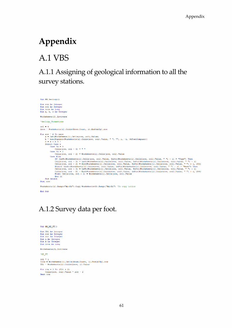
Appendix
61
Appendix
A.1 VBS
A.1.1 Assigning of geological information to all the
survey stations.
A.1.2 Survey data per foot.

Appendix
62
A.1.3 Geological data per foot.
A.1.4 Sections and tools used per foot
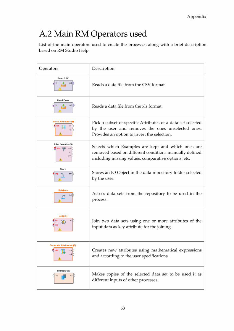
Appendix
63
A.2 Main RM Operators used List of the main operators used to create the processes along with a brief description
based on RM Studio Help:
Operators Description
Reads a data file from the CSV format.
Reads a data file from the xls format.
Pick a subset of specific Attributes of a data-set selected
by the user and removes the ones unselected ones.
Provides an option to invert the selection.
Selects which Examples are kept and which ones are
removed based on different conditions manually defined
including missing values, comparative options, etc.
Stores an IO Object in the data repository folder selected
by the user.
Access data sets from the repository to be used in the
process.
Join two data sets using one or more attributes of the
input data as key attribute for the joining.
Creates new attributes using mathematical expressions
and according to the user specifications.
Makes copies of the selected data set to be used it as
different inputs of other processes.
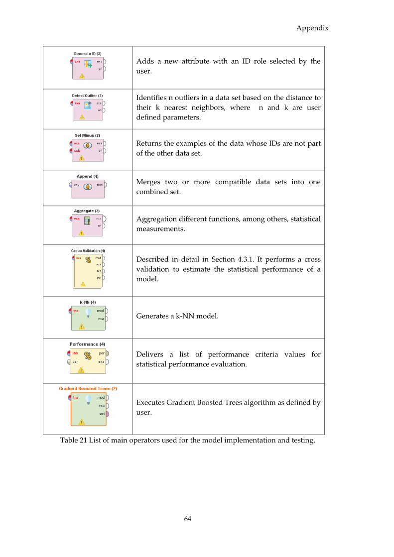
Appendix
64
Adds a new attribute with an ID role selected by the
user.
Identifies n outliers in a data set based on the distance to
their k nearest neighbors, where n and k are user
defined parameters.
Returns the examples of the data whose IDs are not part
of the other data set.
Merges two or more compatible data sets into one
combined set.
Aggregation different functions, among others, statistical
measurements.
Described in detail in Section 4.3.1. It performs a cross
validation to estimate the statistical performance of a
model.
Generates a k-NN model.
Delivers a list of performance criteria values for
statistical performance evaluation.
Executes Gradient Boosted Trees algorithm as defined by
user.
Table 21 List of main operators used for the model implementation and testing.
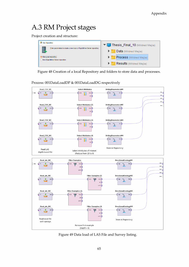
Appendix
65
A.3 RM Project stages Project creation and structure:
Figure 48 Creation of a local Repository and folders to store data and processes.
Process: 001DataLoadDP & 001DataLoadDG respectively
Figure 49 Data load of LAS File and Survey listing.
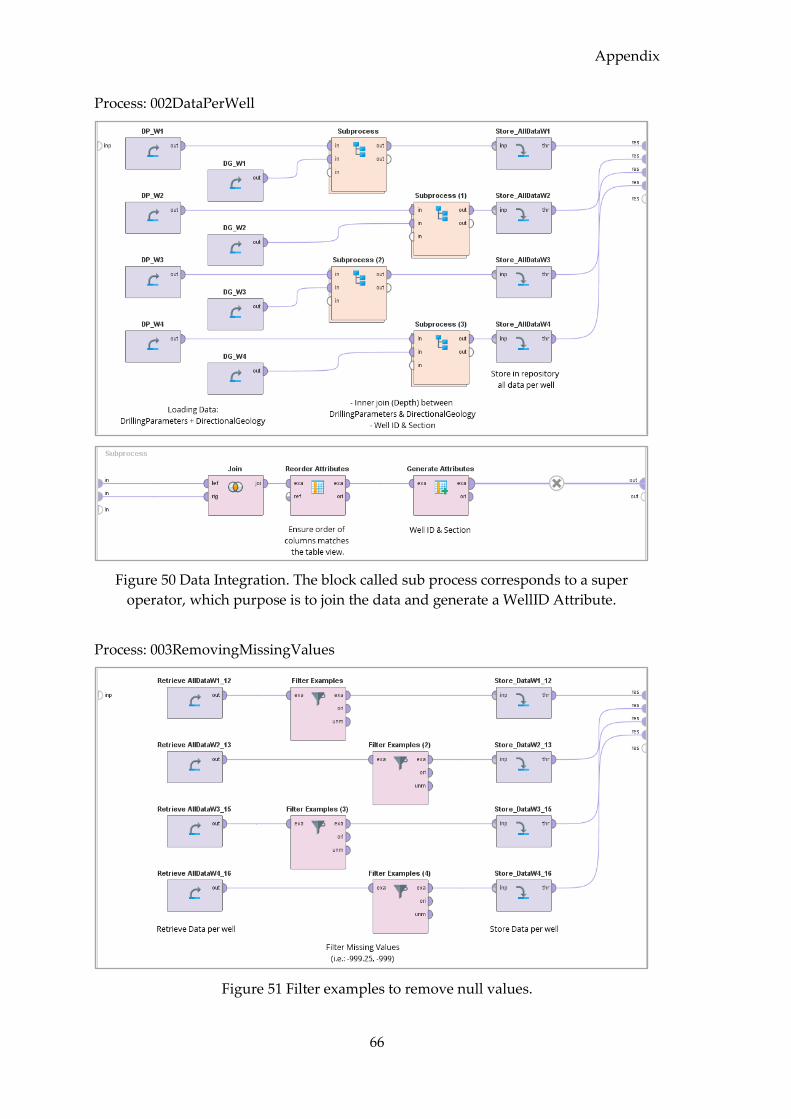
Appendix
66
Process: 002DataPerWell
Figure 50 Data Integration. The block called sub process corresponds to a super
operator, which purpose is to join the data and generate a WellID Attribute.
Process: 003RemovingMissingValues
Figure 51 Filter examples to remove null values.
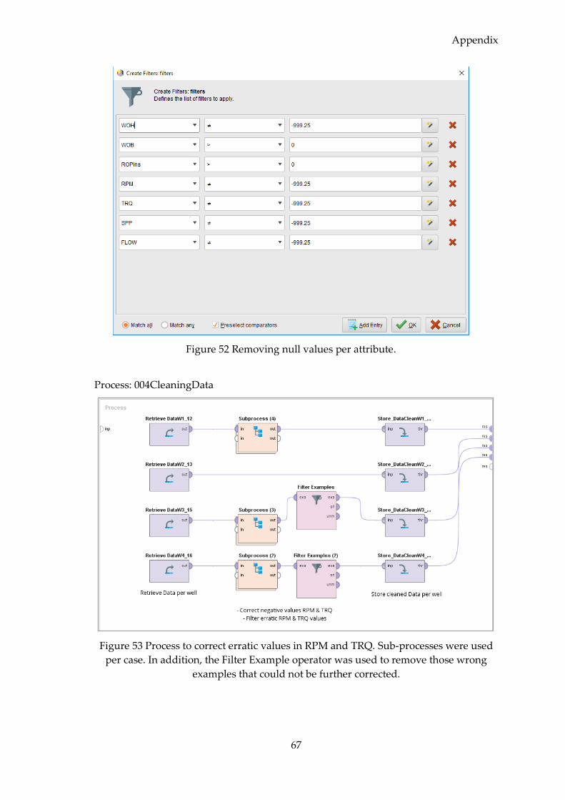
Appendix
67
Figure 52 Removing null values per attribute.
Process: 004CleaningData
Figure 53 Process to correct erratic values in RPM and TRQ. Sub-processes were used
per case. In addition, the Filter Example operator was used to remove those wrong
examples that could not be further corrected.
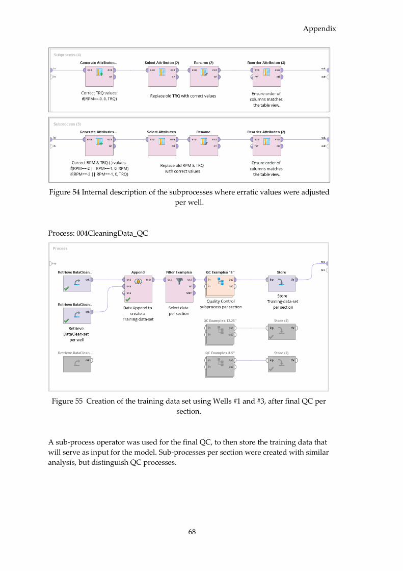
Appendix
68
Figure 54 Internal description of the subprocesses where erratic values were adjusted
per well.
Process: 004CleaningData_QC
Figure 55 Creation of the training data set using Wells #1 and #3, after final QC per
section.
A sub-process operator was used for the final QC, to then store the training data that
will serve as input for the model. Sub-processes per section were created with similar
analysis, but distinguish QC processes.
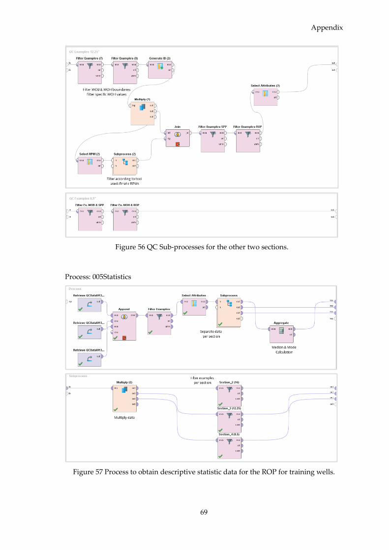
Appendix
69
Figure 56 QC Sub-processes for the other two sections.
Process: 005Statistics
Figure 57 Process to obtain descriptive statistic data for the ROP for training wells.
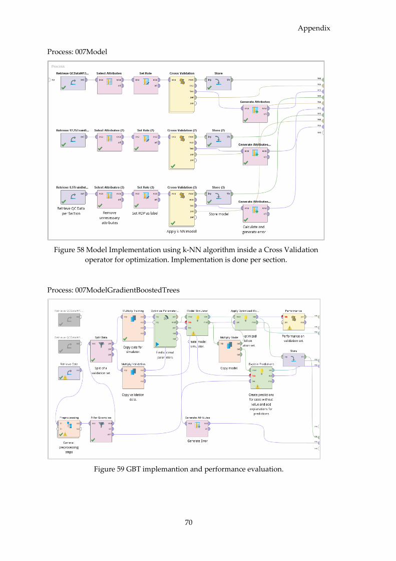
Appendix
70
Process: 007Model
Figure 58 Model Implementation using k-NN algorithm inside a Cross Validation
operator for optimization. Implementation is done per section.
Process: 007ModelGradientBoostedTrees
Figure 59 GBT implemantion and performance evaluation.
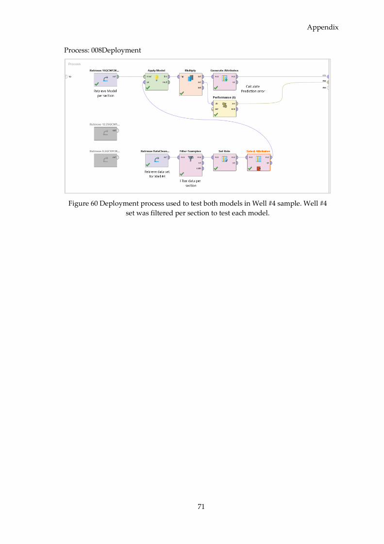
Appendix
71
Process: 008Deployment
Figure 60 Deployment process used to test both models in Well #4 sample. Well #4
set was filtered per section to test each model.

Appendix
72
Acronyms
73
Bibliography
Abou-Sayed, Ahmed. 2012. „Data Mining Applications in the Oil and Gas Industry.“
Journal of Petroleum Technology 88-95.
Asad, Elmgerbi. 2016. „Wellbore Position Planning # 1.“ Well Placement 590.017 Winter
Semester 2016/2017. Leoben: Montanuniveritaet, 17. November.
Azar, Jamal J., und G. Robello Samuel. 2007. Drilling Engineering. Tulsa, Oklahoma:
PennWell Corp.
Brownlee, Jason. 2016. „A Gentle Introduction to the Gradient Boosting Algorithm for
Machine Learning.“ Machine Learning Mastery. 09. September. Zugriff am 28.
April 2019. https://machinelearningmastery.com/gentle-introduction-gradient-
boosting-algorithm-machine-learning/.
Carden, Richard S. 2007. Horizontal and Directional Drilling. Tulsa, Oklahoma:
PetroSkills, LLC. An OGCI Company.
Donnelly, John. 2019. Journal of Petroleum Technology. 01. February. Zugriff am 6.
February 2019. (https://www.spe.org/en/jpt/jpt-article-
detail/?art=4976&utm_source=newsletter-jpt&utm_medium=email-
content&utm_campaign=JPT&utm_content=A%20Year%20of%20Uncertainty&
mkt_tok=eyJpIjoiWWpBNE1HUXlZelkxTWpVMiIsInQiOiJVZExQYll6aWdTN
DBrY0tJWXpCZzhDdlRVcXl5V1ZkbU.
Economides M. J., Watters L.T., Dunn-Norman S. 1997. Halliburton - Petroleum Well
Construction. Oklahoma: John Wiley and Sons.
Evans, Dean. 2017. IQ Intel: CognitiveComputing vs. Artificial Intelligence: What's the
Difference? 28. March. Zugriff am 12. February 2019.
https://iq.intel.co.uk/cognitive-computing-vs-artificial-intelligence/.
Gung. 2016. Stack Exchange - What is the difference between data mining, statistics, machine
learning and AI? 27. April. Zugriff am 17. June 2018.
https://stats.stackexchange.com/q/21669.
Han, Jiawei, und Micheline Kamber. 2006. Data mining. Concepts and techniques. . San
Francisco CA: Elsevier; Morgan Kaufmann.
I., Manuel. 2018. Top 33 Data mining software. NA. NA. Zugriff am 2. April 2018.
https://www.predictiveanalyticstoday.com/top-data-mining-software/.
IADC. 2014. IADC Drilling Manual. NA: IADC.
Jacobs, Trent. 2018. Journal of Petroleum Technology . 01. October. Zugriff am 2. February
2019. https://www.spe.org/en/jpt/jpt-article-detail/?art=4632.
—. 2019. Journal of Petroleum Technology. 04. February. Zugriff am 5. March 2019.
https://www.spe.org/en/jpt/jpt-article-detail/?art=5069&utm_source=newsletter-
jpt&utm_medium=email-
content&utm_campaign=JPT&utm_content=US%20Shale%20To%20Drill%20An
Acronyms
74
d%20Complete%2020%2C000%20Wells%20This%20Year&mkt_tok=eyJpIjoiW
WpBNE1HUXlZelkxTWpVMiIsInQiO.
Johnston, Joe, und Guichard Aurelien. 2015. „Using Big Data Analysis Tools to
Understand Bad Hole Sections on the UK Continental Shelf .“ Journal of
Petroleum Technology 60-63.
Knezevic, Rudofl. 2017. VO + UE measurement, control, monitoring & analysis. Handout,
Leoben: DPE.
Kuhn, Max, und Kjell Johnson. 2013. Applied Predictive Modeling. New York: Springer.
Li, Jin. 2017. „Assessing the accuracy of predictive models for numerical data: Not r
nor r2, why not? Then what?“ Plos One 5.
Maidla, Eric, William Maidla, John Rigg, Michael Crumrine, und Philipp Wolf-
Zoellner. 2018. Drilling Analysis Using Big Data has been Misused and Abused.
Paper, Fort Worth, Texas: IADC/SPE Drilling Conference and Exhibition.
Mensa-Wilmot, G., Y. Harjadi, S. Langdon, und J. Gagneaux. 2010. Drilling Efficiency
and Rate of Penetratiom - Definitions, Influencing Factors, Relationships and Value.
Paper, New Orleans, Luisiana: IADC/SPE Drilling Conference and Exhibition.
Mierswa, Ingo. kein Datum. rapidminer. Zugriff am 12. April 2018.
https://rapidminer.com/.
Nguyen, J. P. 1996. Drilling - Fundamentals of Exploration & Production. Paris: Editions
Technip.
Nivre, Joakim. 2007. Machine Learning - Basic Methodology. Presentation, Småland,
Sweden: Uppala University and Växjö University.
Oag W., Alistair, und Mike Williams. 2000. The Directional Difficulty Index - A New
Approach to Performance Benchmarking. IADC/SPE Drilling Conference , New
Orleans, Louisiana: Society of Petroleum Engineers.
Optima, Frank. 2017. Log Ascii Standard (LAS) Files. 01. October. Zugriff am 30. March
2019. http://www.frackoptima.com/userguide/interface/las.html.
Page, John. 2011. Math Open Reference. NA. NA. Zugriff am 19. April 2019.
https://www.mathopenref.com/real-number.html.
Parshall, Joel. 2015. „Drilling Data provide solution to Horizontal Well Log costs.“
Journal of Petroleum Technology - JPT. 01. August. Zugriff am 19. October 2018.
https://www.onepetro.org/download/journal-paper/SPE-0815-0035-
JPT?id=journal-paper%2FSPE-0815-0035-JPT.
Pinki, Sagar, P. Prinima, und I. Indu. 2017. „Analysis of Prediction Techniques based
on Classification and Regression.“ IJCA 163 47-41.
Platon, Radu, und Mouloud Amazouz. 2007. Application of Data Mining Techniques for
Industrial Process Optimization. A Literature and Software review. Natural
Resources Canada, Varennes. Canada.: CETC.
Press, Gil. 2016. „Forbes.“ Cleaning Big Data: Most Time-Consuming, Least Enjoyable Data
Science Task, Survey Says. 23. March. Zugriff am 25. March 2019.
Acronyms
75
https://www.forbes.com/sites/gilpress/2016/03/23/data-preparation-most-time-
consuming-least-enjoyable-data-science-task-survey-says/.
2019. Quantico Energy. Zugriff am 7/. February 2019.
http://www.quanticoenergy.com/#news.
Rapidminer. 2014. „RapidMiner Studio Manual.“ Global leader in predictive analytics
software. Boston: www.rapidminer.com, NA. NA.
Ray, Sunil. 2015. Analytics Vidhya - Types of Regression Techniques. 14. August. Zugriff
am 29. April 2019.
https://www.analyticsvidhya.com/blog/2015/08/comprehensive-guide-
regression/.
Solesa, M. 2017. „Well Monitoring and Analysis.“ Lecture Notes "Well Monitoring and
Analysis". Leoben: Montan Universitaet Leoben, 1. November.
Tan, Pang-Ning, Michael Steinbach, und Vipin Kumar. 2006. Introduction to data mining.
Boston: Pearson Education.
Witten, Ian H., und Eibe. Frank. 2005. Data Mining: Practical Machine Learning Tools and
Techniques. San Francisco, CA.: Elsevier.
Wolpert, David H., und Willam G. Macready. 1997. „No Free Lunch Theorems for
Optimization.“ IEEE Transactions on Evolutionary Computation Vol. 1, No. 1.
Zhang, Barry. 2018. 2. January . Zugriff am 5. February 2019.
http://www.quanticoenergy.com/#news.

Acronyms
76
Acronyms
77
Acronyms
ROP
O&G
VBS
WOB
WOH
SPP
TVD
DLS
BR
TR
RM
RSS
k-NN
RMSQErr
AErr
GBT
KDD
NGL
QC
Rate of Penetration
Oil and Gas
Visual Basic Script
Weight on Bit
Weight on Hook
Standpipe pressure
True Vertical Depth
Dogleg Severity
Build-Rate
Turn-Rate
RapidMiner Studio
Rotary Steerable System
k-Nearest Neighbours
Root Mean Square Error
Absolute Error
Gradient Boost Trees
Knowledge Discovery from Data
Natural Gas Liquid
Quality Control

Symbols
78
Symbols
𝐼 Inclination [degrees]
𝐴
ds
Azimuth
Course length
[degrees]
[ft. or m]
n number of examples in a data set [ - ]
𝑦𝑖 observed value for i-example [depends on example]
�̅�𝑖 prediction for i-example [depends on example]
List of Figures
79
List of Figures
Figure 1 Wells drilled, completed, and drilled-but-uncompleted per year until 2018. Projection
until 2022 (Jacobs, Journal of Petroleum Technology 2019) ..................................................... 2 Figure 2 Workflow divided in four specific phases ............................................................................ 2 Figure 3 Data Mining system (Abou-Sayed 2012) ................................................................................ 3 Figure 4 Plot of customer data in relation to its location in a city. Three data clusters are clearly
identified (Han and Kamber 2006) ................................................................................................ 7 Figure 5 Beyond Limits Reservoir Management advisor (Jacobs, Journal of Petroleum
Technology 2018) ........................................................................................................................... 10 Figure 6 Anomaly Detection: A high risk situation was identified (Johnston and Aurelien 2015)
.......................................................................................................................................................... 11 Figure 7 Differences were less than the precision of the logging tools, where Real Time
measuremets are highly depended of the hole conditions and largely affected by hole
washouts (Zhang 2018) ................................................................................................................. 13 Figure 8 Results of survey between data scientists showing the time needed to massage the data
prior its use (Press 2016) ............................................................................................................... 19 Figure 9 Pressure Transducer installed in manifold on the rig floor ............................................... 20 Figure 10 Hookload sensor installed in the drill line ......................................................................... 20 Figure 11 General structure for the methodology .............................................................................. 21 Figure 12 Phases for the workflow ....................................................................................................... 21 Figure 13 The majority of the Header Section was not provided due to confidentiality reasons 24 Figure 14 Example of a Survey Report ................................................................................................. 24 Figure 15 Example of a BHA Configuration Report. ........................................................................ 25 Figure 16 Steps of the Pre-processing stage ........................................................................................ 26 Figure 17 Software selection criteria .................................................................................................... 26 Figure 18 Rapidminer Studio Operators Library classification. Example of an Operator along
with the Input/Output descriptions ............................................................................................ 27 Figure 19 Data view through Examples, regular and special attributes ........................................ 28 Figure 20 Example of the content of the Survey Report, showing only the attributes of interest at
specific depths................................................................................................................................ 29 Figure 21 Workflow implemented in VBS to transform the data into the desired granularity ... 29 Figure 22 Directional and Geological Data per foot. ......................................................................... 30 Figure 23 Project structure in RM ........................................................................................................ 31 Figure 24 Flowchart to load Drilling, Directional and Geological parameters .............................. 31 Figure 25 Attribute Generator operator applications ........................................................................ 32 Figure 26 RM Data visualization options ............................................................................................ 34 Figure 27 Statistical Visualization of the data ..................................................................................... 34 Figure 28 Part of the process to remove the null values -999.25. Description of the content inside
the Filter Example operator, where conditions can be set as required and per attribute .... 35 Figure 29 Inconsistency in TRQ values in relation to RPM values .................................................. 35 Figure 30 Depth vs. RPM based on the tool used. .............................................................................. 36 Figure 31 Depth vs. RPM & TRQ .......................................................................................................... 36 Figure 32 Depth vs. RPM in contrast with the Inclination in colos scale ........................................ 37 Figure 33 QC sub-process to prepare the 16” training set ................................................................. 38 Figure 34 The left chart shows data for WOH before the QC process. The right chart show the
data once removing the unreliable values (59 Examples were removed) ............................. 39 Figure 35 The first chart shows the RPM values in relation to the tool used. The second chart
shows in red the values calculated as outliers........................................................................... 39
List of Figures
80
Figure 36 k-NN model using a Cross Validation operator for optimization. Sub-process inside
the Cross Validation operator: the left side is the training part for the model, and the right
side is the testing part and performance evaluation ................................................................. 41 Figure 37 ROP vs. prediction(ROP) using k-NN for 16” Section training set. In colour scale is the
generated difference between both values, suggesting the tendency for a straight line as
wanted ............................................................................................................................................. 43 Figure 38 Depth vs. Error using k-NN in 16” Section ........................................................................ 44 Figure 39 Statistical summarize of results using k-NN in 16” Section ............................................ 44 Figure 40 Auto Model sequential workflow ....................................................................................... 44 Figure 41 Model Types step ................................................................................................................... 45 Figure 42 Auto Model results comparisson ......................................................................................... 45 Figure 43 Graphical visualization of the Performance for Parameters and table of Performance47 Figure 44 Gradient Boosted Trees model with restricted parameters. First tree ............................ 47 Figure 45 The two remaining trees that complete the model for the limited case ......................... 47 Figure 46 Left: ROP vs. prediction(ROP). Generated Error in colour scale. Right: Depth vs. Error
.......................................................................................................................................................... 48 Figure 47 Statistical data for a) The measured ROP, b) The predicted ROP, and c) The Error .... 49 Figure 48 Creation of a local Repository and folders to store data and processes. ........................ 65 Figure 49 Data load of LAS File and Survey listing. .......................................................................... 65 Figure 50 Data Integration. The block called sub process corresponds to a super operator, which
purpose is to join the data and generate a WellID Attribute. .................................................. 66 Figure 51 Filter examples to remove null values. ............................................................................... 66 Figure 52 Removing null values per attribute. .................................................................................... 67 Figure 53 Process to correct erratic values in RPM and TRQ. Sub-processes were used per case.
In addition, the Filter Example operator was used to remove those wrong examples that
could not be further corrected. .................................................................................................... 67 Figure 54 Internal description of the subprocesses where erratic values were adjusted per well.
.......................................................................................................................................................... 68 Figure 55 Creation of the training data set using Wells #1 and #3, after final QC per section. ... 68 Figure 56 QC Sub-processes for the other two sections. .................................................................... 69 Figure 57 Process to obtain descriptive statistic data for the ROP for training wells. ................... 69 Figure 58 Model Implementation using k-NN algorithm inside a Cross Validation operator for
optimization. Implementation is done per section. .................................................................. 70 Figure 59 GBT implemantion and performance evaluation. ............................................................. 70 Figure 60 Deployment process used to test both models in Well #4 sample. Well #4 set was
filtered per section to test each model. ....................................................................................... 71
List of Tables
81
List of Tables
Table 1 Summary of Attributes coming from surface sensors .......................................................... 16 Table 2 Attribute related to the directional work ............................................................................... 16 Table 3 Well candidates’ basic details. All units related to distances are in feet [ft] ..................... 22 Table 4 () Available file, () Unavailable file.................................................................................... 23 Table 5 Summarize of the value types used in the data sets. ............................................................ 28 Table 6 Summarize of Attributes including unit of measurement and data type......................... 33 Table 7 Well data set including deflection tool per run ..................................................................... 38 Table 8 Training sets per section after QC ........................................................................................... 40 Table 9 Basic guideline to select the task. ............................................................................................ 40 Table 10 RMSQErr and AErr for all sections using k-NN ................................................................. 43 Table 11 RMSQErr and AErr for all sections using optimized GBT. ............................................... 48 Table 12 Prediction error per model and per section ......................................................................... 52 Table 13 16” Section results for both models ...................................................................................... 52 Table 14 12.25” Section results for both models ................................................................................. 53 Table 15 8.5” Section results for both models ..................................................................................... 53 Table 16 ROP Histogram and basic summary statistics for 16” Section.......................................... 54 Table 17 ROP Histogram and basic summary statistics for 12.25” Section ..................................... 54 Table 18 ROP Histogram and basic summary statistics for 8.5” Section......................................... 55 Table 19 Pearson’s first coefficient of skewness calculation ............................................................. 55 Table 20 Model Evaluation aspects ...................................................................................................... 56 Table 21 List of main operators used for the model implementation and testing. ........................ 64