application of dilation invariance principle in eddy
TRANSCRIPT
Application of Dilation Invariance Principle in Eddy-currentNondestructive Testing
Prashanth Baskaran
Thesis to obtain the Master of Science Degree in
Electrical and Computer Engineering
Supervisor(s): Prof. Helena Maria dos Santos Geirinhas RamosProf. Artur Fernando Delgado Lopes Ribeiro
Examination Committee
Chairperson: Prof. Gonçalo Nuno Gomes TavaresSupervisor: Prof. Helena Maria dos Santos Geirinhas Ramos
Member of the Committee: Prof. Francisco André Corrêa Alegria
July 2017

ii

Acknowledgments
This work was developed under the Instituto de Telecomunicacoes project EvalTubes and supported in part by the
Portuguese Science and Technology Foundation (FCT) project: UID/EEA/50008/2013.
iii

iv

Abstract
The objective of this dissertation is a proof of concept on the possibility to measure the same magnetic fields,
by the principle of dilation invariance, using eddy current non-destructive testing technique. According to this
principle, dilation of the dimensional and electrical parameters of a probe and a plate with crack reproduces the
same magnetic field (measured at every dilated point) which was produced by a probe and a plate with crack,
without dilation. This implies that, in order to evaluate the performance of eddy current method in a specific
industrial case study, one can carry out tests in a scaled model in the laboratory and then, extend the conclusions
to the real situation by using dilation invariance principle. The experimental and simulation results show a good
agreement of crack detection by using two eddy current probes of which one is the dilated version of the other. The
work has been analytically supported by considering a simpler case of an axially symmetric geometry, without a
crack. The resulting equations of the magnetic flux density are evaluated numerically using stratified Monte Carlo
numerical integration technique.
Keywords
ECT; eddy current testing; nondestructive evaluation; dilation invariance principle; Maxwell equations; magnetic
field; magnetic vector potential; eddy-currents.
v

vi
Contents
Acknowledgments . . . . . . . . . . . . . . . . . . . . . . . . . . . . . . . . . . . . . . . . . . . . . . iii
Abstract . . . . . . . . . . . . . . . . . . . . . . . . . . . . . . . . . . . . . . . . . . . . . . . . . . . v
List of Tables . . . . . . . . . . . . . . . . . . . . . . . . . . . . . . . . . . . . . . . . . . . . . . . . ix
List of Figures . . . . . . . . . . . . . . . . . . . . . . . . . . . . . . . . . . . . . . . . . . . . . . . . xi
Nomenclature . . . . . . . . . . . . . . . . . . . . . . . . . . . . . . . . . . . . . . . . . . . . . . . . xiii
Glossary . . . . . . . . . . . . . . . . . . . . . . . . . . . . . . . . . . . . . . . . . . . . . . . . . . . xiii
1 Dilation Invariance Theory 1
1.1 Purpose of the Study . . . . . . . . . . . . . . . . . . . . . . . . . . . . . . . . . . . . . . . . . 1
1.2 Dilation Invariance Principle . . . . . . . . . . . . . . . . . . . . . . . . . . . . . . . . . . . . . 2
1.3 State of the Art . . . . . . . . . . . . . . . . . . . . . . . . . . . . . . . . . . . . . . . . . . . . 3
2 Introduction to Eddy Current Non Destructive Testing 5
2.1 Eddy Current and Skin Effect . . . . . . . . . . . . . . . . . . . . . . . . . . . . . . . . . . . . . 6
2.2 Eddy Current Testing . . . . . . . . . . . . . . . . . . . . . . . . . . . . . . . . . . . . . . . . . 7
2.3 Eddy Current Probes . . . . . . . . . . . . . . . . . . . . . . . . . . . . . . . . . . . . . . . . . 8
2.4 Measurements . . . . . . . . . . . . . . . . . . . . . . . . . . . . . . . . . . . . . . . . . . . . . 8
2.5 Parameters Affecting the Magnitude of Eddy Current Response . . . . . . . . . . . . . . . . . . . 9
2.6 Potential Applications of ECT . . . . . . . . . . . . . . . . . . . . . . . . . . . . . . . . . . . . 9
2.7 Advantages of ECT . . . . . . . . . . . . . . . . . . . . . . . . . . . . . . . . . . . . . . . . . . 9
2.8 Disadvantages of ECT . . . . . . . . . . . . . . . . . . . . . . . . . . . . . . . . . . . . . . . . 10
2.9 Formulation of the Dilation Parameters . . . . . . . . . . . . . . . . . . . . . . . . . . . . . . . . 10
3 Simulation of the study 13
3.1 Advantages of Simulation . . . . . . . . . . . . . . . . . . . . . . . . . . . . . . . . . . . . . . . 13
3.2 Disadvantages of Simulation . . . . . . . . . . . . . . . . . . . . . . . . . . . . . . . . . . . . . 14
3.3 Dimensional and Electrical Specifications . . . . . . . . . . . . . . . . . . . . . . . . . . . . . . 14
3.4 Simulation Measures and Considerations . . . . . . . . . . . . . . . . . . . . . . . . . . . . . . . 15
3.5 Current Density Around the Notch . . . . . . . . . . . . . . . . . . . . . . . . . . . . . . . . . . 16
4 Experimentation of the Study 19
4.1 Description of Case Studies . . . . . . . . . . . . . . . . . . . . . . . . . . . . . . . . . . . . . . 19
vii
4.2 Dimension and Electrical Specification of the Probe, Plate and the Crack . . . . . . . . . . . . . . 20
4.3 Experimental Setup . . . . . . . . . . . . . . . . . . . . . . . . . . . . . . . . . . . . . . . . . . 20
5 Discussion 23
5.1 Results from Experiment . . . . . . . . . . . . . . . . . . . . . . . . . . . . . . . . . . . . . . . 23
5.2 Results from Simulation . . . . . . . . . . . . . . . . . . . . . . . . . . . . . . . . . . . . . . . 24
6 Analytical Verification to Dilation Invariance Problem 27
6.1 Field Equation . . . . . . . . . . . . . . . . . . . . . . . . . . . . . . . . . . . . . . . . . . . . . 27
6.2 Formulation of the Field Equation . . . . . . . . . . . . . . . . . . . . . . . . . . . . . . . . . . 28
6.3 Solution for the Field Equation . . . . . . . . . . . . . . . . . . . . . . . . . . . . . . . . . . . . 30
6.4 Invariance of Magnetic Field . . . . . . . . . . . . . . . . . . . . . . . . . . . . . . . . . . . . . 44
7 Conclusions 51
7.1 Experimental Study . . . . . . . . . . . . . . . . . . . . . . . . . . . . . . . . . . . . . . . . . . 51
7.2 Simulation Study . . . . . . . . . . . . . . . . . . . . . . . . . . . . . . . . . . . . . . . . . . . 51
7.3 Analytical Study . . . . . . . . . . . . . . . . . . . . . . . . . . . . . . . . . . . . . . . . . . . 52
Bibliography 53
A Stratified Monte Carlo Numerical integration 55
A.1 Computation of Magnetic Flux Density . . . . . . . . . . . . . . . . . . . . . . . . . . . . . . . 55
B Dilation of parameters 58
C Domain Meshing and Assembly 61
viii

List of Tables
4.1 Geometrical Specification for study1 and study2 . . . . . . . . . . . . . . . . . . . . . . . . . . . 20
4.2 Electrical Specification for study1 and study2 . . . . . . . . . . . . . . . . . . . . . . . . . . . . 20
ix

x

List of Figures
2.1 Decay of eddy current density inside the specimen for the case of constant surface current density. 6
3.1 Geometry of the ECT implemented in Comsol. . . . . . . . . . . . . . . . . . . . . . . . . . . . 14
3.2 High density mesh region situated in between the air and probe region. . . . . . . . . . . . . . . . 16
3.3 Eddy currents in (a) the absence of a crack (b) the presence of crack . . . . . . . . . . . . . . . . 17
3.4 Magnetic flux density (B) obtained by simulation . . . . . . . . . . . . . . . . . . . . . . . . . . 17
4.1 The experimental setup . . . . . . . . . . . . . . . . . . . . . . . . . . . . . . . . . . . . . . . . 21
5.1 Horizontal scan result . . . . . . . . . . . . . . . . . . . . . . . . . . . . . . . . . . . . . . . . . 23
5.2 Vertical scan result . . . . . . . . . . . . . . . . . . . . . . . . . . . . . . . . . . . . . . . . . . 24
5.3 Horizontal scan result . . . . . . . . . . . . . . . . . . . . . . . . . . . . . . . . . . . . . . . . . 24
5.4 Vertical scan result . . . . . . . . . . . . . . . . . . . . . . . . . . . . . . . . . . . . . . . . . . 25
5.5 plot of Bz . . . . . . . . . . . . . . . . . . . . . . . . . . . . . . . . . . . . . . . . . . . . . . . 25
6.1 The 2-D Axi-symmetric model of 2 conducting plates with a surface probe excited by a current
source pointing inside the page. . . . . . . . . . . . . . . . . . . . . . . . . . . . . . . . . . . . . 29
6.2 A delta function coil placed over 2 conducting plates. . . . . . . . . . . . . . . . . . . . . . . . . 31
6.3 Integrating the DFCs over a region . . . . . . . . . . . . . . . . . . . . . . . . . . . . . . . . . . 40
6.4 Pictorial representation of the problem in new co-ordinates and selecting the sub-regions for com-
puting A1−2φ
(r,z) . . . . . . . . . . . . . . . . . . . . . . . . . . . . . . . . . . . . . . . . . . . 43
6.5 Summing the solution of a DFC, first along ζ and then along r . . . . . . . . . . . . . . . . . . . 43
6.6 Histogram plot of distribution of points in each stratum . . . . . . . . . . . . . . . . . . . . . . . 46
6.7 Surface plot of Magnetic Flux Density for k = 1 . . . . . . . . . . . . . . . . . . . . . . . . . . . 47
6.8 Srface plot of magnetic flux density for k = 4 . . . . . . . . . . . . . . . . . . . . . . . . . . . . 49
6.9 Numerical Integration error for k = 1 . . . . . . . . . . . . . . . . . . . . . . . . . . . . . . . . . 50
6.10 Ratio of the absolute values of the individual components of the magnetic flux density . . . . . . . 50
C.1 Plate with crack . . . . . . . . . . . . . . . . . . . . . . . . . . . . . . . . . . . . . . . . . . . . 61
C.2 Probe . . . . . . . . . . . . . . . . . . . . . . . . . . . . . . . . . . . . . . . . . . . . . . . . . 62
C.3 Reference edge for orientation (in blue) and direction (red arrow) of current in the coil . . . . . . 62
C.4 Assembly of probe, plate with notch and the high density mesh region . . . . . . . . . . . . . . . 63
C.5 Assembly of probe, plate with notch, high density mesh region and the boundary domain . . . . . 63
xi

xii

Glossary
DFC Delta Function Coil.
ECT Eddy Current Testing.
EMF Electromotive Force.
MMF Magnetomotive Force.
MVP Magnetic Vector Potential.
NDT Non Destructive Testing.
xiii

xiv
Chapter 1
Dilation Invariance Theory
In this chapter of the thesis, we are going to discuss about the motivation of the problem and its potential applica-
tions in industries. After a brief introduction, the formal statement of the principle is proposed. With this in mind
we are going to introduce the state of the art of the work that was carried out by listing the previous work that was
performed applying this principle and we also explain in detail how the previous work was extended.
1.1 Purpose of the Study
In certain industries, such as petroleum industries, nuclear industries, etc. in order to carry fluids, pipelines are
used. These pipelines in some cases are electrically conductive materials. In the case of nuclear industry, the heat
exchangers are made of thermally conductive materials such as aluminium or stainless steel in order to maximize
the heat transfer. In these cases the materials undergo lot of stress at higher pressure and temperature. This may
cause development of fatigue/cracks from inside the pipes. These pipes are usually thick and the outer diameter
may be more than ten centimeters and inner diameter may be about eight centimeters. This makes the thickness of
the pipe to be more than one centimeter.
Since these materials are subject to harsh environments [20], it is recommended to test for the presence of
defects or any other anomalies periodically. It is also not recommended to destroy the materials to test for the
presence of anomalies. It is because it may or may not have an anomaly. So it is recommended to perform tests
without destroying them. Hence NDT methods are preferred in such situations.
Even though there are various methods of NDT the preferred ones are ECT and Ultrasonic testing. Since these
materials are thermally as well as electrically conductive, ECT is a preferred technique. It is because the surface
of the probe need not be in contact with the materials.
Most of the small scale industries do not have specialized department that have dedicated lab for testing and
analysing the materials periodically. So, those samples has to be sent to the organizations that involve in NDT in-
spections. Transportation of such huge structures is not practically possible and also the thickness being very high,
1

eddy current probes that needs to be designed to test the samples are relatively bigger. Building thicker probes in
small labs is a difficult task.
This thesis comes up with an idea to build an eddy current probe for a scaled version of sample so that eddy
current probes of relatively smaller sizes can be built in the lab (provided the feasibility of the study in the labora-
tory). Testing can be made using the scaled (dilated) version of the probe on the scaled version of the sample for
an artificially created notch. So using the specified electrical and dimensional parameters for the probe, the bigger
probe can be constructed and can be used for testing in the industry. If the dilation parameters are obeyed, then the
magnetic field sensed by a sensor in the probe will be the same for the original and the dilated version of the crack.
1.2 Dilation Invariance Principle
The statement of the principle is formally given as -
Dilation of the dimensional and electrical parameters of a probe and a plate with crack reproduces the same
magnetic field (measured at every dilated point) which was produced by a probe and a plate with crack, without
dilation.
The intended application behind the principle is to detect same magnetic field in the case of non-dilated version
(original sample) and the dilated version (testing sample). So basically the thickness of the sample is dilated to a
version that is less than 1 cm. This sample (scaled version) is called testing sample. Geometrical and electrical
parameters of the probe are designed for this version.
Notches are machined for the testing sample and scanning is made. Thus the plot of the magnetic field is
obtained. Now all the parameters of the probe (geometrical and electrical) are dilated. So this version of the probe
can detect cracks that are dilated by the same parameter inside the original version. Thus scanning by the newly
designed probe of the dilated electrical parameters, should result in the same magnetic field.
However this is practically not possible to exactly measure the same field because only the thickness of the
material is known and the geometry of the crack is unknown. But still this method can be used to design a probe
for an approximate geometry of the crack that may arise in the industry. Also from this method, we can say that
the dilated version of the probe is able to detect notches or defect of certain length.
In this thesis we provide all the evidence (simulation, experimental and analytical) as a proof for the developed
concept.
For study purposes it was assumed that the samples posses geometric shape (rectangular surface) and the
anomalies are notches of a mathematical geometry. Here surface scanning has been considered (which is not going
to affect the problem in any way).
2

1.3 State of the Art
In industries such as petrochemical, fertilizers and refineries, reformer tubes are most commonly used [12]. These
reformer tubes usually are 100 mm to 200 mm in diameter with a wall thickness of 10 mm to 25 mm. In certain
cases, the reformer tubes may experience a pressure of 1 MPa to 4 MPa, with a low pressure drop and a temperature
at the inlet ranging from 420oc to 550oc [20]. Due to ageing cooling is not uniform over the column cross section.
This causes relatively hotter regions to appear on the external surface. Sometimes the tube wall temperature may
go higher than 1000oc.
The life of the reformer tubes are limited due to the development of creep citeArticlleShi, ArticlleMatesa. Due
to the complex nature of the degradation process, the tubes need to be tested periodically in a non destructive
way. Thus NDT techniques play a pivotal role on maintenance and assure a successful operation of the plant. The
condition of the tubes could also be evaluated statistically using TUBELIFE computer program [12], but this is out
of our scope.
The creep damage starts from the inner part of the tube as randomly distributed voids. A reformer tube is de-
signed for 0.1 million working hours. At half of its life, the creep voids start to get aligned and start to develop as
longitudinal cracks [20]. Also the development of crack is accelerated by the stress on the tube due to the internal
high pressure.
It is recommended to perform the assessment of the damage starting from half the life of the tube which is
50000 working hours. There are several techniques such as radiography, liquid penetrant that are in use in the
industry. However, eddy current based non- destructive testing could provide better results, because of its higher
sensitivity.
In this thesis we address the issue of testing those specimen that are thick using eddy current testing method.
The initial stage of the work dealt mostly with a stationary probe and a conducting non ferromagnetic plates
(Al1050, SS304 etc.) which was made to prove the principle for various values of excitation current, frequency
and sample thickness [15].
This was later extended to include notches and this principle can now be put into use in industries where there
are thick, electrically conductive, non-ferromagnetic specimen for the inspection of anomalies.
3

4

Chapter 2
Introduction to Eddy Current Non
Destructive Testing
Non Destructive Testing (NDT) is a set of analysis technique used in engineering or medicine inorder to evaluate
the properties of the material or a system without damaging it. There are several applications for NDT such as fault
detection in materials, medical imaging (echocardigraphy) and forensics. In our case we are interested in testing
the materials for the presence of defects. There are different types of inspecting the materials such as, ultrasonic
testing, eddy current testing, radiography, etc [19]. In this work we are going to deal only with the eddy current
testing method.
The eddy current NDT involves detection of cracks inside an electrically conductive material. Usually the
material thickness lies in a range of few millimetres (it is because of the exponential decay of the eddy current
density along the depth). The basic principle of operation of this method lies in the fact that the eddy current inside
a metallic plate is perturbed in the presence of a change in conductivity (such as corrosion or cracks). This pertur-
bation is either picked up in the form of change in coil impedance or using commercial sensors that can detect the
magnetic field [6].
A probe of finite cross section consisting of fixed number of turns is excited with a time varying current. This
time varying current produces a time varying magnetic field (primary field). This primary field in the presence of
a conducting plate induces eddy currents. These eddy currents in turn produces a secondary magnetic field that is
always in opposition to the primary field. The presence of defects causes a perturbation in the path of eddy currents
thus effectively altering the net magnetic field (sum of primary magnetic field and secondary magnetic field). In
the absence of a defect, the sensor detects certain net magnetic field and the pickup probe has certain impedance.
In the presence of a defect, since the eddy current is perturbed, the net magnetic field detected increases (due to
reduction in primary field component) and also correspondingly the impedance. Thus a scan performed across the
defect gives a map of the perturbation in the magnetic field and also the coil impedance.
5
2.1 Eddy Current and Skin Effect
Faraday’s law of induction states that whenever there is a time varying magnetic field, electric field is induced.
Now if there is a metallic plate in the vicinity of such a time varying magnetic field, the induced electric field
causes currents to circulate in the plate. These induced currents are called as eddy currents [4, 19], due to the
nature of the circulation that it produces. The equation that dictates the nature of the Electric field is described by
the Maxwell’s equation,
∇×E =−∂B∂ t
(2.1)
The eddy current always flows in a direction so as to create a secondary magnetic field that opposes the primary
magnetic field. Thus presence of a conducting plate under a coil causes a reduction in the complex impedance with
respect to the measurement taken in air.
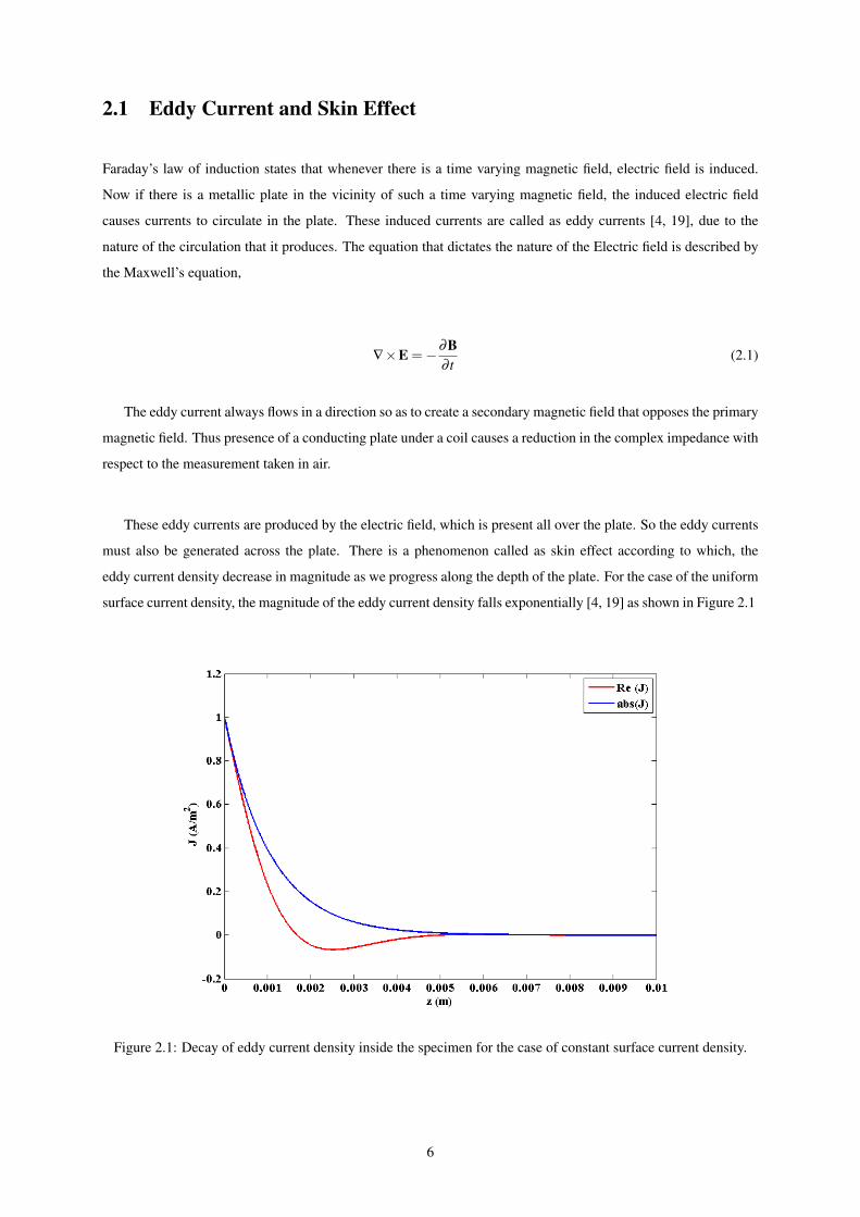
These eddy currents are produced by the electric field, which is present all over the plate. So the eddy currents
must also be generated across the plate. There is a phenomenon called as skin effect according to which, the
eddy current density decrease in magnitude as we progress along the depth of the plate. For the case of the uniform
surface current density, the magnitude of the eddy current density falls exponentially [4, 19] as shown in Figure 2.1
Figure 2.1: Decay of eddy current density inside the specimen for the case of constant surface current density.
6
2.2 Eddy Current Testing
The basic principles of ECT lies in the fact that the flow of secondary currents (eddy currents) in the presence of
defect and absence of a defect is different and thus producing different net magnetic field which can be picked up
by a sensor or observing the change in coil impedance.
There are different ways by which the eddy currents can be induced in a conductor.
1. Stationary conductor experiencing time varying magnetic field:
Conventional ECT utilizes the magnetic field that varies sinusoidally (by exciting the probe with a sinusoidal
current). If the time varying magnetic field is a short burst of pulse, it is called as Pulsed Eddy current testing.
The conventional ECT is based on the fact that a sinusoidal excitation causes a magnetic field that is a sinu-
soid (time varying field). Hence according to Maxwell-Faraday equation a non-zero time varying magnetic
field will produce an electric field, which in turn causes the flow of eddy currents.
∮∂ s
E ·dl =−∫
s
∂B∂ t·ds (2.2)
The principle of pulsed eddy current testing is that a pulse signal is an infinite sum of sinusoids of various
amplitudes and various frequencies (result of Fourier series expansion of a repeated pulse). So this tech-
nique is similar to the conventional ECT but with multiple frequencies. The advantage of this technique
is that presence of lower frequencies causes the eddy currents to penetrate deeper into the conductor and
thus detecting an anomaly at the subsurface, and presence of higher frequency causing it to detect surface
anomalies. Hence this technique can cover a wide range of crack positions.
2. Moving a permanent magnet across a conductor:
Equation 2.2 dictates that eddy currents could be induced in a conductor in the presence of a time varying
magnetic field or by setting a relative motion (v) between the conductor and a permanent magnet [17].
When a permanent magnet is moved across a conductor (or vice versa), it results in a force (F) acting on the
electrons (of charge q) which is called the Lorentz force.
F = q(v×B) (2.3)
The direction of the flow of the electrons is controlled by Lenz’s law. Ampere’s law states that, presence of
non-zero current causes the existence of a magnetic field. This magnetic field is always in the direction that
opposes the primary field (according to Lenz’s law).
Thus regions where there is no defect, the sensed magnetic field is more or less nullified. The regions close
to the defect where the eddy currents deviates from its circular path, it produces maximum net magnetic field.
7
In this thesis, conventional ECT has been followed by utilizing single frequency excitation. The reason is that
these methods are well documented both experimentally as well as theoretically. Also it is simpler to simulate the
experiments in commercially available finite element method based software.
2.3 Eddy Current Probes
The eddy current probes are classified by the mode of operation and configuration. The mode of operation usually
refers to the probe arrangement i.e. differential probe, absolute probe and reflection probe.
1. Differential Probe:
The differential probe has two coils wound in opposition. In the absence of a defect, both the coil pick up
the similar field (due to the positioning of the probes), but in opposite directions. So effectively they tend to
cancel, thus giving a nearly zero net detected magnetic field. When one of the probes crosses the defect a
differential magnetic field exists.
2. Absolute Probe:
The absolute probe consists of a single test coil. In this case the coil detects certain magnetic field at any
instant. Presence or absence of a defect can be detected by a change in the detected net magnetic field or
looking at the coil impedance plot. Presence of a defect increases the coil impedance due to the reduction of
the secondary magnetic field.
3. Reflection probe:
This type of probe arrangement is similar to the differential probe. But in this case, one of the two probes is
excited with the time varying current, and the other picks up the net magnetic field or the emf.
Based on the configuration, the probes are classified as,
1. Surface probe:
It’s an arrangement in which, the probe is located above the surface of the inspecting material. The inspecting
material is usually flat and the probe is placed above it. This is the case being used in this work.
2. Encircling probe:
It’s an arrangement in which, the probe encircles the specimen/material under test. The specimen is usually
a tubular structure. The probe can encircle in the OD (Outer Diameter) or the ID (Inner Diameter). The
inspection that uses ID encircling probe is called Remote Field Eddy Current Testing.
2.4 Measurements
The magnetic field carries the information of presence of defects. So in order to measure the magnetic fields, com-
mercially available magneto-resistive sensors like GMR (Giant Magneto-Resistance) [6, 10], AMR (Anisotropic
Magnetic Resistance) and Hall sensors are utilized. These sensors, transduces the magnetic field to a proportional
voltage. In this work GMR sensor has been utilized to detect the magnetic field. The reason for using GMR sensor
is that it has a high sensitivity with respect to AMR sensor and Hall effect sensor.
8

2.5 Parameters Affecting the Magnitude of Eddy Current Response
Eddy currents induced in the testing sample are important for the identification of any anomaly in the sample.
There are several factors that affect the density of eddy current that is induced in the sample. These factors are
broadly divided into two different parameters. They are coil parameters and sample parameters.
1. Coil Parameters:
The parameters of the coil that affect the distribution of eddy current density are,
(a) Coil geometry such as the cross section area of the coil and number of turns.
(b) Electrical parameters such as excitation current and excitation frequency (skin depth).
(c) Distance between the coil and the sample (lift off).
2. Sample Parameters:
The parameters of the sample that affect the distribution of eddy current density are,
(a) The sample thickness.
(b) The physical parameters of a sample such as the permittivity, permeability and conductivity.
The other factor that affect the magnitude of the eddy currents in the plate is the edge effect [11] . This happens
when the probe is close to the edge of the testing sample. So all the eddy current are forced to get concentrated
near the surface of the edge thus increasing the secondary magnetic field.
2.6 Potential Applications of ECT
Eddy current methods are employed in vast range of industries. The main reason for considering this method is
that it has very high sensitivity. It has the capability of detecting a very small defects provided they fall within the
range of one skin depth. These methods are also applied to quality control and in-service integrity inspection. The
eddy currents respond to parameters such as conductivity, magnetic permeability, excitation current and frequency,
geometry of the defect. Some of the specific advantages of ECT are as follows –
1. Measuring the thickness of conductive materials.
2. Location of buried metals.
2.7 Advantages of ECT
1. This method can be readily applied to test conductive materials.
2. The probe need not be in contact with the surface. It doesn’t need any surface preparation (such as ultrasonic
testing).
3. It is sensitive to large number of parameters such as conductivity, permeability, geometry (e.g. dimensions,
lift off, etc.)
9
2.8 Disadvantages of ECT
1. Results can be obtained only for electrically conducting materials.
2. The thickness of the samples usually range from 1 mm to 10 mm. (In this thesis we address this issue).
3. Analysis for ferromagnetic materials are difficult. The interpretation of the results are not easy as compared
to non ferromagnetic materials.
2.9 Formulation of the Dilation Parameters
The focus of this section is to formulate the electrical parameters [15] of the probe that need to be satisfied in order
that the principle of dilation invariance is satisfied. Let us assume that the dilation parameter to be k.
1. Frequency(ω):
In order to achieve the invariance of the magnetic field at any point along the depth of plate, the standard
depth of penetration (δ ) of the material has to be considered.
J ∝ e−zδ , (2.4)
where δ =
√2
jωµσ
Here µ and σ are the magnetic permeability and electrical conductivity of the sample. The standard depth
of penetration should be the same for both the cases (dilated and the non-dilated version). Since the sample
thickness is dilated, the skin depth also needs to be dilated. Let the dilated quantities be represented by
primes (’). So comparing the non-dilated and dilated version of the skin depth,
δ =
√2
jωµσ, δ
′ =
√2
jω ′µσ
Hence it is observed that for the skin depth to be dilated by k times, the frequency has to be dilated k−2 times
ω′ = k−2
ω (2.5)
This suggests that when the thickness of the plate is increased by k times, the excitation frequency has to be
reduced by k2 times. This relation is intuitively true because as the operation frequency decreases, the depth
of penetration of the eddy current increases, in other words the rate at which the magnitude of eddy current
diminishes along the depth is reduced i.e. it decreases at a slower rate.
2. Magnetomotive force (mm f ):
Magnetomotive force is analogous to electromotive force (em f ) in electrical circuits. The mm f depends on
the number of turns (N) present in the coil and the excitation current (I). The mm f is given by the relation,
mm f = NI (2.6)
10
The mm f has to be dilated k times. So the relation is,
mm f ′ = k ∗mm f
N′I′ = k ∗ (NI)
So from this equation it is clear that either N or I can be dilated by k times. If one of them is dilated,
the other component is to be kept an invariant. It is possible to dilate I retaining N as an invariant, but on
dilation the coil cross section area increases by k2. So, the number of turns needs to be increased in order to
accommodate this. Hence it is better to dilate N retaining I as an invariant. It is also possible to dilate both
N and I, such that their product (mm f ) is dilated by k times.
A detailed proof of the Invariance of the magnetic field upon dilation of the dimensional and electrical param-
eters is described in Chapter 6.
11

12
Chapter 3
Simulation of the study
The problems involving eddy currents can be verified by simulating them using a numerical simulation program.
For an isotropic, non-magnetic medium, the field equation (that needs to be solved) can be represented using the
Magnetic Vector Potential (A) as,
∇2A+ jωµσA = µJs (3.1)
This is the differential equation when we are using low frequency (ω) excitation (few kHz). Here µ and σ
are the magnetic permeability and electrical conductivity respectively which is a scalar (isotropic medium). The
source current density is represented by Js. The solution to such problems doesn’t exists in a closed form manner
(will be shown in the theoretical section for an axially symmetric model without a crack). So to solve such a
system, the finite element method is used. Softwares like Comsol, performs solution to these problems, based on
the geometry of the problem assigned to it by the user. In this case, the geometry is a plate of specific dimension,
with a crack and a probe of specific dimension.
Usually in problems involving finite element methods, a boundary has to be specified, which is situated at a
very large distance, so that the boundary condition of the variable that is being solved is 0.
It is also interesting to know that, the reduced version of a 3-d model can also be made, by considering sym-
metry along one of the rotation axis (2-d axi-symmetric model). The advantage is that the numerical noise is much
reduced. However, here since the plate is in the shape of a cuboid, this reduction of axis is not possible, and thus
following the 3-d model.
3.1 Advantages of Simulation
The main advantage of simulation is that the electromagnetic quantities such as the electric field, current density,
magnetic field and coil impedance can be determined from the magnetic vector potential. Since the entire domain
has been solved, we can obtain the value from any point within the domain. Some of the other advantages of
simulation are,
13

1. The material that is considered can be assumed to have the properties as desired. In this case, isotropic and
non-magnetic.
2. It is easy to find the values of variables in inaccessible areas (such as inside the plate).
3. Assumption such as presence or absence of external magnetic field (if necessary) and current density (i.e. a
coil) can be applied.
3.2 Disadvantages of Simulation
Even though simulation seems to be quite good for certain kinds of problems, it has its own disadvantages. They
are,
1. It is difficult to incorporate the properties of ferromagnetic materials.
2. The solutions are obtained by triangulation of the regions, which may induce small errors to the obtained
solution. This in an iterative process, it might get amplified.
3. Based on the convergence method, the time taken can be very long.
3.3 Dimensional and Electrical Specifications
This simulation is the replica of the experimental study. So the geometrical and electrical parameters of the plate,
crack and the probe for both the cases are followed from the experimental studies.The geometry of the problem
can be seen in Figure 3.1, which is simulated in Comsol.
Figure 3.1: Geometry of the ECT implemented in Comsol.
The various components of the problem such as the probe, air region and plate are meshed and is shown in the
Appendix C.
14

3.4 Simulation Measures and Considerations
As said before, the finite element based simulation can lead to the presence of noise with the required signal. In
order to minimize the noise and obtain the best possible result, certain measures are to be followed.
1. The air boundary should be placed at a sufficiently large distance from the geometries, so that the magnetic
vector potential A is very low and thus can be assumed to be 0 (Dirichlet boundary condition). Usually for
these cases, the boundaries are specified to be at least twice the geometry of the plate with the probe and
plate positioned in the center of the air box. The height should be at least twice the height of probe and the
plate. The magnetic vector potential decays faster in air as compared to conducting material, so it’s sufficient
to take the above mentioned quantity as boundary.
2. Meshing of the region was made as uniform as possible by selecting appropriate minimum size of the mesh
and the growth rate. Uniform and high density mesh creates more resolution to the system for the evaluation
of Magnetic vector potential. However, there is a tradeoff i.e. maximizing the density of the meshes propa-
gates error. So the mesh settings have to be changed for every simulation test and thus choose the one that
yields the best result.
3. The probe, being cylindrical, should have a low curvature resolution in order to closely approximate the
curvature to a circle.
4. The air region surrounding the lift off region is very narrow, and the air region away from the probe is large.
The solution would be to consider a small mesh size for that region and a large mesh element for the other
air regions with a nominal mesh growth rate. However, this type of meshing causes inverted mesh elements,
and thus approximating linear meshes at some regions (so the second order solutions are computed as first
order solutions). This is reflected in the obtained results as huge noise being non-linearly superimposed with
the required signal.
5. In order to address the problem of inverted mesh elements during meshing, the region with small air gap was
meshed separately by adding a separate region (which is defined with the properties of air and is called as
high density mesh region as shown in Figure 3.2). This region was meshed separately apart from the others.
This region was given a small mesh element size and small growth rate and also since the solution varies at
a higher rate in that region, adaptive mesh refinement (AMR) technique was used. This splits the longest
side of a mesh thus forming sub-meshes. This is useful in the case where the solutions change at a faster
rate compared to mesh element size. Applying these techniques, increases the computation time but with a
payoff that the results are more smooth and low errors
6. There might be some noise superimposed with the signal. In order to smooth them, the noisy signal has
to be linearly convolved with an N-point Gaussian. This is same as low pass filtering of the noisy signal
which smoothens the high frequency (fast varying) components associated with the signal. The size (N) of
the Gaussian and its variance depends on the level of smoothening required. High variance causes, some of
the essential components being smoothened. So a variance of 1 to 2 can be selected.
15
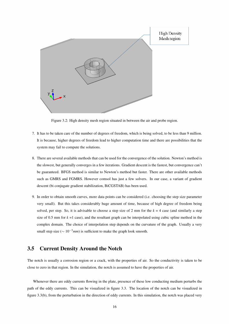
Figure 3.2: High density mesh region situated in between the air and probe region.
7. It has to be taken care of the number of degrees of freedom, which is being solved, to be less than 9 million.
It is because, higher degrees of freedom lead to higher computation time and there are possibilities that the
system may fail to compute the solutions.
8. There are several available methods that can be used for the convergence of the solution. Newton’s method is
the slowest, but generally converges in a few iterations. Gradient descent is the fastest, but convergence can’t
be guaranteed. BFGS method is similar to Newton’s method but faster. There are other available methods
such as GMRS and FGMRS. However comsol has just a few solvers. In our case, a variant of gradient
descent (bi conjugate gradient stabilization, BiCGSTAB) has been used.
9. In order to obtain smooth curves, more data points can be considered (i.e. choosing the step size parameter
very small). But this takes considerably huge amount of time, because of high degree of freedom being
solved, per step. So, it is advisable to choose a step size of 2 mm for the k = 4 case (and similarly a step
size of 0.5 mm for k =1 case), and the resultant graph can be interpolated using cubic spline method in the
complex domain. The choice of interpolation step depends on the curvature of the graph. Usually a very
small step size (∼ 10−3mm) is sufficient to make the graph look smooth.
3.5 Current Density Around the Notch
The notch is usually a corrosion region or a crack, with the properties of air. So the conductivity is taken to be
close to zero in that region. In the simulation, the notch is assumed to have the properties of air.
Whenever there are eddy currents flowing in the plate, presence of these low conducting medium perturbs the
path of the eddy currents. This can be visualized in figure 3.3. The location of the notch can be visualized in
figure 3.3(b), from the perturbation in the direction of eddy currents. In this simulation, the notch was placed very
16
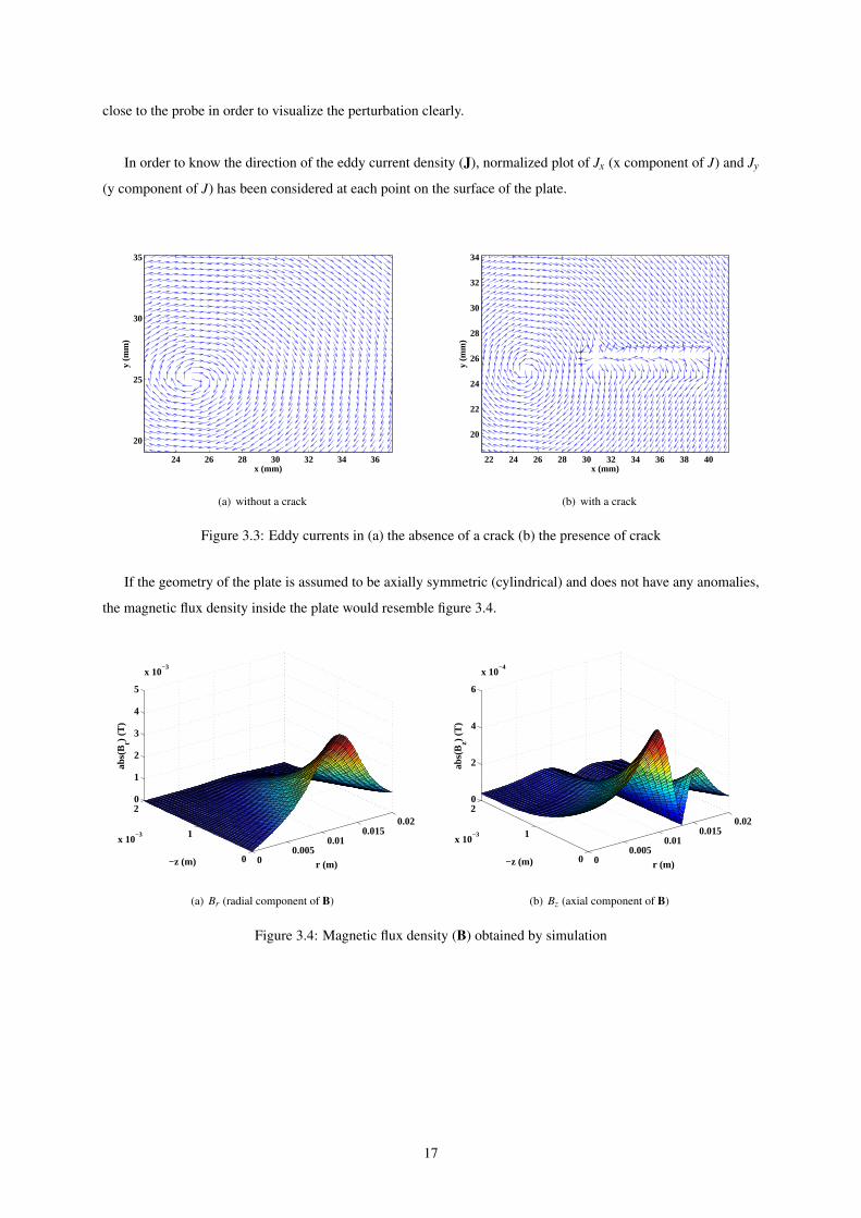
close to the probe in order to visualize the perturbation clearly.
In order to know the direction of the eddy current density (J), normalized plot of Jx (x component of J) and Jy
(y component of J) has been considered at each point on the surface of the plate.
24 26 28 30 32 34 36
20
25
30
35
x (mm)
y (m
m)
(a) without a crack
22 24 26 28 30 32 34 36 38 40
20
22
24
26
28
30
32
34
x (mm)y
(mm
)
(b) with a crack
Figure 3.3: Eddy currents in (a) the absence of a crack (b) the presence of crack
If the geometry of the plate is assumed to be axially symmetric (cylindrical) and does not have any anomalies,
the magnetic flux density inside the plate would resemble figure 3.4.
00.005
0.010.015
0.02
0
1
2
x 10−3
0
1
2
3
4
5
x 10−3
r (m)−z (m)
abs(
B r) (T
)
(a) Br (radial component of B)
00.005
0.010.015
0.02
0
1
2
x 10−3
0
2
4
6
x 10−4
r (m)−z (m)
abs(
B z) (T
)
(b) Bz (axial component of B)
Figure 3.4: Magnetic flux density (B) obtained by simulation
17

18
Chapter 4
Experimentation of the Study
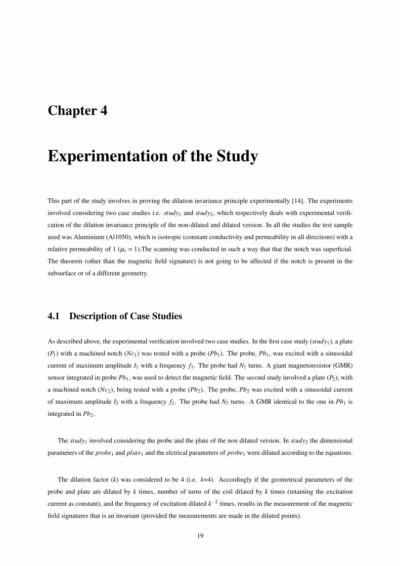
This part of the study involves in proving the dilation invariance principle experimentally [14]. The experiments
involved considering two case studies i.e. study1 and study2, which respectively deals with experimental verifi-
cation of the dilation invariance principle of the non-dilated and dilated version. In all the studies the test sample
used was Aluminium (Al1050), which is isotropic (constant conductivity and permeability in all directions) with a
relative permeability of 1 (µr = 1).The scanning was conducted in such a way that that the notch was superficial.
The theorem (other than the magnetic field signature) is not going to be affected if the notch is present in the
subsurface or of a different geometry.
4.1 Description of Case Studies
As described above, the experimental verification involved two case studies. In the first case study (study1), a plate
(P1) with a machined notch (Nc1) was tested with a probe (Pb1). The probe, Pb1, was excited with a sinusoidal
current of maximum amplitude I1 with a frequency f1. The probe had N1 turns. A giant magnetoresistor (GMR)
sensor integrated in probe Pb1, was used to detect the magnetic field. The second study involved a plate (P2), with
a machined notch (Nc2), being tested with a probe (Pb2). The probe, Pb2 was excited with a sinusoidal current
of maximum amplitude I2 with a frequency f2. The probe had N2 turns. A GMR identical to the one in Pb1 is
integrated in Pb2.
The study1 involved considering the probe and the plate of the non dilated version. In study2 the dimensional
parameters of the probe1 and plate1 and the elctrical parameters of probe1 were dilated according to the equations.
The dilation factor (k) was considered to be 4 (i.e. k=4). Accordingly if the geometrical parameters of the
probe and plate are dilated by k times, number of turns of the coil dilated by k times (retaining the excitation
current as constant), and the frequency of excitation dilated k−2 times, results in the measurement of the magnetic
field signatures that is an invariant (provided the measurements are made in the dilated points).
19
4.2 Dimension and Electrical Specification of the Probe, Plate and the
Crack
Study1 constituted a machined notch of dimensions 0.5×12×0.5 mm3 (W1×L1×T1 ) in the Aluminum plate P1.
The thickness of the plate (P1) was 1 mm. The probe had a cylindrical geometry with a rectangular cross section of
area 45mm2.The excitation current for the probe was I1=50 mA. The excitation frequency used was 10 kHz. The
reason for choosing this value is that, since the notch is present on the top surface and exists till 0.5 mm below, and
the skin depth should be atleast close to this distance. Hence on knowing the conductivity, the frequency f1 was
calculated.
The parameters for both the case studies are specified in Table 4.2 and Table 4.2. In study2 the crack width
was not dilated, as because most of the eddy currents flow is perpendicular to the notch length, the effect of eddy
current perturbation due to the width, is very less.
Table 4.1: Geometrical Specification for study1 and study2
Dimensional Parameters study1 (k = 1) study2 (k = 4)Notch dimension (W ×L×T ) 0.5×12.5×0.5mm3 0.5×50×2mm3
Thickness of the specimen 1 mm 4 mmProbe - Inner Diameter (ID) 10 mm 40 mmProbe - Cross Section Area 45 mm2 720 mm2
Probe - Height 9 mm 36 mm
Table 4.2: Electrical Specification for study1 and study2
Electrical Parameters study1 (k = 1) study2 (k = 4)Number of turns in probe (N) 130 520
Current amplitude (I) 50 mA 50 mAExcitation frequency (( f )) 10 kHz 625 Hz
4.3 Experimental Setup
The experimental setup used for the experiments is depicted in figure 4.1. It includes a Fluke 5700 calibrator work-
ing as an A.C. current source, a USB DAQ for signal acquisition, and a XY positioning system. The instruments
are remotely controlled using an application developed in MATLAB and installed in a desktop PC that communi-
cates with the instruments through RS232 (XY scanner), GPIB (Fluke 5700) and USB (NI USB DAQ 6251).
The current applied to the excitation coil of the probe is produced by the calibrator functioning as a current
generator. The voltage signal obtained from the GMR (VGMR) is amplified by a low noise instrumentation amplifier
stage that was implemented using an INA118 with a gain value set to 101. The output signal is applied to the
analogue inputs of the 16-bits multifunction board working with a maximum acquisition rate of 1.2 MHz. The
number of samples per position was fixed to 8000 (for 100 periods). So depending on the excitation frequency, the
20
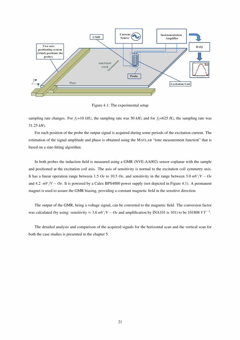
Figure 4.1: The experimental setup
sampling rate changes. For f1=10 kHz, the sampling rate was 50 kHz and for f2=625 Hz, the sampling rate was
31.25 kHz.
For each position of the probe the output signal is acquired during some periods of the excitation current. The
estimation of the signal amplitude and phase is obtained using the MATLAB “tone measurement function” that is
based on a sine-fitting algorithm.
In both probes the induction field is measured using a GMR (NVE-AA002) sensor coplanar with the sample
and positioned at the excitation coil axis. The axis of sensitivity is normal to the excitation coil symmetry axis.
It has a linear operation range between 1.5 Oe to 10.5 Oe, and sensitivity in the range between 3.0 mV/V −Oe
and 4.2 mV/V −Oe. It is powered by a Calex BPS4000 power supply (not depicted in Figure 4.1). A permanent
magnet is used to assure the GMR biasing, providing a constant magnetic field in the sensitive direction.
The output of the GMR, being a voltage signal, can be converted to the magnetic field. The conversion factor
was calculated (by using: sensitivity ≈ 3.6 mV/V −Oe and amplification by INA101 is 101) to be 101808 V T−1.
The detailed analysis and comparison of the acquired signals for the horizontal scan and the vertical scan for
both the case studies is presented in the chapter 5.
21

22
Chapter 5
Discussion
In this chapter, we are going to compare the experimental and simulation results for the two case studies (study1
and study2) which was introduced in chapter 4 . Two different scans were performed for each of the case studies.
They are horizontal scan and the vertical scan which is described in the following section. Each of the section
is assigned to describe the results obtained and compare the magnetic field signature (for each scan) between the
case study 1 and case study 2. We will also investigate the discrepancy in the comparison of the magnetic field
signatures between the case study 1 and case study 2.
5.1 Results from Experiment
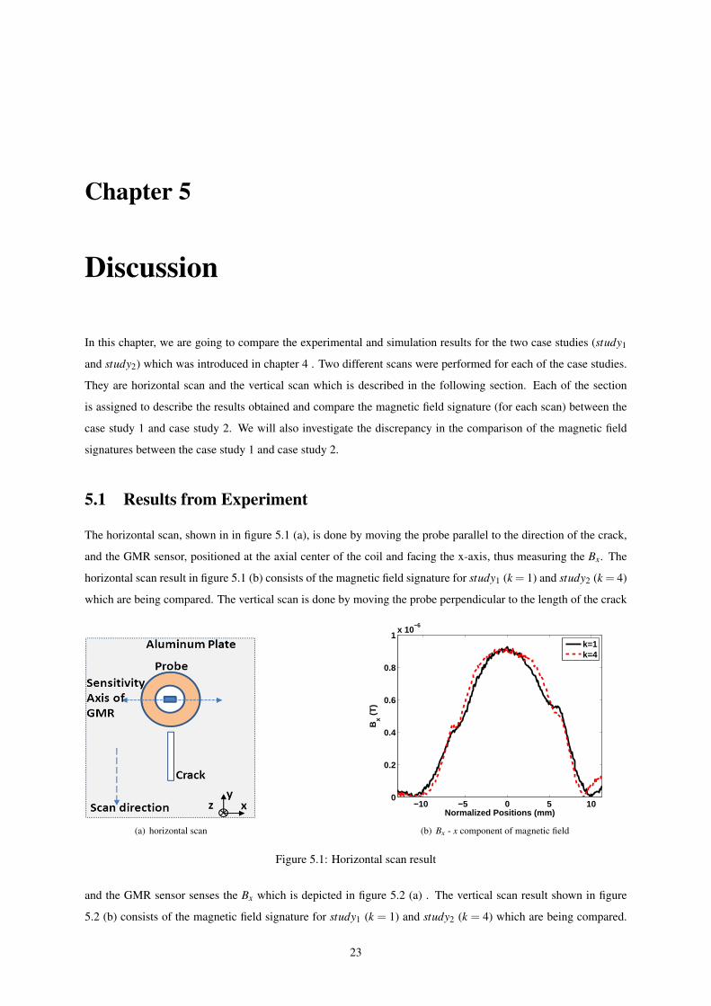
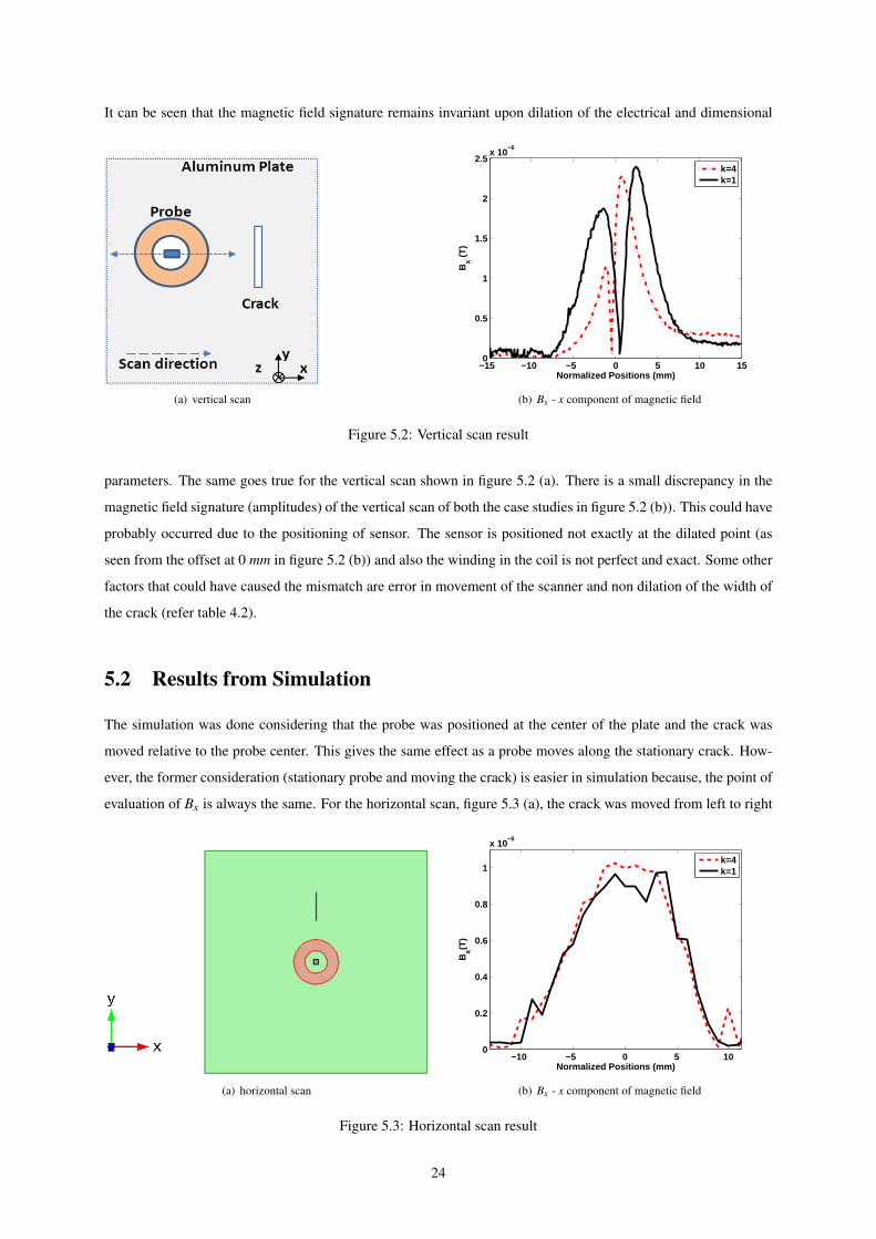
The horizontal scan, shown in in figure 5.1 (a), is done by moving the probe parallel to the direction of the crack,
and the GMR sensor, positioned at the axial center of the coil and facing the x-axis, thus measuring the Bx. The
horizontal scan result in figure 5.1 (b) consists of the magnetic field signature for study1 (k = 1) and study2 (k = 4)
which are being compared. The vertical scan is done by moving the probe perpendicular to the length of the crack
(a) horizontal scan
−10 −5 0 5 100
0.2
0.4
0.6
0.8
1x 10
−6
Normalized Positions (mm)
Bx (
T)
k=1k=4
(b) Bx - x component of magnetic field
Figure 5.1: Horizontal scan result
and the GMR sensor senses the Bx which is depicted in figure 5.2 (a) . The vertical scan result shown in figure
5.2 (b) consists of the magnetic field signature for study1 (k = 1) and study2 (k = 4) which are being compared.
23
It can be seen that the magnetic field signature remains invariant upon dilation of the electrical and dimensional
(a) vertical scan
−15 −10 −5 0 5 10 150
0.5
1
1.5
2
2.5x 10
−6
Normalized Positions (mm)
Bx (
T)
k=4k=1
(b) Bx - x component of magnetic field
Figure 5.2: Vertical scan result
parameters. The same goes true for the vertical scan shown in figure 5.2 (a). There is a small discrepancy in the
magnetic field signature (amplitudes) of the vertical scan of both the case studies in figure 5.2 (b)). This could have
probably occurred due to the positioning of sensor. The sensor is positioned not exactly at the dilated point (as
seen from the offset at 0 mm in figure 5.2 (b)) and also the winding in the coil is not perfect and exact. Some other
factors that could have caused the mismatch are error in movement of the scanner and non dilation of the width of
the crack (refer table 4.2).
5.2 Results from Simulation
The simulation was done considering that the probe was positioned at the center of the plate and the crack was
moved relative to the probe center. This gives the same effect as a probe moves along the stationary crack. How-
ever, the former consideration (stationary probe and moving the crack) is easier in simulation because, the point of
evaluation of Bx is always the same. For the horizontal scan, figure 5.3 (a), the crack was moved from left to right
(a) horizontal scan
−10 −5 0 5 100
0.2
0.4
0.6
0.8
1
x 10−6
Bx(T
)
Normalized Positions (mm)
k=4k=1
(b) Bx - x component of magnetic field
Figure 5.3: Horizontal scan result
24
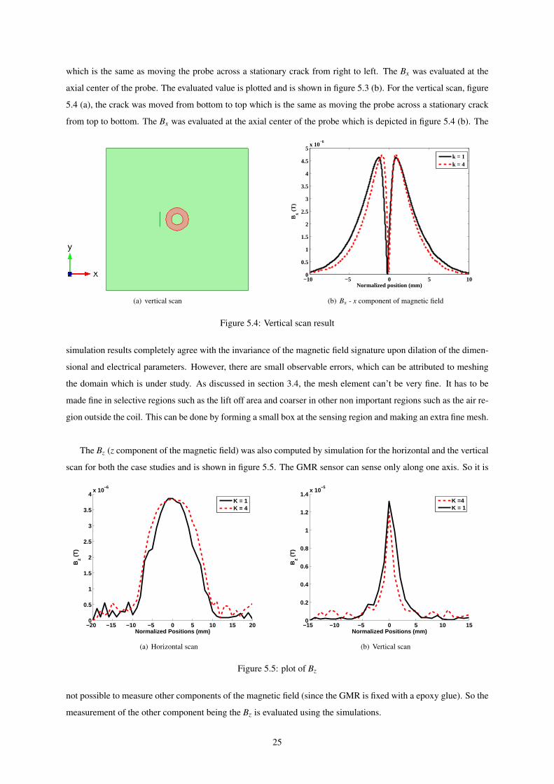
which is the same as moving the probe across a stationary crack from right to left. The Bx was evaluated at the
axial center of the probe. The evaluated value is plotted and is shown in figure 5.3 (b). For the vertical scan, figure
5.4 (a), the crack was moved from bottom to top which is the same as moving the probe across a stationary crack
from top to bottom. The Bx was evaluated at the axial center of the probe which is depicted in figure 5.4 (b). The
(a) vertical scan
−10 −5 0 5 100
0.5
1
1.5
2
2.5
3
3.5
4
4.5
5x 10
−6
Normalized position (mm)B
x (T
)
k = 1k = 4
(b) Bx - x component of magnetic field
Figure 5.4: Vertical scan result
simulation results completely agree with the invariance of the magnetic field signature upon dilation of the dimen-
sional and electrical parameters. However, there are small observable errors, which can be attributed to meshing
the domain which is under study. As discussed in section 3.4, the mesh element can’t be very fine. It has to be
made fine in selective regions such as the lift off area and coarser in other non important regions such as the air re-
gion outside the coil. This can be done by forming a small box at the sensing region and making an extra fine mesh.
The Bz (z component of the magnetic field) was also computed by simulation for the horizontal and the vertical
scan for both the case studies and is shown in figure 5.5. The GMR sensor can sense only along one axis. So it is
−20 −15 −10 −5 0 5 10 15 200
0.5
1
1.5
2
2.5
3
3.5
4x 10
−6
Normalized Positions (mm)
Bz (
T)
K = 1K = 4
(a) Horizontal scan
−15 −10 −5 0 5 10 150
0.2
0.4
0.6
0.8
1
1.2
1.4x 10
−5
Normalized Positions (mm)
Bz (
T)
K =4K = 1
(b) Vertical scan
Figure 5.5: plot of Bz
not possible to measure other components of the magnetic field (since the GMR is fixed with a epoxy glue). So the
measurement of the other component being the Bz is evaluated using the simulations.
25

26
Chapter 6
Analytical Verification to Dilation
Invariance Problem
In this chapter we derive the required field equation in differential form, using the Maxwell’s equation and then
solve analytically the differential equation at various regions by obeying certain boundary conditions. In the
first section, the field equation is arrived using the current sheet approximation for the coil. This is followed by
deriving the solution of the field equation and then computing the magnetic flux density. This is followed by the
section where the invariance of magnetic flux density is proved upon the dilation of the dimensional and electrical
parameters.
6.1 Field Equation
The differential form of the Maxwell’s equations [4, 19], which is required to derive the field equations, are shown
here.
∇×E = −∂B∂ t
(6.1)
∇×H = J+∂D∂ t
(6.2)
∇ ·B = 0 (6.3)
∇ ·D = ρ (6.4)
where B is the magnetic flux density vector, E is the electric field intensity vector, D is the electric displacement
field, J is the current density vector (which is the sum of source current density and eddy current density) and ρ is
the free electric charge density.
Equation 6.3 which is called the Gauss law for magnetism, states the net magnetic flux density (magnetic field)
doesn’t diverge. Hence it must form a purely rotational vector. Helmholtz decomposition of the magnetic field
27
yields 2 components, one irrotational (divergent field) and the other solenoidal (rotational field).
B = ∇φ +∇×A (6.5)
Substituting equation 6.5 in equation 6.3, we have
∇ ·B = ∆φ +∇ · (∇×A) (6.6)
But the divergence of the curl is 0 and the left hand side of equation 6.6 is 0. Which implies that the Laplacian
of the potential (∆φ) is 0. So the ∇φ can be taken to be 0. Thus substituting this information in equation 6.5, we
finally obtain
B = ∇×A (6.7)
Here A is the magnetic vector potential (MVP) [5]. The main advantage of using MVP to formulate the field
equation is, since A is orthogonal to B, it is always oriented along the electric field (which can be deduced by
substituting equation 6.5 in equation 6.1.
The problem under study actually consists of a defect in the conductor. In order to simplify the whole structure,
we can consider the case of absence of cracks and the plates are semi-infinite (conductive half space).Since the coil
has a cylindrical geometry, it is possible to assume that it has a rectangular cross section. In order to formulate the
field equation for this kind of problem, the idea of a current sheet approximation to the coil can be used [5, 21].
6.2 Formulation of the Field Equation
In the previous section 6.1, we had assumed a rectangular geometry for the cross section of the coil. So we can
say that the coil has an axially symmetric geometry (coil has a cylindrical structure, with the cross section being a
rectangle).
So we can assume (as an approximation) that the coil is built up of many loops of current (with each loop
carrying a current I). These current loops are perpendicular to the sheet in a given plane [21] (along the cross
section of the coil). This is depicted in figure 6.1
In order to arrive at the field field equation, we need to consider the differential form of Maxwell-Ampere’s
law (equation 6.2),
∇×H = Js +σE + ε∂E∂ t
(6.8)
where H is the intensity of the magnetic field and Js is the source current density. The displacement current density
28
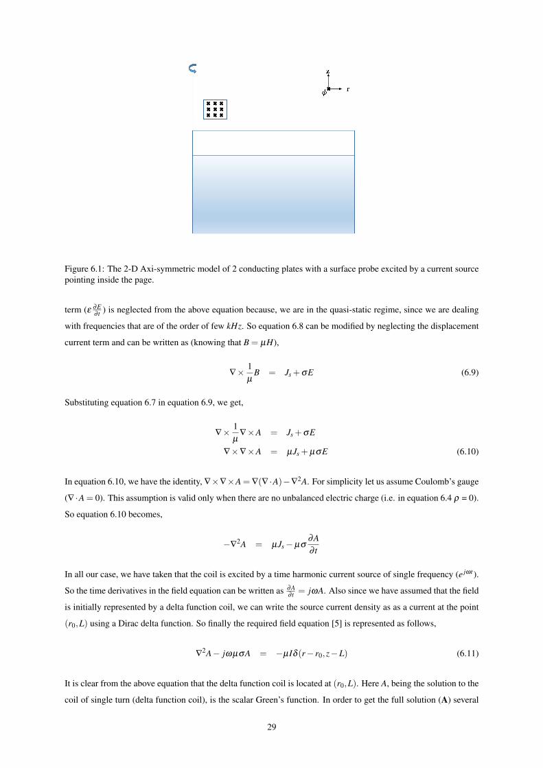
Figure 6.1: The 2-D Axi-symmetric model of 2 conducting plates with a surface probe excited by a current sourcepointing inside the page.
term (ε ∂E∂ t ) is neglected from the above equation because, we are in the quasi-static regime, since we are dealing
with frequencies that are of the order of few kHz. So equation 6.8 can be modified by neglecting the displacement
current term and can be written as (knowing that B = µH),
∇× 1µ
B = Js +σE (6.9)
Substituting equation 6.7 in equation 6.9, we get,
∇× 1µ
∇×A = Js +σE
∇×∇×A = µJs +µσE (6.10)
In equation 6.10, we have the identity, ∇×∇×A = ∇(∇ ·A)−∇2A. For simplicity let us assume Coulomb’s gauge
(∇ ·A = 0). This assumption is valid only when there are no unbalanced electric charge (i.e. in equation 6.4 ρ = 0).
So equation 6.10 becomes,
−∇2A = µJs−µσ
∂A∂ t
In all our case, we have taken that the coil is excited by a time harmonic current source of single frequency (e jωt ).
So the time derivatives in the field equation can be written as ∂A∂ t = jωA. Also since we have assumed that the field
is initially represented by a delta function coil, we can write the source current density as as a current at the point
(r0,L) using a Dirac delta function. So finally the required field equation [5] is represented as follows,
∇2A− jωµσA = −µIδ (r− r0,z−L) (6.11)
It is clear from the above equation that the delta function coil is located at (r0,L). Here A, being the solution to the
coil of single turn (delta function coil), is the scalar Green’s function. In order to get the full solution (A) several
29
delta function coils of required number of turns is linearly superposed (integrated because of the continuous case)
along the region in which the cross section of the coil is defined. The delta function coil above the conducting
plates is shown in figure 6.2
The consideration of the axially symmetric geometry to the probe-sample problem, reduces the problem of the
field equation that needs to be evaluated only for the φ (azimuthal) component of the MVP (because in axisym-
metric model we can assume the electric field to be pointing inside the page and thus the MVP pointing outside the
page or vice-versa and hence the MVP has only one component). So equation 6.11 can be rewritten in cylindrical
co-ordinate as,
∇2Aφ (r,φ ,z)− jωµσAφ (r,φ ,z) = 0 (6.12)
In the above equation, it can be noted that the source current term is not present. This euqation is valid at
every point in space except at (r0,L), where the source current density term could be included while solving the
differential equation and using the boundary conditions.
Equation 6.12 is called the Helmholtz equation. Expanding the azimuthal (φ ) component of the vector Lapla-
cian and substituting it in equation 6.12 we have
∂ 2Aφ
∂ r2 +1r2
∂ 2Aφ
∂φ 2 +∂ 2Aφ
∂ z2 +1r
∂Aφ
∂ r+
2r2
∂Aφ
∂φ−
Aφ
r2 − jωµσAφ = 0 (6.13)
Equation 6.13 is the differential equation that governs the variation of the MVP in the space (r,z), which needs
to be solved analytically. It is also possible to note the advantage of considering solving for A over B. B is or-
thogonal to A. So it has 2 components in the plane which needs to be accounted for, they are Br(r,z) and Bz(r,z).
Thus the field equation becomes coupled and the solution for it is almost impossible to solve, involving 4 different
variables at any point in the 2D space.
Equation 6.13 doesn’t explicitly deal with excitation source. This can be incorporated into the equation while
solving the partial differential equation considering the boundary conditions at the location of the delta function
coil. First, compute the Green’s function for the filamentary current loop (delta function coil, DFC) and then apply
superposition theorem to compute the total magnetic vector potential for the thick coil. The main advantage of ap-
plying this theorem to the problem is that, it becomes easier to compute the regions for the boundary and existence
of continuity of variables along the boundary.
6.3 Solution for the Field Equation
The geometry of the problem, for which the field equation has to be analysed, consists of two conducting plates,
stacked one above the other. As described in the previous section, the geometry has been assumed to be cylindri-
cally symmetric. The radius of the plate is assumed to be infinite and thickness of the first plate is C . The second
30
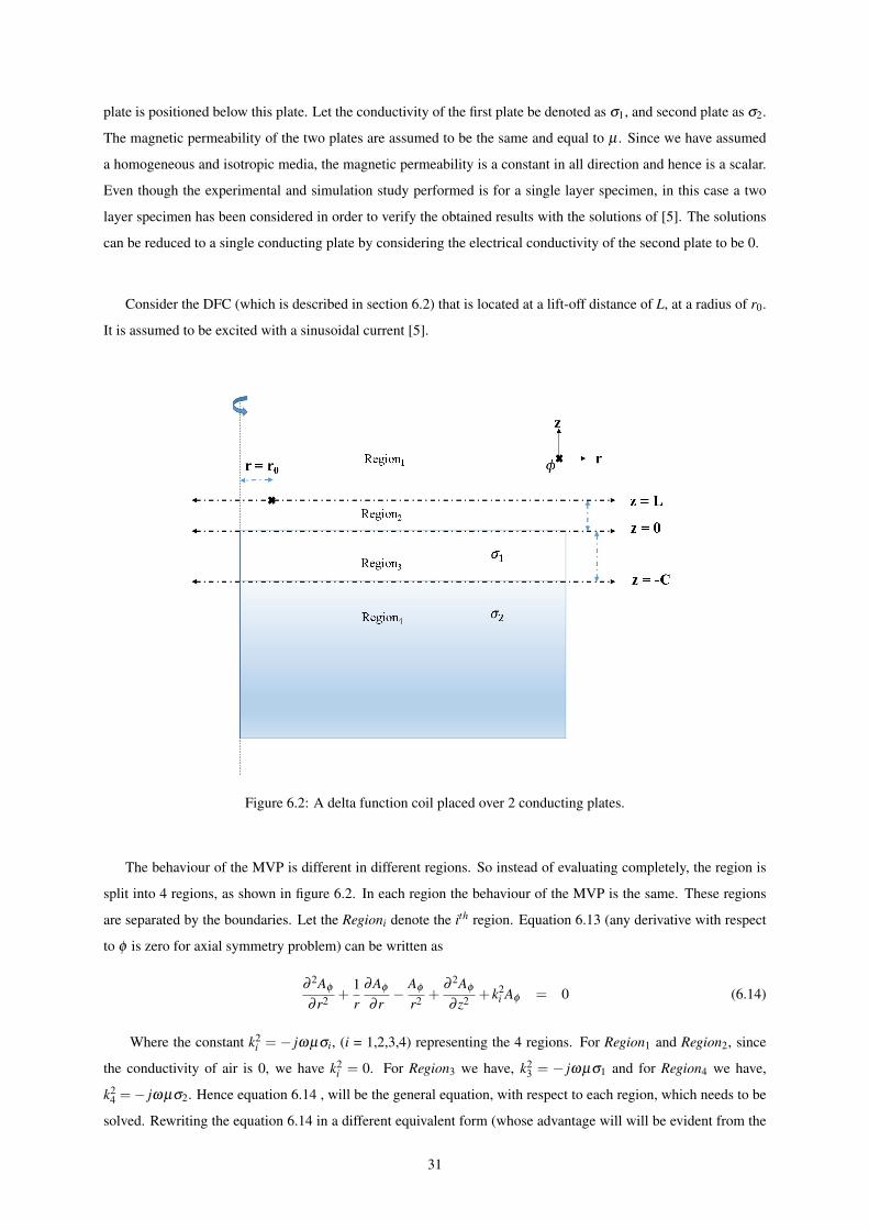
plate is positioned below this plate. Let the conductivity of the first plate be denoted as σ1, and second plate as σ2.
The magnetic permeability of the two plates are assumed to be the same and equal to µ . Since we have assumed
a homogeneous and isotropic media, the magnetic permeability is a constant in all direction and hence is a scalar.
Even though the experimental and simulation study performed is for a single layer specimen, in this case a two
layer specimen has been considered in order to verify the obtained results with the solutions of [5]. The solutions
can be reduced to a single conducting plate by considering the electrical conductivity of the second plate to be 0.
Consider the DFC (which is described in section 6.2) that is located at a lift-off distance of L, at a radius of r0.
It is assumed to be excited with a sinusoidal current [5].
Figure 6.2: A delta function coil placed over 2 conducting plates.
The behaviour of the MVP is different in different regions. So instead of evaluating completely, the region is
split into 4 regions, as shown in figure 6.2. In each region the behaviour of the MVP is the same. These regions
are separated by the boundaries. Let the Regioni denote the ith region. Equation 6.13 (any derivative with respect
to φ is zero for axial symmetry problem) can be written as
∂ 2Aφ
∂ r2 +1r
∂Aφ
∂ r−
Aφ
r2 +∂ 2Aφ
∂ z2 + k2i Aφ = 0 (6.14)
Where the constant k2i = − jωµσi, (i = 1,2,3,4) representing the 4 regions. For Region1 and Region2, since
the conductivity of air is 0, we have k2i = 0. For Region3 we have, k2
3 = − jωµσ1 and for Region4 we have,
k24 =− jωµσ2. Hence equation 6.14 , will be the general equation, with respect to each region, which needs to be
solved. Rewriting the equation 6.14 in a different equivalent form (whose advantage will will be evident from the
31

following equations), we get
(1r
∂
∂ rr
∂
∂ r− 1
r2
)Aφ +
∂ 2Aφ
∂ z2 + k2i Aφ = 0 (6.15)
Observing equation 6.15, we can readily come to know that the radial dependence of the MVP follows a Bessel
differential equation of first order. So in order to evaluate the above differential equation, we compute the First
order Hankel transform of the equation 6.15.
The Hankel transform is given by
H [ f (x)] =∫
∞
0x f (x)J1(sx)dx
= F(s)
Also Hankel transform of the sums is the sum of the individual Hankel transform.
H [ f (x)+g(x)] = H [ f (x)]+H [g(x)]
Computing the Hankel transform of the equation 6.15 and applying the aforementioned property and denoting
H[Aφ (r,z))
]= Ψφ (s,z)
H
[(1r
∂
∂ rr
∂
∂ r− 1
r2
)Aφ +
∂ 2Aφ
∂ z2 + k2i Aφ
]= 0
H
[(1r
∂
∂ rr
∂
∂ r− 1
r2
)Aφ
]+H
[∂ 2Aφ
∂ z2
]+H
[k2
i Aφ
]= 0
−s2Ψφ +
∂ 2Ψφ
∂ z2 + k2i Ψφ = 0
∂ 2Ψφ
∂ z2 −(s2− k2
i)
Ψφ = 0 (6.16)
This is a second order homogeneous linear differential equation in z. The general solution of equation 6.16 is
given by
Ψφ (s,z) = x(s)e−siz + y(s)esiz (6.17)
Where si =√
s2− k2i has been used for convenience. Equation 6.17 is the general structure of the MVP in the
Hankel domain. Writing the equation for individual regions,
Region1:
In this region z ∈ [L,∞). Also as z→ ∞, we have Ψφ → ∞. This is not true, because it violates energy
conservation. So in this region we take y(s) = 0. Thus the MVP reduces exponentially. The desired equation in
this region is given by,
Ψ1φ (s,z) = x1(s)e−s1z (6.18)
32
(Here, the superscripts represent the specific region.)
Region2:
In this region z ∈ [0,L]. The desired equation in this region is given by,
Ψ2φ (s,z) = x2(s)e−s2z + y2(s)es2z (6.19)
Region3:
In this region z ∈ [−C,0]. The desired equation in this region is given by,
Ψ3φ (s,z) = x3(s)e−s3z + y3(s)es3z (6.20)
Region4:
In this region z ∈ (−∞,−C].Also as z→ −∞, we have Ψφ → ∞. This is not true, because it violates en-
ergy conservation. So in this region we take x(s) = 0. Thus the MVP reduces exponentially. The desired equation
in this region is given by,
Ψ4φ (s,z) = y4(s)es4z (6.21)
Thus combining the field equations for various regions, we have
Region1 : Ψ1φ (s,z) = x1(s)e−s1z
Region2 : Ψ2φ (s,z) = x2(s)e−s2z + y2(s)es2z
Region3 : Ψ3φ (s,z) = x3(s)e−s3z + y3(s)es3z
Region4 : Ψ4φ (s,z) = y4(s)es4z
From the above equations, it is clear that there are 6 unknowns (x1(s), x2(s), y2(s), x3(s), y3(s), y4(s)), which
are to be accounted in order to get the solution for the MVP. So we need 6 different boundary conditions, to account
for 6 different unknowns. But we have only 3 boundaries (i.e. intersection of 2 regions).
Hence at each boundary we need 2 different conditions, so that we have 2 equations at each boundary. This can
be achieved by analysing the continuity of the magnetic vector potential and the magnetic field at the boundary.
The tangential component of the electric field is known to be continuous at the boundary. So this implies that the
magnetic vector potential is also continuous. Hence the boundary that separates the regions, will have the magnetic
vector potential that is essentially the same.
If we resolve the magnetic flux density vector into its tangential (horizontal) and vertical components, we can
apply the magnetic boundary condition and say that, there is a continuity in the vertical component and that the
horizontal component of the magnetic flux density is discontinuous, which arises due to the discontinuity in the
magnetic permeability.
33
So from this information, we have that the horizontal component (radial component in our case) of the magnetic
field is discontinuous at the boundary. In order to resolve the components of the magnetic field from the magnetic
vector potential, equation 6.7 needs to be expanded by considering the cylindrical co-ordinates for the curl.
∇×Aφ φ =
∣∣∣∣∣∣∣∣∣rr φ
zr
∂
∂ r∂
∂φ
∂
∂ z
0 rAφ 0
∣∣∣∣∣∣∣∣∣= r
(−
∂Aφ
∂ z
)︸ ︷︷ ︸
Br
+z(
1r
∂ rAφ
∂ r
)︸ ︷︷ ︸
Bz
(6.22)
Since the relative permeability µr = 1 in all the regions, we could say that the Br (the radial component of B) is
also continuous . Elaborating the boundary conditions (the signs for Boundary1 is assigned using right hand screw
rule) at every boundary, we get,
Boundary1:
A1φ (r,z)
∣∣∣∣z=L
= A2φ (r,z)
∣∣∣∣z=L
(6.23)
∂A1φ(r,z)
∂ z
∣∣∣∣z=L
=∂A2
φ(r,z)
∂ z
∣∣∣∣z=L−µ0Iδ (r− r0) (6.24)
Boundary2:
A2φ (r,z)
∣∣∣∣z=0
= A3φ (r,z)
∣∣∣∣z=0
(6.25)
∂A2φ(r,z)
∂ z
∣∣∣∣z=0
=∂A3
φ(r,z)
∂ z
∣∣∣∣z=0
(6.26)
Boundary3:
A3φ (r,z)
∣∣∣∣z=−C
= A4φ (r,z)
∣∣∣∣z=−C
(6.27)
∂A3φ(r,z)
∂ z
∣∣∣∣z=−C
=∂A4
φ(r,z)
∂ z
∣∣∣∣z=−C
(6.28)
Equation 6.23, equation 6.25, equation 6.27 represents the continuity of the MVP at the boundary and equation
6.24, equation 6.26, equation 6.28 represents the continuity of Br.
Observing the continuity of Br at the Boundary1, we can we can see that the presence of the current loop
(DFC) at (r0,L) causes Br to be discontinuous. So to account for this, we have to consider the integral form of
34
Maxwell-Ampere equation (equation 6.29), which accounts for the discontinuity in the presence of the external
currents.
∮B ·dl = µ0Iδ (r− r0,z−L) (6.29)
Where B is the net magnetic field at the boundary. Regions where there is no presence of currents, the magnetic
field is continuous.
The boundary conditions in the Hankel domain, can be obtained by taking the Hankel transform of the bound-
ary condition equations from equation 6.23 to equation 6.28. Thus deriving the boundary conditions (just for
Boundary1 , the rest is implied) in the transformed domain for the continuity of MVP and the Br
Continuity of magnetic vector potential at the Boundary1:
H
[A1
φ (r,z)∣∣∣∣z=L
]= H
[A2
φ (r,z)∣∣∣∣z=L
]Ψ
1φ (s,z)
∣∣∣∣z=L
= Ψ2φ (s,z)
∣∣∣∣z=L
(6.30)
Continuity of Br at the Boundary1:
H
[∂A1
φ(r,z)
∂ z
∣∣∣∣z=L
]= H
[∂A2
φ(r,z)
∂ z
∣∣∣∣z=L
]−H [µ0Iδ (r− r0)]
∂
∂ zH[A1
φ (r,z)]∣∣∣∣
z=L=
∂
∂ zH[A2
φ (r,z)]∣∣∣∣
z=L−µ0IH [δ (r− r0)]
∂Ψ1φ(s,z)
∂ z
∣∣∣∣z=L
=∂Ψ2
φ(s,z)
∂ z
∣∣∣∣z=L−µ0Ir0J1(r0s) (6.31)
Here the derivative is in z and the Hankel transform is in r . So it is clear that they are separable. Writing the
boundary conditions for other boundaries,
Boundary1:
Ψ1φ (s,z)
∣∣∣∣z=L
= Ψ2φ (s,z)
∣∣∣∣z=L
(6.32)
∂Ψ1φ(s,z)
∂ z
∣∣∣∣z=L
=∂Ψ2
φ(s,z)
∂ z
∣∣∣∣z=L−µ0Ir0J1(r0s) (6.33)
Boundary2:
Ψ2φ (s,z)
∣∣∣∣z=0
= Ψ3φ (s,z)
∣∣∣∣z=0
(6.34)
∂Ψ2φ(s,z)
∂ z
∣∣∣∣z=0
=∂Ψ3
φ(s,z)
∂ z
∣∣∣∣z=0
(6.35)
35
Boundary3:
Ψ3φ (s,z)
∣∣∣∣z=−C
= Ψ4φ (s,z)
∣∣∣∣z=−C
(6.36)
∂Ψ3φ(s,z)
∂ z
∣∣∣∣z=−C
=∂Ψ4
φ(s,z)
∂ z
∣∣∣∣z=−C
(6.37)
Thus we have 6 boundary conditions. These boundary conditions will be used to find the values of all the 6 un-
known parameters present in the equation of MVP.
Boundary1:
At the Boundary1, substituting equation 6.18 and equation 6.19 in equation 6.32 and equation 6.33 and also
noting that it is in air, where the electrical conductivity σ = 0
Ψ1φ (s,z)
∣∣∣∣z=L
= Ψ2φ (s,z)
∣∣∣∣z=L
x1(s)e−s1z∣∣∣∣z=L
= x2(s)e−s2z∣∣∣∣z=L
+ y2(s)es2z∣∣∣∣z=L
x1(s)e−s1z− x2(s)e−s2z− y2(s)es2z∣∣∣∣z=L,s1=s,s2=s
= 0
x1(s)− x2(s)− y2(s)e2sL = 0 (6.38)
∂Ψ1φ(s,z)
∂ z
∣∣∣∣z=L
=∂Ψ2
φ(s,z)
∂ z
∣∣∣∣z=L−µ0Ir0J1(r0s)
− s1x1(s)e−s1z∣∣∣∣z=L
=−s2x2(s)e−s2z∣∣∣∣z=L
+ s2y2(s)es2z∣∣∣∣z=L−µ0Ir0J1(r0s)
− s1x1(s)e−s1z + s2x2(s)e−s2z− s2y2(s)es2z∣∣∣∣z=L,s1=s,s2=s
=−µ0Ir0J1(r0s)
− sx1(s)e−sL + sx2(s)e−sL− sy2(s)esL =−µ0Ir0J1(r0s) (6.39)
Boundary2:
At the Boundary2, substituting equation 6.20 and equation 6.21 in equation 6.34 and equation 6.35 we get
Ψ2φ (s,z)
∣∣∣∣z=L,s2=s
= Ψ3φ (s,z)
∣∣∣∣z=L,s2=s
x2(s)e−s2z∣∣∣∣z=0,s2=s
+ y2(s)es2z∣∣∣∣z=0,s2=s
= x3(s)e−s3z∣∣∣∣z=0,s2=s
+ y3(s)es3z∣∣∣∣z=0,s2=s
x2(s)e−s2z + y2(s)es2z− x3(s)e−s3z− y3(s)es3z∣∣∣∣z=0,s2=s
= 0
x2(s)+ y2(s)− x3(s)− y3(s) = 0 (6.40)
36
∂Ψ2φ(s,z)
∂ z
∣∣∣∣z=0,s2=s
=∂Ψ3
φ(s,z)
∂ z
∣∣∣∣z=0,s2=s
− s2x2(s)e−s2z∣∣∣∣z=0,s2=s
+ s2y2(s)es2z∣∣∣∣z=0,s2=s
=−s3x3(s)e−s3z∣∣∣∣z=0,s2=s
+ s3y3(s)es3z∣∣∣∣z=0,s2=s
− s2x2(s)e−s2z + s2y2(s)es2z + s3x3(s)e−s3z− s3y3(s)es3z∣∣∣∣z=0,s2=s
= 0
− sx2(s)+ sy2(s)+ s3x3(s)− s3y3(s) = 0 (6.41)
Boundary3:
At the Boundary3, which is the interface between the two plates, substitute equation 6.22 and equation 6.23 in
equation 6.36 and equation 6.37 we have
Ψ3φ (s,z)
∣∣∣∣z=−C
= Ψ4φ (s,z)
∣∣∣∣z=−C
x3(s)e−s3z∣∣∣∣z=−C
+ y3(s)es3z∣∣∣∣z=−C
=+y4(s)es4z∣∣∣∣z=−C
x3(s)e−s3z + y3(s)es3z− y4(s)es4z∣∣∣∣z=−C
= 0
x3(s)es3C + y3(s)e−s3C− y4(s)e−s4C = 0 (6.42)
∂Ψ3φ(s,z)
∂ z
∣∣∣∣z=−C
=∂Ψ4
φ(s,z)
∂ z
∣∣∣∣z=−C
− s3x3(s)e−s3z∣∣∣∣z=−C
+ s3y3(s)es3z∣∣∣∣z=−C
=+s4y4(s)es4z∣∣∣∣z=−C
− s3x3(s)e−s3z + s3y3(s)es3z− s4y4(s)es4z∣∣∣∣z=−C
= 0
− s3x3(s)es3C + s3y3(s)e−s3C− s4y4(s)e−s4C = 0 (6.43)
Now there are six equations (equation 6.38 to equation 6.43) and six unknowns (x1(s), x2(s), y2(s), x3(s), y3(s),
y4(s)). They can be solved by algebraic manipulations or by finding the solution of a linear equation of the form
Ax = B. Equation 6.38 to equation 6.43 can be written as
37
A =
1 −1 −e2sL 0 0 0
−se−sL se−sL −sesL 0 0 0
0 1 1 −1 −1 0
0 −s s s3 −s3 0
0 0 0 es3C e−s3C e−s4C
0 0 0 −s3es3C s3e−s3C −s4e−s4C
x =
(x1(s) x2(s) y2(s) x3(s) y3(s) y4(s)
)T
B =(
0 −µ0Ir0J1(r0s) 0 0 0 0)T
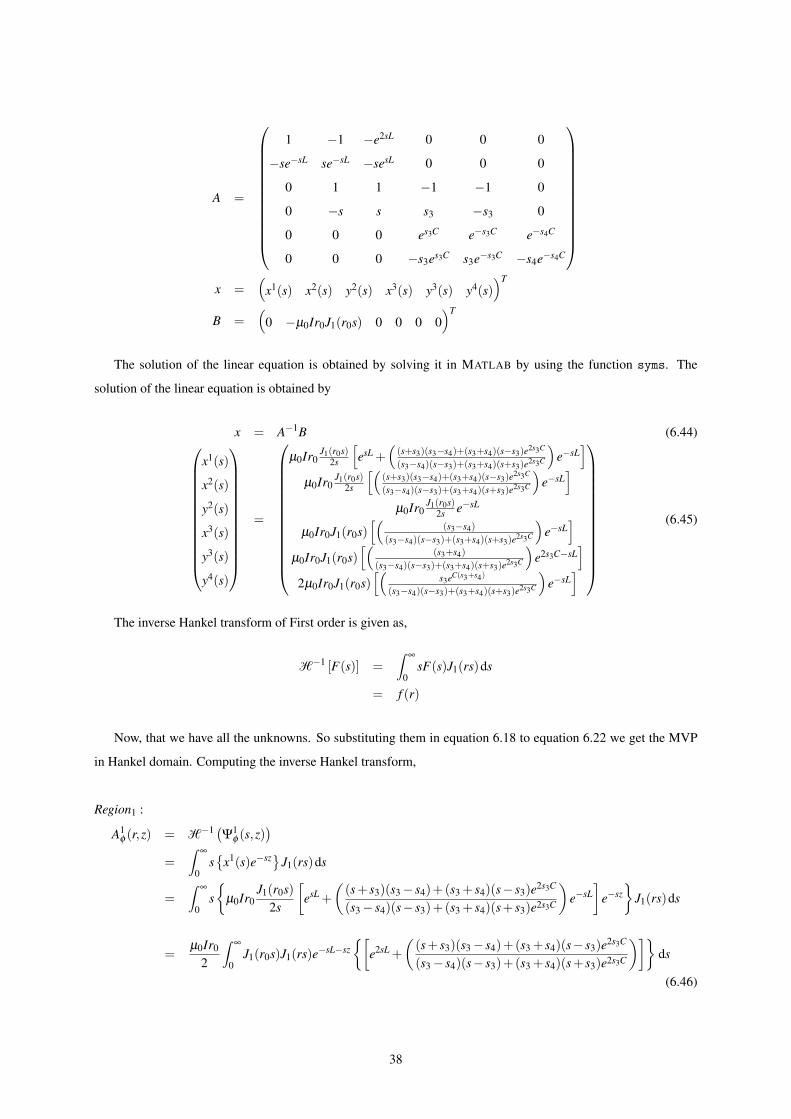
The solution of the linear equation is obtained by solving it in MATLAB by using the function syms. The
solution of the linear equation is obtained by
x = A−1B (6.44)
x1(s)
x2(s)
y2(s)
x3(s)
y3(s)
y4(s)
=
µ0Ir0J1(r0s)
2s
[esL +
((s+s3)(s3−s4)+(s3+s4)(s−s3)e2s3C
(s3−s4)(s−s3)+(s3+s4)(s+s3)e2s3C
)e−sL
]µ0Ir0
J1(r0s)2s
[((s+s3)(s3−s4)+(s3+s4)(s−s3)e2s3C
(s3−s4)(s−s3)+(s3+s4)(s+s3)e2s3C
)e−sL
]µ0Ir0
J1(r0s)2s e−sL
µ0Ir0J1(r0s)[(
(s3−s4)
(s3−s4)(s−s3)+(s3+s4)(s+s3)e2s3C
)e−sL
]µ0Ir0J1(r0s)
[((s3+s4)
(s3−s4)(s−s3)+(s3+s4)(s+s3)e2s3C
)e2s3C−sL
]2µ0Ir0J1(r0s)
[(s3eC(s3+s4)
(s3−s4)(s−s3)+(s3+s4)(s+s3)e2s3C
)e−sL
]
(6.45)
The inverse Hankel transform of First order is given as,
H−1 [F(s)] =∫
∞
0sF(s)J1(rs)ds
= f (r)
Now, that we have all the unknowns. So substituting them in equation 6.18 to equation 6.22 we get the MVP
in Hankel domain. Computing the inverse Hankel transform,
Region1 :
A1φ (r,z) = H−1 (
Ψ1φ (s,z)
)=
∫∞
0s{
x1(s)e−sz}J1(rs)ds
=∫
∞
0s{
µ0Ir0J1(r0s)
2s
[esL +
((s+ s3)(s3− s4)+(s3 + s4)(s− s3)e2s3C
(s3− s4)(s− s3)+(s3 + s4)(s+ s3)e2s3C
)e−sL
]e−sz
}J1(rs)ds
=µ0Ir0
2
∫∞
0J1(r0s)J1(rs)e−sL−sz
{[e2sL +
((s+ s3)(s3− s4)+(s3 + s4)(s− s3)e2s3C
(s3− s4)(s− s3)+(s3 + s4)(s+ s3)e2s3C
)]}ds
(6.46)
38
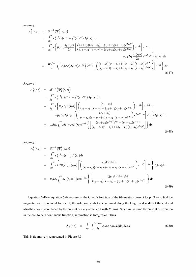
Region2 :
A2φ (r,z) = H−1 (
Ψ2φ (s,z)
)=
∫∞
0s{
x2(s)e−sz + y2(s)esz}J1(rs)ds
=∫
∞
0s{
µ0Ir0J1(r0s)
2s
[((s+ s3)(s3− s4)+(s3 + s4)(s− s3)e2s3C
(s3− s4)(s− s3)+(s3 + s4)(s+ s3)e2s3C
)e−sL
]e−sz . . .
. +µ0Ir0J1(r0s)
2se−sLesz
}J1(rs)ds
=µ0Ir0
2
∫∞
0J1(r0s)J1(rs)e−sL
{esz +
[((s+ s3)(s3− s4)+(s3 + s4)(s− s3)e2s3C
(s3− s4)(s− s3)+(s3 + s4)(s+ s3)e2s3C
)]e−sz
}ds
(6.47)
Region3 :
A3φ (r,z) = H−1
(Ψ
3φ (s,z)
)=
∫∞
0s{
x3(s)e−s3z + y3(s)es3z}J1(rs)ds
=∫
∞
0s{
µ0Ir0J1(r0s)[(
(s3− s4)
(s3− s4)(s− s3)+(s3 + s4)(s+ s3)e2s3C
)e−sL
]e−s3z . . .
. +µ0Ir0J1(r0s)[(
(s3 + s4)
(s3− s4)(s− s3)+(s3 + s4)(s+ s3)e2s3C
)e2s3C−sL
]es3z}
J1(rs)ds
= µ0Ir0
∫∞
0sJ1(r0s)J1(rs)e−sL
{[(s3 + s4)e2s3Ces3z +(s3− s4)e−s3z
(s3− s4)(s− s3)+(s3 + s4)(s+ s3)e2s3C
]}ds
(6.48)
Region4 :
A4φ (r,z) = H−1 (
Ψ4φ (s,z)
)=
∫∞
0s{
y4(s)es4z}J1(rs)ds
=∫
∞
0s
{2µ0Ir0J1(r0s)
[(s3eC(s3+s4)
(s3− s4)(s− s3)+(s3 + s4)(s+ s3)e2s3C
)e−sL
]es4z
}J1(rs)ds
= µ0Ir0
∫∞
0sJ1(r0s)J1(rs)e−sL
{[2s3eC(s3+s4)es4z
(s3− s4)(s− s3)+(s3 + s4)(s+ s3)e2s3C
]}ds
(6.49)
Equation 6.46 to equation 6.49 represents the Green’s function of the filamentary current loop. Now to find the
magnetic vector potential for a coil, the solution needs to be summed along the length and width of the coil and
also the current is replaced by the current density of the coil with N turns. Since we assume the current distribution
in the coil to be a continuous function, summation is Integration. Thus
Aφ (r,z) =∫
∞
0
∫ r2
r1
∫ L2
L1
Aφ (r,z,r0,L)dr0dLds (6.50)
This is figuratively represented in Figure 6.3
39
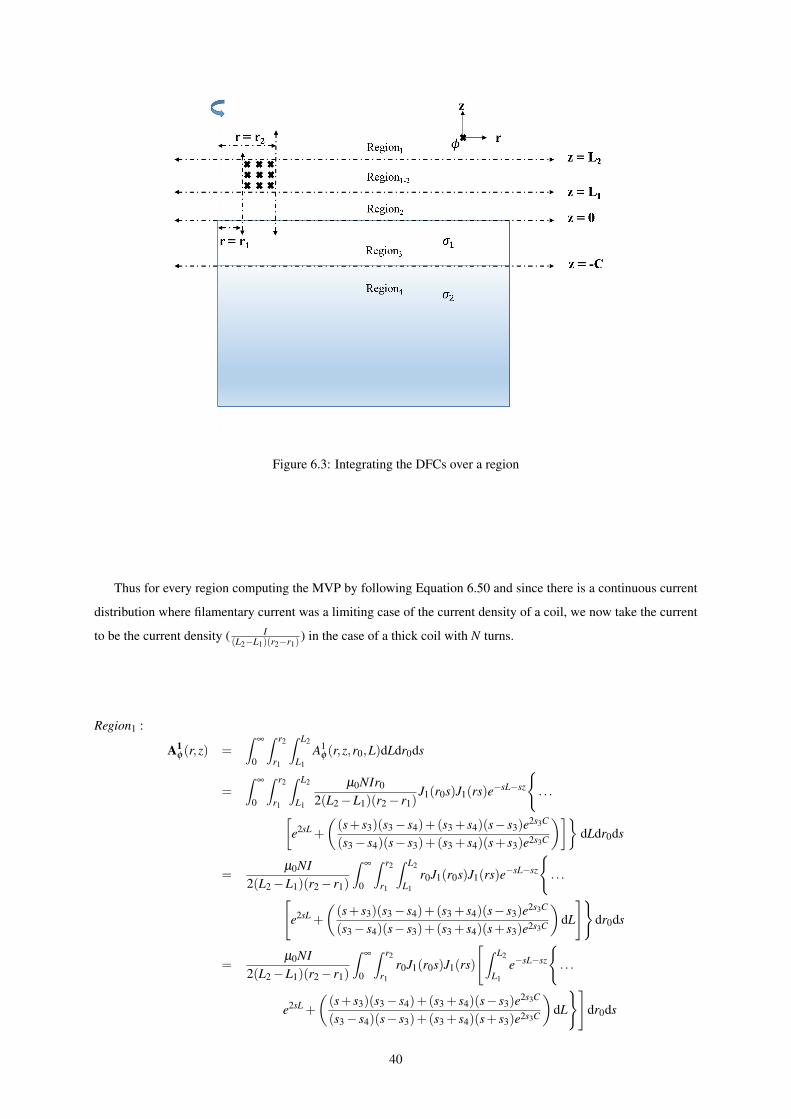
Figure 6.3: Integrating the DFCs over a region
Thus for every region computing the MVP by following Equation 6.50 and since there is a continuous current
distribution where filamentary current was a limiting case of the current density of a coil, we now take the current
to be the current density ( I(L2−L1)(r2−r1)
) in the case of a thick coil with N turns.
Region1 :
A1φ (r,z) =
∫∞
0
∫ r2
r1
∫ L2
L1
A1φ (r,z,r0,L)dLdr0ds
=∫
∞
0
∫ r2
r1
∫ L2
L1
µ0NIr0
2(L2−L1)(r2− r1)J1(r0s)J1(rs)e−sL−sz
{. . .
.
[e2sL +
((s+ s3)(s3− s4)+(s3 + s4)(s− s3)e2s3C
(s3− s4)(s− s3)+(s3 + s4)(s+ s3)e2s3C
)]}dLdr0ds
=µ0NI
2(L2−L1)(r2− r1)
∫∞
0
∫ r2
r1
∫ L2
L1
r0J1(r0s)J1(rs)e−sL−sz
{. . .
.
[e2sL +
((s+ s3)(s3− s4)+(s3 + s4)(s− s3)e2s3C
(s3− s4)(s− s3)+(s3 + s4)(s+ s3)e2s3C
)dL
]}dr0ds
=µ0NI
2(L2−L1)(r2− r1)
∫∞
0
∫ r2
r1
r0J1(r0s)J1(rs)
[∫ L2
L1
e−sL−sz
{. . .
. e2sL +
((s+ s3)(s3− s4)+(s3 + s4)(s− s3)e2s3C
(s3− s4)(s− s3)+(s3 + s4)(s+ s3)e2s3C
)dL
}]dr0ds
40
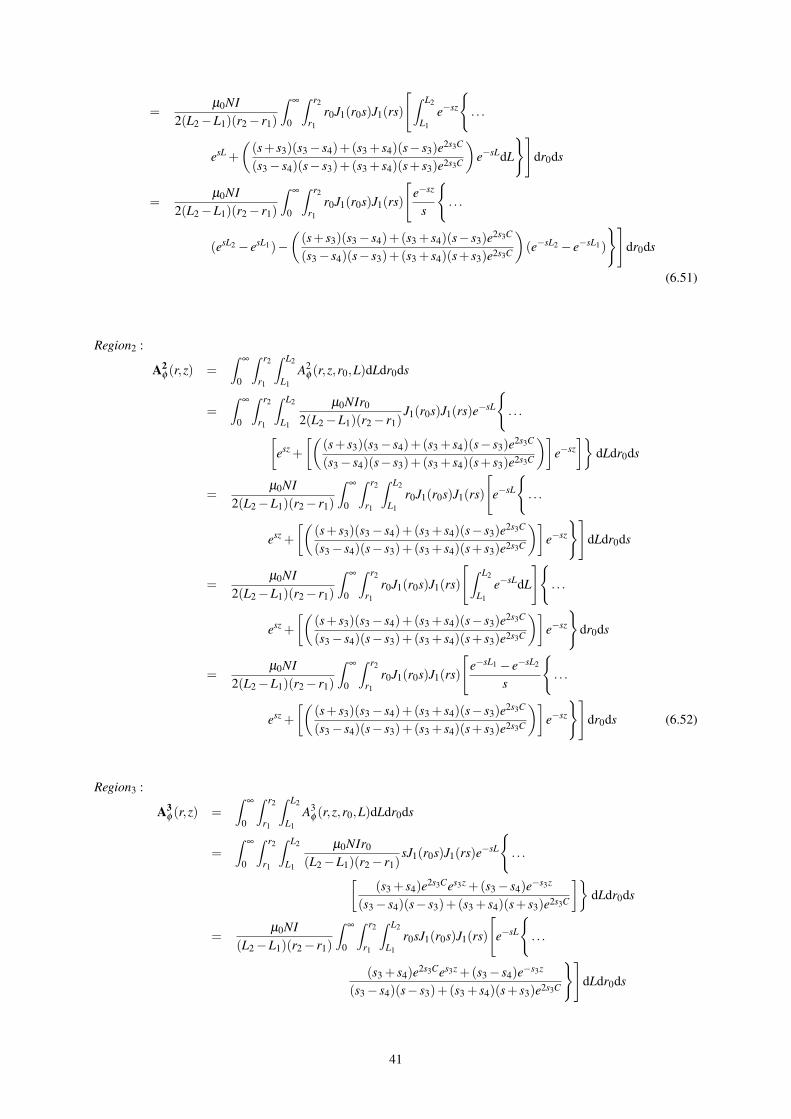
=µ0NI
2(L2−L1)(r2− r1)
∫∞
0
∫ r2
r1
r0J1(r0s)J1(rs)
[∫ L2
L1
e−sz
{. . .
. esL +
((s+ s3)(s3− s4)+(s3 + s4)(s− s3)e2s3C
(s3− s4)(s− s3)+(s3 + s4)(s+ s3)e2s3C
)e−sLdL
}]dr0ds
=µ0NI
2(L2−L1)(r2− r1)
∫∞
0
∫ r2
r1
r0J1(r0s)J1(rs)
[e−sz
s
{. . .
. (esL2 − esL1)−((s+ s3)(s3− s4)+(s3 + s4)(s− s3)e2s3C
(s3− s4)(s− s3)+(s3 + s4)(s+ s3)e2s3C
)(e−sL2 − e−sL1)
}]dr0ds
(6.51)
Region2 :
A2φ (r,z) =
∫∞
0
∫ r2
r1
∫ L2
L1
A2φ (r,z,r0,L)dLdr0ds
=∫
∞
0
∫ r2
r1
∫ L2
L1
µ0NIr0
2(L2−L1)(r2− r1)J1(r0s)J1(rs)e−sL
{. . .
.
[esz +
[((s+ s3)(s3− s4)+(s3 + s4)(s− s3)e2s3C
(s3− s4)(s− s3)+(s3 + s4)(s+ s3)e2s3C
)]e−sz
]}dLdr0ds
=µ0NI
2(L2−L1)(r2− r1)
∫∞
0
∫ r2
r1
∫ L2
L1
r0J1(r0s)J1(rs)
[e−sL
{. . .
. esz +
[((s+ s3)(s3− s4)+(s3 + s4)(s− s3)e2s3C
(s3− s4)(s− s3)+(s3 + s4)(s+ s3)e2s3C
)]e−sz
}]dLdr0ds
=µ0NI
2(L2−L1)(r2− r1)
∫∞
0
∫ r2
r1
r0J1(r0s)J1(rs)
[∫ L2
L1
e−sLdL
]{. . .
. esz +
[((s+ s3)(s3− s4)+(s3 + s4)(s− s3)e2s3C
(s3− s4)(s− s3)+(s3 + s4)(s+ s3)e2s3C
)]e−sz
}dr0ds
=µ0NI
2(L2−L1)(r2− r1)
∫∞
0
∫ r2
r1
r0J1(r0s)J1(rs)
[e−sL1 − e−sL2
s
{. . .
. esz +
[((s+ s3)(s3− s4)+(s3 + s4)(s− s3)e2s3C
(s3− s4)(s− s3)+(s3 + s4)(s+ s3)e2s3C
)]e−sz
}]dr0ds (6.52)
Region3 :
A3φ (r,z) =
∫∞
0
∫ r2
r1
∫ L2
L1
A3φ (r,z,r0,L)dLdr0ds
=∫
∞
0
∫ r2
r1
∫ L2
L1
µ0NIr0
(L2−L1)(r2− r1)sJ1(r0s)J1(rs)e−sL
{. . .
.
[(s3 + s4)e2s3Ces3z +(s3− s4)e−s3z
(s3− s4)(s− s3)+(s3 + s4)(s+ s3)e2s3C
]}dLdr0ds
=µ0NI
(L2−L1)(r2− r1)
∫∞
0
∫ r2
r1
∫ L2
L1
r0sJ1(r0s)J1(rs)
[e−sL
{. . .
.(s3 + s4)e2s3Ces3z +(s3− s4)e−s3z
(s3− s4)(s− s3)+(s3 + s4)(s+ s3)e2s3C
}]dLdr0ds
41

=µ0NI
(L2−L1)(r2− r1)
∫∞
0
∫ r2
r1
r0sJ1(r0s)J1(rs)
[∫ L2
L1
e−sLdL
]{. . .
.(s3 + s4)e2s3Ces3z +(s3− s4)e−s3z
(s3− s4)(s− s3)+(s3 + s4)(s+ s3)e2s3C
}dr0ds
=µ0NI
(L2−L1)(r2− r1)
∫∞
0
∫ r2
r1
r0J1(r0s)J1(rs)
[(e−sL1 − e−sL2)
{. . .
.(s3 + s4)e2s3Ces3z +(s3− s4)e−s3z
(s3− s4)(s− s3)+(s3 + s4)(s+ s3)e2s3C
}]dr0ds (6.53)
Region4 :
A4φ (r,z) =
∫∞
0
∫ r2
r1
∫ L2
L1
A4φ (r,z,r0,L)dLdr0ds
=∫
∞
0
∫ r2
r1
∫ L2
L1
µ0NIr0
(L2−L1)(r2− r1)sJ1(r0s)J1(rs)e−sL
{. . .
.
[2s3eC(s3+s4)es4z
(s3− s4)(s− s3)+(s3 + s4)(s+ s3)e2s3C
]}dLdr0ds
=µ0NI
(L2−L1)(r2− r1)
∫∞
0
∫ r2
r1
∫ L2
L1
r0sJ1(r0s)J1(rs)
[e−sL
{. . .
.2s3eC(s3+s4)es4z
(s3− s4)(s− s3)+(s3 + s4)(s+ s3)e2s3C
}]dLdr0ds
=µ0NI
(L2−L1)(r2− r1)
∫∞
0
∫ r2
r1
r0sJ1(r0s)J1(rs)
[∫ L2
L1
e−sLdL
]{. . .
.2s3eC(s3+s4)es4z
(s3− s4)(s− s3)+(s3 + s4)(s+ s3)e2s3C
}dr0ds
=µ0NI
(L2−L1)(r2− r1)
∫∞
0
∫ r2
r1
r0J1(r0s)J1(rs)
[(e−sL1 − e−sL2)
{. . .
.2s3eC(s3+s4)es4z
(s3− s4)(s− s3)+(s3 + s4)(s+ s3)e2s3C
}]dr0ds (6.54)
Equations 6.51 to 6.54 represents the vector potential generated by a coil of cross section area (L2−L1)(r2−r1)
from Region1 to Region4. But the region in which the coil is present has not been identified yet. In this region,
there is an intersection of Region1 and Region2 at any point in this region. So the random point is assigned the
co-ordinate (r,ζ )=(r0,z). It is to be noted that the co-ordinate of z has been changed to ζ . It is not going to affect
the results in anyway, because it is a dummy variable in the integral equation. This is used to distinguish between
the co-ordinate and a random point in the co-ordinate. So, in the sub-region between (r,ζ = z) to (r,ζ = L2),
A1φ(r,ζ ) is valid (Equation 6.46) and in the sub-region between (r,ζ = L1) to (r,ζ = z), A2
φ(r,ζ ) is valid (Equation
6.47). This is graphically represented in Figure 6.4
To obtain obtain the vector potential in the region of the coil, first the DFC has to be summed (integrated
42

Figure 6.4: Pictorial representation of the problem in new co-ordinates and selecting the sub-regions for computingA1−2
φ(r,z)
in continuous case) along the ζ axis obeying the conditions mentioned in the previous paragraph. Then this
solution has to be summed (integrated in continuous case) along the radius in which the coil is defined. This
is perfectly valid because the governing differential equation is linear and thus the possibility to compute the
integration individually. This is shown diagrammatically in Figure 6.5
Figure 6.5: Summing the solution of a DFC, first along ζ and then along r
Region1−2 :
A1−2φ
(r,z) =∫ r2
r1
⟨∫ z
L1
A2φ dζ +
∫ L2
zA1
φ dζ
⟩dr0
=∫ r2
r1
⟨∫ z
L1
µ0i0r0
2
∫∞
0J1(r0s)J1(rs)e−sz
{esζ +
[((s+ s3)(s3− s4)+(s3 + s4)(s− s3)e2s3C
(s3− s4)(s− s3)+(s3 + s4)(s+ s3)e2s3C
)]. . .
. e−sζ
}dsdζ +
∫ L2
z
µ0NIr0
2(L2−L1)(r2− r1)
∫∞
0J1(r0s)J1(rs)e−sz−sζ
{[e2sz + . . .
.
((s+ s3)(s3− s4)+(s3 + s4)(s− s3)e2s3C
(s3− s4)(s− s3)+(s3 + s4)(s+ s3)e2s3C
)]}dsdζ
⟩dr0
43
=µ0i0
2
∫∞
0
∫ r2
r1
r0J1(r0s)J1(rs)
⟨∫ z
L1
e−sz{
esζ +
[((s+ s3)(s3− s4)+(s3 + s4)(s− s3)e2s3C
(s3− s4)(s− s3)+(s3 + s4)(s+ s3)e2s3C
)]. . .
. e−sζ
}dζ +
∫ L2
ze−sz−sζ
{[e2sz +
((s+ s3)(s3− s4)+(s3 + s4)(s− s3)e2s3C
(s3− s4)(s− s3)+(s3 + s4)(s+ s3)e2s3C
)]}dζ
⟩dr0ds
=µ0NI
2(L2−L1)(r2− r1)
∫∞
0
∫ r2
r1
r0J1(r0s)J1(rs)s
{2− e−s(z−L1)− es(z−L2)+ . . .
.
[e−sz
((s+ s3)(s3− s4)+(s3 + s4)(s− s3)e2s3C
(s3− s4)(s− s3)+(s3 + s4)(s+ s3)e2s3C
)(e−sL1 − e−sL1
)]}dr0ds
(6.55)
Thus we have the MVP generated by a coil of finite thickness in the vicinity of 2 stacked conducting plates
which is given as per Equation 6.51 to Equation 6.55.
6.4 Invariance of Magnetic Field
In the previous section, we derived the field equations of the vector potential in various regions of a coil over two
plates. With the vector potential it is possible to obtain the magnetic field [3] by just considering the equation
6.22. In order to prove and validate the principle it is sufficient to consider just one of the regions and validate the
dilation invariance.
Let us consider the MVP in Region3 (A3φ(r,z)) from equation 6.53. Evaluating the Br and Bz components by
using equation 6.22 and referring io = NI(L2−L1)(r2−r1)
, we get
B3r = −
∂A3φ
∂ z
= − ∂
∂ z
[µ0i0
∫∞
0
∫ r2
r1
r0J1(r0s)J1(rs)
[(e−sL1 − e−sL2)
{. . .
.(s3 + s4)e2s3Ces3z +(s3− s4)e−s3z
(s3− s4)(s− s3)+(s3 + s4)(s+ s3)e2s3C
}]dr0ds
]
= − ∂
∂ z
[µ0i0
∫∞
0
(∫ r2
r1
r0J1(r0s)dr0
)J1(rs)
[(e−sL1 − e−sL2)
{. . .
.(s3 + s4)e2s3Ces3z +(s3− s4)e−s3z
(s3− s4)(s− s3)+(s3 + s4)(s+ s3)e2s3C
}]ds
]
= µ0i0∫
∞
0s3
(∫ r2
r1
r0J1(r0s)dr0
)J1(rs)
[(e−sL1 − e−sL2)
{. . .
.(s3− s4)e−s3z− (s3 + s4)e2s3Ces3z
(s3− s4)(s− s3)+(s3 + s4)(s+ s3)e2s3C
}]ds (6.56)
44
B3z =
1r
∂ rA3φ
∂ r
=1r
∂
∂ r
[rµ0i0
∫∞
0
∫ r2
r1
r0J1(r0s)J1(rs)
[(e−sL1 − e−sL2)
{. . .
.(s3 + s4)e2s3Ces3z +(s3− s4)e−s3z
(s3− s4)(s− s3)+(s3 + s4)(s+ s3)e2s3C
}]dr0ds
]
=1r
∂
∂ r
[rµ0i0
∫∞
0
(∫ r2
r1
r0J1(r0s)dr0
)J1(rs)
[(e−sL1 − e−sL2)
{. . .
.(s3 + s4)e2s3Ces3z +(s3− s4)e−s3z
(s3− s4)(s− s3)+(s3 + s4)(s+ s3)e2s3C
}]ds
]
=1r
µ0i0∫
∞
0
(∫ r2
r1
r0J1(r0s)dr0
)(∂
∂ rrJ1(rs)
)[(e−sL1 − e−sL2)
{. . .
.(s3 + s4)e2s3Ces3z +(s3− s4)e−s3z
(s3− s4)(s− s3)+(s3 + s4)(s+ s3)e2s3C
}]ds
=1r
µ0i0∫
∞
0
(∫ r2
r1
r0J1(r0s)dr0
)(1s
∂
∂ rrsJ1(rs)
)[(e−sL1 − e−sL2)
{. . .
.(s3 + s4)e2s3Ces3z +(s3− s4)e−s3z
(s3− s4)(s− s3)+(s3 + s4)(s+ s3)e2s3C
}]ds (6.57)
Consider only 1s
∂
∂ r rsJ1(rs) from equation 6.57 which needs to be simplified.
Substitute rs = x ⇒ s∂ r = ∂x. So,
1s
∂
∂ rrsJ1(rs) =
∂
∂xxJ1(x)
∂
∂xxJ1(x) = xJ0(x)
xJ0(x) = rsJ0(rs) (6.58)
Substituting equation 6.58 in equation 6.57, we get
Bz =1r
µ0i0∫
∞
0
(∫ r2
r1
r0J1(r0s)dr0
)(rsJ0(rs)
)[(e−sL1 − e−sL2)
{. . .
.(s3 + s4)e2s3Ces3z +(s3− s4)e−s3z
(s3− s4)(s− s3)+(s3 + s4)(s+ s3)e2s3C
}]ds (6.59)
Analytical closed form expression for equation 6.56 and equation 6.59 doesn’t exist. However they can be
numerically computed to visualize the nature of Br and Bz inside the plate [3]. There are several methods to
compute the double integrals numerically. One of them is Monte Carlo method [1, 9], which has been used to
evaluate the double integrals. The other quadrature techniques (Riemann summation, Trapezoidal rule etc.) are
computationally intensive and take a long time to compute.
In the method of Monte Carlo, there has to be a set of random numbers generated in the region under which the
integral is being computed [22]. But one of the variables has an upper limit of ∞. So to overcome this difficulty,
the upper limit was taken to be a large number. The reason for restricting the upper limit is that the magnetic flux
45

density and the vector potential are square integrable functions, meaning that they are finite values in space. So the
function tends to reduce and become insignificant for higher values of s. It is mathematically represented below,
by considering the case for magnetic vector potential. This also applies to the case of magnetic flux density which
was derived from the magnetic vector potential.
A3φ (r,z) = µ0i0
∫∞
0
∫ r2
r1
r0J1(r0s)J1(rs)
[(e−sL1 − e−sL2)
{(s3 + s4)e2s3Ces3z +(s3− s4)e−s3z
(s3− s4)(s− s3)+(s3 + s4)(s+ s3)e2s3C
}]dr0ds
≈ limλ→∞
µ0i0∫
λ
0
∫ r2
r1
r0J1(r0s)J1(rs)
[(e−sL1 − e−sL2)
{. . .
.(s3 + s4)e2s3Ces3z +(s3− s4)e−s3z
(s3− s4)(s− s3)+(s3 + s4)(s+ s3)e2s3C
}]dr0ds
Generating random numbers in the required region need not be uniformly distributed i.e. their concentration
may vary. So a version of stratified sampling for Monte Carlo method was used, in order to make sure the distri-
bution of points is uniform. In order to demonstrate this, a histogram plot of the random sampling has been made.
The histogram plot gives the relative frequency of the occurrence of points in the bins. It is represented only for
the case of r0 and is depicted in the below figure.
0.012 0.01210.01210.01220.01220.01230.01230.01240.01240.01259200
9400
9600
9800
10000
10200
10400
10600
r0
Rel
ativ
e F
requ
ency
(a) Non-Uniform distribution of points
0.012 0.0121 0.0122 0.0123 0.0124 0.0125
9400
9600
9800
10000
10200
10400
10600
r0
Rel
ativ
e F
requ
ency
(b) Uniform distribution of points
Figure 6.6: Histogram plot of distribution of points in each stratum
From figure 6.6 (a) it is clear that the points are not uniformly distributed. It is because of the random sampling,
without any prior distribution. From figure 6.6 (b) it can be seen that the points are uniformly distributed in the
bins. This can be achieved by using the method sampling by stratification, wherein, the region under consideration
is stratified and each stratified region is sampled individually. In this case stratification was achieved by generating
random integers for the required total number of samples and then these integers were scaled between the regions.
The MATLAB command that generates random integers is randperm(Nsamples). The plot of the equation 6.56 and
equation 6.57 for the case of a single conductive plate (by taking s4 = s) are depicted in figure 6.7 for the situation
of k = 1.
46
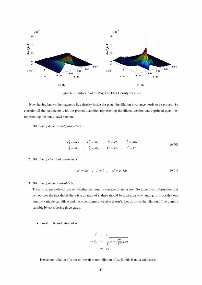
00.01
0.020.03
0.04
0
1
2
x 10−3
0
2
4
6
x 10−3
r / m−z / m
abs(
B r) / T
(a) Br
00.01
0.020.03
0.04
0
1
2
x 10−3
0
2
4
6
x 10−4
r / m−z / m
abs(
B z) / T
(b) Bz
Figure 6.7: Surface plot of Magnetic Flux Density for k = 1
Now, having known the magnetic flux density inside the plate, the dilation invariance needs to be proved. So
consider all the parameters with the primed quantities representing the dilated version and unprimed quantities
representing the non-dilated version.
1. Dilation of dimensional parameters :
L′1 = kL1 , L′2 = kL2 , z′ = kz , r′0 = kr0
r′1 = kr1 , r′2 = kr2 , C′ = kC , r′ = kr(6.60)
2. Dilation of electrical parameters :
N′ = kN , I′ = I , ω ′ = k−2ω (6.61)
3. Dilation of dummy variable (s) :
There is no pre-defined rule on whether the dummy variable dilate or not. So to get this information, Let
us consider the fact that if there is a dilation of s, there should be a dilation of s3 and s4. It is not that one
dummy variable can dilate and the other dummy variable doesn’t. Let us prove the dilation of the dummy
variable by considering three cases.
• case-1 : Non-dilation of s-
s′ = s
⇒ s′3 =
√s2 + j
ω
k2 µ0σ3
6= s3
Hence non-dilation of s doesn’t result in non-dilation of s3. So this is not a valid case.
47

• case-2 : Dilation of s by k times-
s′ = ks
⇒ s′3 =
√(ks)2 + j
ω
k2 µ0σ3
6= ks3
Hence dilation of s by k times doesn’t result in dilation of s3 by k times. So this is not a valid case.
• case-3 : Dilation of s by 1k times-
s′ =sk
⇒ s′3 =
√(sk
)2
+ jω
k2 µ0σ3
⇒ s′3 =
√1k2
(s2 + jωµ0σ3
)=
s3
k
Hence dilation of s by 1k times results in dilation of s3 by 1
k times. So this is a valid case.
Hence with this small case study we have proved the dilation of the dummy variable.
s′ = sk , s′3 =
s3k , s′4 =
s4k
(6.62)
Now consider the dilated version of Br and Bz (represented as B′r and B′z) from equation 6.56 and equation
6.59 we have,
B′r = µ0i′0
∫∞
0s′3
(∫ r′2
r′1r′0J1(r′0s′)dr′0
)J1(r′s′)
[(e−s′L′1 − e−sL′2)
{. . .
.(s′3− s′4)e
−s′3z′ − (s′3 + s′4)e2s′3C′es′3z′
(s′3− s′4)(s′− s′3)+(s′3 + s′4)(s
′+ s′3)e2s′3C′
}]ds′ (6.63)
B′z =1r′
µ0i′0
∫∞
0
(∫ r′2
r′1r′0J1(r′0s′)dr′0
)(r′s′J0(r′s′)
)[(e−s′L′1 − e−s′L′2)
{. . .
.(s′3 + s′4)e
2s′3C′es′3z′ +(s′3− s′4)e−s′3z′
(s′3− s′4)(s′− s′3)+(s′3 + s′4)(s
′+ s′3)e2s′3C′
}]ds′ (6.64)
Now the task is to substitute the dilation parameters considered in the set of equations of 6.60, 6.61, 6.62 and
substitute it in B′r and B′z of equation 6.63 and 6.64, we obtain (Refer Appendix B for the proof)
B′r = µ0i0∫
∞
0s3
(∫ r2
r1
r0J1(r0s)dr0
)J1(rs)
[(e−sL1 − e−sL2)
{(s3− s4)e−s3z− (s3 + s4)e2s3Ces3z
(s3− s4)(s− s3)+(s3 + s4)(s+ s3)e2s3C
}]ds
= Br
B′z =1r
µ0i0∫
∞
0
(∫ r2
r1
r0J1(r0s)dr0
)(rsJ0(rs)
)[(e−sL1 − e−sL2)
{(s3 + s4)e2s3Ces3z +(s3− s4)e−s3z
(s3− s4)(s− s3)+(s3 + s4)(s+ s3)e2s3C
}]ds
= Bz
48
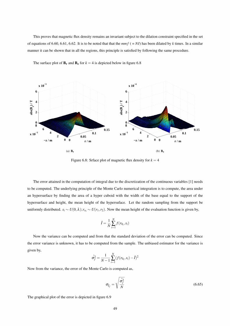
This proves that magnetic flux density remains an invariant subject to the dilation constraint specified in the set
of equations of 6.60, 6.61, 6.62. It is to be noted that that the mm f ( = NI) has been dilated by k times. In a similar
manner it can be shown that in all the regions, this principle is satisfied by following the same procedure.
The surface plot of Br and Bz for k = 4 is depicted below in figure 6.8
00.05
0.10.15
02
46
8
x 10−3
0
2
4
6
x 10−3
r / m−z / m
abs(
B r) / T
(a) Br
00.05
0.10.15
02
46
8
x 10−3
0
2
4
6
x 10−4
r / m−z / m
abs(
B z) / T
(b) Bz
Figure 6.8: Srface plot of magnetic flux density for k = 4
The error attained in the computation of integral due to the discretization of the continuous variables [1] needs
to be computed. The underlying principle of the Monte Carlo numerical integration is to compute, the area under
an hypersurface by finding the area of a hyper cuboid with the width of the base equal to the support of the
hypersurface and height, the mean height of the hypersuface. Let the random sampling from the support be
uniformly distributed. si ∼ U(0,λ );roi ∼ U(r1,r2). Now the mean height of the evaluation function is given by,
I =1N
N
∑i=1
f (r0i ,si)
Now the variance can be computed and from that the standard deviation of the error can be computed. Since
the error variance is unknown, it has to be computed from the sample. The unbiased estimator for the variance is
given by,
σ2f =
1N−1
N
∑i=1
( f (r0i ,si)− I)2
Now from the variance, the error of the Monte Carlo is computed as,
σI f=
√σ2
f
N(6.65)
The graphical plot of the error is depicted in figure 6.9
49

0
0.02
0.04
0
1
2
x 10−3
0
2
4
6
8
x 10−7
r−z
|err
or|
(a) Br
0
0.02
0.04
0
1
2
x 10−3
0
1
2
3
4
x 10−7
r−z
|err
or|
(b) Bz
Figure 6.9: Numerical Integration error for k = 1
It is clear from the magnitude plot that the maximum error is less than 4×10⁻⁷, which is much less than the
magnitude of the magnetic flux density. The ratio of the plots of the magnetic flux density for both the components
of the two cases is also computed and plotted in figure 6.10
00.01
0.020.03
0.04
00.5
11.5
2
x 10−3
0.99
0.995
1
1.005
1.01
1.015
r / m−z / m
|Rat
io|
(a) Ratio of Br for k = 1 and k = 4
00.01
0.020.03
0.04
00.5
11.5
2
x 10−3
0.98
0.99
1
1.01
1.02
1.03
r / m−z / m
|Rat
io|
(b) Ratio of Bz for k = 1 and k = 4
Figure 6.10: Ratio of the absolute values of the individual components of the magnetic flux density
It can be seen from the figure 6.10 that the ratio is not exactly 1. The reason can be attributed to the error due
to discretisation involved in computing the integral numerically. But overall the results lie in a agreeable variance
from the desired value of 1.
50
Chapter 7
Conclusions
This thesis mainly focus on the proof of concept of the dilation invariance principle. According to this principle
dilation of the dimensional and electrical parameters of the probe, plate and the crack, should make the magnetic
field an invariant, provided the measurement are carried out at the dilated points. Accordingly, several experiments
and finite element based simulations were conducted in order to prove the principle. Finally the principle was
proved analytically by considering a reduced version of the original model.
7.1 Experimental Study
In the experimental study, notches were machined on Al1050 plates, that are dimensionally dilated. Two probes
were built that were also dimensionally dilated and excited by current and frequencies that obey the dilation param-
eters. The x-y positioning system, positions the probe at the desired (dilated) location on the notch.The parameters
of the detected signal were estimated by a 3 parameter sine fitting algorithm. The obtained signal amplitude for
the horizontal and vertical scans for both the case studies were compared.
There were some ambiguities in the results which is due to the non-positioning of the sensor and the probe
on the exactly dilated point. Also the ambiguities arise due to the inexact winding of the coil. The experiments
utilized GMR (NVE-AA002) sensor to measure the magnetic field, which can sense the field only along one axis,
in this case the x-axis. Since the GMR sensor is fixed (immobile) to the probe, measurement of other components
of the magnetic field becomes infeasible. So this forces us to adopt simulation study.
7.2 Simulation Study
The problem under study was simulated in a finite element based simulation software. All the dimensional pa-
rameters of the notch, plate thickness and the probe; electrical parameters of the probe were same as that of the
experimental study. The plate had the same properties of Al1050. The only difference was that the probe was kept
at a constant position and the crack moved relative to the center of the probe. A plot of the x-component of the
magnetic field and the z-component of the magnetic field were made for the horizontal scan and the vertical scan
51
for both the case studies. There was a good match in the results.
In the case of simulations some minor ambiguities were noted. These ambiguities were mainly due to the
meshing of the domain under study. All the region need to be finely meshed in order to get a perfect solution. But
a fine mesh would create a huge amount of independent variables that need to be solved. The desktop PC may not
be able to solve it or take it a long time to solve. So in order to avoid it, fine mesh is created only at the desired
region and then made coarser progressively. This resulted in a fairly better result and took a lesser duration of time
to solve. There are however many other parameters that need to be considered in order to obtain better results.
7.3 Analytical Study
The analytical study involved in formulating the desired field equation, considering the current sheet approxima-
tion for the coil, for a filamentary current loop. This gives the Green’s function of the variable under consideration
in the field equation, which is the magnetic vector potential. A simplification of the geometry has been assumed,
which is that the geometry of the plate under consideration is a cylinder of infinite radius and finite thickness. Since
the geometry has a cylindrical symmetry, it would be easier to consider the vector Laplacian in the field equation in
cylindrical coordinates (only the azimuthal component). Any derivatives with respect to the azimuthal component
is taken to be 0, because of the symmetry.
First order Hankel transform is computed and the resulting differential equation, which would be a second order
linear differential equation with constant coefficients, is solved to get the Green’s function. The constants of the
solution are found from the boundary condition in the transformed domain. It is done by analysing the continuity
of the electric field and magnetic flux density at the surface of the boundary. The full solution is obtained by
integrating the Green’s function in the region defined by the cross section of the coil. From the magnetic vector
potential, the magnetic flux density is computed. It is plotted in MATLAB and hence the dilation invariance of the
magnetic flux density is proved by comparing the plot of both cases. The integration was carried out numerically
using the stratified Monte Carlo technique.
52

Bibliography
[1] Monte carlo integration. http://ta.twi.tudelft.nl/mf/users/oosterle/oosterlee/
lec8-hit-2009.pdf. Accessed: 2016-09-10.
[2] Venkatraman B., Raj B., and Rao B.P.C. Pratical Eddy Current Testing. Alpha Science, 2007.
[3] Prashanth Baskaran, A. Lopes Ribeiro, and H. Geirinhas Ramos. The dilation invariance principle in eddy-
current non-destructive evaluation technique - analytical justification. Accepted, May 2017.
[4] Jack Blitz. Electrical and Magnetic Methods of Non-destructive Testing. Springer Science, 2nd edition.
[5] C.V. Dodd and W.E. Deed. Analytical solution to eddy current probe-coil problems. Journal of Applied
Physics, 1968.
[6] T. Dogaru and S.T. Smith. Giant magnetoresistance-based eddy-current sensor. IEEE Transactions on Mag-
netics, 2001.
[7] Lawrence Evans. Partial Differential Equations. American Mathematical Society, 1998.
[8] Bradley Harding, Christophe Tremblay, and Denis Cousineau. Standard errors: A review and evaluation of
standard error estimators using monte carlo simulations. The Quantitative Methods for Psychology, 2014.
[9] Wojciech Jarosz. Efficient Monte Carlo Methods for Light Transport in Scattering Media. PhD thesis, UC
San Diego, September 2008.
[10] R. Ko and M. Blodgett. Application of a giant magnetoresistive (GMR) sensor for characterization of corro-
sion in a laboratory specimen. Review of Quantitative Nondestructive Evaluation, 2003.
[11] J. G. Martın, J. G. Gil, and E. V.Sanchez. Non-destructive techniques based on eddy current testing. Sensors,
11:2525–2565, 2011.
[12] B. Matesa, I. Samardzic, R. Bodenberger, B.P Sachs, and V. Pecic. Eddy current inspection in processing
furnace remaining life prediction. In Safety and Reliability of Welded Components in Energy and Processing
Industry.
[13] D.J. Pasadas, A.L. Ribeiro, T. Rocha, and H.G. Ramos. 2d surface defect images applying tikhonov regular-
ized inversion and ect. NDT & E International, 89, 2016.
53
[14] Helena G Ramos, Prashanth Baskaran, and Artur L Ribeiro. Detection of cracks by eddy current testing
based on dilation invariance principle. International Journal of Applied Electromagnetics and Mechanics,
(Preprint):1–7, 2016.
[15] Helena Geirinhas Ramos, Joao Torres, Artur L. Ribeiro, and Joao Rebello. NDT inspections exploiting invari-
ances on scale transformations. 41st Annual Review of Progress in Quantitative Nondestructive Evaluation,
2014.
[16] A. Lopes Ribeiro, H. Geirinhas Ramos, D. J. Pasadas, and T. J. Rocha. Eddy current mapping inside a plane
conductor with flaws. 39th Annual Review of Progress in Quantitative Nondestructive Evaluation, 2012.
[17] Tiago J. Rocha, Helena Geirinhas Ramos, A. Lopes Ribeiro, and Dario J. Pasadas. Magnetic sensors assess-
ment in velocity induced eddy current testing. Sensors and Actuators A: Physical, 228:55 – 61, 2015.
[18] S. Shi and J.C. Lippold. Microstructure evolution during service exposure of two cast, heat-resisting stainless
steels — HP–Nb modified and 20–32Nb. Materials Characterization, 59(8):1029 – 1040, 2008.
[19] Peter J Shull. Nondestructive Evaluation- Theory, Techniques and Application. Marcel Dekker, Inc., Maddi-
son Avenue, New York 10016, 10 edition, 2001.
[20] T. L. Silveira and I. Le May. Damage assessment and management in reformer furnaces. Journal of Pressure
Vessel Technology, 1997.
[21] T.P Theodoulidis and E.E. Kriezis. Eddy Current Canonical Problems. Tech Science Press, 2006.
[22] J. Wu, J. Li, D. Xie, and F. Fan. The monte carlo calculation method of multiple integration. In 2014
11th International Computer Conference on Wavelet Actiev Media Technology and Information Process-
ing(ICCWAMTIP), pages 491–494, Dec 2014.
54

Appendix A
Stratified Monte Carlo Numerical
integration
The Matlab code for Monte Carlo numerical integration is shown here
A.1 Computation of Magnetic Flux Density
1 c l c ;
2 c l e a r a l l ;
3
4 K = 4 ;
5 Mu0 = 4∗ p i ∗1e−7;
6 Sig3 = 3 .774∗1 e7 ;
7 N = 130∗K;
8 I = 0 . 5 ;
9 R2 = K∗15∗1 e−3;
10 R1 = K∗10∗1 e−3;
11 L2 = K∗10∗1 e−3;
12 L1 = K∗1∗1 e−3;
13 C = K∗2∗1 e−3;
14
15 f = 10∗1 e3 / ( K∗K) ;
16 w = 2∗ p i ∗ f ;
17
18 s ( : , 1 ) = (0 + ( ( 1 0 0 0 /K) ∗ ( ( randperm (10000001) − 1) / 1 0 0 0 0 0 0 0 ) ) ) ;
19 s3 = s q r t ( ( s . ∗ s ) + (1 i ∗w∗Mu0∗Sig3 ) ) ;
20 s4 = s ;
21 r0 ( : , 1 ) = ( R1 + ( ( R2 − R1 ) ∗ ( ( randperm (10000001) − 1) / 1 0 0 0 0 0 0 0 ) ) ) ;
55
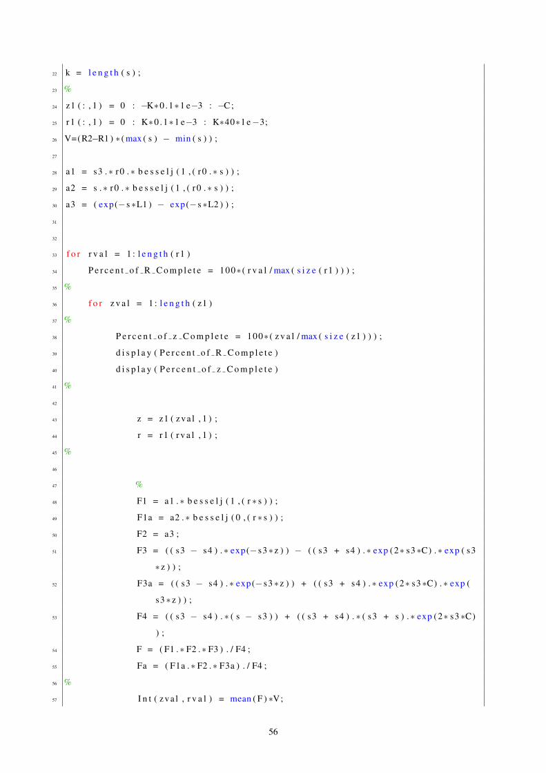
22 k = l e n g t h ( s ) ;
23 %
24 z1 ( : , 1 ) = 0 : −K∗0 .1∗1 e−3 : −C ;
25 r1 ( : , 1 ) = 0 : K∗0 .1∗1 e−3 : K∗40∗1 e−3;
26 V=(R2−R1 ) ∗ ( max ( s ) − min ( s ) ) ;
27
28 a1 = s3 .∗ r0 .∗ b e s s e l j ( 1 , ( r0 . ∗ s ) ) ;
29 a2 = s .∗ r0 .∗ b e s s e l j ( 1 , ( r0 . ∗ s ) ) ;
30 a3 = ( exp(− s ∗L1 ) − exp(− s ∗L2 ) ) ;
31
32
33 f o r r v a l = 1 : l e n g t h ( r1 )
34 P e r c e n t o f R C o m p l e t e = 100∗ ( r v a l / max ( s i z e ( r1 ) ) ) ;
35 %
36 f o r z v a l = 1 : l e n g t h ( z1 )
37 %
38 P e r c e n t o f z C o m p l e t e = 100∗ ( z v a l / max ( s i z e ( z1 ) ) ) ;
39 d i s p l a y ( P e r c e n t o f R C o m p l e t e )
40 d i s p l a y ( P e r c e n t o f z C o m p l e t e )
41 %
42
43 z = z1 ( zva l , 1 ) ;
44 r = r1 ( r v a l , 1 ) ;
45 %
46
47 %
48 F1 = a1 . ∗ b e s s e l j ( 1 , ( r ∗ s ) ) ;
49 F1a = a2 . ∗ b e s s e l j ( 0 , ( r ∗ s ) ) ;
50 F2 = a3 ;
51 F3 = ( ( s3 − s4 ) . ∗ exp(− s3 ∗z ) ) − ( ( s3 + s4 ) . ∗ exp (2∗ s3 ∗C) .∗ exp ( s3
∗z ) ) ;
52 F3a = ( ( s3 − s4 ) . ∗ exp(− s3 ∗z ) ) + ( ( s3 + s4 ) . ∗ exp (2∗ s3 ∗C) .∗ exp (
s3 ∗z ) ) ;
53 F4 = ( ( s3 − s4 ) . ∗ ( s − s3 ) ) + ( ( s3 + s4 ) . ∗ ( s3 + s ) . ∗ exp (2∗ s3 ∗C)
) ;
54 F = ( F1 . ∗ F2 .∗ F3 ) . / F4 ;
55 Fa = ( F1a . ∗ F2 .∗ F3a ) . / F4 ;
56 %
57 I n t ( zva l , r v a l ) = mean ( F ) ∗V;
56
58 I n t a ( zva l , r v a l ) = mean ( Fa ) ∗V;
59 %
60 F ( 1 : k , 1 ) = 0 ;
61 Fa ( 1 : k , 1 ) = 0 ;
62 F1 ( 1 : k , 1 ) = 0 ;
63 F1a ( 1 : k , 1 ) = 0 ;
64 F2 ( 1 : k , 1 ) = 0 ;
65 F3 ( 1 : k , 1 ) = 0 ;
66 F3a ( 1 : k , 1 ) = 0 ;
67 F4 ( 1 : k , 1 ) = 0 ;
68 %
69 c l c ;
70 %
71 end
72 %
73 c l c ;
74 %
75 end
76
77 c o n s t = Mu0∗N∗ I / ( ( L2−L1 ) ∗ ( R2−R1 ) ) ;
78 Br = I n t ∗ c o n s t ;
79 Bz = I n t a ∗ c o n s t ;
57
Appendix B
Dilation of parameters
In this chapter, we analytically prove that upon dilation of parameters the magnetic flux density remains an invari-
ant by individually analysing the dilated parameters.
Let us consider the original equations of the dilated variables
B′r = µ0i′0
∫∞
0s′3
(∫ r′2
r′1r′0J1(r′0s′)dr′0
)J1(r′s′)
[(e−s′L′1 − e−sL′2)
{. . .
.(s′3− s′4)e
−s′3z′ − (s′3 + s′4)e2s′3C′es′3z′
(s′3− s′4)(s′− s′3)+(s′3 + s′4)(s
′+ s′3)e2s′3C′
}]ds′
B′z =1r′
µ0i′0
∫∞
0
(∫ r′2
r′1r′0J1(r′0s′)dr′0
)(r′s′J0(r′s′)
)[(e−s′L′1 − e−s′L′2)
{. . .
.(s′3 + s′4)e
2s′3C′es′3z′ +(s′3− s′4)e−s′3z′
(s′3− s′4)(s′− s′3)+(s′3 + s′4)(s
′+ s′3)e2s′3C′
}]ds′
Applying the Dilation parameters discussed in the Section 6.4, we have
i′0 =N′I
(L′2−L′1)(R′2−R′1)
=kNI
k2(L2−L1)(R2−R1)
=NI
k(L2−L1)(R2−R1)
=i0k
(B.1)
∫ r2′
r1′r′0J1(r′0s′)dr′0 =
∫ r2
r1kr0J1(kr0
sk)dr0
= k∫ r2
r1r0J1(r0s)dr0 (B.2)
58
r′s′J0(r′s′) = krsk
J0(krsk)
= rsJ0(rs) (B.3)
e−s′L′1 − e−s′L′2 = e−sk kL1 − e−
sk kL2
= e−sL1 − e−sL2 (B.4)
(s′3− s′4)e−s′3z′ − (s′3 + s′4)e
2s′3C′es′3z′
(s′3− s′4)(s′− s′3)+(s′3 + s′4)(s
′+ s′3)e2s′3C′
=( s3
k −s4k )e−s3z− ( s3
k + s4k )e
2s3Ces3z
( s3k −
s4k )(
sk −
s3k )+( s3
k + s4k )(
sk +
s3k )e
2s′3C′
=1k1k2
(s3− s4)e−s3z− (s3 + s4)e2s3Ces3z
(s3− s4)(s− s3)+(s3 + s4)(s+ s3)e2s3C
= k(s3− s4)e−s3z− (s3 + s4)e2s3Ces3z
(s3− s4)(s− s3)+(s3 + s4)(s+ s3)e2s3C (B.5)
(s′3− s′4)e−s′3z′ +(s′3 + s′4)e
2s′3C′es′3z′
(s′3− s′4)(s′− s′3)+(s′3 + s′4)(s
′+ s′3)e2s′3C′
=( s3
k −s4k )e−s3z− ( s3
k + s4k )e
2s3Ces3z
( s3k −
s4k )(
sk −
s3k )+( s3
k + s4k )(
sk +
s3k )e
2s′3C′
=1k1k2
(s3− s4)e−s3z +(s3 + s4)e2s3Ces3z
(s3− s4)(s− s3)+(s3 + s4)(s+ s3)e2s3C
= k(s3− s4)e−s3z +(s3 + s4)e2s3Ces3z
(s3− s4)(s− s3)+(s3 + s4)(s+ s3)e2s3C (B.6)
Now having all the dilated variables, let us substitute them back in the original equation.
B′r = µ0i0∫
∞
0s′3
(∫ r′2
r′1r′0J1(r′0s′)dr′0
)J1(r′s′)
[(e−s′L′1 − e−sL′2)
{(s′3− s′4)e
−s′3z′ − (s′3 + s′4)e2s′3C′es′3z′
(s′3− s′4)(s′− s′3)+(s′3 + s′4)(s
′+ s′3)e2s′3C′
}]ds′
= µ0i0k
∫∞
0
s3
k
(k∫ r2
r1
r0J1(r0s)dr0
)J1(rs)
[(e−sL1 − e−sL2)
{k
(s3− s4)e−s3z− (s3 + s4)e2s3Ces3z
(s3− s4)(s− s3)+(s3 + s4)(s+ s3)e2s3C
}]ds
= µ0i0∫
∞
0s3
(∫ r2
r1
r0J1(r0s)dr0
)J1(rs)
[(e−sL1 − e−sL2)
{(s3− s4)e−s3z− (s3 + s4)e2s3Ces3z
(s3− s4)(s− s3)+(s3 + s4)(s+ s3)e2s3C
}]ds
(B.7)
= Br
B′z =1r′
µ0i′0
∫∞
0
(∫ r′2
r′1r′0J1(r′0s′)dr′0
)(r′s′J0(r′s′)
)[(e−s′L′1 − e−s′L′2)
{(s′3 + s′4)e
2s′3C′es′3z′ +(s′3− s′4)e−s′3z′
(s′3− s′4)(s′− s′3)+(s′3 + s′4)(s
′+ s′3)e2s′3C′
}]ds′
=1kr
µ0i0k
∫∞
0
(k∫ r2
r1
r0J1(r0s)dr0
)(rsJ0(rs)
)[(e−sL1 − e−sL2)
{k
(s3 + s4)e2s3Ces3z +(s3− s4)e−s3z
(s3− s4)(s− s3)+(s3 + s4)(s+ s3)e2s3C
}]ds
=1r
µ0i0∫
∞
0
(∫ r2
r1
r0J1(r0s)dr0
)(rsJ0(rs)
)[(e−sL1 − e−sL2)
{(s3 + s4)e2s3Ces3z +(s3− s4)e−s3z
(s3− s4)(s− s3)+(s3 + s4)(s+ s3)e2s3C
}]ds
(B.8)
= Bz
59

60
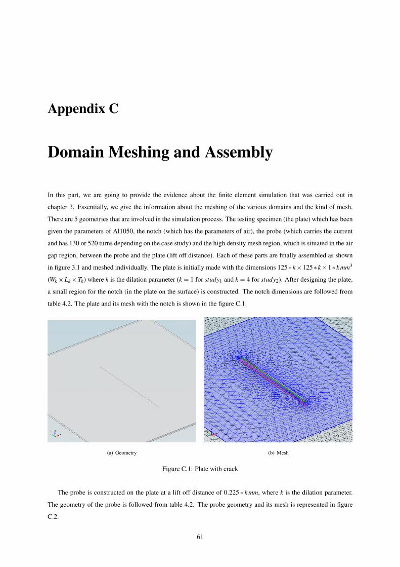
Appendix C
Domain Meshing and Assembly
In this part, we are going to provide the evidence about the finite element simulation that was carried out in
chapter 3. Essentially, we give the information about the meshing of the various domains and the kind of mesh.
There are 5 geometries that are involved in the simulation process. The testing specimen (the plate) which has been
given the parameters of Al1050, the notch (which has the parameters of air), the probe (which carries the current
and has 130 or 520 turns depending on the case study) and the high density mesh region, which is situated in the air
gap region, between the probe and the plate (lift off distance). Each of these parts are finally assembled as shown
in figure 3.1 and meshed individually. The plate is initially made with the dimensions 125∗k×125∗k×1∗k mm3
(Wk×Lk×Tk) where k is the dilation parameter (k = 1 for study1 and k = 4 for study2). After designing the plate,
a small region for the notch (in the plate on the surface) is constructed. The notch dimensions are followed from
table 4.2. The plate and its mesh with the notch is shown in the figure C.1.
(a) Geometry (b) Mesh
Figure C.1: Plate with crack
The probe is constructed on the plate at a lift off distance of 0.225 ∗ k mm, where k is the dilation parameter.
The geometry of the probe is followed from table 4.2. The probe geometry and its mesh is represented in figure
C.2.
61
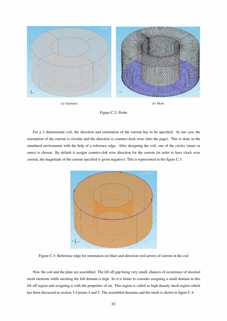
(a) Geometry (b) Mesh
Figure C.2: Probe
For a 3 dimensional coil, the direction and orientation of the current has to be specified. In our case the
orientation of the current is circular and the direction is counter-clock wise (into the page). This is done in the
simulated environment with the help of a reference edge. After designing the coil, one of the circles (inner or
outer) is chosen. By default it assigns counter-clok wise direction for the current (in order to have clock wise
current, the magnitude of the current specified is given negative). This is represented in the figure C.3.
Figure C.3: Reference edge for orientation (in blue) and direction (red arrow) of current in the coil
Now the coil and the plate are assembled. The lift off gap being very small, chances of occurrence of inverted
mesh elements while meshing the full domain is high. So it is better to consider assigning a small domain in this
lift off region and assigning it with the properties of air. This region is called as high density mesh region which
has been discussed in section 3.4 points 4 and 5. The assembled domains and the mesh is shown in figure C.4
62
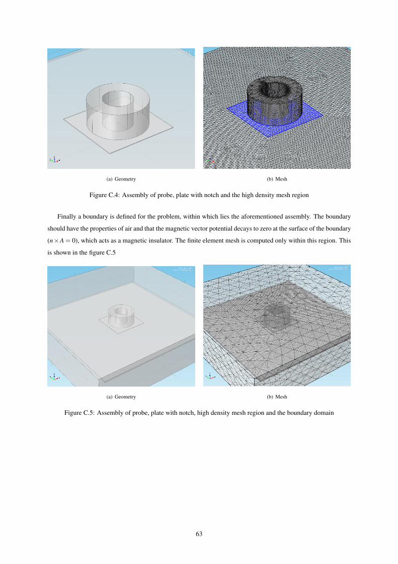
(a) Geometry (b) Mesh
Figure C.4: Assembly of probe, plate with notch and the high density mesh region
Finally a boundary is defined for the problem, within which lies the aforementioned assembly. The boundary
should have the properties of air and that the magnetic vector potential decays to zero at the surface of the boundary
(n×A = 0), which acts as a magnetic insulator. The finite element mesh is computed only within this region. This
is shown in the figure C.5
(a) Geometry (b) Mesh
Figure C.5: Assembly of probe, plate with notch, high density mesh region and the boundary domain
63

64