application of disjunctive cokriging to compare fertilizer ... · application of disjunctive...

Geoderma, 62 (1994) 247-263 247 Elsevier Science B.V., Amsterdam

Application of disjunctive cokriging to compare fertilizer scenarios on a field scale

P.A. Finke a and A. Stein b a Winand Staring Centre for Integrated Land, Soil and Water Research, P.O. Box 125,

6700 AC Wageningen, The Netherlands bDepartment of Soil Science and Geology, Agricultural University, P.O. Box 37,

6700 AA Wageningen, The Netherlands

(Received July 30, 1992; accepted after revision April 13, 1993)

ABSTRACT

To evaluate the effect of various levels of fertilizer applications, six fertilizing scenarios were analyzed by computer simulations using a process-based simulation model. By using simulation results of one of the fertilizer scenarios as a covariable in disjunctive cokriging (DCK), the number of simulations in the remaining scenarios could be reduced to 20% of the original number, while the prediction quality in fifty test points still satisfied two criteria based on the sample variance. When the conditional probability of exceeding a threshold value is to be mapped, an expanded data set is of limited use because some variance is lost in the expansion process.

INTRODUCTION

Agricultural practices are aiming at maximizing production by satisfying prerequisites for optimal plant growth and minimal stress. Examples of such practices are fertilizing and application of biocides. Unfortunately, some of these applications are reported to cause environmental problems due to leaching (Anderson et al., 1985; Commission of the European Communities, 1991 ). Leaching of fertilizer can occur when plants are not efficiently taking up the nutrients or when the demand is smaller than the nutrient status plus the application. Also soil physical properties strongly influence the occur- rence and magnitude of leaching. Leaching may show a strong spatial variation when nutrient status or soil physical properties are variable (Dagan and Bresler, 1983 ).

Minimization of leaching and maximization of production are possibly conflicting goals, because a uniform fertilizer application level that will max- imize production on the location with the worst nutrient status, may cause leaching on locations with a better nutrient status. A possible alternative is location-specific or soil-specific fertilizing instead of the usual field-specific fertilizing (Robert, 1988 ).

0016-7061/94/$07.00 © 1994 Elsevier Science B.V. All rights reserved. SSD10016-7061 (93) E0077-9

248 P.A. FINKE AND A. STEIN

In this study, the spatially varying impact of different scenarios of fertilizer applications is estimated by simulating water and solute transport on a large number of discrete points in an agricultural field. Throughout the text the word simulation is used to indicate the application of a process-based computer model which calculates the movement of water and nutrients in the unsaturated zone.

In this study, the nitrate leaching concentration was used to compare the effects of fertilizing scenarios. The leaching concentration is here defined as the annual net downward nitrate flux (rag/ha) at 80 cm depth expressed as a concentration in the annual net downward water flux (dm3/ha) at 80 cm depth. When scenarios are to be compared, results are usually interpreted by comparing an estimate of the spatial mean to some threshold value (Com- mission of the European Communities, 1991 ). In this study, the field average leaching concentration would have to be compared to the current threshold value of 50 mg nitrate/dm 3 or the pursued threshold value of 25 mg nitrate/ dm 3. A value of 49 mg/dm 3 would be acceptable whereas a value of 51 mg/ dm 3 would not. This is not realistic, because uncertainties caused by model inaccuracies and spatial variation of the property obscure the sensible use of absolute values. Hence, in this study a leaching criterion was formulated as: "Nowhere in the field the probability may be greater than 5% that a leaching concentration of 25 nag ni trate/dm a is exceeded". One may notice that this criterion is based on a probabilistic approach.

When scenario results are expressed as probabilities of exceeding a threshold value it allows the use of spatial variation of the property for decision making. However, it requires intensive sampling and the calculation of a large number of simulations to take the spatial variation into account. The use of existing spatial information, for instance soil characteristics sampled previously, may help to reduce the simulation effort.

The purpose of this study is to compare disjunctive kriging (DK) and disjunctive cokriging (DCK) (Matheron, 1976; Yates, 1986; Yates et al., 1986; Myers, 1988; Webster and Oliver, 1989) with respect to prediction quality and estimation of probabilities of exceedance. The main motive to make a comparison between DK and DCK was the high cost associated with simulation of nitrate leaching at many locations. To minimize the number of simulations, data from a previous simulation served as a covariable in DCK.

SIMULATION MODEL AND FERTILIZING SCENARIOS

Fertilizing scenarios were compared by simulation of the impact of each scenario on nitrate leaching and crop production in 402 soil profiles that were described in a field soil survey. To allow a realistic simulation of the spatially varying impact of a fertilizing scenario, model input variables showing spatial variation were determined at each profile or profile layer. Location-specific

APPLICATION OF DISJUNCTIVE COKRIGING 249

soil physical characteristics (bulk density and the water retention and hy- draulic conductivity functions) were generated for each location and depth using the available soil profile descriptions. The procedure followed is described in detail by Finke and Bosma (1993). Additionally, the texture and organic matter content were input to the model.

The model L E A C H N (Wagenet and Hutson, 1989; Hutson and Wagenet, 1991 ) was used for the simulation of water flow and nitrogen fate. In order to simulate crop production, the L E A C H N model was extended with a crop growth submodel. Model validation results (Finke, 1993) seem to support the working hypothesis that in the studied field spatial variability of model output exceeds model inaccuracy.

The fertilizing scenarios that were analyzed related to the current method to obtain the fertilizer application rate in the Netherlands. The advised fertilizer application rate is determined by:

Nadv = Nopt - aNmin ( 1 )

where Nad v is the advised nitrogen application (kg N/ha); and Nopt is the crop-specific optimum (kg N/ha) as determined in national trials (Nopt= 320 for potatoes and 115 for spring barley); a is a crop specific factor ( a - 1.1 for potatoes and 1 for spring barley) and Nm~ is the amount of inorganic nitrogen present in the rootable layer (kg N/ha). To investigate the impact of modi- fications of fertilizer additions on crop production and nitrate leaching, six different scenarios were defined in terms of the way the actual fertilizer application rate is calculated from the advised fertilizer application rate (Table 1 ). Simulations started with two years of fertilizing according to eq. ( 1 ) (scenario S-0), with initial nitrogen amounts corresponding to the level measured in the field. Thereafter, scenarios S-I to S-6 were simulated, each with an initial amount of nitrogen on each location that would be present after two

TABLE 1

Description of fertilizer scenarios. Nta. and Nopt are current advice and optimal levels in kg N/ha, Nmt. is the amount of available inorganic N in kg N/ha

Scenario Simulation N-application Nitrate leaching Leaching period rate concentration period depth (year/month) (kg N/ha) (year/month) (cm)

S-O 1987/4- 1989/4 N~v" 1987/4- 1988/4 80 S-I 1989/4- 1990/9 0.25N~v" 1989/4- 1990/4 80 S-2 1989/4- 1990/9 0.50N~v" 1989/4 - 1990/4 80 S-3 1989/4- 1990/9 N~v" 1989/4- 1990/4 80 S-4 1989/4 - 1990/9 1.50N~." 1989/4 - 1990/4 80 S-5 1989/4- 1990/9 2.00N~" 1989/4- 1990/4 80 S-6 1989/4 - 1990/9 2.00Nom-aN=i. 1989/4 - 1990/4 80

"Seeeq. (1).


years of fertilization according to S-0. This was done to avoid lagged nitrate leaching in the low input scenarios S-1 and S-2 due to high fertilizer application rates in the nearby past, that built up a pool of potentially leachable nitrogen. Scenarios S-0 and S-3 are thus equal in the way the fertilizer advice is calculated, but are different when the initial amounts of nitrogen (Nmin) are compared.

In scenarios S-4 and S-5 the actual fertilizer application would be 50% and 100% more than the advice. Scenario S-6 comprises an increase by 100% of the pursued level of inorganic nitrogen ( N o p t ) . This scenario is most likely to cause over-fertilization, because the amount of inorganic nitrogen in the soil is kept systematically much higher than the crops theoretically need. Scena- rios S-4 and S-5 also give more nitrogen than needed, but these scenarios are self-corrective: When the advice Nad,~ is small because Nr~in levels are near Nopt, which will happen when high fertilizer application were given in the past, also the modification will be small.

Scenario S-1 to S-6 comprised a simulation period of 17 months, from April 1, 1989 to September 1, 1990. In this period three crops were grown: spring barley, a catchcrop (ryegrass) and potatoes. The variable of interest in this study was the simulated nitrate concentration in the leaching water at 80 cm depth during the hydrological year from April 1, 1989 to April 1, 1990 for scenarios S-1 to S-6. For scenario S-0 the same variable was investigated, but over a different period: April 1, 1987 to April 1, 1988. Since the processes simulated in scenarios S-0 to S-6 are the same, and vary only in magnitude, it was expected that simulation outcomes of different scenarios would be highly correlated.

SPATIAL STATISTICS

Disjunctive kriging and disjunctive cokriging

One purpose of this study is to obtain field scale maps of the probability that nitrate loadings into the groundwater exceed a threshold value of 25 mg nitrate/din 3. The spatial prediction procedure disjunctive kriging (DK) aims at obtaining an estimator of this (conditional) probability at an unvisited location, taking its distribution into account. This requires the distribution of this variable to be known or to be estimated from available data. Because nitrate loadings are concentrations, a skewed distribution can occur, since negative concentrations do not exist. Also, distributions may be not uni- modal, because different soil types may show a different sensitivity to nitrogen leaching. This may require a transformation of the observed distribution into the standard normal distribution before probabilities at unvisited locations can be calculated. When disjunctive cokriging (DCK) is applied, observations on a covariable are used as well (Yates, 1986). In DK and DCK the


probability is conditioned on both the spatial distribution of the variable (s) and on a set of n observations, and hence is a conditional probability. It is assumed that the observations arc obtained from second order stationary random fields. For such fields, it is well-known that there always exists a function that transforms any observed distribution into the normal distribution (Kim et al., 1977).

Let n observations z(x~i), i= 1,...,n, from the field Z(x) be available on the predictand and m observations V(XEj), j= 1 ,...,m on a covariable. Let Pio,~ be the autocorrelation between the prediction location x0 and the ith observation location of the a th variable ( a = 1,2 ), and Pu.~p the crosscorrelation between the ith and the jth observation locations of variables a and fl (a,fl= 1,2 ). The autocorrelation and crosscorrelation can be estimated from the fitted variogram models by (Journel and Huijbrcgts, 1978 ):

P~'o,~ = 1 - 7i0,~ Pu.~, = 1 - 7~J,~___kp (2) 7o~,~ 7oo,~p

respectivily, where 7io,a is the semivariance at the distance between the prediction location Xo and the observation location i of variable a , 7,-j,~p is the crossvariance at the distance between locations i a n d j of the variables a and fl, 7oo,~ is the sill value ofthc variogram of variable a , and 7~o,~p is the sill value of the crossvariogram of the variables a and ft. The autocorrelogram is obtained from the variogram under the assumption of second order stationarity. The crosscorrelogram is obtained from the crossvariogram under the addi- tional assumption, that C~j,~p~ C~j,~, where C#,~p is the crosscovariance between an observation on a at location i and an observation on fl at locationj. An alternative approach would be to determine 2 crosscovariograms from the data and transform them into 2 crosscorrelograms.

In DK and in DCK 5 steps are distinguished to obtain both a prediction and the conditional probability of exceeding a cutoff value in an unvisited location Xo.

( 1 ) For the two variables, the observations arc transformed into standard- normal distributed values. This is usually achieved for each variable by put- ting the observations in ascending order, followed by setting the cumulative probability Q[Z(x~i) <~x] equal to ( i -0 .5 ) /n , where i is the number of observations less than or equal to x. By inverting the cumulative standard nor- real distribution for values thus obtained, transformed observations y(x~,) equivalent to z(x~) are found, which follow the standard normal distribution. Similarly for the second variable, observations u (x2j) equivalent to v(x2j) are found, also following the standard normal distribution. The coefficients of the Gaussian transform function and its inverse are determined in step 2:

(2) Based on the observed distributions of the observations on the two variables, assumed to be valid throughout the study area, the sequences of

2 5 2 P.A. FINKE AND A. STEIN

Hermite polynomials Y~ CkHk [ Y] and Y. DkHk[U] with coefficients Ck and D k ( see Appendix), are determined for the predictand and the covariable, respectively, upto a degree K that with sufficient precision represent the observed distributions. Values of Hermite polynomials Hk[y(xli)] and Hk [ U (XEj) ] are determined in the observation locations.

(3) In order to carry out a DK-prediction at an unvisited location Xo, K predictors at this location, each associated with one Hermite polynomial, are determined by weighing the values of the Hermite polynomial at the n observation points:

n

H'~ [ Y(xo ) ] = ~, bgkHk [ Y(xg) ] ( 3 ) / = 1

The weights bgk are determined by solving the linear disjunctive kriging system:

Pk =Rkbk (4)

in which Pk is a vector with elements Pgo, l raised to the power k, and Rk is a matrix with elements P;z~l raised to the power k. In the case of two variables, K predicted values, each associated with one Hermite polynomial, are determined by weighing the values of the Hermite polynomials at the n + m neigh- bouring observation points:

H~[ Y(xo) ] = ~,, bgkHk[ r(x , , ) ] + ~ ajkHk[ U(x2j) ] ( 5 ) i= 1 j= 1

The weights bgk and ajk are determined by solving the linear disjunctive cokriging system:

(P l , k~_ ( l~ l l , k R l 2 k ~ ( b k ~ 2.kJ--\RE,.k R221k]\ak/ (6)

in which Pa.k are vectors with elements p~. , , and the Ra#,k are matrices with elements # k V"

(4) The DK and the DCK predictors are obtained by adding the predictions of the K individual Hermite polynomials at Xo:

K

Z~K(Xo) = Y. CkH~[ Y(xo) ] (7) k = 0

using the coefficients Ck obtained previously. The prediction error variances for DK and DCK are then given by:

2 k~lk!C ~ a2K = E k!C2[ 1 --b'k.Okl aDCK= 1 -- (b'ga'k) ' (8) k = l

APPLICATION OF DISJUNCTIVE COKRIGING 2 5 3

respectively. Extension of these equations towards more than 1 covariable is straightforward.

(5) The conditional probability P that the predicted leaching concentration at location Xo exceeds a critical threshold (the cutoff value Yc) is estimated:

g Hk-l[YclH~[Y(xo)] P~,c(Xo) = 1 - ~(y~) +~(Y¢)k~ (9) =l k. I

where ¢( . ) is the standard normal density function and ~ ( - ) the standard normal distribution function (see Appendix).

Optimizing the number of simulations

The maximum number of possible simulation points was equal to 402. Simulations on all locations would result in a very high computing effort ( 11.2 CPU-days per scenario on a 486/25 MHz machine). We tried therefore to minimize the number of simulations and use the simulation results from scenario S-0 to complete the data set to n--402. Scenario S-0 results were expected to be highly correlated to scenario S-I to S-6 results, so disjunctive cokriging was used in the minimization procedure using scenario S-0 as a covariable.

A test set of 50 locations was selected at random without replacement from the available 402, so 352 locations were left for the predictand data set. Sce- nario S-0 was used to define two quality criteria. Interpolated values of nitrate leaching concentrations were obtained by disjunctive kriging to the 50 test points, and the mean variance of prediction error (MVPE) and the mean square error of prediction (MSEP) were calculated. Both the MVPE and the MSEP were expressed as a fraction of the sample variance at n=352, and these fractions were used as quality criteria for DCK. Relative instead of absolute criteria wcrc set, because leaching values and variance levels of scenarios S-I to S-6 were expected to bc different. An absolute criterion based on scenario S-0 could easily bc satisfied by a scenario with a lower mean leaching concentration or variance Icvel (the lower input scenarios), whereas it could bc impossible to satisfy by a scenario with higher mean or variance levels.

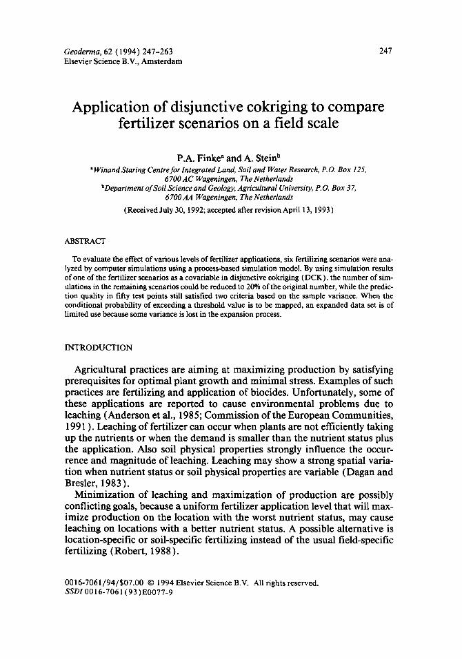
For scenarios S-I to S-6, a minimal data set was defined, consisting of 38 simulations, located on a triangular grid with a base distance of 48 m. to cover the entire field (Fig. I ). On the 50 test points simulations were done as well. Exponential and spherical variogram models were fitted to experimental sc- mivariances by a weighted least squares method. Crossvalidation, using or- dinary kriging, was done to choose the best performing model (McBratney and Webster, 1986). Disjunctive cokriging (DCK) predictions were carried out on the 50 test points, always using the nearest 12 observations on the predictand and 16 on the covariable, including I at thc tcstpoint. The MVPE

254 P . A . F I N K E A N D A . S T E I N

400

300

E

( 3 r--

200

100

+;

• 4 - . A - t - , , - + - A ,

z

. . . . . A . A t °, . A . . . . . A - X

÷A.+ . . I - . ~ ' + , ' ' + ' ' ~ ' \ 1 O0 200 300

distance (m)

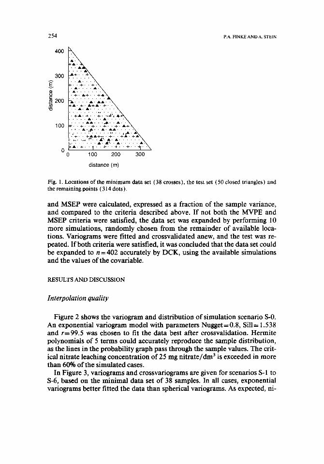
Fig. 1. Locations of the minimum data set (38 crosses), the test set (50 closed triangles) and the remaining points (314 dots).

and MSEP were calculated, expressed as a fraction of the sample variance, and compared to the criteria described above. If not both the MVPE and MSEP criteria were satisfied, the data set was expanded by performing 10 more simulations, randomly chosen from the remainder of available locations. Variograms were fitted and crossvalidated anew, and the test was re- peated. If both criteria were satisfied, it was concluded that the data set could be expanded to n = 402 accurately by DCK, using the available simulations and the values of the covariable.

RESULTS AND DISCUSSION

Interpolation quality

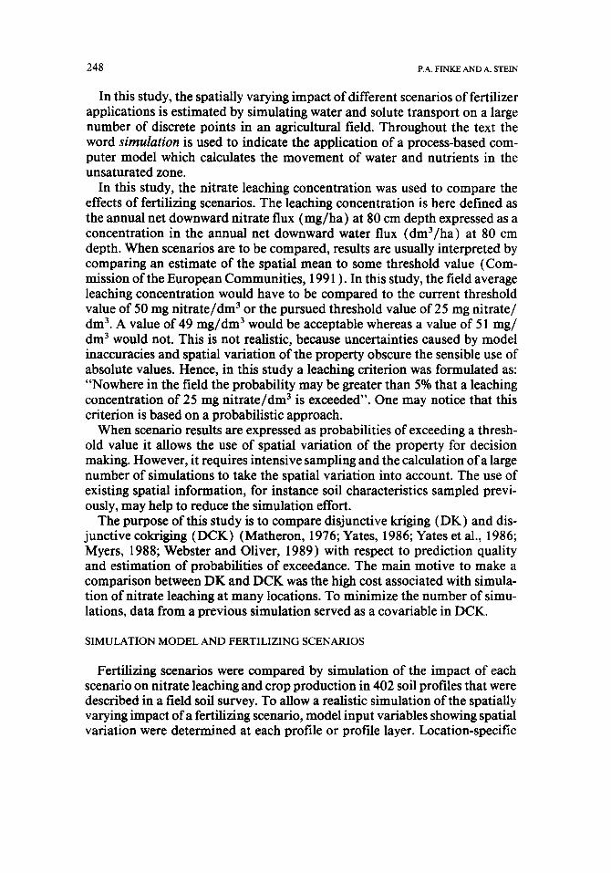
Figure 2 shows the variogram and distribution of simulation scenario S-0. An exponential variogram model with parameters Nugget=0.8, Sill= 1.538 and r=99.5 was chosen to fit the data best after crossvalidation. Hermite polynomials of 5 terms could accurately reproduce the sample distribution, as the lines in the probability graph pass through the sample values. The critical nitrate leaching concentration of 25 mg nitrate/din 3 is exceeded in more than 60% of the simulated cases.

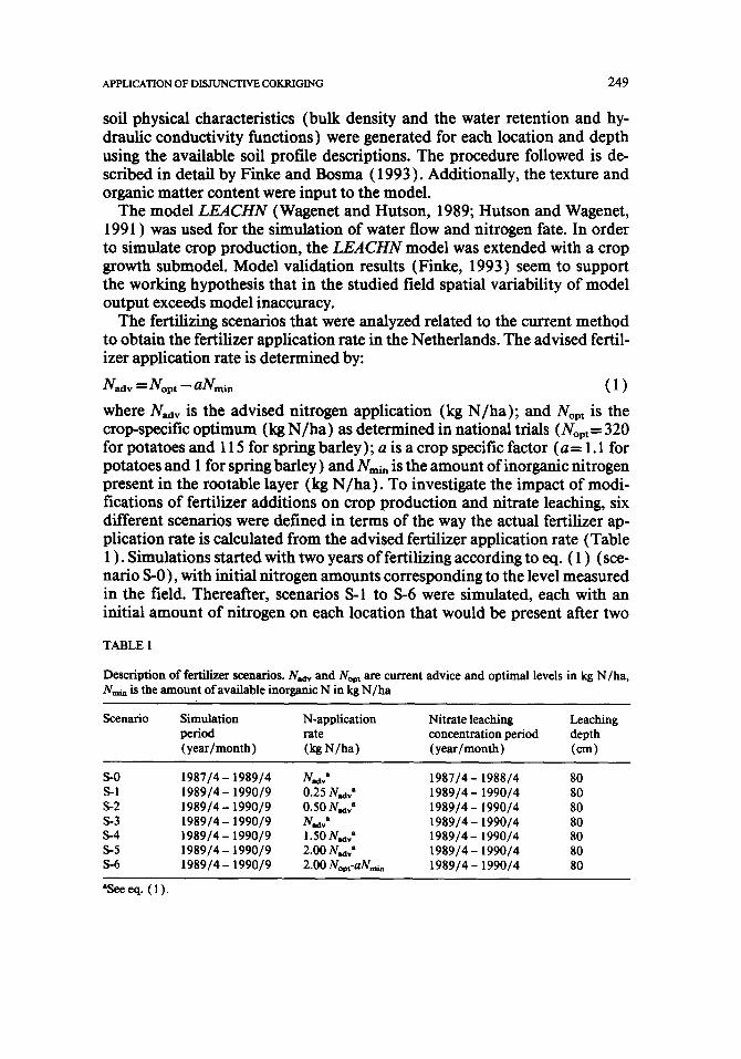
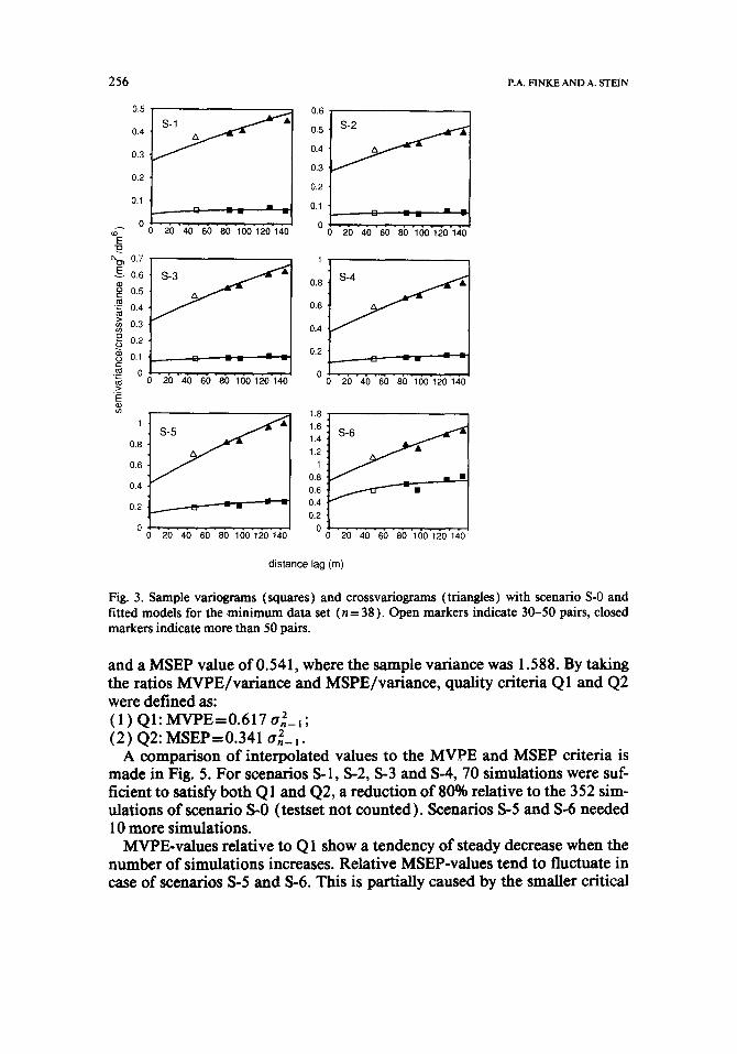
In Figure 3, variograms and crossvariograms are given for scenarios S-1 to S-6, based on the minimal data set of 38 samples. In all cases, exponential variograms better fitted the data than spherical variograms. As expected, ni-

APPLICATION OF DISJUNCTIVE COKRIGING 2 5 5

semivariance (mg 2/dm 6)

2

1.8

1.6

1.4

1.2

1

0.8

0.6

0.4

0.2

0 20 40

cumulative probability 1

0.9 b

0.8

0.7

0.6

0.5

0.4

0.3

0.2

0.1

0

, , ° i i , ° , ,

60 80 1 O0 1;tO 140 distance lag (m)

l b ' ' 3b ' Nitrate leaching concentration (mg/drn 3 )

Fig. 2. Sample and fitted model variograms (a) and sample and hermite transform distributions (b) of scenario S-0. Points indicate sample values, lines indicate model estimates.

trate leaching concentrations obtained with these scenarios were highly correlated to those obtained with scenario S-0 (Table 2 ).

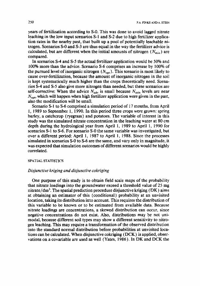
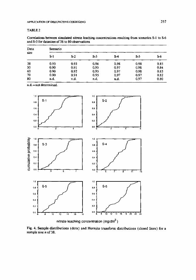
Sample distributions and reconstructed distributions based on 5-term Her- mite polynomials are given in Fig. 4. Sample distributions could be reconstructed well from normalized data by 5-term Hermite polynomials. The sample distributions of scenario S-3 (Fig. 4) and S-0 (Fig. 2) clearly differ. The higher leaching concentrations from S-0 indicate the lagged effect of a history of over-fertilization over the period before 1987. This effect is strongly reduced in the years that follow.

Interpolation of S-0 values to 50 test points yielded a MVPE value of 0.980


0.5

0.4

0.3

¢,o E lo

~:~ 0.7

0.6

o~ 0.5

>~ 0.4

0.3 O 0.2

O m 0.1

0

E

0.2

0.1

0 0

1

0.8

0.6

0.4

0.2

rl ~. ~ i -

20 40 60 80 100 120 14

20 40 60 80 100 120 140

20 40 60 80 100 120 140

0.6

0.5

0.4

0.3

0.2

0.1

0

i -- O .. ~_ i --,--~

0 20 40 60 80 100 120 140

1

0.8

0.6

0.4

0.2

0 . . . . . . . . . . . . . . 20 40 60 80 100 120 140

1.8 1.6 1.4 1.2

1 0.8 0.6 0.4 0.2

0 20 40 60 80 100 120 140

distance lag (m)

Fig. 3. Sample variograms (squares) and crossvariograms (triangles) with scenario S-0 and fitted models for the minimum data set (n = 38). Open markers indicate 30-50 pairs, closed markers indicate more than 50 pairs.

and a MSEP value of 0.541, where the sample variance was 1.588. By taking the ratios MVPE/variance and MSPE/variance, quality criteria Q1 and Q2 were defined as: ( 1 ) QI: M V P E = 0 . 6 1 7 a~_~; (2) Q2:MSEP=0.341 a~_~.

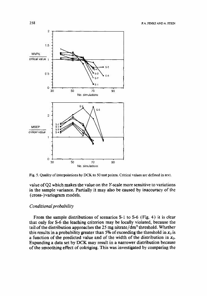
A comparison of interpolated values to the MVPE and MSEP criteria is made in Fig. 5. For scenarios S-1, S-2, S-3 and S-4, 70 simulations were sufficient to satisfy both Q1 and Q2, a reduction of 80% relative to the 352 simulations of scenario S-0 (testset not counted). Scenarios S-5 and S-6 needed 10 more simulations.

MVPE-values relative to Q 1 show a tendency of steady decrease when the number of simulations increases. Relative MSEP-values tend to fluctuate in case of scenarios S-5 and S-6. This is partially caused by the smaller critical


TABLE 2

Correlations between simulated nitrate leaching concentrations resulting from scenarios S-1 to S-6 and S-0 for datasizes of 38 to 80 observations

Data Scenario size

S-I S-2 S-3 S-4 S-5 S-6

38 0.93 0.93 0.96 0.98 0.98 0.85 50 0.90 0.91 0.95 0.97 0.98 0.84 60 0.90 0.92 0.95 0.97 0.98 0.83 70 0.90 0.91 0.95 0.97 0.97 0.82 80 n.d. n.d. n.d. n.d. 0.97 0.80

n.d. = not determined.

1.0

0.8

0.6

0.4

0.2

0.0

1.0

0.8

0.6

0,4

0,2

04)

s.2

/ .m

2 ~ L

E 0

1.0

0.8

0.6

0.4

0.2

0.0 3 5 7

1.0 ,

0.8

0.6 ¸

0.4 ¸

0 . 2 ,

0.0 3 5 7 9 11

1,0

0.8

0.6

0.4

0.2

0.0 6 18 8 10 12 14 16

1,0

0.8

0.6

0.4

0.2

0.0 8 10 12 14 16 18 20 22 24

nitrate leaching concentration (mg/dm 3 )

Fig. 4. Sample distributions (dots) and Hermitc transform distributions (closed lines) for a sample size n o f 38.


1.5

MVPE critical value 1

0.5

30 90

' ~ " ~ ~ s-5

S-6

sb 7b No. simulations

MSEP critical value

S-6

S-2 S-1 S-3 S-4

30 50 70 90 NO. simulations

Fig. 5. Quality of interpolations by DCK to 50 test points. Critical values are defined in text.

value of Q2 which makes the value on the Y-scale more sensitive to variations in the sample variance. Partially it may also be caused by inaccuracy of the (cross-) variogram models.

Conditional probability

From the sample distributions of scenarios S-1 to S-6 (Fig. 4) it is clear that only for S-6 the leaching criterion may be locally violated, because the tail of the distribution approaches the 25 mg nitrate/dm 3 threshold. Whether this results in a probability greater than 5% of exceeding the threshold in Xo is a function of the predicted value and of the width of the distribution in Xo. Expanding a data set by DCK may result in a narrower distribution because of the smoothing effect of cokriging. This was investigated by comparing the


cumulative probability

1

0.5

1

S

0 | 0 10 20 30

nitrate leaching concentration (mg/dm 3)

40

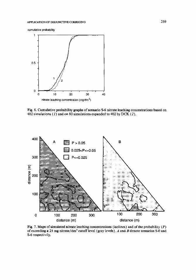
Fig. 6. Cumulative probability graphs of scenario S-6 nitrate leaching concentrations based on 402 simulations (1) and on 80 simulations expanded to 402 by DCK (2).

400

300

A

E v

=o 200

"o

100

0 1 O0 200 300 1 O0 200 300

distance (m) distance (m)

Fig. 7. Maps of simulated nitrate leaching concentrations (isolines) and of the probability (P) of exceeding a 25 mg ni t rate/dm 3 cutoff level (gray levels). A and B denote scenarios S-0 and S-6 respectivily.

260 P.A. FTNKE AND A. STEIN

distribution of a data set of n = 80, expanded by DCK to n = 402, to a data set obtained by actually performing the simulations of scenario S-6 on all 402 locations. In Fig. 6, the cumulative probability density graphs are given of scenario S-6, based on the complete data set (n = 402 ) and the smaller data set expanded using DCK to n = 402. The expanded data set evidently exhibits a narrower distribution, indicating that reduction of the number of simulations by DCK is not advisable when probabilities of exceedance are to be estimated.

A map of the conditional probability of exceeding the threshold leaching concentration of 25 mg nitrate/din 3 at fertilizer levels corresponding to scenarios S-0 and S-6 is given in Fig. 7. Scenario S-0 results in leaching concentrations clearly exceeding the criterion. The leaching criterion is scarcely exceeded in case of scenario S-6. In 1.4% of the field area the probability of exceeding the threshold level is higher than 5%, implicating the area where the scenario is rejected. A map of scenario S-6 (not shown ), whereby the data set was expanded to 402 simulations by DCK first, did not show any areas where the leaching criterion was exceeded, because of the associated loss of variance.

As a result, it was concluded that pursued nitrate leaching concentrations of 25 mg nitrate/dm 3 will be violated with high probability for one hydrological year after lowering fertilizer applications because of lagged leaching as a result of a history of over-fertilization (scenario S-0). In the first hydrological year, fertilizing according to scenario S-6 will lead to a locally too high probability that the pursued level is exceeded. All other scenarios are safe in terms of nitrate leaching on the short term. This implies that scenario S-5 would be the most attractive to implement, because it will give the highest crop yields.

CONCLUSIONS

( 1 ) Disjunctive cokriging with a highly correlated covariable greatly reduced the number of simulations in a scenario analysis without loss of prediction quality in terms of MSEP and MVPE.

(2) When the cutoff-value is in the tail of the distribution, it is important to estimate the distribution function correctly. It is then better to perform many simulations than to use a covariable to expand the data set, because variance is lost in this process.

ACKNOWLEDGEMENTS

This research was partly carried out during a stay of the second author at the University of Arizona, with a grant of the Netherlands Integrated Soil Research Programme. Financial support by EC-project EV4V*0098-NL "Ni- trate in Soils" is gratefully acknowledged.


APPENDIX. HERMITE POLYNOMIALS AND CONDITIONAL PROBABILITY

Hermite polynomials

Hermite polynomials Hk(y) of order k are defined as:

Hk(y) = ( -- 1 )ke~-Y~/2~ dk [e t-y2/2~ ] (A1) dy k

It is easily seen that Ho(y) = 1 and H~ (y) =y. A simple relation exists between Hk÷ ~ (y), Hk(y) and Hk_ 1 (Y) for k>~ 2: Hk÷ ~ (y) =YHk(Y) -kHk_ ~ (y). Hermite polynomials are orthogonal with respect to the weighting function exp ( - y 2 / 2 ) on the interval [ - oo,oo ], that is:

i Hi(y)Hj(y) e-y2/2dy - - 0 0

i ! x /~ ----t~ij (A2)

with $ij=0 when i~ j and $o= 1 when i=j. Many functions can be approximated by a finite series of Hermite

polynomials:

f ( x ) = ~ CkHk(X) (A3) k = O

where fitting the coefficients Ck is based upon the orthogonality relationship (A2). It may be done efficiently by means of Hermite integration (Abramow- itz and Stegun, 1965 ).

Conditional probability

An estimator of the conditional probability that a variable at a location Xo exceeds a cutoff level z¢ is based on the indicator function Oyo (Y) = 1 if Y>~ y¢ and Oyc (Y) -- 0 if Y<y~, where Yc is the transformed cutofflevel related to the actual cutoff level z~ and Y is the transformed variable related to Z. The conditional expectation of ~gyo in the unvisited location Xo is given by:

E [0yci Y(xo) )1Y(x,) ] = P [0yo(Y(xo) ) = 11Y(x,) ] (A4)

since Oyo is either 1 or 0. The conditional probability of Z(xo) exceeding z¢ is thus estimated by the conditional expectation of the indicator function Oro (Y) in location Xo. Now, Oyo(Y(xo)) can be estimated when it is expanded in Hermite polynomials (Yates et al., 1986) as:

K

Or~(Y(xo) )= ~ Oknk(Y(Xo) ) (A5) k = 0


where the Hermite coefficients Ok for order k are determined using the orthogonality relations (A2): do = 1 - ~(Yc), and Oh= ~ (Yc)H~_ 1 (Yc)/k!, where • (. ) is the cumulative standard normal probability distribution and ¢ (") its probability density function.

Combination of (A4) with the DK or the DCK predictor gives the conditional probability that Y(xo) ~< yc, estimated by the sum of the predictions of the Hermite polynomials that describe Oy c (Y(xo) ):

K

P*(xo) = 1 -- ~(Yc) +~(Yc) ~, Hk-1 (y~)H~(Y(xo) )/k! (A6) k = l

REFERENCES

Abramowitz, M. and Stegun, A., 1965. Handbook of Mathematical Functions. Dover, New York. Anderson, G.D., Opaluch, J.J. and Sullivan, W.M., 1985. Nonpoint agricultural pollution: pes-

ticide contamination of groundwater supplies. Am. J. Agric. Econom., 67 ( 5 ): 1238-1243. Commission of the European Communities, 1991. Soil and groundwater research rep. II. Ni-

trate in Soils. CEC, Luxembourg. Dagan, G. and Bresler, E., 1983. Unsaturated flow in spatially variable fields. 1. Derivation of

models of infiltration and redistribution. Water Resour. Res., 19:413-420. Finke, P.A., 1993. Field scale variability of soil structure and its impact on crop growth and

nitrate leaching in the analysis of fertilizing scenarios. In: R.J. Wagenet and J. Bouma (Edi- tors), Operational Methods to Characterize Soil Behaviour in Space and Time. Geoderma, 60: 89-107.

Finke, P.A. and Bosma, W.J.P., 1993. Obtaining basic simulation data for a heterogeneous field with stratified marine soils. Hydrol. Process., 7: 63-75.

Hutson, J.L. and Wagenet, R.J., 1991. Simulating nitrogen dynamics in soils using a determin- istic model. Soil Use Manage., 7 (2): 74-78.

Johnsson, H., Bergstrom, L., ansson, P.-E. and Paustian, Ka., 1987. Simulated nitrogen dynamics and losses in a layered agricultural soil. Agric. Ecosyst. Environ., 18: 333-356.

Journel, A.G. and Huijbregts, Ch.J., 1978. Mining Geostatistics. Academic Press, London. Kim, Y.C., Myers, D.E. and Knudsen, H.P., 1977. Advanced geostatistics in ore reserve esti-

mation and mine planning practioner's guide. Report to the U.S. Energy Research and De- velopment Administration, subcontract No. 76-003-E, Phase II.

Matheron, G., 1976. A simple substitute for conditional expectation: the disjunctive kriging. In: M. Guarascio et al. (Editors), Advanced Geostatistics in the Mining Industry. NATO Ad- vanced Study Institute Series. Reidel, Dordreeht, pp. 221-236.

McBratney, A.B. and Webster, R., 1986. Choosing functions for semivariograms and fitting them to sampling estimates. J. Soil Sci., 37:617-639.

Myers, D.E., 1988. Some aspects of multivariate analysis. In: C.F. Chung et al. (Editors), Quan- titative Analysis of Mineral and Energy Resources. Reidel, Dordrecht, pp. 669-687.

Robert, P.C., 1988. Land evaluation at farm level using soil survey information systems. In: J. Bouma and A.K. Bregt (Editors), Land Qualities in Space and time. Proc. Symp. orga- nized by the International Society of Soil Science (ISSS) Wageningen, The Netherlands, 22- 26 August 1988. Pudoc, Wageningen, pp. 299-311.

Wagenet, R.J. and Hutson, J.L., 1989. Leaching estimation and chemistry model: a process- based model of water and solute movement, transformations, plant uptake and chemical reactions in the unsaturated zone. Continuum Water Resources Institute, Cornell Univer- sity, NY.


Webster, R. and Oliver, M.A., 1989. Optimal interpolation and isarithmic mapping of soil properties. VI. Disjunctive Kriging and mapping the conditional probability. J. Soil Sci., 40: 497- 512.

Yates, S.R., 1986. Disjunctive Kriging 3. Disjunctive Cokriging. Water Resour. Res., 22(5): 1371-1376.

Yates, S.R., Warrick, A.W. and Myers, D.E., 1986. Disjunctive Kriging 1. Overview of estimation and conditional probability. Water Resour. Res., 22 (5): 615-621.

application of disjunctive cokriging to compare fertilizer ... · application of disjunctive...

Documents